OPEN-SOURCE SCRIPT
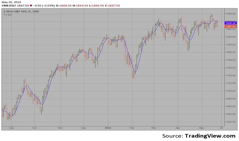
T3 Average
This indicator plots the moving average described in the January, 1998 issue
of S&C, p.57, "Smoothing Techniques for More Accurate Signals", by Tim Tillson.
This indicator plots T3 moving average presented in Figure 4 in the article.
T3 indicator is a moving average which is calculated according to formula:
T3(n) = GD(GD(GD(n))),
where GD - generalized DEMA (Double EMA) and calculating according to this:
GD(n,v) = EMA(n) * (1+v)-EMA(EMA(n)) * v,
where "v" is volume factor, which determines how hot the moving average’s response
to linear trends will be. The author advises to use v=0.7.
When v = 0, GD = EMA, and when v = 1, GD = DEMA. In between, GD is a less aggressive
version of DEMA. By using a value for v less than1, trader cure the multiple DEMA
overshoot problem but at the cost of accepting some additional phase delay.
In filter theory terminology, T3 is a six-pole nonlinear Kalman filter. Kalman
filters are ones that use the error — in this case, (time series - EMA(n)) —
to correct themselves. In the realm of technical analysis, these are called adaptive
moving averages; they track the time series more aggres-sively when it is making large
moves. Tim Tillson is a software project manager at Hewlett-Packard, with degrees in
mathematics and computer science. He has privately traded options and equities for 15 years.
Script open-source
Nello spirito di TradingView, l'autore di questo script lo ha reso open source, in modo che i trader possano esaminarne e verificarne la funzionalità. Complimenti all'autore! Sebbene sia possibile utilizzarlo gratuitamente, ricordiamo che la ripubblicazione del codice è soggetta al nostro Regolamento.
Declinazione di responsabilità
Le informazioni e le pubblicazioni non sono intese come, e non costituiscono, consulenza o raccomandazioni finanziarie, di investimento, di trading o di altro tipo fornite o approvate da TradingView. Per ulteriori informazioni, consultare i Termini di utilizzo.