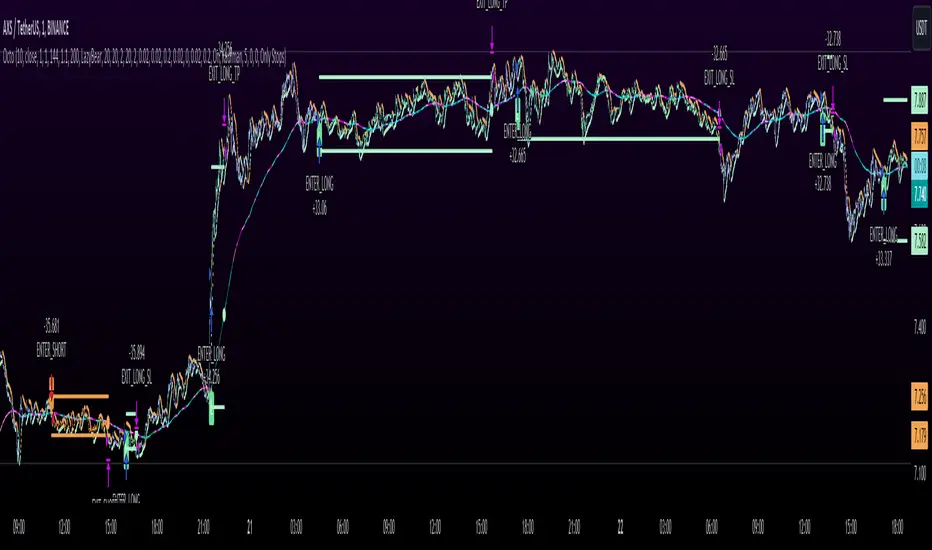
Octopus Nest Strategy Hello Fellas,
Hereby, I come up with a popular strategy from YouTube called Octopus Nest Strategy. It is a no repaint, lower timeframe scalping strategy utilizing PSAR, EMA and TTM Squeeze.
The strategy considers these market factors:
PSAR -> Trend
EMA -> Trend
TTM Squeeze -> Momentum and Volatility by incorporating Bollinger Bands and Keltner Channels
Note: As you can see there is a potential improvement by incorporating volume.
What's Different Compared To The Original Strategy?
I added an option which allows users to use the Adaptive PSAR of @loxx, which will hopefully improve results sometimes.
Signals
Enter Long -> source above EMA 100, source crosses above PSAR and TTM Squeeze crosses above 0
Enter Short -> source below EMA 100, source crosses below PSAR and TTM Squeeze crosses below 0
Exit Long and Exit Short are triggered from the risk management. Thus, it will just exit on SL or TP.
Risk Management
"High Low Stop Loss" and "Automatic High Low Take Profit" are used here.
High Low Stop Loss: Utilizes the last high for short and the last low for long to calculate the stop loss level. The last high or low gets multiplied by the user-defined multiplicator and if no recent high or low was found it uses the backup multiplier.
Automatic High Low Take Profit: Utilizes the current stop loss level of "High Low Stop Loss" and gets calculated by the user-defined risk ratio.
Now, follows the bunch of knowledge for the more inexperienced readers.
PSAR: Parabolic Stop And Reverse; Developed by J. Welles Wilders and a classic trend reversal indicator.
The indicator works most effectively in trending markets where large price moves allow traders to capture significant gains. When a security’s price is range-bound, the indicator will constantly be reversing, resulting in multiple low-profit or losing trades.
TTM Squeeze: TTM Squeeze is a volatility and momentum indicator introduced by John Carter of Trade the Markets (now Simpler Trading), which capitalizes on the tendency for price to break out strongly after consolidating in a tight trading range.
The volatility component of the TTM Squeeze indicator measures price compression using Bollinger Bands and Keltner Channels. If the Bollinger Bands are completely enclosed within the Keltner Channels, that indicates a period of very low volatility. This state is known as the squeeze. When the Bollinger Bands expand and move back outside of the Keltner Channel, the squeeze is said to have “fired”: volatility increases and prices are likely to break out of that tight trading range in one direction or the other. The on/off state of the squeeze is shown with small dots on the zero line of the indicator: red dots indicate the squeeze is on, and green dots indicate the squeeze is off.
EMA: Exponential Moving Average; Like a simple moving average, but with exponential weighting of the input data.
Don't forget to check out the settings and keep it up.
Best regards,
simwai
---
Credits to:
@loxx
@Bjorgum
@Greeny
Adaptive
Backtesting ModuleDo you often find yourself creating new 'strategy()' scripts for each trading system? Are you unable to focus on generating new systems due to fatigue and time loss incurred in the process? Here's a potential solution: the 'Backtesting Module' :)
INTRODUCTION
Every trading system is based on four basic conditions: long entry, long exit, short entry and short exit (which are typically defined as boolean series in Pine Script).
If you can define the conditions generated by your trading system as a series of integers, it becomes possible to use these variables in different scripts in efficient ways. (Pine Script is a convenient language that allows you to use the integer output of one indicator as a source in another.)
The 'Backtesting Module' is a dynamic strategy script designed to adapt to your signals. It boasts two notable features:
⮞ It produces a backtest report using the entry and exit variables you define.
⮞ It not only serves for system testing but also to combine independent signals into a single system. (This functionality enables to create complex strategies and report on their success!)
The module tests Golden and Death cross signals by default, when you enter your own conditions the default signals will be neutralized. The methodology is described below.
PREPARATION
There are three simple steps to connect your own indicator to the Module.
STEP 1
Firstly, you must define entry and exit variables in your own script. Let's elucidate it with a straightforward example. Consider a system generating long and short signals based on the intersections of two moving averages. Consequently, our conditions would be as follows:
// Signals
long = ta.crossover(ta.sma(close, 14), ta.sma(close, 28))
short = ta.crossunder(ta.sma(close, 14), ta.sma(close, 28))
Now, the question is: How can we convert boolean variables into integer variables? The answer is conditional ternary block, defined as follows:
// Entry & Exit
long_entry = long ? 1 : 0
long_exit = short ? 1 : 0
short_entry = short ? 1 : 0
short_exit = long ? 1 : 0
The mechanics of the Entry & Exit variables are simple. The variable takes on a value of 1 when your trading system generates the signal and if your system does not produce any signal, variable returns 0. In this example, you see how exit signals can be generated in a trading system that only contains entry signals. If you have a system with original exit signals, you can also use them directly. (Please mind the NOTES section below).
STEP 2
To utilize the Entry & Exit variables as source in another script, they must be plotted on the chart. Therefore, the final detail to include in the script containing your trading system would be as follows:
// Plot The Output
plot(long_entry, "Long Entry", display=display.data_window, editable=false)
plot(long_exit, "Long Exit", display=display.data_window, editable=false)
plot(short_entry, "Short Entry", display=display.data_window, editable=false)
plot(short_exit, "Short Exit", display=display.data_window, editable=false)
STEP 3
Now, we are ready to test the system! Load the Backtesting Module indicator onto the chart along with your trading system/indicator. Then set the outputs of your system (Long Entry, Long Exit, Short Entry, Short Exit) as source in the module. That's it.
FEATURES & ORIGINALITY
⮞ Primarily, this script has been created to provide you with an easy and practical method when testing your trading system.
⮞ I thought it might be nice to visualize a few useful results. The Backtesting Module provides insights into the outcomes of both long and short trades by computing the number of trades and the success percentage.
⮞ Through the 'Trade' parameter, users can specify the market direction in which the indicator is permitted to initiate positions.
⮞ Users have the flexibility to define the date range for the test.
⮞ There are optional features allowing users to plot entry prices on the chart and customize bar colors.
⮞ The report and the test date range are presented in a table on the chart screen. The entry price can be monitored in the data window.
⮞ Note that results are based on realized returns, and the open trade is not included in the displayed results. (The only exception is the 'Unrealized PNL' result in the table.)
STRATEGY SETTINGS
The default parameters are as follows:
⮞ Initial Balance : 10000 (in units of currency)
⮞ Quantity : 10% of equity
⮞ Commission : 0.04%
⮞ Slippage : 0
⮞ Dataset : All bars in the chart
For a realistic backtest result, you should size trades to only risk sustainable amounts of equity. Do not risk more than 5-10% on a trade. And ALWAYS configure your commission and slippage parameters according to pessimistic scenarios!
NOTES
⮞ This script is intended solely for development purposes. And it'll will be available for all the indicators I publish.
⮞ In this version of the module, all order types are designed as market orders. The exit size is the sum of the entry size.
⮞ As your trading conditions grow more intricate, you might need to define the outputs of your system in alternative ways. The method outlined in this description is tailored for straightforward signal structures.
⮞ Additionally, depending on the structure of your trading system, the backtest module may require further development. This encompasses stop-loss, take-profit, specific exit orders, quantity, margin and risk management calculations. I am considering releasing improvements that consider these options in future versions.
⮞ An example of how complex trading signals can be generated is the OTT Collection. If you're interested in seeing how the signals are constructed, you can use the link below.
THANKS
Special thanks to PineCoders for their valuable moderation efforts.
I hope this will be a useful example for the TradingView community...
DISCLAIMER
This is just an indicator, nothing more. It is provided for informational and educational purposes exclusively. The utilization of this script does not constitute professional or financial advice. The user solely bears the responsibility for risks associated with script usage. Do not forget to manage your risk. And trade as safely as possible. Best of luck!

Adaptive Price Channel StrategyThis strategy is an adaptive price channel strategy based on the Average True Range (ATR) indicator and the Average Directional Index (ADX). It aims to identify sideways markets and trends in the price movements and make trades accordingly.
The strategy uses a length parameter for the ATR and ADX indicators, which determines the length of the calculation for these indicators. The strategy also uses an ATR multiplier, which is multiplied by the ATR to determine the upper and lower bounds of the price channel.
The first step of the strategy is to calculate the highest high (HH) and lowest low (LL) over the specified length. The ATR is also calculated over the same length. Then the strategy calculates the positive directional indicator (+DI) and negative directional indicator (-DI) based on the up and down moves in the price, and uses these to calculate the ADX.
If the ADX is less than 25, the market is considered to be in a sideways phase. In this case, if the price closes above the upper bound of the price channel (HH - ATR multiplier * ATR), the strategy enters a long position, and if the price closes below the lower bound of the price channel (LL + ATR multiplier * ATR), the strategy enters a short position.
If the ADX is greater than or equal to 25 and the +DI is greater than the -DI, the market is considered to be in a bullish phase. In this case, if the price closes above the upper bound of the price channel, the strategy enters a long position. If the ADX is greater than or equal to 25 and the +DI is less than the -DI, the market is considered to be in a bearish phase. In this case, if the price closes below the lower bound of the price channel, the strategy enters a short position.
The strategy exits a position after a certain number of bars have passed since the entry, as specified by the exit_length input.
In summary, this strategy attempts to trade in accordance with the prevailing market conditions by identifying sideways markets and trends and making trades based on price movements within a dynamically-adjusted price channel.
This strategy takes a read on the market and either takes a channel strategy or trades volatility based on current trend. Works well on 2, 3 ,4, 12 hour for BTC. It’s my first attempt and creating a strategy. I am very interested in constructive criticism. I will look into better risk management, maybe a trailing stop loss. Other suggestions welcome. This is my first attempt at a strategy.
Here are the settings I used.
Inputs
Length 20
Exit 10
ATR 3.2
Dates I picked when I got into Crypto
Properties
Capital 1000
Order size 2 Contracts
Pyramiding 1
Commission .05

STD-Filterd, R-squared Adaptive T3 w/ Dynamic Zones BT [Loxx]STD-Filterd, R-squared Adaptive T3 w/ Dynamic Zones BT is the backtest strategy for "STD-Filterd, R-squared Adaptive T3 w/ Dynamic Zones " seen below:
Included:
This backtest uses a special implementation of ATR and ATR smoothing called "True Range Double" which is a range calculation that accounts for volatility skew.
You can set the backtest to 1-2 take profits with stop-loss
Signals can't exit on the same candle as the entry, this is coded in a way for 1-candle delay post entry
This should be coupled with the INDICATOR version linked above for the alerts and signals. Strategies won't paint the signal "L" or "S" until the entry actually happens, but indicators allow this, which is repainting on current candle, but this is an FYI if you want to get serious with Pinescript algorithmic botting
You can restrict the backtest by dates
It is advised that you understand what Heikin-Ashi candles do to strategies, the default settings for this backtest is NON Heikin-Ashi candles but you have the ability to change that in the source selection
This is a mathematically heavy, heavy-lifting strategy with multi-layered adaptivity. Make sure you do your own research so you understand what is happening here. This can be used as its own trading system without any other oscillators, moving average baselines, or volatility/momentum confirmation indicators.
What is the T3 moving average?
Better Moving Averages Tim Tillson
November 1, 1998
Tim Tillson is a software project manager at Hewlett-Packard, with degrees in Mathematics and Computer Science. He has privately traded options and equities for 15 years.
Introduction
"Digital filtering includes the process of smoothing, predicting, differentiating, integrating, separation of signals, and removal of noise from a signal. Thus many people who do such things are actually using digital filters without realizing that they are; being unacquainted with the theory, they neither understand what they have done nor the possibilities of what they might have done."
This quote from R. W. Hamming applies to the vast majority of indicators in technical analysis . Moving averages, be they simple, weighted, or exponential, are lowpass filters; low frequency components in the signal pass through with little attenuation, while high frequencies are severely reduced.
"Oscillator" type indicators (such as MACD , Momentum, Relative Strength Index ) are another type of digital filter called a differentiator.
Tushar Chande has observed that many popular oscillators are highly correlated, which is sensible because they are trying to measure the rate of change of the underlying time series, i.e., are trying to be the first and second derivatives we all learned about in Calculus.
We use moving averages (lowpass filters) in technical analysis to remove the random noise from a time series, to discern the underlying trend or to determine prices at which we will take action. A perfect moving average would have two attributes:
It would be smooth, not sensitive to random noise in the underlying time series. Another way of saying this is that its derivative would not spuriously alternate between positive and negative values.
It would not lag behind the time series it is computed from. Lag, of course, produces late buy or sell signals that kill profits.
The only way one can compute a perfect moving average is to have knowledge of the future, and if we had that, we would buy one lottery ticket a week rather than trade!
Having said this, we can still improve on the conventional simple, weighted, or exponential moving averages. Here's how:
Two Interesting Moving Averages
We will examine two benchmark moving averages based on Linear Regression analysis.
In both cases, a Linear Regression line of length n is fitted to price data.
I call the first moving average ILRS, which stands for Integral of Linear Regression Slope. One simply integrates the slope of a linear regression line as it is successively fitted in a moving window of length n across the data, with the constant of integration being a simple moving average of the first n points. Put another way, the derivative of ILRS is the linear regression slope. Note that ILRS is not the same as a SMA ( simple moving average ) of length n, which is actually the midpoint of the linear regression line as it moves across the data.
We can measure the lag of moving averages with respect to a linear trend by computing how they behave when the input is a line with unit slope. Both SMA (n) and ILRS(n) have lag of n/2, but ILRS is much smoother than SMA .
Our second benchmark moving average is well known, called EPMA or End Point Moving Average. It is the endpoint of the linear regression line of length n as it is fitted across the data. EPMA hugs the data more closely than a simple or exponential moving average of the same length. The price we pay for this is that it is much noisier (less smooth) than ILRS, and it also has the annoying property that it overshoots the data when linear trends are present.
However, EPMA has a lag of 0 with respect to linear input! This makes sense because a linear regression line will fit linear input perfectly, and the endpoint of the LR line will be on the input line.
These two moving averages frame the tradeoffs that we are facing. On one extreme we have ILRS, which is very smooth and has considerable phase lag. EPMA has 0 phase lag, but is too noisy and overshoots. We would like to construct a better moving average which is as smooth as ILRS, but runs closer to where EPMA lies, without the overshoot.
A easy way to attempt this is to split the difference, i.e. use (ILRS(n)+EPMA(n))/2. This will give us a moving average (call it IE /2) which runs in between the two, has phase lag of n/4 but still inherits considerable noise from EPMA. IE /2 is inspirational, however. Can we build something that is comparable, but smoother? Figure 1 shows ILRS, EPMA, and IE /2.
Filter Techniques
Any thoughtful student of filter theory (or resolute experimenter) will have noticed that you can improve the smoothness of a filter by running it through itself multiple times, at the cost of increasing phase lag.
There is a complementary technique (called twicing by J.W. Tukey) which can be used to improve phase lag. If L stands for the operation of running data through a low pass filter, then twicing can be described by:
L' = L(time series) + L(time series - L(time series))
That is, we add a moving average of the difference between the input and the moving average to the moving average. This is algebraically equivalent to:
2L-L(L)
This is the Double Exponential Moving Average or DEMA , popularized by Patrick Mulloy in TASAC (January/February 1994).
In our taxonomy, DEMA has some phase lag (although it exponentially approaches 0) and is somewhat noisy, comparable to IE /2 indicator.
We will use these two techniques to construct our better moving average, after we explore the first one a little more closely.
Fixing Overshoot
An n-day EMA has smoothing constant alpha=2/(n+1) and a lag of (n-1)/2.
Thus EMA (3) has lag 1, and EMA (11) has lag 5. Figure 2 shows that, if I am willing to incur 5 days of lag, I get a smoother moving average if I run EMA (3) through itself 5 times than if I just take EMA (11) once.
This suggests that if EPMA and DEMA have 0 or low lag, why not run fast versions (eg DEMA (3)) through themselves many times to achieve a smooth result? The problem is that multiple runs though these filters increase their tendency to overshoot the data, giving an unusable result. This is because the amplitude response of DEMA and EPMA is greater than 1 at certain frequencies, giving a gain of much greater than 1 at these frequencies when run though themselves multiple times. Figure 3 shows DEMA (7) and EPMA(7) run through themselves 3 times. DEMA^3 has serious overshoot, and EPMA^3 is terrible.
The solution to the overshoot problem is to recall what we are doing with twicing:
DEMA (n) = EMA (n) + EMA (time series - EMA (n))
The second term is adding, in effect, a smooth version of the derivative to the EMA to achieve DEMA . The derivative term determines how hot the moving average's response to linear trends will be. We need to simply turn down the volume to achieve our basic building block:
EMA (n) + EMA (time series - EMA (n))*.7;
This is algebraically the same as:
EMA (n)*1.7-EMA( EMA (n))*.7;
I have chosen .7 as my volume factor, but the general formula (which I call "Generalized Dema") is:
GD (n,v) = EMA (n)*(1+v)-EMA( EMA (n))*v,
Where v ranges between 0 and 1. When v=0, GD is just an EMA , and when v=1, GD is DEMA . In between, GD is a cooler DEMA . By using a value for v less than 1 (I like .7), we cure the multiple DEMA overshoot problem, at the cost of accepting some additional phase delay. Now we can run GD through itself multiple times to define a new, smoother moving average T3 that does not overshoot the data:
T3(n) = GD ( GD ( GD (n)))
In filter theory parlance, T3 is a six-pole non-linear Kalman filter. Kalman filters are ones which use the error (in this case (time series - EMA (n)) to correct themselves. In Technical Analysis , these are called Adaptive Moving Averages; they track the time series more aggressively when it is making large moves.
What is R-squared Adaptive?
One tool available in forecasting the trendiness of the breakout is the coefficient of determination ( R-squared ), a statistical measurement.
The R-squared indicates linear strength between the security's price (the Y - axis) and time (the X - axis). The R-squared is the percentage of squared error that the linear regression can eliminate if it were used as the predictor instead of the mean value. If the R-squared were 0.99, then the linear regression would eliminate 99% of the error for prediction versus predicting closing prices using a simple moving average .
R-squared is used here to derive a T3 factor used to modify price before passing price through a six-pole non-linear Kalman filter.
What are Dynamic Zones?
As explained in "Stocks & Commodities V15:7 (306-310): Dynamic Zones by Leo Zamansky, Ph .D., and David Stendahl"
Most indicators use a fixed zone for buy and sell signals. Here’ s a concept based on zones that are responsive to past levels of the indicator.
One approach to active investing employs the use of oscillators to exploit tradable market trends. This investing style follows a very simple form of logic: Enter the market only when an oscillator has moved far above or below traditional trading lev- els. However, these oscillator- driven systems lack the ability to evolve with the market because they use fixed buy and sell zones. Traders typically use one set of buy and sell zones for a bull market and substantially different zones for a bear market. And therein lies the problem.
Once traders begin introducing their market opinions into trading equations, by changing the zones, they negate the system’s mechanical nature. The objective is to have a system automatically define its own buy and sell zones and thereby profitably trade in any market — bull or bear. Dynamic zones offer a solution to the problem of fixed buy and sell zones for any oscillator-driven system.
An indicator’s extreme levels can be quantified using statistical methods. These extreme levels are calculated for a certain period and serve as the buy and sell zones for a trading system. The repetition of this statistical process for every value of the indicator creates values that become the dynamic zones. The zones are calculated in such a way that the probability of the indicator value rising above, or falling below, the dynamic zones is equal to a given probability input set by the trader.
To better understand dynamic zones, let's first describe them mathematically and then explain their use. The dynamic zones definition:
Find V such that:
For dynamic zone buy: P{X <= V}=P1
For dynamic zone sell: P{X >= V}=P2
where P1 and P2 are the probabilities set by the trader, X is the value of the indicator for the selected period and V represents the value of the dynamic zone.
The probability input P1 and P2 can be adjusted by the trader to encompass as much or as little data as the trader would like. The smaller the probability, the fewer data values above and below the dynamic zones. This translates into a wider range between the buy and sell zones. If a 10% probability is used for P1 and P2, only those data values that make up the top 10% and bottom 10% for an indicator are used in the construction of the zones. Of the values, 80% will fall between the two extreme levels. Because dynamic zone levels are penetrated so infrequently, when this happens, traders know that the market has truly moved into overbought or oversold territory.
Calculating the Dynamic Zones
The algorithm for the dynamic zones is a series of steps. First, decide the value of the lookback period t. Next, decide the value of the probability Pbuy for buy zone and value of the probability Psell for the sell zone.
For i=1, to the last lookback period, build the distribution f(x) of the price during the lookback period i. Then find the value Vi1 such that the probability of the price less than or equal to Vi1 during the lookback period i is equal to Pbuy. Find the value Vi2 such that the probability of the price greater or equal to Vi2 during the lookback period i is equal to Psell. The sequence of Vi1 for all periods gives the buy zone. The sequence of Vi2 for all periods gives the sell zone.
In the algorithm description, we have: Build the distribution f(x) of the price during the lookback period i. The distribution here is empirical namely, how many times a given value of x appeared during the lookback period. The problem is to find such x that the probability of a price being greater or equal to x will be equal to a probability selected by the user. Probability is the area under the distribution curve. The task is to find such value of x that the area under the distribution curve to the right of x will be equal to the probability selected by the user. That x is the dynamic zone.
Included:
Bar coloring
Signals
Alerts
Loxx's Expanded Source Types
EDMA Scalping Strategy (Exponentially Deviating Moving Average)This strategy uses crossover of Exponentially Deviating Moving Average (MZ EDMA ) along with Exponential Moving Average for trades entry/exits. Exponentially Deviating Moving Average (MZ EDMA ) is derived from Exponential Moving Average to predict better exit in top reversal case.
EDMA Philosophy
EDMA is calculated in following steps:
In first step, Exponentially expanding moving line is calculated with same code as of EMA but with different smoothness (1 instead of 2).
In 2nd step, Exponentially contracting moving line is calculated using 1st calculated line as source input and also using same code as of EMA but with different smoothness (1 instead of 2).
In 3rd step, Hull Moving Average with 2/3 of EDMA length is calculated using final line as source input. This final HMA will be equal to Exponentially Deviating Moving Average.
EDMA Defaults
Currently default EDMA and EMA length is set to 20 period which I've found better for higher timeframes but this can be adjusted according to user's timeframe. I would soon add Multi Timeframe option in script too. Chikou filter's period is set to 25.
Additional Features
EMA Band: EMA band is shown on chart to better visualize EMA cross with EDMA .
Dynamic Coloring: Chikou Filter library is used for derivation of dynamic coloring of EDMA and its band.
Trade Confirmation with Chikou Filter: Trend filteration from Chikou filter library is used as an option to enhance trades signals accuracy.
Strategy Default Test Settings
For backtesting purpose, following settings are used:
Initial capital=10000 USD
Default quantity value = 5 % of total capital
Commission value = 0.1 %
Pyramiding isn't included.
Backtesting data never assures that the same results would occur in future and also above settings use very less of total portfolio for trades, which in a way results less maximum drawdown along with less total profit on initial capital too. For example, increasing default quantity value will definity increase maximum drawdown value. The other way is also to use fix contracts in backtesting but it all depends on users general practice. Best option is to explore backtesting results with manually modified settings on different charts, before trusting them for other uses in future.
Usage and In-Detail Backtesting
This strategy has built-in option to enable trade confirmations with Chikou filter which will reduce the total number of trades increasing profit factor.
Symmetrically Weighted Moving Average (SWMA) on input source, may risk repainting in real-time data. Better option is to run a trade on bar close or simply left this optin unchecked.
I've set Chikou filter unchecked to increase number of trades (greater than 100) on higher timeframe (12H) and this can be changed according to your precision requirement and timeframe.
Timeframes lower than 4H usually have more noise. So its better to use higher EDMA and EMA length on lower timeframes which will decrease total number of offsetting trades increasing average total number of bars within a single trade.
Original "Exponentially Deviating Moving Average (MZ EDMA )" Indicator can be found here.
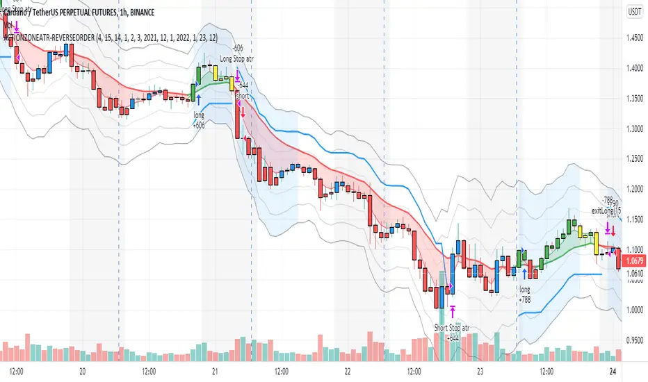
action zone - ATR stop reverse order strategy v0.1 by 9nckACTION ZONE-ATR MOD v0.1 DOCUMENTATION
Overview
This tradingview pine script strategy is mainly created to enrich my coding skill. It is a combination of “CDC-ACTIONZONE” and my personal studies of trading techniques in various sources e.g.book, course or blog. This strategy purposefully built to connect with my automatic trading bot. However, It will be very useful to aid your trading routine by diminishing mental distraction which possibly leads to bad trades.
How does it work?
This strategy will do a basic simple thing that most traders do by creating entry signals on both sides long/short and also set the stop loss. Furthermore, It will also reverse the order (from long to short and vice versa (if long/short conditions are met). Finally, it will recalculate the stop loss/take profit price in every complete bar to increase the chance of winning and limit our loss.
Entry rules(Long/Short)
If you have no open order, an order will be created when a fast EMA crosses(up(long)/down(short) the slow EMA(It’s as simple as that).
If you have an open order, the current order will be (sold if long, covered if short) and the opposite side order will be created.
Exit and Reverse rules(Long/Short)
If fast EMA cross (DOWN(long), UP(short)), the current order will be closed, THE OPPOSITE SIDE ORDER WILL ALSO BE CREATED.
Risk management
FLEX STOP PRICE : initial value will be set at the bar which order created. It is a fast ema (+/-) MIDDLE ATR value.
If MIDDLE ATR value rises, it will be our new stop price.
If MIDDLE ATR value falls, stop price unchanged
If Price OVERBOUGHT(long)/SOLD(short), LOW of that bar will be a new stop price.
Minimum position hold period
In order to eliminate risk of repeatedly open, close orders in sideway trends. Minimum hold period must be passed to start exit our position. However, It always respects stop loss prices. The value refers to the number of bars.
MUST READ!!!
This strategy uses only MARKET ORDER. If you trade with a bot, make sure you choose only enormous market cap tokens.
This strategy is bi-direction strategy. It will work best in the DERIVATIVE market.
It was initially designed to compete in the cryptocurrency market which has very high volume and volatility.
I only use this strategy in 1HR (acceptable change rate, optimum trade frequency)
How (should) we use it?
Choose crypto future pairs (recommend only top 10-15 market volume pairs in Binance, let’s say 1000M+ trade value)
Choose your time frame (1H is strongly recommended)
Setup your portfolio profile (Setting->Properties) such as Initial cap, order size, commission. DO NOT USE CAL ON EVERY TICK IT WILL CAUSE REPAINTING AND YOUR CAPITAL IS BLEEDING !!!
BACKTEST FIRST!! Back test is a combination of art, math and statis(and a bit of luck). You can apply to train and test methods or whatever you are familiar with. In my opinion, your test period should include UPTREND, SIDEWAY, DOWNTREND. Fine tune fast, slow ema first(my best ema length of 1H timeframe around 7-10, 17-22). Try to eliminate fault breakout trade and use other options only necessary. Hopefully we can use automatic optimization on Pine Script soon.
Don’t forget to turn off using a specific backtest date option to start your strategy.A
THIS IS NOT A PERFECT (OR EVEN PROFITABLE) STRATEGY. USE AT YOUR OWN RISK AND TRADE RESPONSIBLY. DYOR DUDE.
72s Strat: Backtesting Adaptive HMA+ pt.1This is a follow up to my previous publication of Adaptive HMA+ few months ago, as a mean to provide some kind of initial backtesting tools. Which can be use to explore many possible strategies, optimise its settings to better conform user's pair/tf, and hopefully able to help tweaking your general strategy.
If you haven't read the study or use the indicator, kindly go here first to get the overall idea.
The first strategy introduce in this backtest is one most basic already described in the study; buy/sell is when movement is there and everything is on the right side; When RSI has turned to other side, we can use it as exit point (if in profit of course, else just let it hit our TP/SL, why would we exit before profit). Also, base on RSI when we make entry, we can further differentiate type of signals. --Please check all comments in code directly where the signals , entries , and exits section are.
Second additional strategy to check; is when we also use second faster Adaptive HMA+ for exit. So this is like a double orders on a signal but with different exit-rule (/more on this on snapshots below). Alternatively, you can also work the code so to only use this type of exit.
There's also an additional feature which you can enable its visuals, the Distance Zone , is to help measuring price distance to our xHMA+. It's just a simple atr based envelope really, I already put the sample code in study's comment section, but better gonna update it there directly for non-coder too, after this.
In this sample I use Lot for order quantity size just because that's what I use on my broker. Also what few friends use while we forward-testing it since the study is published, so we also checked/compared each profit/loss report by real number. To use default or other unit of measurement, change the entry code accordingly.
If you change your order size, you should also change the commission in Properties Tab. My broker commission is 5 USD per order/lot, so in there with example order size 0.1 lot I put commission 0.5$ per order (I'll put 2.5$ for 0.5 lot, 10$ for 2 lot, and so on). Crypto usually has higher charge. --It is important that you should fill it base on your broker.
SETTINGS
I'm trying to keep it short. Please explore it further again. (Beginner should also first get acquaintance with terms use here.)
ORDERS:
Base Minimum Profit Before Exit:
The number is multiplier of ongoing ATR. Means that when basic exit condition is met, algo will check whether you're already in minimum profit or not, if not, let it still run to TP or SL, or until it meets subsequent exit condition, then it will check again.
Default Target Profit:
Multiplier of ATR at signal. If reached before any eligible exit condition is met, exit TP.
Base StopLoss Point:
You can change directly in code to use other like ATR Trailing SL, fix percent SL, or whatever. In the sample, 4 options provided.
Maximum StopLoss:
This is like a safety-net, that if at some point your chosen SL point from input above happens to be exceeding this maximum input that you can tolerate, then this max point is the one will be use as SL.
Activate 2nd order...:
The additional doubling of certain buy/sell with different exits as described above. If enable, you should also set pyramiding to at least: 2. If not, it does nothing.
ADAPTIVE HMA+ PERIOD
Many users already have their own settings for these. So in here I only sample the default as first presented in the study. Make it to your adaptive.
MARKET MOVEMENT
(1) Now you can check in realtime how much slope degree is best to define your specific pair/tf is out of congestion (yellow) area. And (2) also able to check directly what ATR lengths are more suitable defining your pair's volatility.
DISTANCE ZONE
Distance Multiplier. Each pair/tf has its own best distance zone (in xHMA+ perspective). The zone also determine whether a signal should appear or not. (Or what type of signal, if you wanna go more detail in constructing your strategy)
USAGE
(Provided you already have your own comfortable settings for minimum-maximum period of Adaptive HMA+. Best if you already have backtested it manually too and/or apply as an add-on to your working strategy)
1. In our experiences, first most important to define is both elements in the Market Movement Settings . These also tend to be persistent for whole season since it's kinda describing that pair/tf overall behaviour. Don't worry if you still get a low Profit Factor here, but by tweaking you should start to see positive changes in one of Max Drawdown and Net Profit, or Percent Profitable.
2. Afterwards, find your pair/tf Distance Zone . When optimising this, what we seek is just a "not to bad" equity curves to start forming. At least Max Drawdown should lessen more. Doesn't have to be great already, but should be better, no red in Net Profit.
3. Then go manage the "Trailing Minimum Profit", TP, SL, and max SL.
4. Repeat 1,2,3. 👻
5. Manage order size, commission, and/or enable double-order (need pyramiding) if you like. Check if your equity can handle max drawdown before margin call.
6. After getting an acceptable backtest result, go to List of Trades tab and find the biggest loss or when many sequencing loss in a row happened. Click on it to go to exact point on chart, observe why the signal failed and get at least general idea how it can be prevented . The rest is yours, you should know your pair/tf more than other.
You can also re-explore your minimum-maximum period for both Major and minor xHMA+.
Keep in mind that all numbers in Setting are conceptually in a form of range . You don't want to get superb equity curves but actually a "fragile" , means one can easily turn it to disaster just by changing only a fraction in one/two of the setting.
---
If you just wanna test the strength of the indicator alone, you can disable "Use StopLoss" temporarily while optimising settings.
Using no SL might be tempting in overall result data in some cases, but NOTE: It is not recommended to not using SL, don't forget that we deliberately enter when it's in high volatility. If want to add flexibility or trading for long-term, just maximise your SL. ie.: chose SL Point>ATR only and set it maximum. (Check your max drawdown after this).
I think this is quite important specially for beginners, so here's an example; Hypothetically in below scenario, because of some settings, the buy order after the loss sell signal didn't appear. Let's say if our initial capital only 1000$ using leverage and order size 0,5 lot (risky position sizing already), moreover if this happens at the beginning of your trading season, that's half of account gone already in one trade . Your max SL should've made you exit after that pumping bar.
The Trailing Minimum Profit is actually look like this. Search in the code if you want to plot it. I just don't like too many lines on chart.
To maximise profit we can try enabling double-order. The only added rule coded is: RSI should rising when buy and falling when sell. 2nd signal will appears above or below default buy/sell signal. (Of course it's also prone to double-loss, re-check your max drawdown after. Profit factor play its part in here for a long run). Snapshot in comparison:
Two default sell signals on left closed at RSI exit, the additional sell signal closed later on when price crossover minor xHMA+. On buy side, price haven't met our minimum profit when first crossunder minor xHMA+. If later on we hit SL on this "+buy" signal, at least we already profited from default buy signal. You can also consider/treat this as multiple TP points.
For longer-term trading, what you need to maximise is the Minimum Profit , so it won't exit whenever an exit condition happened, it can happen several times before reaching minimum profit. Hopefully this snapshot can explain:
Notice in comparison default sell and buy signal now close in average after 3 days. What's best is when we also have confirmation from higher TF. It's like targeting higher TF by entering from smaller TF.
As also mention in the study, we can still experiment via original HMA by putting same value for minimum-maximum period setting. This is experimental EU 1H with Major xHMA+: 144-144, Flat market 13, Distance multiplier 3.6, with 2nd order activated.
Kiwi was a bit surprising for me. It's flat market is effectively below 6, with quite far distance zone of 3.5. Probably because I'm using big numbers in adaptive period.
---
The result you see in strategy tester report below for EURUSD 15m is using just default settings you see in code, as follow:
0,1 lot for each order (which is the smallest allowed by my broker).
No pyramiding. Commission: 0.5 usd per order. Slippage: 3
Opening position is only using basic strategy #1 (RSI exit). Additional exit not activated.
Minimum Profit: 1. TP: 3.
SL use: Half-distance zone. Max SL: 4.5.
Major xHMA+: 172-233. minor xHMA+: 89-121
Distance Zone Multiplier: 2.7
RSI: Standard 14.
(From our forward-testing, the difference we get from net profit is because of the spread, our entry isn't exactly at the close/open price. Not so much though, but not the same. If somebody can direct me to any example where we can code our entry via current bid/ask price, that would be awesome!)
It's already a long post (sorry), think I'm gonna pause here. Check out the code :)
---
DISCLAIMER: Past performance is no guarantee of future results , and so on.. you know the drill ;)
Please read whole description first before using, don't take 1-2 paragraph and claim it's the whole logic, you are responsible of your own actions and understanding.

MACD Price Projected Bands [MPPB] Strategy for NIFTY / BTC 2 minMACD Price Projected Bands is an intraday NON REPAINTING Strategy to be used over BTCUSD and NIFTY on 2mins charts for optimum results!!
How the Strategy works
The strategy uses MACD with standard configuration as its main component.
The adaptive Bands are calculated over the MACD lookback, and MACD crosses of the adaptive bands are projected over the Price for creating a decision logic
A cyclic Trend Filter is used to calculate the Optimum Entry and Exit Points for the Strategy,
Levels are also plotted over the price projected bands for better visualisation of the targets!
What is used !
Macd_config : { fast:12 , slow:26 , signal:9 }
Lookback Length : 55
The Strategy has Provision for Alerts
You get Two signals
1. MPPBS Buy Signal
2. MPPBS Sell Signal
How the Visual Target System Works and How to trade Using this Strategy
An Adaptive Projected Band is constructed using MACD for traders to get Visual inputs regarding targets!!
The Trading Methodologies are in below Charts
For Short Trades
For Long Trades
Strategy Configurations for Backtest
For Englishmen!
The Backtesting Rules in the Strategy calculates only when order gets filled, the basic pyramiding in the strategy is set to 1, i.e The maximum number of entries allowed in the same direction is set to 1,
Also we trade only 1 quantity of the security with initial capital of 100000USD, and The commission type used in the strategy is set to 0.05 USD that means we pay 0.05USD as commissions in every trade!
For Coders!
{
calc_on_order_fills=true,
pyramiding=1,
default_qty_type=strategy.fixed,
default_qty_value=1,
initial_capital=100000,
currency=currency.USD,
commission_type= strategy.commission.cash_per_order,
commission_value = 0.05
}
How can you get access
Only do private message to me, donot use comment box for requesting access!

Self-Optimising MACD (Experimental)Hi guys, just thought I'd share a small part of an idea i've been working on.
One of the biggest problems with algo trading is optimisation and finding a way to constantly adapt to the market conditions as time unfolds.
First of all... You should NEVER EVER trade just using a MACD, including this study, and I only produced this script in a small amount of time, so make sure you backtest it properly before using it. When backtesting, it is my advice that your sample size should be at least 5000 trades, but I recommend 10000 in order to get sufficient statistical significance.
Also, I am not a financial advisor, and any trading based decisions are your sole responsibility.
Anyways...
This script is simple... it simply uses 4 different MACD's and tracks their profit/loss and automatically uses the one with the most historical profit at any given time to execute a trade. The type of MACD will obviously change as market states fluctuate.
Included are : Hull MACD, Ema MACD, Sma MACD and VWMA Macd.
You can adjust all four of their settings to your desire.
The trade execution is simple and definitely flawed... it simply tracks the MACD when it has a crossover for long, and then the opposite for short.
The green line represents the performance of the top MACD for Longs at any given time. This line refreshes once a year, and where it is in relation to price, reflects how profitable it has been I.e - the higher it is the better.
The Red line represents the performance on the Short side, and again, it reflects profit/loss, but this time the LOWER the line is in relation to price the better.
There is no exit strategy in place! This is why I do NOT recommend trading off this script alone, but to use it as a tool to help optimise your choice of MACD.
However, your exit strategy could change your optimal choice of MACD, so keep that in mind.
The lookback period represents how far the script will track the performance at any given time. This will change your results. The longer the period, the more it will show long term success and vice versa.
This optimisation process could be done with different indicators, moving averages, or even multiple strategies to find the most statistically viable option at any given time... if you wish to have this process coded into your strategies or indicators, message me.
Enjoy.

[STRATEGY] Moving Average CrossoverHello friends,
This is a comprehensive backtesting engine for Moving Average crossover strategies, supporting over 63 types of moving averages and filters. It allows you to test, compare, and optimize crossover behaviors between any two moving averages with flexible profit and risk management tools.
Built upon the Moving Average Crossover foundation, this advanced version lets you manually backtest more than 4096 combinations of moving average types. When combined with customizable periods, take-profits, and stop-loss levels, the total number of possible configurations becomes virtually unlimited.
🛠 How It Works
The system tests crossovers between two selected moving averages, with full control over their types, lengths, and trading direction. Integrated bracket settings enable dynamic take-profit, stop-loss, and trailing-stop management using units such as % , ATR , points , pips , or ticks .
You can restrict backtesting to a custom date range for focused performance evaluation or run it across the instrument’s full history.
🔥 Key Features
Supports 63+ moving average and filter types — including algorithms by Ehlers , Jurik , Kaufman , Apirine , Tillson , and Dürschner
Customizable MA types, periods, and strategy direction
Full-featured bracket control: TP, SL, and TSL in ATR, %, points, pips, or ticks
Backtest window customization (start, end, or range)
Direction filter: Longs only, Shorts only, or Both
Dynamic trade labeling and color-coded visualization
Option to exit only at TP, SL, or TSL
If you'd like access or have any questions, feel free to reach out to me directly via DM.
👋 Good luck and happy trading!
Script a pagamento

MAMA (Ehlers) MESA Adaptive Moving AverageMAMA ( Ehlers ) MESA Adaptive Moving Average:
What it is and how it works
MESA Phasor is the most advanced futures trading program on the market!
MESA Phasor derives its name from the sinewave generator you probably recall from your high school trigonometry class. As you can see in the diagram, the rotating phasor generates a sine wave in the time domain, visualized as a shadow from the arrow tip of the phasor on the vertical axis. A cycle is completed on each full rotation of the phasor. The angle of the phasor increases at a constant rate, and is reset to zero when 360 degrees of rotation have been achieved. The idea of the trading system is to buy low at the valley of the sine wave , when phasor passes the lower angle, and to sell short at the crest of the sine wave , when the phasor passes the upper angle. Now the trade entries and exits are defined in terms of angles, which are in the frequency domain. Therefore, trading decisions are removed from waveform vagaries in the time domain. This means that the trading decisions are robust across various futures contracts and across all kinds of market conditions.
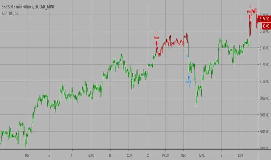
Adaptive Price Zone Backtest The adaptive price zone (APZ) is a volatility-based technical indicator that helps investors
identify possible market turning points, which can be especially useful in a sideways-moving
market. It was created by technical analyst Lee Leibfarth in the article “Identify the
Turning Point: Trading With An Adaptive Price Zone,” which appeared in the September 2006 issue
of the journal Technical Analysis of Stocks and Commodities.
This indicator attempts to signal significant price movements by using a set of bands based on
short-term, double-smoothed exponential moving averages that lag only slightly behind price changes.
It can help short-term investors and day traders profit in volatile markets by signaling price
reversal points, which can indicate potentially lucrative times to buy or sell. The APZ can be
implemented as part of an automated trading system and can be applied to the charts of all tradeable assets.
WARNING:
- For purpose educate only
- This script to change bars colors.
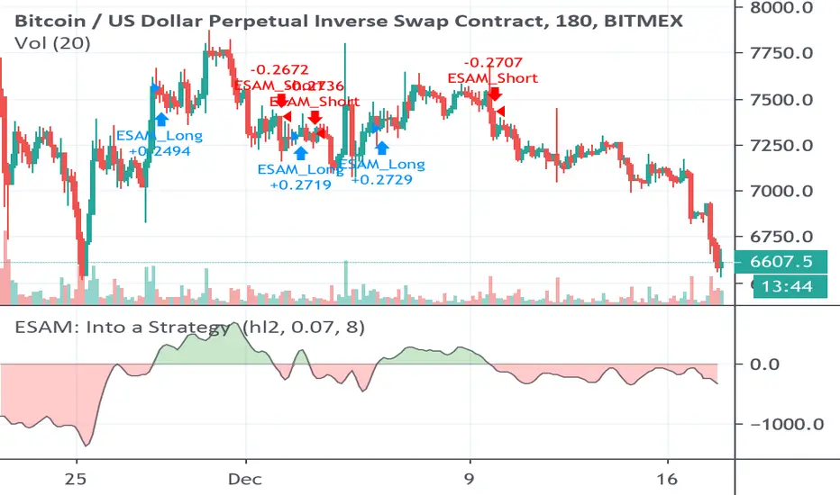
Strategy based on Ehlers Smoothed Adaptive Momentum [LazyBear]Strategy based on Ehlers Smoothed Adaptive Momentum (ESAM) indicator by LazyBear, slightly improved.
Indicator itself was developed and described by John F. Ehlers in his book "Cybernetic Analysis for Stocks and Futures" (2004, Chapter 12: Adapting to the Trend).
Backtesting: XBTUSD (Bitmex): 2h, 3h, 4h
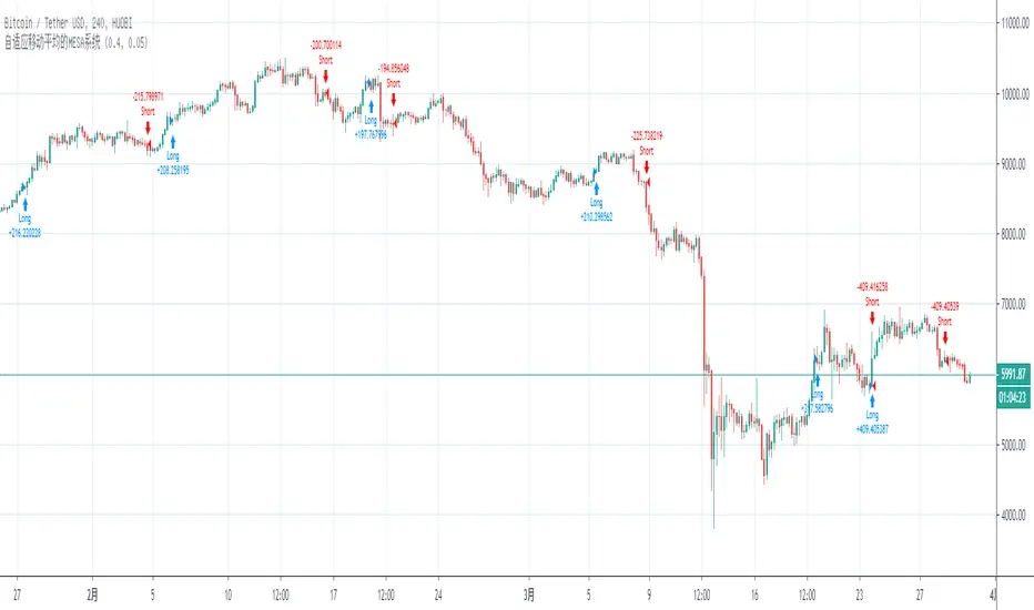
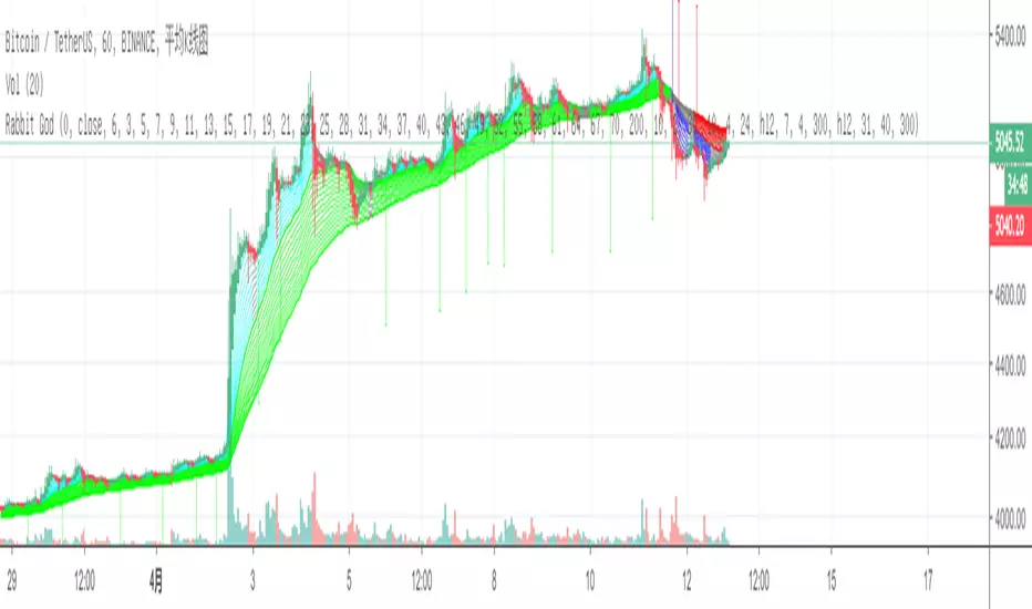
Trend tracking strategy of proprietary traders-RabbitThis is my latest strategy integration. It is a combination of trend tracking strategy and visualization trend. I believe it will bring you a clear trend discrimination and relatively reliable trading signal hints.
(Note: This strategy parameter has special parameter debugging and Optimization for BTC1h/BIANACE Heikin-ashi chart. It works best here. Other trade pairs or parameter versions of investment targets will be published specially if necessary.)
Statement of strategy concept:
The concept of strategy is trend tracking. The formation and continuation of trend is the product of speculation market for thousands of years. There are various strategies including CTA trend strategy, shock regression strategy, grid strategy, Martin strategy, Alpha strategy and so on. These strategies have their own merits just like different schools of Chinese knight-errant. Choose one, a master is not able to do hundreds of tricks, but to practice one trick thousands of times.
Every strategy has its own right and wrong. Trading is not violence, but a process of advancing, retreating, and making profits steadily. Therefore, the use of trend tracking strategy must overcome greed in human nature, profit and loss homology, dare to bear the shock of withdrawal in order to make a big profit when the real trend arrives. (Of course, this strategy has largely avoided filtering shocks, which will be explained later.)
Policy-building instructions:
Any trend tracking strategy can produce good results when there is a trend, so judging whether a trend strategy is good or bad depends on its withdrawal performance when it is shaking. This CTA trend tracking strategy uses Kauffman adaptive algorithm, fractal adaptive dimension, self-research algorithm and other tools, and has largely avoided filtering the signal in the shock without delay to follow the trend.
New version of the note:
The latest version adds the trend drawing of negativity, which can clearly distinguish the rising or falling or oscillating trend. However, the algorithm of strategy signal has no direct relationship with trend color. Trend color helps you to distinguish trend, and point signal helps you to refer to trade. This strategy is only a simple trading signal, risk control, warehouse management also need manual operation.
(Note: This strategy parameter has special parameter debugging and Optimization for BTC1h/BIANACE Heikin-ashi chart. It works best here. Other trade pairs or parameter versions of investment targets will be published specially if necessary.)
Good luck to all of you and a smooth deal.~

Best Rabbit Strategy fiterResults after a long period of research
This strategy uses CTA Trend Tracking Strategy, which is given to the person who is close to you. And add filter with fractal dimension. Please note that any strategy is correct and wrong. Please accept the loss list calmly so as to make a big profit when the trend comes.
It works better with Heikinashi chart.
Adaptive Zero Lag EMA v2This is my most successful strategy to date! Please enjoy and join the Open Source movement by sharing your code and ideas online!
OPERATING PRINCIPLE
The strategy is based on Ehlers idea that any indicator can be turned into a signal-producing trade system through smoothing and other filtering processes.
In fact, I'm using his Zero Lag EMA (ZLEMA) as a baseline indicator as well as some code snippets he has made public (1). God bless open source!
Next, I've provided the option to use an Instantaneous Frequency Measurement (IFM) method, which will adaptively choose the best period for the ZLEMA (2)
I've written other studies that use the differential calculus approximations for IFM, so it was only natural to include them in this strategy.
The primary two are Cosine IFM (3) and In-phase Quadrature IFM (4). You can also find an indicator with both plotted and the ability to average them together, as one IFM prefers long periods and the other short. (5)
BEFORE WE BEGIN
1. This strategy only runs on "normal" FX pairs (EURUSD, GBPJPY, AUDUSD ...) and will fail on Metals or Commodities.
Cryptos are largely untested.
2. Please run it on these time frames: M15 to D.
Anything outside this range will likely fail.
HOW TO USE AND SUCCEED
1. If the Default settings don't produce good results right off the bat, then lower gain limit to 1 or 2 and threshold to 0.01.
2. Test each setting under adaptive method . If you want to leave it Off , then I'd recommend using some kind of IFM (see my links below) to
discover the most efficient period to use.
3. Once you have the best adaptive method chosen, begin incrementing gain limit until you find a nice balance between profit factor (PF) and drawdown.
4. Now, begin incrementing threshold . The goal is to have PF above 2 and a drawdown as low as possible.
5. Finally, change the source ! Typically, close is the best option, but I have run into cases where high
yielded the highest returns and win rate.
6. Sit back, relax, and tweak the risk until you're happy with the return and drawdown amounts.
ADVANCED
You may need to adjust take profit (TP) points and stop loss (SL) points to create the best entry possible. Don't be greedy! You'll likely have poor
results if the TP is set to 300 and SL is 50.
If you are trading a pair that has a long Dominant Cycle Period , then you may increase Max Period to allow the IFM
to accept longer periods. Any period above the Max Period will be rejected. This may increase lag time!
Cheers and good luck trading!
-DasanC
PS - This code doesn't repaint or have future-leak, which was present in Pinescript v2.
PPS - Believe me! These returns are typical! Sometimes you must push aside the "if it's too good to be true..." mindset that society has ingrained in you.
Do you really believe the most successful pass up opportunities before investigating them? ;)
(1) Ehlers & Ric Zero Lag EMA
(2) Measuring Cycles by Ehlers
(3) Cosine IFM
(4) Inphase Quadrature IFM
(5) Averaging IFM

Adaptive Zero Lag EMA Strategy [Ehlers + Ric]Behold! A strategy that makes use of Ehlers research into the field of signal processing and wins so consistently, on multiple time frames AND on multiple currency pairs.
The Adaptive Zero Lag EMA (AZLEMA) is based on an informative report by Ehlers and Ric .
I've modified it by using Cosine IFM, a method by Ehlers on determining the dominant cycle period without using fast-Fourier transforms
Instead, we use some basic differential equations that are simplified to approximate the cycle period over a 100 bar sample size.
The settings for this strategy allow you to scalp or swing trade! High versatility!
Since this strategy is frequency based, you can run it on any timeframe (M1 is untested) and even have the option of using adaptive settings for a best-fit.
>Settings
Source : Choose the value for calculations (close, open, high + low / 2, etc...)
Period : Choose the dominant cycle for the ZLEMA (typically under 100)
Adaptive? : Allow the strategy to continuously update the Period for you (disables Period setting)
Gain Limit : Higher = faster response. Lower = smoother response. See for more information.
Threshold : Provides a bit more control over entering a trade. Lower = less selective. Higher = More selective. (range from 0 to 1)
SL Points : Stop Poss level in points (10 points = 1 pip)
TP Points : Take Profit level in points
Risk : Percent of current balance to risk on each trade (0.01 = 1%)
www.mesasoftware.com
www.jamesgoulding.com(Measuring%20Cycles).doc
Adaptive Trend OscilatorAdaptive strategy for strong move starting points. When it capture signal stay in that direction until lost momentum or get a counter signal