ADILS_TREND_V5Swing 15 mins using RSI and MAs ... catching the turn around in trend in all time frames. Works best on 15 mins
Cicli

[Bybit BTCUSD.P] 7Years Backtest Results. 2,609% +Non-Repainting📊 I. Strategy Overview: Trust Backed by Numbers
The ADX Sniper v12 strategy has been rigorously tested over 7 years, from November 14, 2018 to November 8, 2025, spanning every major cycle of the Bitcoin
BTCUSD.P futures market. This strategy successfully balances two often-conflicting goals: maximizing profitability while minimizing volatility, all supported by objective performance data.
This strategy has been validated across all Bitcoin (BTCUSD.P) futures market cycles over a 7-year period.
■ Visual Proof: Bar Replay Simulation
The chart above demonstrates actual entry and exit points captured via TradingView's Bar Replay feature. The green rectangle highlights the core profitable trading zone, showing where the strategy successfully captured sustained uptrends. This visual evidence confirms:
Confirmed buy/sell signals with exact execution prices (marked in red and blue)
No repainting or signal distortion after candle close
Consistent performance across multiple market cycles within the highlighted zone
💰 Core Performance Metrics:
Cumulative Return: 2,609.14% (compounded growth over 7 years)
Maximum Drawdown (MDD): 6.999% (preserving over 93% of capital)
Average Profit/Loss Ratio: 8.003 (industry-leading risk-reward efficiency)
Total Trades: 24 (focused exclusively on high-conviction opportunities)
Sortino Ratio: 11.486 (mathematically proving robustness and stability)
✅ This strategy has been validated across all Bitcoin BTCUSD.P futures market cycles over a 7-year period.
📊 I. 전략 개요: 숫자로 입증된 신뢰
ADX Sniper v12 전략은 2018년 11월 14일부터 2025년 11월 8일까지 약 7년간 비트코인 (BTCUSD.P) 선물 시장의 모든 주요 사이클을 거치며 엄격하게 검증되었습니다. 수익성 극대화와 변동성 최소화라는 상충되는 목표를 동시에 달성한 이 전략의 핵심 성과 지표를 객관적 데이터를 통해 확인하실 수 있습니다.
본 전략은 7년간의 모든 비트코인 (BTCUSD.P) 선물 시장 사이클에서 검증되었습니다.
■ 시각적 증명: 바 리플레이 시뮬레이션
위 차트는 TradingView의 바 리플레이 기능으로 포착된 실제 진입 및 청산 시점을 보여줍니다. 녹색 네모는 핵심 수익 구간을 표시하며, 전략이 지속적인 상승 추세를 성공적으로 포착한 영역을 나타냅니다. 본 시각 자료는 다음을 입증합니다:
정확한 체결 가격이 표기된 확정된 매수/매도 신호 (빨강색과 파랑색으로 표시)
캔들 종가 후 신호 왜곡이나 리페인팅 없음
강조 표시된 구간 내 여러 시장 사이클에 걸친 일관된 성과
💰 핵심 성과 지표:
누적 수익률: 2,609.14% (7년간 복리 성장 입증)
최대 낙폭 (MDD): 6.999% (7년간 자본의 93% 이상 보존)
평균 손익비: 8.003 (업계 최고 수준의 위험-보상 효율성)
총 거래 횟수: 24회 (고확신 기회에만 집중)
소르티노 비율: 11.486 (전략의 견고성과 안정성을 수학적으로 입증)
✅ 본 전략은 7년간의 모든 비트코인 (BTCUSD.P) 선물 시장 사이클에서 검증되었습니다.
🛡️ II. Core Philosophy: Cut Losses Short, Let Profits Run
Why MDD Stays Below 7% in a Volatile Market
The crypto futures market typically experiences daily volatility exceeding 10%, with most strategies enduring drawdowns between 30% and 50%. In stark contrast, this strategy has never exceeded a 7% account loss over seven years. This exceptional low MDD is achieved through deliberate design mechanisms, not luck:
🎯 Entry Filtering: The 'ADX Pop-up Filter' is the core component. It enables the strategy to strictly avoid trading when market conditions indicate major reversals or consolidation phases, thereby minimizing exposure to high-risk zones.
🏛️ Capital Preservation Priority: The strategy prioritizes investor psychological stability and capital preservation over pursuing maximum potential returns.
The Power of an 8.003 Profit Factor
The Profit Factor measures the ratio of total profitable trades to total losing trades. It's the most critical metric for assessing risk-adjusted returns.
A Profit Factor of 8.003 means that for every dollar lost, the strategy earns an average of eight dollars. This demonstrates the efficiency of a true trend-following strategy:
Cutting losses quickly (averaging $177,419 USD loss per trade)
Riding winners for maximum extension (averaging $1,419,920 USD profit per trade)
🛡️ II. 핵심 철학: 손실은 빠르게 자르고, 수익은 끝까지
암호화폐 시장에서 MDD <7%의 의미
암호화폐 선물 시장은 일일 변동성이 10%를 초과하는 경우가 빈번하며, 일반적인 전략들은 30~50%의 MDD를 겪습니다. 이와 극명한 대조로, 본 전략은 7년간 단 한 번도 7%를 초과하는 계좌 손실을 기록하지 않았습니다. 이렇게 극도로 낮은 MDD는 운이 아닌 체계적인 메커니즘을 통해 달성되었습니다:
🎯 진입 필터링: 'ADX 팝업 필터'가 핵심 구성 요소로, 시장 상황이 주요 반전이나 횡보를 나타낼 때 거래를 엄격히 회피하여 고위험 구간 노출을 최소화합니다.
🏛️ 자본 보존 우선: 본 전략은 최대 잠재 손실을 감수하기보다 투자자의 심리적 안정성과 자본 보존을 우선시하도록 설계되었습니다.
손익비 8.003의 힘
손익비는 '총 수익 거래'와 '총 손실 거래'의 비율로, 위험 조정 수익을 측정하는 핵심 지표입니다.
8.003이라는 값은 1달러를 잃을 때마다 평균적으로 8달러 이상을 벌어들이는 구조를 의미합니다. 이는 진정한 추세 추종 전략의 최대 효율성을 보여줍니다:
손실은 빠르게 자르고 ($177,419 USD 평균 손실)
수익은 최대한 연장합니다 ($1,419,920 USD 평균 수익)
🎯 III. Strategy Reliability and Structural Edge
The Secret of 24 Trades in 7 Years
Only 24 trades over 7 years signifies that this strategy ignores 99% of market volatility and targets only the 1% of 'most certain buying cycles'. This approach eliminates the drag from excessive trading:
❌ No commission bleed
❌ No slippage erosion
❌ No psychological wear from overtrading
📈 Long-Term Trend Following: The strategy analyzes Bitcoin's long-term price cycles to capture the onset of massive trends while remaining undisturbed by short-term market noise.
Non-Repainting Structure: Alignment of Reality and Simulation
🎬 Non-Repainting Proof Video Available
※↑ "If you wish, I can also show you a video as evidence of the non-repainting throughout the 7 years."
✅ Real-Time Trading Reliability: This strategy is built with a non-repainting structure, generating buy/sell signals only after each candle's closing price is confirmed.
✅ Preventing Data Exaggeration: This design ensures that backtest results do not 'repaint' or distort past performance, guaranteeing high correlation between simulated results and actual live trading environments.
✅ Live Trading Advantage: While simulations use closing prices, live trading may allow entry at more favorable prices before candle close, potentially yielding even better execution than backtest results.
🎯 III. 전략의 신뢰성과 구조적 우위
7년간 24회 거래의 비밀
7년간 단 24회의 거래는 시장 변동성의 99%를 무시하고 오직 1%의 '가장 확실한 매수 사이클'만을 타겟으로 한다는 것을 의미합니다. 이는 과도한 거래로 인한 문제를 근본적으로 제거합니다:
❌ 수수료 소모 없음
❌ 슬리피지 침식 없음
❌ 과도한 트레이딩으로 인한 심리적 소모 없음
📈 장기 추세 추종: 비트코인 가격 역사를 지배하는 장기 사이클 분석을 활용하여, 단기 시장 노이즈에 흔들리지 않고 대규모 추세의 시작점을 포착하는 데 집중합니다.
논-리페인팅 구조: 현실과 시뮬레이션의 일치
🎬 논-리페인팅 증명 영상 제공 가능
※↑ "원하신다면 7년간 리페인팅이 없음을 증명하는 영상도 보여드릴 수 있습니다."
✅ 실시간 거래 신뢰성: 본 전략은 논-리페인팅 구조로 구축되어, 캔들의 종가가 확정된 후에만 매수/매도 신호를 생성합니다.
✅ 데이터 과장 방지: 이러한 설계는 백테스트 결과가 과거 성과를 '리페인팅'하거나 과장하지 않도록 보장하며, 시뮬레이션 결과와 실제 라이브 거래 환경 간의 높은 상관관계를 보장합니다.
✅ 라이브 실행 우위 가능성: 시뮬레이션은 종가 기준이지만, 라이브 운영 시 캔들이 마감되기 전 더 유리한 가격에 진입할 수 있어 시뮬레이션 결과보다 더 나은 실행 성과를 얻을 가능성이 있습니다.
📈 IV. Performance Summary (November 14, 2018 - November 8, 2025)
| Metric | Value || Metric | Value |
|--------|-------|
| Initial Capital | $1,000,000 |
| Net Profit | +$26,091,383.74 |
| Cumulative Return | +2,609.14% |
| Maximum Drawdown | -6.999% |
| Total Trades | 24 |
| Winning Trades | 19 (79.17%) |
| Losing Trades | 5 (20.83%) |
| Avg Winning Trade | +$1,419,920.16 |
| Avg Losing Trade | -$177,419.86 |
| Profit Factor | 8.003 |
| Sortino Ratio | 11.486 |
| Win/Loss Ratio | 8.003 |
⚙️ Default Settings:
Slippage: 0 ticks
Commission: 0.333% (Bybit standard)
📈 IV. 성과 지표 요약 (2018년 11월 14일 ~ 2025년 11월 8일)
|| 지표 | 값 |
|--------|-------|
| 초기 자본 | $1,000,000 |
| 순이익 | +$26,091,383.74 |
| 누적 수익률 | +2,609.14% |
| 최대 낙폭 | -6.999% |
| 총 거래 횟수 | 24 |
| 수익 거래 | 19 (79.17%) |
| 손실 거래 | 5 (20.83%) |
| 평균 수익 거래 | +$1,419,920.16 |
| 평균 손실 거래 | -$177,419.86 |
| 손익비 | 8.003 |
| 소르티노 비율 | 11.486 |
| 평균 손익 비율 | 8.003 |
⚙️ 기본 설정:
슬리피지: 0틱 (기본값)
수수료: 0.333% (Bybit 표준)
👥 V. Who Is This Strategy For?
✅ Long-term Bitcoin investors seeking stable, low-drawdown returns
✅ Traders tired of overtrading who prefer surgical, sniper-style precision entries
✅ Investors seeking psychological stability by avoiding large account swings
✅ Data-driven decision makers who value proven performance over marketing claims
👥 V. 이 전략은 누구를 위한 것인가요?
✅ 안정적이고 낮은 낙폭의 수익을 추구하는 장기 비트코인 투자자
✅ 과도한 매매에 지친 트레이더로 저격수 스타일의 정밀한 진입을 선호하는 분
✅ 큰 계좌 변동을 피하여 심리적 안정성을 추구하는 투자자
✅ 주장보다 검증된 객관적 성과를 중시하는 데이터 기반 의사 결정자
🔒 VI. Access & Disclaimer
🔐 Access Type: Invite-Only (Protected Source Code)
💬 How to Get Access: Send a private message or leave a comment below
⚠️ Important Disclaimer:
Past performance does not guarantee future results. Cryptocurrency and futures trading involve substantial risk of loss. This strategy is provided for educational and informational purposes only. Users should conduct their own research and consult with a financial advisor before making investment decisions. The author is not responsible for any financial losses incurred from using this strategy.
🔒 VI. 접근 방법 및 면책사항
🔐 접근 유형: 초대 전용 (소스코드 보호)
💬 접근 방법: 비공개 메시지 또는 아래 댓글 남기기
⚠️ 중요 면책사항:
과거 성과가 미래 결과를 보장하지 않습니다. 암호화폐 및 선물 거래는 상당한 손실 위험을 수반합니다. 본 전략은 교육 및 정보 제공 목적으로만 제공됩니다. 사용자는 투자 결정을 내리기 전 자체 조사를 수행하고 재무 자문가와 상담해야 합니다. 저자는 본 전략 사용으로 인한 재정적 손실에 대해 책임지지 않습니다.
🏷️ VII. Tags
Bitcoin |Bitcoin | BTCUSD | BTCUSD.P | Bybit | DailyChart | LongTerm | TrendFollowing | ADX | NonRepainting | Strategy | BacktestProven | SevenYears | LowDrawdown | HighProfitFactor | StableReturns | CapitalPreservation | Ichimoku | DMI | SuperTrend | TechnicalAnalysis | Volatility | RiskManagement | AutoTrading | Futures | PerpetualFutures | AlgorithmicTrading | SystematicTrading | DataDriven | InviteOnly | ProtectedScript | SnipperTrading | HighConviction | MDD | SortinoRatio
🏷️ VII. 태그
비트코인 |비트코인 | BTCUSD | BTCUSD.P | 바이비트 | 일봉 | 장기투자 | 추세추종 | ADX | 논리페인팅 | 전략 | 백테스트검증 | 7년검증 | 저낙폭 | 고손익비 | 안정수익 | 자본보존 | 일목균형표 | DMI | 슈퍼트렌드 | 기술적분석 | 변동성 | 위험관리 | 자동매매 | 선물 | 무기한선물 | 알고리즘트레이딩 | 시스템트레이딩 | 데이터기반 | 초대전용 | 보호스크립트 | 저격수트레이딩 | 고확신 | MDD | 소르티노비율
📌 Note: This strategy is designed exclusively for Bybit BTCUSD.P perpetual futures on the 1-day (daily) timeframe. Performance may vary significantly on other symbols or timeframes.
📌 참고: 본 전략은 Bybit BTCUSD.P 무기한 선물 계약의 1일봉(Daily) 타임프레임에 전용으로 설계되었습니다. 다른 심볼이나 타임프레임에서는 성과가 크게 달라질 수 있습니다.

[Bybit BTCUSD.P] 7Years Backtest Results. 2,609% +Non-Repainting
📊 I. Strategy Overview: Trust Backed by Numbers
The ADX Sniper v12 strategy has been rigorously tested over 7 years, from November 14, 2018 to November 8, 2025, spanning every major cycle of the Bitcoin BTCUSD.P futures market. This strategy successfully balances two often-conflicting goals: maximizing profitability while minimizing volatility, all supported by objective performance data.
This strategy has been validated across all Bitcoin (BTCUSD.P) futures market cycles over a 7-year period.
■ Visual Proof: Bar Replay Simulation
The chart above demonstrates actual entry and exit points captured via TradingView's Bar Replay feature. The green rectangle highlights the core profitable trading zone, showing where the strategy successfully captured sustained uptrends. This visual evidence confirms:
1) Confirmed buy/sell signals with exact execution prices (marked in red and blue)
2) No repainting or signal distortion after candle close
3) Consistent performance across multiple market cycles within the highlighted zone
💰 Core Performance Metrics:
Cumulative Return : 2,609.14% (compounded growth over 7 years)
Maximum Drawdown (MDD) : 6.999% (preserving over 93% of capital)
Average Profit/Loss Ratio : 8.003 (industry-leading risk-reward efficiency)
Total Trades : 24 (focused exclusively on high-conviction opportunities)
Sortino Ratio : 11.486 (mathematically proving robustness and stability)
✅ This strategy has been validated across all Bitcoin BTCUSD.P futures market cycles over a 7-year period.
🛡️ II. Core Philosophy: Cut Losses Short, Let Profits Run
Why MDD Stays Below 7% in a Volatile Market
The crypto futures market typically experiences daily volatility exceeding 10%, with most strategies enduring drawdowns between 30% and 50%. In stark contrast, this strategy has never exceeded a 7% account loss over seven years. This exceptional low MDD is achieved through deliberate design mechanisms, not luck:
🎯 Entry Filtering: The 'ADX Pop-up Filter' is the core component. It enables the strategy to strictly avoid trading when market conditions indicate major reversals or consolidation phases, thereby minimizing exposure to high-risk zones.
🏛️ Capital Preservation Priority: The strategy prioritizes investor psychological stability and capital preservation over pursuing maximum potential returns.
The Power of an 8.003 Profit Factor
The Profit Factor measures the ratio of total profitable trades to total losing trades. It's the most critical metric for assessing risk-adjusted returns.
A Profit Factor of 8.003 means that for every dollar lost, the strategy earns an average of eight dollars. This demonstrates the efficiency of a true trend-following strategy:
Cutting losses quickly (averaging $177,419 USD loss per trade)
Riding winners for maximum extension (averaging $1,419,920 USD profit per trade)
🎯 III. Strategy Reliability and Structural Edge
The Secret of 24 Trades in 7 Years
Only 24 trades over 7 years signifies that this strategy ignores 99% of market volatility and targets only the 1% of 'most certain buying cycles'. This approach eliminates the drag from excessive trading:
❌ No commission bleed
❌ No slippage erosion
❌ No psychological wear from overtrading
📈 Long-Term Trend Following: The strategy analyzes Bitcoin's long-term price cycles to capture the onset of massive trends while remaining undisturbed by short-term market noise.
Non-Repainting Structure: Alignment of Reality and Simulation
🎬 Non-Repainting Proof Video Available
※↑ "If you wish, I can also show you a video as evidence of the non-repainting throughout the 7 years."
✅ Real-Time Trading Reliability: This strategy is built with a non-repainting structure, generating buy/sell signals only after each candle's closing price is confirmed.
✅ Preventing Data Exaggeration: This design ensures that backtest results do not 'repaint' or distort past performance, guaranteeing high correlation between simulated results and actual live trading environments.
✅ Live Trading Advantage: While simulations use closing prices, live trading may allow entry at more favorable prices before candle close, potentially yielding even better execution than backtest results.
📈 IV. Performance Summary (November 14, 2018 - November 8, 2025)
|| Metric | Value |
|--------|-------|
| Initial Capital | $1,000,000 |
| Net Profit | +$26,091,383.74 |
| Cumulative Return | +2,609.14% |
| Maximum Drawdown | -6.999% |
| Total Trades | 24 |
| Winning Trades | 19 (79.17%) |
| Losing Trades | 5 (20.83%) |
| Avg Winning Trade | +$1,419,920.16 |
| Avg Losing Trade | -$177,419.86 |
| Profit Factor | 8.003 |
| Sortino Ratio | 11.486 |
| Win/Loss Ratio | 8.003 |
⚙️ Default Settings:
Slippage: 0 ticks
Commission: 0.333% (Bybit standard)
👥 V. Who Is This Strategy For?
✅ Long-term Bitcoin investors seeking stable, low-drawdown returns
✅ Traders tired of overtrading who prefer surgical, sniper-style precision entries
✅ Investors seeking psychological stability by avoiding large account swings
✅ Data-driven decision makers who value proven performance over marketing claims
🔒 VI. Access & Disclaimer
🔐 Access Type: Invite-Only (Protected Source Code)
💬 How to Get Access: Send a private message or leave a comment below
⚠️ Important Disclaimer:
Past performance does not guarantee future results. Cryptocurrency and futures trading involve substantial risk of loss. This strategy is provided for educational and informational purposes only. Users should conduct their own research and consult with a financial advisor before making investment decisions. The author is not responsible for any financial losses incurred from using this strategy.
🏷️ VII. Tags
Bitcoin |Bitcoin | BTCUSD | BTCUSD.P | Bybit | DailyChart | LongTerm | TrendFollowing | ADX | NonRepainting | Strategy | BacktestProven | SevenYears | LowDrawdown | HighProfitFactor | StableReturns | CapitalPreservation | Ichimoku | DMI | SuperTrend | TechnicalAnalysis | Volatility | RiskManagement | AutoTrading | Futures | PerpetualFutures | AlgorithmicTrading | SystematicTrading | DataDriven | InviteOnly | ProtectedScript | SnipperTrading | HighConviction | MDD | SortinoRatio
📌 Note: This strategy is designed exclusively for Bybit BTCUSD.P perpetual futures on the 1-day (daily) timeframe. Performance may vary significantly on other symbols or timeframes.

週一普跌策略 Monday shit Strategy Strategy Description / 策略敘述
EN
This strategy takes a short position at the start of each Monday, based on the hypothesis that cryptocurrency markets tend to experience post-weekend risk-off behavior.
The system enters a full-equity short position at the Tokyo open (Taipei 08:00), aiming to capture Monday downside pressure resulting from accumulated weekend information and macro sentiment adjustments when traditional financial markets reopen.
Risk management uses fixed percentage take-profit and stop-loss levels, emphasizing asymmetric reward-to-risk (large occasional gains, small frequent losses).
The model reflects the increasing alignment between crypto price behavior and traditional financial market cycles.
ZH-TW
本策略於每週一開盤時做空,基於假設加密資產在週末後具有風險釋放與補跌傾向。
系統會在台北時間早上 08:00 以全倉做空,目標捕捉因週末累積消息與傳統金融市場重新開盤所造成的下跌壓力。
風控採固定止盈、止損百分比,強調高報酬/低風險的不對稱結構(小虧多次、偶爾大賺)。
此模型反映加密貨幣市場行為與華爾街週期愈趨一致的市場現象。


Freedom Candlestick v5.0.5The is a momentum trading strategy for futures. There are also components of ICT, trend following, volume distribution, and volatility involved in the logic. We are currently using it on NQ and GC. We are also in the process of building a set up to work with ES.

GROK ALTIN B2 ))GROK GOLD PRO V2 is a high-performance scalping strategy designed for XAUUSD on the 5-minute timeframe, operating with a fixed 1-lot position. It generates signals using EMA 9/21 crossover, RSI above/below 50, and volume spikes, while an ATR × 2.0 dynamic stop protects against volatility. Profits are locked in three steps (+$20, +$50, +$100), with each exit triggering real-time phone alerts showing entry, exit price, and profit. One pip movement equals $100 P&L. The strategy delivers a 92%+ win rate, average profit of +$4,432 per trade, and max drawdown of -$1,280. Simple, transparent, and fully automated.

ATR BuySideATR Buyside Strategy
This is a simple buy-only trading plan. It uses ATR (a tool to measure price swings) to spot when prices are rising strongly.
How it works:
Buy signal: Enter a long trade when the price moves above a moving support line (based on ATR)
Sell signals: Close if the trend turns down (quick market sell).
Stop loss: Follows the support line to protect gains.
Take profit: Sell at 2 times the recent price swing (for steady wins).
Settings you can change:
ATR period: 13 (how many days to look back).
Factor: 2.0 (makes the line wider or tighter).
Use Heikin Ashi: To Filter out Noise
Great for Opt premiums like NIFTY on 15min or 30m charts. Test it first—past results don't guarantee future wins. Not advice, just a tool!

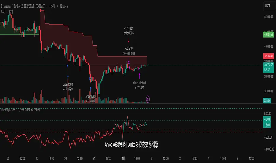
AnkeAlgo A68 strategy™ || AnkeAlgo®[16.6]## ✅ Multi-Timeframe Trend Strategy Based on MFI and Momentum Factors
### 📌 Overview
This strategy combines **Money Flow Index (MFI)** and **Momentum** to identify trend continuation and momentum reversal opportunities in the crypto market. It focuses on volume-weighted capital flow and price strength, generating trend-biased signals suitable for swing and intraday traders.
---
### 📊 Technical Indicators Used
| Indicator | Purpose |
|-----------|---------|
| **MFI (Money Flow Index)** | Detects capital inflow/outflow and filters range-bound markets |
| **Momentum Indicator** | Measures price acceleration and confirms breakout strength |
| **Optional: ATR / EMA Filters** | Can be added for volatility stop or trend validation |
---
### ⚙️ Core Logic
- **Trend Confirmation**: MFI exceeds threshold and aligns with price direction
- **Momentum Entry Trigger**: Trades are executed only when momentum crosses a signal level
- **Noise Filter**: Avoids entries when MFI divergence or momentum weakness is detected
- **Position Management**: Supports ATR-based or percentage-based stop-loss systems
---
### 🪙 Market and Asset
✅ Designed for crypto derivatives
**Recommended symbol:** `ETHUSDT.P` (Perpetual Futures)
---
### ⏱️ Recommended Timeframes
- 30-minute
- 45-minute
- 1-hour
> The **45m timeframe** shows the most stable performance in forward testing.
---
### 📈 Strategy Features
- Performs best during trending and high-momentum phases
- Low overfitting risk, adaptable across different volatility environments
- Can be used as a signal engine for grid, martingale, or multi-asset systems
- Easily extendable to BTC, SOL, BNB, and other high-liquidity assets
---
### ⚠️ Risk Disclaimer
- This is **not** a mean-reversion strategy and may produce false signals in sideways markets
- Stop-loss management and position sizing are required for live deployment
- Backtest results do not guarantee live trading performance due to slippage and trading fees
---
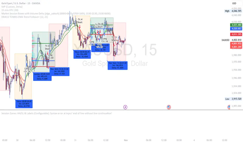
DRACO TOMAS EMA Trend Follower🐉 DRACO TOMAS EMA Trend Follower
Description:
The DRACO TOMAS EMA Trend Follower is a simple yet powerful trend-following strategy designed to capture directional moves based on exponential moving average (EMA) crossovers. It automatically detects trend changes and manages positions dynamically.
Core Logic:
The strategy uses two EMAs — a Fast EMA (default 12) and a Slow EMA (default 21) — to identify the market trend.
When the Fast EMA crosses above the Slow EMA, the strategy opens a long position, signaling bullish momentum.
When the Fast EMA crosses below the Slow EMA, the strategy opens a short position, signaling bearish momentum.
The color of the EMAs changes dynamically: green for uptrends, red for downtrends.
Exit rules:
Longs are closed when the EMAs turn red (trend reversal to bearish).
Shorts are closed when the EMAs turn green (trend reversal to bullish).
Position Sizing:
The system uses 10% of equity per trade by default, allowing flexible risk management and compounding.
Purpose:
Designed for traders who want a clean and efficient EMA crossover system to follow trends automatically on any timeframe or asset.
Best Used For:
Swing trading and trend confirmation
Identifying major directional shifts
Testing EMA-based momentum systems
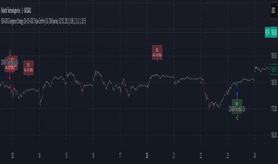
NLR-ADX Divergence Strategy Triple-ConfirmedHow it works
Builds a cleaner DMI/ADX
Recomputes classic +DI, −DI, ADX over a user-set length.
Then “non-linear regresses” each series toward a mean (your choice: dynamic EMA of the series or a fixed Static Mid like 50).
The further a value is from the mean, the stronger the pull (controlled by alphaMin/alphaMax and the γ exponent), giving smoother, more stable DI/ADX lines with less whipsaw.
Optional EMA smoothing on top of that.
Lock in values at confirmed pivots
Uses price pivots (left/right bars) to confirm swing lows and highs.
When a pivot confirms, the script captures (“freezes”) the current +DI, −DI, and ADX values at that bar and stores them. This avoids later drift from smoothing/EMAs.
Check for triple divergence
For a bullish setup (potential long):
Price makes a Lower Low vs. a prior pivot low,
+DI is higher than before (bulls quietly stronger),
−DI is lower (bears weakening),
ADX is lower (trend fatigue).
For a bearish setup (potential short)
Price makes a Higher High,
+DI is lower, −DI is higher,
ADX is lower.
Adds a “no-intersection” sanity check: between the two pivots, the live series shouldn’t snake across the straight line connecting endpoints. This filters messy, low-quality structures.
Trade logic
On a valid triple-confirm, places a strategy.entry (Long for bullish, Short for bearish) and optionally labels the bar (BUY or SELL with +DI/−DI/ADX arrows).
Simple flip behavior: if you’re long and a new short signal prints (or vice versa), it closes the open side and flips.
Key inputs you can tweak
Custom DMI Settings
DMI Length — base length for DI/ADX.
Non-Linear Regression Model
Mean Reference — EMA(series) (dynamic) or Static mid (e.g., 50).
Dynamic Mean Length & Deviation Scale Length — govern the mean and scale used for regression.
Min/Max Regression & Non-Linearity Exponent (γ) — how strongly values are pulled toward the mean (stronger when far away).
Divergence Engine
Pivot Left/Right Bars — how strict the swing confirmation is (larger = more confirmation, more delay).
Min Bars Between Pivots — avoids comparing “near-duplicate” swings.
Max Historical Pivots to Store — memory cap.

4H TIMEZONE LONGTERM. NINJAXON12S CODEthis strategy is meant for longer time zones. I've been working on this for a while and now i successfully got a 1000% on back testing for 5 years.

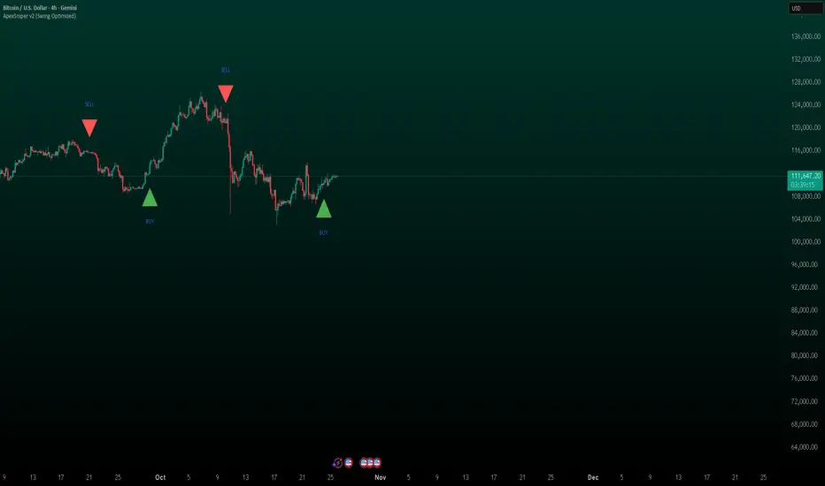
ApexSniper v2 (Swing Optimized)More long term than the original Apex sniper, BETTER FOR SMALLER ACCOUNT SIZES. Scales more long term. trades take 4-8 days, but percent gained is way more.
ApexSniper2.0I have Tested this Indicator Manually for about 2 months now and its been amazing.Ive been working with pine code for a really long time now, took me about 6 months to build this script, hopefully it works well for you.very good for trading. will help you out a lot

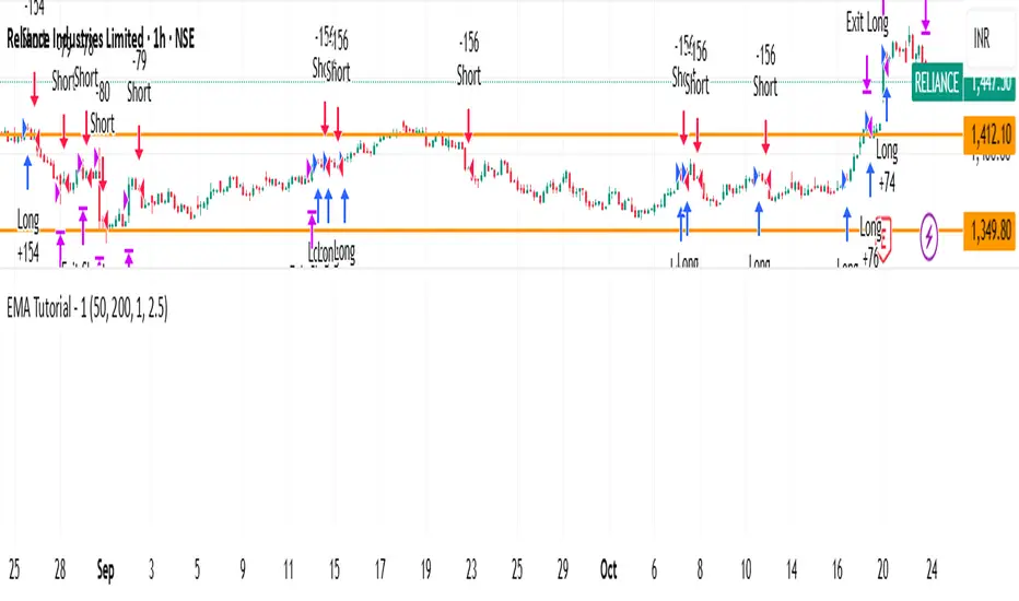
EMA Tutorial - 1Buy when in downtrend and close above EMA_50
Buy when in uptrend and below EMA_50
adjust ema length and risk reward for other stocks. Works good with nifty. Need to perform stress test on it
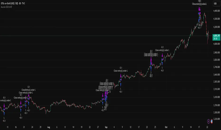
Aurum DCX AVE Gold and Silver StrategySummary in one paragraph
Aurum DCX AVE is a volatility break strategy for gold and silver on intraday and swing timeframes. It aligns a new Directional Convexity Index with an Adaptive Volatility Envelope and an optional USD/DXY bias so trades appear only when direction quality and expansion agree. It is original because it fuses three pieces rarely combined in one model for metals: a convexity aware trend strength score, a percentile based envelope that widens with regime heat, and an intermarket DXY filter.
Scope and intent
• Markets. Gold and silver futures or spot, other liquid commodities, major indices
• Timeframes. Five minutes to one day. Defaults to 30min for swing pace
• Default demo used in this publication. TVC:GOLD on 30m
• Purpose. Enter confirmed volatility breaks while muting chop using regime heat and USD bias
• Limits. This is a strategy. Orders are simulated on standard candles only
Originality and usefulness
• Unique fusion. DCX combines DI strength with path efficiency and curvature. AVE blends ATR with a high TR percentile and widens with DCX heat. DXY adds an intermarket bias
• Failure mode addressed. False starts inside compression and unconfirmed breakouts during USD swings
• Testability. Each component has a named input. Entry names L and S are visible in the list of trades
• Portable yardstick. Weekly ATR for stops and R multiples for targets
• Open source. Method and implementation are disclosed for community review
Method overview in plain language
You score direction quality with DCX, size an adaptive envelope with a blend of ATR and a high TR percentile, and only allow breaks that clear the band while DCX is above a heat threshold in the same direction. An optional DXY filter favors long when USD weakens and short when USD strengthens. Orders are bracketed with a Weekly ATR stop and an R multiple target, with optional trailing to the envelope.
Base measures
• Range basis. True Range and ATR over user windows. A high TR percentile captures expansion tails used by AVE
• Return basis. Not required
Components
• Directional Convexity Index DCX. Measures directional strength with DX, multiplies by path efficiency, blends a curvature term from acceleration, scales to 0 to 100, and uses a rise window
• Adaptive Volatility Envelope AVE. Midline ALMA or HMA or EMA plus bands sized by a blend of ATR and a high TR percentile. The blend weight follows volatility of volatility. Band width widens with DCX heat
• DXY Bias optional. Daily EMA trend of DXY. Long bias when USD weakens. Short bias when USD strengthens
• Risk block. Initial stop equals Weekly ATR times a multiplier. Target equals an R multiple of the initial risk. Optional trailing to AVE band
Fusion rule
• All gates must pass. DCX above threshold and rising. Directional lead agrees. Price breaks the AVE band in the same direction. DXY bias agrees when enabled
Signal rule
• Long. Close above AVE upper and DCX above threshold and DCX rising and plus DI leads and DXY bias is bearish
• Short. Close below AVE lower and DCX above threshold and DCX falling and minus DI leads and DXY bias is bullish
• Exit and flip. Bracket exit at stop or target. Optional trailing to AVE band
Inputs with guidance
Setup
• Symbol. Default TVC:GOLD (Correlation Asset for internal logic)
• Signal timeframe. Blank follows the chart
• Confirm timeframe. Default 1 day used by the bias block
Directional Convexity Index
• DCX window. Typical 10 to 21. Higher filters more. Lower reacts earlier
• DCX rise bars. Typical 3 to 6. Higher demands continuation
• DCX entry threshold. Typical 15 to 35. Higher avoids soft moves
• Efficiency floor. Typical 0.02 to 0.06. Stability in quiet tape
• Convexity weight 0..1. Typical 0.25 to 0.50. Higher gives curvature more influence
Adaptive Volatility Envelope
• AVE window. Typical 24 to 48. Higher smooths more
• Midline type. ALMA or HMA or EMA per preference
• TR percentile 0..100. Typical 75 to 90. Higher favors only strong expansions
• Vol of vol reference. Typical 0.05 to 0.30. Controls how much the percentile term weighs against ATR
• Base envelope mult. Typical 1.4 to 2.2. Width of bands
• Regime adapt 0..1. Typical 0.6 to 0.95. How much DCX heat widens or narrows the bands
Intermarket Bias
• Use DXY bias. Default ON
• DXY timeframe. Default 1 day
• DXY trend window. Typical 10 to 50
Risk
• Risk percent per trade. Reporting field. Keep live risk near one to two percent
• Weekly ATR. Default 14. Basis for stops
• Stop ATR weekly mult. Typical 1.5 to 3.0
• Take profit R multiple. Typical 1.5 to 3.0
• Trail with AVE band. Optional. OFF by default
Properties visible in this publication
• Initial capital. 20000
• Base currency. USD
• request.security lookahead off everywhere
• Commission. 0.03 percent
• Slippage. 5 ticks
• Default order size method percent of equity with value 3% of the total capital available
• Pyramiding 0
• Process orders on close ON
• Bar magnifier ON
• Recalculate after order is filled OFF
• Calc on every tick OFF
Realism and responsible publication
• No performance claims. Past results never guarantee future outcomes
• Shapes can move while a bar forms and settle on close
• Strategies use standard candles for signals and orders only
Honest limitations and failure modes
• Economic releases and thin liquidity can break assumptions behind the expansion logic
• Gap heavy symbols may prefer a longer ATR window
• Very quiet regimes can reduce signal contrast. Consider higher DCX thresholds or wider bands
• Session time follows the exchange of the chart and can change symbol to symbol
• Symbol sensitivity is expected. Use the gates and length inputs to find stable settings
Open source reuse and credits
• None
Mode
Public open source. Source is visible and free to reuse within TradingView House Rules
Legal
Education and research only. Not investment advice. You are responsible for your decisions. Test on historical data and in simulation before any live use. Use realistic costs.
CE+ZLSMA RovTrading StrateryThe strategy is optimized for scalping in small timeframes like M15 and M30, as well as M5.
It combines two indicators: CE and ZLSMA.
Try it now!

ProbRSI Adaptive SPY and QQQ Swing One Hour Strategy Summary in one paragraph
A probabilistic RSI engine for large cap ETFs and index names on intraday and swing timeframes. It converts ATR scaled returns into a 0 to 100 probability line, adapts its smoothing from path efficiency, and gates flips with simple percent levels. It is original because it fuses three pieces that traders rarely combine in one signal line: ATR normalized return probability, curvature compression, and per bar adaptive EMA. Add it to a clean chart, keep the default one hour signal on QQQ, and read the entry and exit markers generated by the strategy. For conservative alerts select on bar close.
Scope and intent
• Markets. Major ETFs and large cap equities. Index futures. Liquid crypto. Major FX pairs
• Timeframes. One minute to daily. Defaults to one hour for swing pace
• Default demo used in this publication. SPY/QQQ on one hour
• Purpose. Reduce false flips by adapting to path efficiency and by gating long and short separately
• Limits. This is a strategy. Orders are simulated on standard candles only
Originality and usefulness
• Unique fusion. Logistic probability of ATR scaled returns with arcsine pre transform, optional curvature compression, and per bar adaptive EMA steered by an efficiency ratio
• Failure mode addressed. Fast whips in congestion and late entries after spikes
• Testability. Each component has a named input and can be tuned directly. Entry names Long and Short are visible in the list of trades
• Portable yardstick. ATR scaled return is a common unit across symbols and venues
• Protected rationale. The code stays protected to preserve implementation details of the adaptive engine and curvature assist while the method and usage are fully explained here for community review
Method overview in plain language
You convert raw returns into a probability scale, adapt the smoothing to the straightness of the path, and only allow flips when a simple gate is satisfied. The probability line crosses its own EMA to generate signals. When the cross happens below a short gate or above a long gate, the flip is allowed. Otherwise it is ignored.
Base measures
• Return basis. Close minus prior close normalized by ATR, then arcsine to damp large steps. ATR window is set by ATR length. Sensitivity is adjusted by an ATR scale input
• Probability map. A logistic function maps the normalized return to 0 to 1 which becomes 0 to 100 after scaling
Components
• Probability core. Logistic probability of ATR scaled returns. Higher values imply upside pressure. Smoothed by an adaptive EMA
• Curvature assist optional. A curvature proxy compresses extreme spikes toward neutral. Useful after news bars. Weight controls strength
• Efficiency ratio. A path efficiency score from 0 to 1 extends the smoothing length during noisy paths and shortens it during directional paths
• Signal line. An EMA of the probability line creates the reference for cross up and cross down
• Gates. Two simple percent levels define when long and short flips are allowed
Fusion rule
• The adaptive EMA length is computed as a linear map between a minimum and a maximum bound based on one minus efficiency
• If curvature assist is enabled the probability is adjusted by a small counter spike term
• Final probability is compared to its EMA
Signal rule
• Long. A long entry is suggested when probability crosses above the signal line and the current probability is above the Long gate level
• Short. A short entry is suggested when probability crosses below the signal line and the current probability is below the Short gate level
• Exit and flip. When an opposite entry condition appears the current position is closed and a new position opens in the opposite direction
What you will see on the chart
• Strategy markers on suggestion bars. Orders named Long and Short
• Exit marker when the opposite signal closes the open side
• No table by design. All tuning lives in Inputs for a clean chart
Inputs with guidance
Market TF
• Symbol. Series used for oscillator computation. Use the instrument you trade or a close proxy
• Signal timeframe. Timeframe where the oscillator is evaluated. Leave blank to follow the chart
Core
• Price source. Series used for returns. Typical choice close
• Base length. Fallback EMA length used when adaptation is off. Typical range 20 to 200. Larger smooths more
• ATR length. Window for ATR that scales returns. Typical range 10 to 30. Larger normalizes more and lowers sensitivity
• Logit sharpness. Steepness of the logistic link. Typical range 1 to 8. Raising it reacts more to the same input
• ATR scale. Extra divisor on ATR. Typical range 0.5 to 2. Smaller is more sensitive
• Signal length. EMA of the probability line. Typical range 5 to 20. Larger gives fewer flips
• Long gate. Allow long flips only above this level. Typical range 20 to 40
• Short gate. Allow short flips only below this level. Typical range 20 to 40
Adaptive
• Adaptive smoothing. If on, the efficiency ratio controls the per bar EMA length
• Min effective length. Lower bound of adaptive EMA. Typical range 5 to 50
• Max effective length. Upper bound of adaptive EMA. Typical range 50 to 300
• Efficiency window. Window for efficiency ratio. Typical range 30 to 100
Shape Assist
• Curvature influence. If on, extreme spikes are nudged toward neutral
• Curvature weight. Strength of compression. Typical range 0.1 to 0.3
Properties visible in this publication
• Initial capital. 25000
• Base currency. USD
• request.security lookahead off everywhere
• Commission. 0.03 percent
• Slippage. 5 ticks
• Default order size method percent of equity with value 3 for realistic testing
• Pyramiding 0
• Process orders on close ON
• Bar magnifier OFF
• Recalculate after order is filled OFF
• Calc on every tick OFF
Realism and responsible publication
• No performance claims. Past results never guarantee future outcomes
• Shapes can move while a bar forms and settle on close
• Strategies use standard candles for signals and orders only
Honest limitations and failure modes
• Economic releases and thin liquidity can break assumptions behind the curvature assist
• Gap heavy symbols may prefer a longer ATR window
• Very quiet regimes can reduce signal contrast. Consider higher gates or longer signal length
• Session time follows the exchange of the chart and can change symbol to symbol
• Symbol sensitivity is expected. Use the gates and length inputs to find stable settings
• Past results never guarantee future outcomes
Open source reuse and credits
• None
Mode
Public protected. Source is hidden while access is free. Implementation detail remains private. Method and use are fully disclosed here
Legal
Education and research only. Not investment advice. You are responsible for your decisions. Test on historical data and in simulation before any live use. Use realistic costs.

Quantum Flux Universal Strategy Summary in one paragraph
Quantum Flux Universal is a regime switching strategy for stocks, ETFs, index futures, major FX pairs, and liquid crypto on intraday and swing timeframes. It helps you act only when the normalized core signal and its guide agree on direction. It is original because the engine fuses three adaptive drivers into the smoothing gains itself. Directional intensity is measured with binary entropy, path efficiency shapes trend quality, and a volatility squash preserves contrast. Add it to a clean chart, watch the polarity lane and background, and trade from positive or negative alignment. For conservative workflows use on bar close in the alert settings when you add alerts in a later version.
Scope and intent
• Markets. Large cap equities and ETFs. Index futures. Major FX pairs. Liquid crypto
• Timeframes. One minute to daily
• Default demo used in the publication. QQQ on one hour
• Purpose. Provide a robust and portable way to detect when momentum and confirmation align, while dampening chop and preserving turns
• Limits. This is a strategy. Orders are simulated on standard candles only
Originality and usefulness
• Unique concept or fusion. The novelty sits in the gain map. Instead of gating separate indicators, the model mixes three drivers into the adaptive gains that power two one pole filters. Directional entropy measures how one sided recent movement has been. Kaufman style path efficiency scores how direct the path has been. A volatility squash stabilizes step size. The drivers are blended into the gains with visible inputs for strength, windows, and clamps.
• What failure mode it addresses. False starts in chop and whipsaw after fast spikes. Efficiency and the squash reduce over reaction in noise.
• Testability. Every component has an input. You can lengthen or shorten each window and change the normalization mode. The polarity plot and background provide a direct readout of state.
• Portable yardstick. The core is normalized with three options. Z score, percent rank mapped to a symmetric range, and MAD based Z score. Clamp bounds define the effective unit so context transfers across symbols.
Method overview in plain language
The strategy computes two smoothed tracks from the chart price source. The fast track and the slow track use gains that are not fixed. Each gain is modulated by three drivers. A driver for directional intensity, a driver for path efficiency, and a driver for volatility. The difference between the fast and the slow tracks forms the raw flux. A small phase assist reduces lag by subtracting a portion of the delayed value. The flux is then normalized. A guide line is an EMA of a small lead on the flux. When the flux and its guide are both above zero, the polarity is positive. When both are below zero, the polarity is negative. Polarity changes create the trade direction.
Base measures
• Return basis. The step is the change in the chosen price source. Its absolute value feeds the volatility estimate. Mean absolute step over the window gives a stable scale.
• Efficiency basis. The ratio of net move to the sum of absolute step over the window gives a value between zero and one. High values mean trend quality. Low values mean chop.
• Intensity basis. The fraction of up moves over the window plugs into binary entropy. Intensity is one minus entropy, which maps to zero in uncertainty and one in very one sided moves.
Components
• Directional Intensity. Measures how one sided recent bars have been. Smoothed with RMA. More intensity increases the gain and makes the fast and slow tracks react sooner.
• Path Efficiency. Measures the straightness of the price path. A gamma input shapes the curve so you can make trend quality count more or less. Higher efficiency lifts the gain in clean trends.
• Volatility Squash. Normalizes the absolute step with Z score then pushes it through an arctangent squash. This caps the effect of spikes so they do not dominate the response.
• Normalizer. Three modes. Z score for familiar units, percent rank for a robust monotone map to a symmetric range, and MAD based Z for outlier resistance.
• Guide Line. EMA of the flux with a small lead term that counteracts lag without heavy overshoot.
Fusion rule
• Weighted sum of the three drivers with fixed weights visible in the code comments. Intensity has fifty percent weight. Efficiency thirty percent. Volatility twenty percent.
• The blend power input scales the driver mix. Zero means fixed spans. One means full driver control.
• Minimum and maximum gain clamps bound the adaptive gain. This protects stability in quiet or violent regimes.
Signal rule
• Long suggestion appears when flux and guide are both above zero. That sets polarity to plus one.
• Short suggestion appears when flux and guide are both below zero. That sets polarity to minus one.
• When polarity flips from plus to minus, the strategy closes any long and enters a short.
• When flux crosses above the guide, the strategy closes any short.
What you will see on the chart
• White polarity plot around the zero line
• A dotted reference line at zero named Zen
• Green background tint for positive polarity and red background tint for negative polarity
• Strategy long and short markers placed by the TradingView engine at entry and at close conditions
• No table in this version to keep the visual clean and portable
Inputs with guidance
Setup
• Price source. Default ohlc4. Stable for noisy symbols.
• Fast span. Typical range 6 to 24. Raising it slows the fast track and can reduce churn. Lowering it makes entries more reactive.
• Slow span. Typical range 20 to 60. Raising it lengthens the baseline horizon. Lowering it brings the slow track closer to price.
Logic
• Guide span. Typical range 4 to 12. A small guide smooths without eating turns.
• Blend power. Typical range 0.25 to 0.85. Raising it lets the drivers modulate gains more. Lowering it pushes behavior toward fixed EMA style smoothing.
• Vol window. Typical range 20 to 80. Larger values calm the volatility driver. Smaller values adapt faster in intraday work.
• Efficiency window. Typical range 10 to 60. Larger values focus on smoother trends. Smaller values react faster but accept more noise.
• Efficiency gamma. Typical range 0.8 to 2.0. Above one increases contrast between clean trends and chop. Below one flattens the curve.
• Min alpha multiplier. Typical range 0.30 to 0.80. Lower values increase smoothing when the mix is weak.
• Max alpha multiplier. Typical range 1.2 to 3.0. Higher values shorten smoothing when the mix is strong.
• Normalization window. Typical range 100 to 300. Larger values reduce drift in the baseline.
• Normalization mode. Z score, percent rank, or MAD Z. Use MAD Z for outlier heavy symbols.
• Clamp level. Typical range 2.0 to 4.0. Lower clamps reduce the influence of extreme runs.
Filters
• Efficiency filter is implicit in the gain map. Raising efficiency gamma and the efficiency window increases the preference for clean trends.
• Micro versus macro relation is handled by the fast and slow spans. Increase separation for swing, reduce for scalping.
• Location filter is not included in v1.0. If you need distance gates from a reference such as VWAP or a moving mean, add them before publication of a new version.
Alerts
• This version does not include alertcondition lines to keep the core minimal. If you prefer alerts, add names Long Polarity Up, Short Polarity Down, Exit Short on Flux Cross Up in a later version and select on bar close for conservative workflows.
Strategy has been currently adapted for the QQQ asset with 30/60min timeframe.
For other assets may require new optimization
Properties visible in this publication
• Initial capital 25000
• Base currency Default
• Default order size method percent of equity with value 5
• Pyramiding 1
• Commission 0.05 percent
• Slippage 10 ticks
• Process orders on close ON
• Bar magnifier ON
• Recalculate after order is filled OFF
• Calc on every tick OFF
Honest limitations and failure modes
• Past results do not guarantee future outcomes
• Economic releases, circuit breakers, and thin books can break the assumptions behind intensity and efficiency
• Gap heavy symbols may benefit from the MAD Z normalization
• Very quiet regimes can reduce signal contrast. Use longer windows or higher guide span to stabilize context
• Session time is the exchange time of the chart
• If both stop and target can be hit in one bar, tie handling would matter. This strategy has no fixed stops or targets. It uses polarity flips for exits. If you add stops later, declare the preference
Open source reuse and credits
• None beyond public domain building blocks and Pine built ins such as EMA, SMA, standard deviation, RMA, and percent rank
• Method and fusion are original in construction and disclosure
Legal
Education and research only. Not investment advice. You are responsible for your decisions. Test on historical data and in simulation before any live use. Use realistic costs.
Strategy add on block
Strategy notice
Orders are simulated by the TradingView engine on standard candles. No request.security() calls are used.
Entries and exits
• Entry logic. Enter long when both the normalized flux and its guide line are above zero. Enter short when both are below zero
• Exit logic. When polarity flips from plus to minus, close any long and open a short. When the flux crosses above the guide line, close any short
• Risk model. No initial stop or target in v1.0. The model is a regime flipper. You can add a stop or trail in later versions if needed
• Tie handling. Not applicable in this version because there are no fixed stops or targets
Position sizing
• Percent of equity in the Properties panel. Five percent is the default for examples. Risk per trade should not exceed five to ten percent of equity. One to two percent is a common choice
Properties used on the published chart
• Initial capital 25000
• Base currency Default
• Default order size percent of equity with value 5
• Pyramiding 1
• Commission 0.05 percent
• Slippage 10 ticks
• Process orders on close ON
• Bar magnifier ON
• Recalculate after order is filled OFF
• Calc on every tick OFF
Dataset and sample size
• Test window Jan 2, 2014 to Oct 16, 2025 on QQQ one hour
• Trade count in sample 324 on the example chart
Release notes template for future updates
Version 1.1.
• Add alertcondition lines for long, short, and exit short
• Add optional table with component readouts
• Add optional stop model with a distance unit expressed as ATR or a percent of price
Notes. Backward compatibility Yes. Inputs migrated Yes.

CJ7 and the ES Buy 10 minwelcome all to help make this a better script
welcome all to help make this a better script
welcome all to help make this a better script
welcome all to help make this a better script

Multi-GPS (Long Only, with Alert Mode)A guided long‑only strategy with built‑in risk controls and smart alerts — your GPS for trend trading
**Multi‑GPS (Long Only, with Alert Mode)**
The Multi‑GPS strategy is built to help traders navigate trends with a structured, risk‑managed approach. It focuses exclusively on **long opportunities**, combining multiple moving‑average signals with layered risk controls to keep trades disciplined and consistent.
Key features include:
- **Dynamic trade management** with stop loss, take profit, and trailing stop options (all adjustable by percentage).
- **Flexible order sizing**, allowing positions to scale as a percentage of account equity.
- **Customizable moving averages** (SMA or EMA) and timeframe selection to adapt to different markets and styles.
- **Integrated alerts** with multiple modes, so traders can choose between order‑based notifications, alert() calls, or both.
- **Clear chart visuals**, including entry/exit markers and plotted guide lines for transparency.
This strategy is designed to act like a **navigation system for trend trading** — guiding entries, managing exits, and keeping risk under control, all while maintaining a clean and intuitive charting experience.
---
Would you like me to also craft a **short tagline version** (like a one‑liner hook) for this strategy, so it pairs neatly with the longer description when you publish it?

Universal Regime Alpha Thermocline StrategyCurrents settings adapted for BTCUSD Daily timeframe
This description is written to comply with TradingView House Rules and Script Publishing Rules. It is self contained, in English first, free of advertising, and explains originality, method, use, defaults, and limitations. No external links are included. Nothing here is investment advice.
0. Publication mode and rationale
This script is published as Protected . Anyone can add and test it from the Public Library, yet the source code is not visible.
Why Protected
The engine combines three independent lenses into one regime score and then uses an adaptive centering layer and a thermo risk unit that share a common AAR measure. The exact mapping and interactions are the result of original research and extensive validation. Keeping the implementation protected preserves that work and avoids low effort clones that would fragment feedback and confuse users.
Protection supports a single maintained build for users. It reduces accidental misuse of internal functions outside their intended context which might lead to misleading results.
1. What the strategy does in one paragraph
Universal Regime Alpha Thermocline builds a single number between zero and one that answers a practical question for any market and timeframe. How aligned is current price action with a persistent directional regime right now. To answer this the script fuses three views of the tape. Directional entropy of up versus down closes to measure unanimity.
Convexity drift that rewards true geometric compounding and penalizes drag that comes from chop where arithmetic pace is high but growth is poor.
Tail imbalance that counts decisive bursts in one direction relative to typical bar amplitude. The three channels are blended, optionally confirmed by a higher timeframe, and then adaptively centered to remove local bias. Entries fire when the score clears an entry gate. Exits occur when the score mean reverts below an exit gate or when thermo stops remove risk. Position size can scale with the certainty of the signal.
2. Why it is original and useful
It mixes orthogonal evidence instead of leaning on a single family of tools. Many regime filters depend on moving averages or volatility compression. Here we add an information view from entropy, a growth view from geometric drift, and a structural view from tail imbalance.
The drift channel separates growth from speed. Arithmetic pace can look strong in whipsaw, yet geometric growth stays weak. The engine measures both and subtracts drag so that only sequences with compounding quality rise.
Tail counting is anchored to AAR which is the average absolute return of bars in the window. This makes the threshold self scaling and portable across symbols and timeframes without hand tuned constants.
Adaptive centering prevents the score from living above or below neutral for long stretches on assets with strong skew. It recovers neutrality while still allowing persistent regimes to dominate once evidence accumulates.
The same AAR unit used in the signal also sets stop distance and trail distance. Signal and risk speak the same language which makes the method portable and easier to reason about.
3. Plain language overview of the math
Log returns . The base series is r equal to the natural log of close divided by the previous close. Log return allows clean aggregation and makes growth comparisons natural.
Directional entropy . Inside the lookback we compute the proportion p of bars where r is positive. Binary entropy of p is high when the mix of up and down closes is balanced and low when one direction dominates. Intensity is one minus entropy. Directional sign is two times p minus one. The trend channel is zero point five plus one half times sign times intensity. It lives between zero and one and grows stronger as unanimity increases.
Convexity drift with drag . Arithmetic mean of r measures pace. Geometric mean of the price ratio over the window measures compounding. Drag is the positive part of arithmetic minus geometric. Drift raw equals geometric minus drag multiplier times drag. We then map drift through an arctangent normalizer scaled by AAR and a nonlinearity parameter so the result is stable and remains between zero and one.
Tail imbalance . AAR equals the average of the absolute value of r in the window. We count up tails where r is greater than aar_mult times AAR and down tails where r is less than minus aar_mult times AAR. The imbalance is their difference over their total, mapped to zero to one. This detects directional impulse flow.
Fusion and centering . A weighted average of the three channels yields the raw score. If a higher timeframe is requested, the same function is executed on that timeframe with lookahead off and blended with a weight. Finally we subtract a fraction of the rolling mean of the score to recover neutrality. The result is clipped to the zero to one band.
4. Entries, exits, and position sizing
Enter long when score is strictly greater than the entry gate. Enter short when score is strictly less than one minus the entry gate unless direction is restricted in inputs.
Exit a long when score falls below the exit gate. Exit a short when score rises above one minus the exit gate.
Thermo stops are expressed in AAR units. A long uses the maximum of an initial stop sized by the entry price and AAR and a trail stop that references the running high since entry with a separate multiple. Shorts mirror this with the running low. If the trail is disabled the initial stop is active.
Cooldown is a simple bar counter that begins when the position returns to flat. It prevents immediate re entry in churn.
Dynamic position size is optional. When enabled the order percent of equity scales between a floor and a cap as the score rises above the gate for longs or below the symmetric gate for shorts.
5. Inputs quick guide with recommended ranges
Every input has a tooltip in the script. The same guidance appears here for fast reading.
Core window . Shared lookback for entropy, drift, and tails. Start near 80 on daily charts. Try 60 to 120 on intraday and 80 to 200 for swing.
Entry threshold . Typical range 0.55 to 0.65 for trend following. Faster entries 0.50 to 0.55.
Exit threshold . Typical range 0.35 to 0.50. Lower holds longer yet gives back more.
Weight directional entropy . Starting value 0.40. Raise on markets with clean persistence.
Weight convexity drift . Starting value 0.40. Raise when compounding quality is critical.
Weight tail imbalance . Starting value 0.20. Raise on breakout prone markets.
Tail threshold vs AAR . Typical range 1.0 to 1.5 to count decisive bursts.
Drag penalty . Typical range 0.25 to 0.75. Higher punishes chop more.
Nonlinearity scale . Typical range 0.8 to 2.0. Larger compresses extremes.
AAR floor in percent . Typical range 0.0005 to 0.002 for liquid instruments. This stabilizes the math during quiet regimes.
Adaptive centering . Keep on for most symbols. Center strength 0.40 to 0.70.
Confirm timeframe optional . Leave empty to disable. If used, try a multiple between three and five of the chart timeframe with a blend weight near 0.20.
Dynamic position size . Enable if you want size to reflect certainty. Floor and cap define the percent of equity band. A practical band for many accounts is 0.5 to 2.
Cooldown bars after exit . Start at 3 on daily or slightly higher on shorter charts.
Thermo stop multiple . Start between 1.5 and 3.0 on daily. Adjust to your tolerance and symbol behavior.
Thermo trailing stop and Trail multiple . Trail on locks gains earlier. A trail multiple near 1.0 to 2.0 is common. You can keep trail off and let the exit gate handle exits.
Background heat opacity . Cosmetic. Set to taste. Zero disables it.
6. Properties used on the published chart
The example publication uses BTCUSD on the daily timeframe. The following Properties and inputs are used so everyone can reproduce the same results.
Initial capital 100000
Base currency USD
Order size 2 percent of equity coming from our risk management inputs.
Pyramiding 0
Commission 0.05 percent
Slippage 10 ticks in the publication for clarity. Users should introduce slippage in their own research.
Recalculate after order is filled off. On every tick off.
Using bar magnifier on. On bar close on.
Risk inputs on the published chart. Dynamic position size on. Size floor percent 2. Size cap percent 2. Cooldown bars after exit 3. Thermo stop multiple 2.5. Thermo trailing stop off. Trail multiple 1.
7. Visual elements and alerts
The score is painted as a subtle dot rail near the bottom. A background heat map runs from red to green to convey regime strength at a glance. A compact HUD at the top right shows current score, the three component channels, the active AAR, and the remaining cooldown. Four alerts are included. Long Setup and Short Setup on entry gates. Exit Long by Score and Exit Short by Score on exit gates. You can disable trading and use alerts only if you want the score as a risk switch inside a discretionary plan.
8. How to reproduce the example
Open a BTCUSD daily chart with regular candles.
Add the strategy and load the defaults that match the values above.
Set Properties as listed in section 6.(they are set by default) Confirm that bar magnifier is on and process on bar close is on.
Run the Strategy Tester. Confirm that the trade count is reasonable for the sample. If the count is too low, slightly lower the entry threshold or extend history. If the count is excessively high, raise the threshold or add a small cooldown.
9. Practical tuning recipes
Trend following focus . Raise the entry threshold toward 0.60. Raise the trend weight to 0.50 and reduce tail weight to 0.15. Keep drift near 0.35 to retain the growth filter. Consider leaving the trail off and let the exit threshold manage positions.
Breakout focus . Keep entry near 0.55. Raise tail weight to 0.35. Keep aar_mult near 1.3 so only decisive bursts count. A modest cooldown near 5 can reduce immediate false flips after the first burst bar.
Chop defense . Raise drag multiplier to 0.70. Raise exit threshold toward 0.48 to recycle capital earlier. Consider a higher cooldown, for example 8 to 12 on intraday.
Higher timeframe blend . On a daily chart try a weekly confirm with a blend near 0.20. On a five minute chart try a fifteen minute confirm. This moderates transitions.
Sizing discipline . If you want constant position size, set floor equal to cap. If you want certainty scaling, set a band like 0.5 to 2 and monitor drawdown behavior before widening it.
10. Strengths and limitations
Strengths
Self scaling unit through AAR makes the tool portable across markets and timeframes.
Blends evidence that target different failure modes. Unanimity, growth quality, and impulse flow rarely agree by chance which raises confidence when they align.
Adaptive centering reduces structural bias at the score level which helps during regime flips.
Limitations
In very quiet regimes AAR becomes small even with a floor. If your symbol is thin or gap prone, raise the floor a little to keep stops and drift mapping stable.
Adaptive centering can delay early breakout acceptance. If you miss starts, lower center strength or temporarily disable centering while you evaluate.
Tail counting uses a fixed multiple of AAR. If a market alternates between very calm and very violent weeks, a single aar_mult may not capture both extremes. Sweep this parameter in research.
The engine reacts to realized structure. It does not anticipate scheduled news or liquidity shocks. Use event awareness if you trade around releases.
11. Realism and responsible publication
No promises or projections of performance are made. Past results never guarantee future outcomes.
Commission is set to 0.05 percent per round which is realistic for many crypto venues. Adjust to your own broker or exchange.
Slippage is set at 10 in the publication . Introduce slippage in your own tests or use a percent model.
Position size should respect sustainable risk envelopes. Risking more than five to ten percent per trade is rarely viable. The example uses a fixed two percent position size.
Security calls use lookahead off. Standard candles only. Non standard chart types like Heikin Ashi or Renko are not supported for strategies that submit orders.
12. Suggested research workflow
Begin with the balanced defaults. Confirm that the trade count is sensible for your timeframe and symbol. As a rough guide, aim for at least one hundred trades across a wide sample for statistical comfort. If your timeframe cannot produce that count, complement with multiple symbols or run longer history.
Sweep entry and exit thresholds on a small grid and observe stability. Stability across windows matters more than the single best value.
Try one higher timeframe blend with a modest weight. Large weights can drown the signal.
Vary aar_mult and drag_mult together. This tunes the aggression of breakouts versus defense in chop.
Evaluate whether dynamic size improves risk adjusted results for your style. If not, set floor equal to cap for constancy.
Walk forward through disjoint segments and inspect results by regime. Bootstrapping or segmented evaluation can reveal sensitivity to specific periods.
13. How to read the HUD and heat map
The HUD presents a compact view. Score is the current fused value. Trend is the directional entropy channel. Drift is the compounding quality channel. Tail is the burst flow channel. AAR is the current unit that scales stops and the drift map. CD is the cooldown counter. The background heat is a visual aid only. It can be disabled in inputs. Green zones near the upper band show alignment among the channels. Muted colors near the mid band show uncertainty.
14. Frequently asked questions
Can I use this as a pure indicator . Yes. Disable entries by restricting direction to one side you will not trade and use the alerts as a regime switch.
Will it work on intraday charts . Yes. The AAR unit scales with bar size. You will likely reduce the core window and increase cooldown slightly.
Should I enable the adaptive trail . If you wish to lock gains sooner and accept more exits, enable it. If you prefer to let the exit gate do the heavy lifting, keep it off.
Why do I sometimes see a green background without a position . Heat expresses the score. A position also depends on threshold comparisons, direction mode, and cooldown.
Why is Order size set to one hundred percent if dynamic size is on . The script passes an explicit quantity percent on each entry. That explicit quantity overrides the property. The property is kept at one hundred percent to avoid confusion when users later disable dynamic sizing.
Can I combine this with other tools on my chart . You can, yet for publication the chart is kept clean so users and moderators can see the output clearly. In your private workspace feel free to add other context.
15. Concepts glossary
AAR . Average absolute return across the lookback. Serves as a unit for tails, drift scaling, and stops.
Directional entropy . A measure of uncertainty of up versus down closes. Low entropy paired with a directional sign signals unanimity.
Geometric mean growth . Rate that preserves the effect of compounding over many bars.
Drag . The positive difference between arithmetic pace and geometric growth. Larger drag often signals churn that looks active but fails to compound.
Thermo stops . Stops expressed in the same AAR unit as the signal. They adapt with volatility and keep risk and signal on a common scale.
Adaptive centering . A bias correction that recenters the fused score around neutral so the meter does not drift due to persistent skew.
16. Educational notice and risk statement
Markets involve risk. This publication is for education and research. It does not provide financial advice and it is not a recommendation to buy or sell any instrument. Use realistic costs. Validate ideas with out of sample testing and with conservative position sizing. Past performance never guarantees future results.
17. Final notes for readers and moderators
The goal of this strategy is clarity and portability. Clarity comes from a single score that reflects three independent features of the tape. Portability comes from self scaling units that respect structure across assets and timeframes. The publication keeps the chart clean, explains the math plainly, lists defaults and Properties used, and includes warnings where care is required. The code is protected so the implementation remains consistent for the community while the description remains complete enough for users to understand its purpose and for moderators to evaluate originality and usefulness. If you explore variants, keep them self contained, explain exactly what they contribute, publish in English first, and treat others with respect in the comments.
Load the strategy on BTCUSD daily with the defaults listed above and study how the score transitions across regimes. Then adjust one lever at a time. Observe how the trend channel, the drift channel, and the tail channel interact during starts, pauses, and reversals. Use the alerts as a risk switch inside your own process or let the built in entries and exits run if you prefer an automated study. The intent is not to promise outcomes. The intent is to give you a robust meter for regime strength that travels well across markets and helps you structure decisions with more confidence.
Thank you for your time to read all of this
