Quantum Regression Oscillator [ICN]The Problem: The Lag of Standard Oscillators
Most traders rely on the Relative Strength Index (RSI) or MACD to gauge momentum. While these are legendary tools, they suffer from a critical flaw: Lag. They calculate what has happened, often giving signals after the move is already halfway done.
The Quantum Regression Oscillator (QRO) was built to solve this. It is not a simple average; it is a predictive engine.
The "Quantum" Math (How It Works)
Instead of using standard smoothing (like SMA or EMA) which drags data backward, the QRO uses Linear Regression Analysis on the RSI data itself.
Linear Regression Core : The script calculates the "Line of Best Fit" for momentum in real-time. This allows the oscillator to react to price changes faster than price itself in some instances, effectively "predicting" the next tick of momentum.
Dynamic Volatility Bands : Unlike fixed bands (e.g., 70/30 on RSI), the QRO uses standard deviation bands that expand and contract with market volatility. This means "Overbought" is not a fixed number—it adapts to the market's energy.
Visual Guide : Reading the Oscillator
1. The Quantum Line (The Main Curve)
What it is : The smooth, fast-moving line oscillating between 0 and 100.
How to read it:
Crossing Midline (50) : The baseline for trend. Above 50 is Bullish Momentum; Below 50 is Bearish Momentum.
Slope : Because it uses regression, the angle of the line is a signal itself. A sharp turn often precedes price action.
2. The Dynamic Bands (The Shaded Zones)
What they are: The Blue (Lower) and Red (Upper) zones.
How to read it:
Oversold (Blue Zone) : When the line enters the Blue zone, price is statistically overextended to the downside. This is a "Sniper Buy" zone.
Overbought (Red Zone) : When the line enters the Red zone, price is statistically overextended to the upside. This is a "Sniper Sell" zone.
3. Divergence Detection
The QRO is excellent at spotting divergences. If Price makes a Higher High but the QRO makes a Lower High (while in the Red Zone), a reversal is mathematically probable.
Integration with the ICN Suite
While this oscillator is powerful as a standalone tool, it is the "Engine" behind the Institutional Confluence Nexus .
Standalone : Use it to spot divergences and momentum shifts with zero lag.
With ICN : The main chart indicator reads data from this oscillator to generate "Sniper" and "Pullback" signals automatically.
Settings & Customization
QRO Length: The lookback period for the base RSI calculation.
Regression Length: The sensitivity of the linear regression curve (Lower = Faster/More Noise, Higher = Smoother/More Lag).
Smoothing: Additional filtering to remove market noise.
For Developers (Open Source)
I believe in the power of open-source education. Developers can view the source code to learn:
How to implement ta.linreg (Linear Regression) on top of other indicators.
How to create dynamic bands using ta.stdev (Standard Deviation).
How to create smooth color gradients using plot transparency.
Disclaimer:
This tool is a mathematical aid for technical analysis. It does not predict the future. Always use proper risk management.
Linear-regression

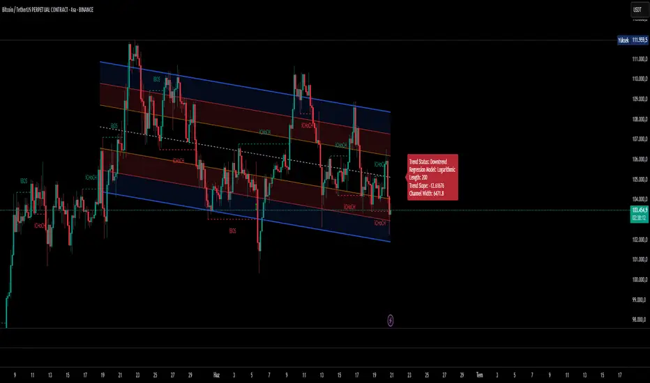
LogTrend Retest EngineLogTrend Retest Engine (LTRE)
LogTrend Retest Engine (LTRE) is an advanced trend-continuation overlay designed to identify high-probability breakout retests using logarithmic regression , volatility-adjusted deviation bands , and market regime filtering .
Unlike traditional channels or moving averages, LTRE models price behavior in log space , allowing it to adapt naturally to exponential market moves common in crypto, indices, and long-term trends.
🔹 How It Works
Logarithmic Regression Core
Performs linear regression on log-transformed price and time
Produces a structurally accurate trend midline that scales with price growth
Volatility-Adjusted Deviation Bands
Dynamic upper and lower zones based on statistical deviation
ATR weighting expands or contracts bands as volatility changes
Adaptive Lookback (Optional)
Automatically adjusts regression length using volatility pressure
Faster response in high-volatility environments, smoother in consolidation
🔹 Market Regime Detection
LTRE actively filters conditions using:
R² trend strength (trend quality, not just slope)
Volatility compression vs expansion
User-defined minimum trend strength threshold
Signals are disabled during ranging or low-quality conditions .
🔹 Breakout → Retest Signal Logic
LTRE does not chase breakouts.
Signals trigger only when:
1. Price breaks cleanly outside the deviation band
2. Market regime is confirmed as trending
3. Price performs a controlled retest within a user-defined tolerance
BUY
Break above upper band → retest → trend confirmed
SELL
Break below lower band → retest → trend confirmed
This structure is designed to reduce false breakouts and late entries.
🔹 Visual & Projection Tools
Clean midline and deviation bands
Optional filled zones
Optional future trend projection for forward structure planning
On-chart statistics for trend strength and volatility compression
🔹 Best Use Cases
Trend continuation & pullback strategies
Crypto, Forex, Indices, and equities
Works best on 15m and higher timeframes
⚠️ Disclaimer
LTRE is a decision-support tool , not a complete trading system. Always use proper risk management and confirm signals with additional structure, volume, or higher-timeframe context.
Built for traders who wait for structure — not noise.

Bollinger Bands Regression Forecast [BigBeluga]🔵 OVERVIEW
The Bollinger Bands Regression Forecast combines volatility envelopes from Bollinger Bands with a linear regression-based projection model .
It visualizes both current and future price zones by extrapolating the Bollinger channel forward in time, giving traders a statistical forecast of probable support and resistance behavior.
🔵 CONCEPTS
Classic Bollinger Bands use a moving average (basis) and standard deviation (deviation) to form dynamic envelopes around price.
This indicator enhances them with linear regression slope detection , allowing it to forecast how the band may expand or contract in the future.
Regression is applied to both the band’s basis and deviation components to predict their trajectory for a user-defined number of Forecast Bars .
The resulting forecast creates a smoothed, funnel-shaped projection that dynamically adapts to volatility.
▲ and ▼ markers highlight potential mean reversion points when price crosses the outer bounds of the bands.
🔵 FEATURES
Forecast Engine : Uses linear regression to project Bollinger Band movement into the future.
Dynamic Channel Width : Adapts standard deviation and slope for realistic volatility modeling.
Auto-Labeled Levels : Displays live upper and lower forecast values for quick reference.
Cross Signals : Marks potential overbought and oversold zones with ▲/▼ signals when price exits the band.
Trend-Adaptive Basis Color : Basis line automatically switches color to represent short-term trend direction.
Customizable Colors and Widths for complete visual control.
🔵 HOW TO USE
Apply the indicator to visualize both current Bollinger structure and its forward projection.
Use ▲/▼ breakout markers to identify short-term reversals or volatility shifts.
When price consistently rides the upper band forecast, the trend is strong and likely continuing.
When regression shows narrowing bands ahead, expect a volatility contraction or consolidation period.
For range traders, outer projected bands can be used as potential mean reversion entry points .
Combine with volume or momentum filters to confirm whether breakouts are genuine or fading.
🔵 CONCLUSION
Bollinger Bands Regression Forecast transforms classic Bollinger analysis into a predictive forecasting model .
By merging volatility dynamics with regression-based extrapolation, it provides traders with a forward-looking visualization of likely price boundaries — revealing not only where volatility is but also where it’s heading next.

Volume Weighted Volatility RegimeThe Volume-Weighted Volatility Regime (VWVR) is a market analysis tool that dissects total volatility to classify the current market 'character' or 'regime'. Using a Linear Regression model, it decomposes volatility into Trend, Residual (mean-reversion), and Within-Bar (noise) components.
Key Features:
Seven-Stage Regime Classification: The indicator's primary output is a regime value from -3 to +3, identifying the market state:
+3 (Strong Bull Trend): High directional, upward volatility.
+2 (Choppy Bull): Moderate upward trend with noise.
+1 (Quiet Bull): Low volatility, slight upward drift.
0 (Neutral): No clear directional bias.
-1 (Quiet Bear): Low volatility, slight downward drift.
-2 (Choppy Bear): Moderate downward trend with noise.
-3 (Strong Bear Trend): High directional, downward volatility.
Advanced Volatility Decomposition: The regime is derived from a three-component volatility model that separates price action into Trend (momentum), Residual (mean-reversion), and Within-Bar (noise) variance. The classification is determined by comparing the 'Trend' ratio against the user-defined 'Trend Threshold' and 'Quiet Threshold'.
Dual-Level Analysis: The indicator analyzes market character on two levels simultaneously:
Inter-Bar Regime (Background Color): Based on the main StdDev Length, showing the overall market character.
Intra-Bar Regime (Column Color): Based on a high-resolution analysis within each single bar ('Intra-Bar Timeframe'), showing the micro-structural character.
Calculation Options:
Statistical Model: The 'Estimate Bar Statistics' option (enabled by default) uses a statistical model ('Estimator') to perform the decomposition. (Assumption: In this mode, the Source input is ignored, and an estimated mean for each bar is used instead).
Normalization: An optional 'Normalize Volatility' setting calculates an Exponential Regression Curve (log-space).
Volume Weighting: An option (Volume weighted) applies volume weighting to all volatility calculations.
Multi-Timeframe (MTF) Capability: The entire dual-level analysis can be run on a higher timeframe (using the Timeframe input), with standard options to handle gaps (Fill Gaps) and prevent repainting (Wait for...).
Integrated Alerts: Includes 22 comprehensive alerts that trigger whenever the 'Inter-Bar Regime' or the 'Intra-Bar Regime' crosses one of the key thresholds (e.g., 'Regime crosses above Neutral Line'), or when the 'Intra-Bar Dominance' crosses the 50% mark.
Caution: Real-Time Data Behavior (Intra-Bar Repainting) This indicator uses high-resolution intra-bar data. As a result, the values on the current, unclosed bar (the real-time bar) will update dynamically as new intra-bar data arrives. This behavior is normal and necessary for this type of analysis. Signals should only be considered final after the main chart bar has closed.
DISCLAIMER
For Informational/Educational Use Only: This indicator is provided for informational and educational purposes only. It does not constitute financial, investment, or trading advice, nor is it a recommendation to buy or sell any asset.
Use at Your Own Risk: All trading decisions you make based on the information or signals generated by this indicator are made solely at your own risk.
No Guarantee of Performance: Past performance is not an indicator of future results. The author makes no guarantee regarding the accuracy of the signals or future profitability.
No Liability: The author shall not be held liable for any financial losses or damages incurred directly or indirectly from the use of this indicator.
Signals Are Not Recommendations: The alerts and visual signals (e.g., crossovers) generated by this tool are not direct recommendations to buy or sell. They are technical observations for your own analysis and consideration.

Volume Weighted Intra Bar LR Standard DeviationThis indicator analyzes market character by providing a detailed view of volatility. It applies a Linear Regression model to intra-bar price action, dissecting the total volatility of each bar into three distinct components.
Key Features:
Three-Component Volatility Decomposition: By analyzing a lower timeframe ('Intra-Bar Timeframe'), the indicator separates each bar's volatility into:
Trend Volatility (Green/Red): Volatility explained by the intra-bar linear regression slope (Momentum).
Residual Volatility (Yellow): Volatility from price oscillating around the intra-bar trendline (Mean-Reversion).
Within-Bar Volatility (Blue): Volatility derived from the range of each intra-bar candle (Noise/Choppiness).
Layered Column Visualization: The indicator plots these components as a layered column chart. The size of each colored layer visually represents the dominance of each volatility character.
Dual Display Modes: The indicator offers two modes to visualize this decomposition:
Absolute Mode: Displays the total standard deviation as the column height, showing the absolute magnitude of volatility and the contribution of each component.
Normalized Mode: Displays the components as a 100% stacked column chart (scaled from 0 to 1), focusing purely on the percentage ratio of Trend, Residual, and Noise.
Calculation Options:
Statistical Model: The 'Estimate Bar Statistics' option (enabled by default) uses a statistical model ('Estimator') to perform the decomposition. (Assumption: In this mode, the Source input is ignored, and an estimated mean for each bar is used instead).
Normalization: An optional 'Normalize Volatility' setting calculates an Exponential Regression Curve (log-space).
Volume Weighting: An option (Volume weighted) applies volume weighting to all intra-bar calculations.
Multi-Component Pivot Detection: Includes a pivot detector that identifies significant turning points (highs and lows) in both the Total Volatility and the Trend Volatility Ratio. (Note: These pivots are only plotted when 'Plot Mode' is set to 'Absolute').
Note on Confirmation (Lag): Pivot signals are confirmed using a lookback method. A pivot is only plotted after the Pivot Right Bars input has passed, which introduces an inherent lag.
Multi-Timeframe (MTF) Capability:
MTF Analysis: The entire intra-bar analysis can be run on a higher timeframe (using the Timeframe input), with standard options to handle gaps (Fill Gaps) and prevent repainting (Wait for...).
Limitation: The Pivot detection (Calculate Pivots) is disabled if a Higher Timeframe (HTF) is selected.
Integrated Alerts: Includes 9 comprehensive alerts for:
Volatility character changes (e.g., 'Character Change from Noise to Trend').
Dominant character emerging (e.g., 'Bullish Trend Character Emerging').
Total Volatility pivot (High/Low) detection.
Trend Volatility pivot (High/Low) detection.
Caution! Real-Time Data Behavior (Intra-Bar Repainting) This indicator uses high-resolution intra-bar data. As a result, the values on the current, unclosed bar (the real-time bar) will update dynamically as new intra-bar data arrives. This behavior is normal and necessary for this type of analysis. Signals should only be considered final after the main chart bar has closed.
DISCLAIMER
For Informational/Educational Use Only: This indicator is provided for informational and educational purposes only. It does not constitute financial, investment, or trading advice, nor is it a recommendation to buy or sell any asset.
Use at Your Own Risk: All trading decisions you make based on the information or signals generated by this indicator are made solely at your own risk.
No Guarantee of Performance: Past performance is not an indicator of future results. The author makes no guarantee regarding the accuracy of the signals or future profitability.
No Liability: The author shall not be held liable for any financial losses or damages incurred directly or indirectly from the use of this indicator.
Signals Are Not Recommendations: The alerts and visual signals (e.g., crossovers) generated by this tool are not direct recommendations to buy or sell. They are technical observations for your own analysis and consideration.

Volume Weighted LR Standard DeviationThis indicator analyzes market character by decomposing total volatility into three distinct, interpretable components based on a Linear Regression model.
Key Features:
Three-Component Volatility Decomposition: The indicator separates volatility based on the 'Estimate Bar Statistics' option.
Standard Mode (Estimate Bar Statistics = OFF): Calculates volatility based on the selected Source (dies führt hauptsächlich zu 'Trend'- und 'Residual'-Volatilität).
Decomposition Mode (Estimate Bar Statistics = ON): The indicator uses a statistical model ('Estimator') to calculate within-bar volatility. (Assumption: In this mode, the Source input is ignored, and an estimated mean for each bar is used instead). This separates volatility into:
Trend Volatility (Green/Red): Volatility explained by the regression's slope (Momentum).
Residual Volatility (Yellow): Volatility from price oscillating around the regression line (Mean-Reversion).
Within-Bar Volatility (Blue): Volatility from the high-low range of each bar (Noise/Choppiness).
Dual Display Modes: The indicator offers two modes to visualize this decomposition:
Absolute Mode: Displays the total standard deviation as a stacked area chart, partitioned by the variance ratio of the three components.
Normalized Mode: Displays the direct variance ratio (proportion) of each component relative to the total (0-1), ideal for identifying the dominant market character.
Calculation Options:
Normalization: An optional 'Normalize Volatility' setting calculates an Exponential Regression Curve (log-space), making the analysis suitable for growth assets.
Volume Weighting: An option (Volume weighted) applies volume weighting to all regression and volatility calculations.
Multi-Component Pivot Detection: Includes a pivot detector that identifies significant turning points (highs and lows) in both the Total Volatility and the Trend Volatility Ratio. (Note: These pivots are only plotted when 'Plot Mode' is set to 'Absolute').
Note on Confirmation (Lag): Pivot signals are confirmed using a lookback method. A pivot is only plotted after the Pivot Right Bars input has passed, which introduces an inherent lag.
Multi-Timeframe (MTF) Capability:
MTF Volatility Lines: The volatility lines can be calculated on a higher timeframe, with standard options to handle gaps (Fill Gaps) and prevent repainting (Wait for...).
Limitation: The Pivot detection (Calculate Pivots) is disabled if a Higher Timeframe (HTF) is selected.
Integrated Alerts: Includes 9 comprehensive alerts for:
Volatility character changes (e.g., 'Character Change from Noise to Trend').
Dominant character emerging (e.g., 'Bullish Trend Character Emerging').
Total Volatility pivot (High/Low) detection.
Trend Volatility pivot (High/Low) detection.
DISCLAIMER
For Informational/Educational Use Only: This indicator is provided for informational and educational purposes only. It does not constitute financial, investment, or trading advice, nor is it a recommendation to buy or sell any asset.
Use at Your Own Risk: All trading decisions you make based on the information or signals generated by this indicator are made solely at your own risk.
No Guarantee of Performance: Past performance is not an indicator of future results. The author makes no guarantee regarding the accuracy of the signals or future profitability.
No Liability: The author shall not be held liable for any financial losses or damages incurred directly or indirectly from the use of this indicator.
Signals Are Not Recommendations: The alerts and visual signals (e.g., crossovers) generated by this tool are not direct recommendations to buy or sell. They are technical observations for your own analysis and consideration.

Volume Weighted Linear Regression BandThe Volume-Weighted Linear Regression Band (VWLRBd) is a volatility channel that uses a Linear Regression line as its dynamic baseline. Its primary feature is the decomposition of total volatility into two distinct components, visualized as layered bands.
Key Features:
Volatility Decomposition: The indicator separates volatility based on the 'Estimate Bar Statistics' option.
Standard Mode (Estimate Bar Statistics = OFF): The indicator functions as a standard (Volume-Weighted) Linear Regression Channel. It plots a single set of bands based on the standard deviation of the residuals (the error between the Source price and the regression line).
Decomposition Mode (Estimate Bar Statistics = ON): The indicator uses a statistical model ('Estimator') to calculate within-bar volatility. (Assumption: In this mode, the Source input is ignored, and an estimated mean for each bar is used for the regression). This mode displays two sets of bands:
Inner Bands: Show only the contribution of the 'residual' (trend noise) volatility, calculated proportionally.
Outer Bands: Show the total volatility (the sum of residual and within-bar components).
Regression Baseline (Linear / Exponential): The central line is a (Volume-Weighted) Linear Regression curve. An optional 'Normalize' mode performs all calculations in logarithmic space, transforming the baseline into an Exponential Regression Curve and the bands into constant percentage deviations, suitable for analyzing growth assets.
Volume Weighting: An option (Volume weighted) allows for volume to be incorporated into the calculation of both the regression baseline and the volatility decomposition, giving more influence to high-participation bars.
Multi-Timeframe (MTF) Engine: The indicator includes an MTF conversion block. When a Higher Timeframe (HTF) is selected, advanced options become available: Fill Gaps handles data gaps, and Wait for timeframe to close prevents repainting by ensuring the indicator only updates when the HTF bar closes.
Integrated Alerts: Includes a full set of built-in alerts for the source price crossing over or under the central regression line and the outermost calculated volatility band.
DISCLAIM_
For Informational/Educational Use Only: This indicator is provided for informational and educational purposes only. It does not constitute financial, investment, or trading advice, nor is it a recommendation to buy or sell any asset.
Use at Your Own Risk: All trading decisions you make based on the information or signals generated by this indicator are made solely at your own risk.
No Guarantee of Performance: Past performance is not an indicator of future results. The author makes no guarantee regarding the accuracy of the signals or future profitability.
No Liability: The author shall not be held liable for any financial losses or damages incurred directly or indirectly from the use of this indicator.
Signals Are Not Recommendations: The alerts and visual signals (e.g., crossovers) generated by this tool are not direct recommendations to buy or sell. They are technical observations for your own analysis and consideration.

Volume Weighted Linear Regression ChannelThis indicator plots a dynamic channel around a Linear Regression trendline. It provides a framework for identifying the prevailing trend and assessing price extremes based on volatility.
Key Features:
Linear Regression Baseline: The channel's centerline is a (Volume-Weighted) Linear Regression line. This line represents the 'best fit' for the recent price action, serving as a responsive baseline for the trend.
Volatility Decomposition: The indicator's primary feature is its ability to decompose volatility, controlled by the 'Estimate Bar Statistics' option.
Standard Mode (Estimate Bar Statistics = OFF): Calculates a standard linear regression channel. The bands represent the standard deviation of the residuals (the error) between the Source price and the regression line.
Decomposition Mode (Estimate Bar Statistics = ON): The indicator uses a statistical model ('Estimator') to calculate within-bar volatility. (Assumption: In this mode, the Source input is ignored, and an estimated mean for each bar is used for the regression). This mode displays two sets of bands:
Inner Bands: Show only the contribution of the 'residual' (trend noise) volatility, calculated proportionally.
Outer Bands: Show the total volatility (the sum of residual and within-bar components).
Volume Weighting: An option (Volume weighted) allows for volume to be incorporated into the calculation of both the linear regression and the volatility decomposition, giving more influence to high-participation bars.
Trend Projection: The calculated channel is plotted as a projection, which can be extended forward (Extend Forward) and backward (Extend Backward) in time to provide a visual guide for potential support and resistance.
Integrated Alerts: Includes a full set of built-in alerts for the Source price crossing over or under the calculated upper band, lower band, and the central regression line.
DISCLAIMER
For Informational/Educational Use Only: This indicator is provided for informational and educational purposes only. It does not constitute financial, investment, or trading advice, nor is it a recommendation to buy or sell any asset.
Use at Your Own Risk: All trading decisions you make based on the information or signals generated by this indicator are made solely at your own risk.
No Guarantee of Performance: Past performance is not an indicator of future results. The author makes no guarantee regarding the accuracy of the signals or future profitability.
No Liability: The author shall not be held liable for any financial losses or damages incurred directly or indirectly from the use of this indicator.
Signals Are Not Recommendations: The alerts and visual signals (e.g., crossovers) generated by this tool are not direct recommendations to buy or sell. They are technical observations for your own analysis and consideration.

LibWghtLibrary "LibWght"
This is a library of mathematical and statistical functions
designed for quantitative analysis in Pine Script. Its core
principle is the integration of a custom weighting series
(e.g., volume) into a wide array of standard technical
analysis calculations.
Key Capabilities:
1. **Universal Weighting:** All exported functions accept a `weight`
parameter. This allows standard calculations (like moving
averages, RSI, and standard deviation) to be influenced by an
external data series, such as volume or tick count.
2. **Weighted Averages and Indicators:** Includes a comprehensive
collection of weighted functions:
- **Moving Averages:** `wSma`, `wEma`, `wWma`, `wRma` (Wilder's),
`wHma` (Hull), and `wLSma` (Least Squares / Linear Regression).
- **Oscillators & Ranges:** `wRsi`, `wAtr` (Average True Range),
`wTr` (True Range), and `wR` (High-Low Range).
3. **Volatility Decomposition:** Provides functions to decompose
total variance into distinct components for market analysis.
- **Two-Way Decomposition (`wTotVar`):** Separates variance into
**between-bar** (directional) and **within-bar** (noise)
components.
- **Three-Way Decomposition (`wLRTotVar`):** Decomposes variance
relative to a linear regression into **Trend** (explained by
the LR slope), **Residual** (mean-reversion around the
LR line), and **Within-Bar** (noise) components.
- **Local Volatility (`wLRLocTotStdDev`):** Measures the total
"noise" (within-bar + residual) around the trend line.
4. **Weighted Statistics and Regression:** Provides a robust
function for Weighted Linear Regression (`wLinReg`) and a
full suite of related statistical measures:
- **Between-Bar Stats:** `wBtwVar`, `wBtwStdDev`, `wBtwStdErr`.
- **Residual Stats:** `wResVar`, `wResStdDev`, `wResStdErr`.
5. **Fallback Mechanism:** All functions are designed for reliability.
If the total weight over the lookback period is zero (e.g., in
a no-volume period), the algorithms automatically fall back to
their unweighted, uniform-weight equivalents (e.g., `wSma`
becomes a standard `ta.sma`), preventing errors and ensuring
continuous calculation.
---
**DISCLAIMER**
This library is provided "AS IS" and for informational and
educational purposes only. It does not constitute financial,
investment, or trading advice.
The author assumes no liability for any errors, inaccuracies,
or omissions in the code. Using this library to build
trading indicators or strategies is entirely at your own risk.
As a developer using this library, you are solely responsible
for the rigorous testing, validation, and performance of any
scripts you create based on these functions. The author shall
not be held liable for any financial losses incurred directly
or indirectly from the use of this library or any scripts
derived from it.
wSma(source, weight, length)
Weighted Simple Moving Average (linear kernel).
Parameters:
source (float) : series float Data to average.
weight (float) : series float Weight series.
length (int) : series int Look-back length ≥ 1.
Returns: series float Linear-kernel weighted mean; falls back to
the arithmetic mean if Σweight = 0.
wEma(source, weight, length)
Weighted EMA (exponential kernel).
Parameters:
source (float) : series float Data to average.
weight (float) : series float Weight series.
length (simple int) : simple int Look-back length ≥ 1.
Returns: series float Exponential-kernel weighted mean; falls
back to classic EMA if Σweight = 0.
wWma(source, weight, length)
Weighted WMA (linear kernel).
Parameters:
source (float) : series float Data to average.
weight (float) : series float Weight series.
length (int) : series int Look-back length ≥ 1.
Returns: series float Linear-kernel weighted mean; falls back to
classic WMA if Σweight = 0.
wRma(source, weight, length)
Weighted RMA (Wilder kernel, α = 1/len).
Parameters:
source (float) : series float Data to average.
weight (float) : series float Weight series.
length (simple int) : simple int Look-back length ≥ 1.
Returns: series float Wilder-kernel weighted mean; falls back to
classic RMA if Σweight = 0.
wHma(source, weight, length)
Weighted HMA (linear kernel).
Parameters:
source (float) : series float Data to average.
weight (float) : series float Weight series.
length (int) : series int Look-back length ≥ 1.
Returns: series float Linear-kernel weighted mean; falls back to
classic HMA if Σweight = 0.
wRsi(source, weight, length)
Weighted Relative Strength Index.
Parameters:
source (float) : series float Price series.
weight (float) : series float Weight series.
length (simple int) : simple int Look-back length ≥ 1.
Returns: series float Weighted RSI; uniform if Σw = 0.
wAtr(tr, weight, length)
Weighted ATR (Average True Range).
Implemented as WRMA on *true range*.
Parameters:
tr (float) : series float True Range series.
weight (float) : series float Weight series.
length (simple int) : simple int Look-back length ≥ 1.
Returns: series float Weighted ATR; uniform weights if Σw = 0.
wTr(tr, weight, length)
Weighted True Range over a window.
Parameters:
tr (float) : series float True Range series.
weight (float) : series float Weight series.
length (int) : series int Look-back length ≥ 1.
Returns: series float Weighted mean of TR; uniform if Σw = 0.
wR(r, weight, length)
Weighted High-Low Range over a window.
Parameters:
r (float) : series float High-Low per bar.
weight (float) : series float Weight series.
length (int) : series int Look-back length ≥ 1.
Returns: series float Weighted mean of range; uniform if Σw = 0.
wBtwVar(source, weight, length, biased)
Weighted Between Variance (biased/unbiased).
Parameters:
source (float) : series float Data series.
weight (float) : series float Weight series.
length (int) : series int Look-back length ≥ 2.
biased (bool) : series bool true → population (biased); false → sample.
Returns:
variance series float The calculated between-bar variance (σ²btw), either biased or unbiased.
sumW series float The sum of weights over the lookback period (Σw).
sumW2 series float The sum of squared weights over the lookback period (Σw²).
wBtwStdDev(source, weight, length, biased)
Weighted Between Standard Deviation.
Parameters:
source (float) : series float Data series.
weight (float) : series float Weight series.
length (int) : series int Look-back length ≥ 2.
biased (bool) : series bool true → population (biased); false → sample.
Returns: series float σbtw uniform if Σw = 0.
wBtwStdErr(source, weight, length, biased)
Weighted Between Standard Error.
Parameters:
source (float) : series float Data series.
weight (float) : series float Weight series.
length (int) : series int Look-back length ≥ 2.
biased (bool) : series bool true → population (biased); false → sample.
Returns: series float √(σ²btw / N_eff) uniform if Σw = 0.
wTotVar(mu, sigma, weight, length, biased)
Weighted Total Variance (= between-group + within-group).
Useful when each bar represents an aggregate with its own
mean* and pre-estimated σ (e.g., second-level ranges inside a
1-minute bar). Assumes the *weight* series applies to both the
group means and their σ estimates.
Parameters:
mu (float) : series float Group means (e.g., HL2 of 1-second bars).
sigma (float) : series float Pre-estimated σ of each group (same basis).
weight (float) : series float Weight series (volume, ticks, …).
length (int) : series int Look-back length ≥ 2.
biased (bool) : series bool true → population (biased); false → sample.
Returns:
varBtw series float The between-bar variance component (σ²btw).
varWtn series float The within-bar variance component (σ²wtn).
sumW series float The sum of weights over the lookback period (Σw).
sumW2 series float The sum of squared weights over the lookback period (Σw²).
wTotStdDev(mu, sigma, weight, length, biased)
Weighted Total Standard Deviation.
Parameters:
mu (float) : series float Group means (e.g., HL2 of 1-second bars).
sigma (float) : series float Pre-estimated σ of each group (same basis).
weight (float) : series float Weight series (volume, ticks, …).
length (int) : series int Look-back length ≥ 2.
biased (bool) : series bool true → population (biased); false → sample.
Returns: series float σtot.
wTotStdErr(mu, sigma, weight, length, biased)
Weighted Total Standard Error.
SE = √( total variance / N_eff ) with the same effective sample
size logic as `wster()`.
Parameters:
mu (float) : series float Group means (e.g., HL2 of 1-second bars).
sigma (float) : series float Pre-estimated σ of each group (same basis).
weight (float) : series float Weight series (volume, ticks, …).
length (int) : series int Look-back length ≥ 2.
biased (bool) : series bool true → population (biased); false → sample.
Returns: series float √(σ²tot / N_eff).
wLinReg(source, weight, length)
Weighted Linear Regression.
Parameters:
source (float) : series float Data series.
weight (float) : series float Weight series.
length (int) : series int Look-back length ≥ 2.
Returns:
mid series float The estimated value of the regression line at the most recent bar.
slope series float The slope of the regression line.
intercept series float The intercept of the regression line.
wResVar(source, weight, midLine, slope, length, biased)
Weighted Residual Variance.
linear regression – optionally biased (population) or
unbiased (sample).
Parameters:
source (float) : series float Data series.
weight (float) : series float Weighting series (volume, etc.).
midLine (float) : series float Regression value at the last bar.
slope (float) : series float Slope per bar.
length (int) : series int Look-back length ≥ 2.
biased (bool) : series bool true → population variance (σ²_P), denominator ≈ N_eff.
false → sample variance (σ²_S), denominator ≈ N_eff - 2.
(Adjusts for 2 degrees of freedom lost to the regression).
Returns:
variance series float The calculated residual variance (σ²res), either biased or unbiased.
sumW series float The sum of weights over the lookback period (Σw).
sumW2 series float The sum of squared weights over the lookback period (Σw²).
wResStdDev(source, weight, midLine, slope, length, biased)
Weighted Residual Standard Deviation.
Parameters:
source (float) : series float Data series.
weight (float) : series float Weight series.
midLine (float) : series float Regression value at the last bar.
slope (float) : series float Slope per bar.
length (int) : series int Look-back length ≥ 2.
biased (bool) : series bool true → population (biased); false → sample.
Returns: series float σres; uniform if Σw = 0.
wResStdErr(source, weight, midLine, slope, length, biased)
Weighted Residual Standard Error.
Parameters:
source (float) : series float Data series.
weight (float) : series float Weight series.
midLine (float) : series float Regression value at the last bar.
slope (float) : series float Slope per bar.
length (int) : series int Look-back length ≥ 2.
biased (bool) : series bool true → population (biased); false → sample.
Returns: series float √(σ²res / N_eff); uniform if Σw = 0.
wLRTotVar(mu, sigma, weight, midLine, slope, length, biased)
Weighted Linear-Regression Total Variance **around the
window’s weighted mean μ**.
σ²_tot = E_w ⟶ *within-group variance*
+ Var_w ⟶ *residual variance*
+ Var_w ⟶ *trend variance*
where each bar i in the look-back window contributes
m_i = *mean* (e.g. 1-sec HL2)
σ_i = *sigma* (pre-estimated intrabar σ)
w_i = *weight* (volume, ticks, …)
ŷ_i = b₀ + b₁·x (value of the weighted LR line)
r_i = m_i − ŷ_i (orthogonal residual)
Parameters:
mu (float) : series float Per-bar mean m_i.
sigma (float) : series float Pre-estimated σ_i of each bar.
weight (float) : series float Weight series w_i (≥ 0).
midLine (float) : series float Regression value at the latest bar (ŷₙ₋₁).
slope (float) : series float Slope b₁ of the regression line.
length (int) : series int Look-back length ≥ 2.
biased (bool) : series bool true → population; false → sample.
Returns:
varRes series float The residual variance component (σ²res).
varWtn series float The within-bar variance component (σ²wtn).
varTrd series float The trend variance component (σ²trd), explained by the linear regression.
sumW series float The sum of weights over the lookback period (Σw).
sumW2 series float The sum of squared weights over the lookback period (Σw²).
wLRTotStdDev(mu, sigma, weight, midLine, slope, length, biased)
Weighted Linear-Regression Total Standard Deviation.
Parameters:
mu (float) : series float Per-bar mean m_i.
sigma (float) : series float Pre-estimated σ_i of each bar.
weight (float) : series float Weight series w_i (≥ 0).
midLine (float) : series float Regression value at the latest bar (ŷₙ₋₁).
slope (float) : series float Slope b₁ of the regression line.
length (int) : series int Look-back length ≥ 2.
biased (bool) : series bool true → population; false → sample.
Returns: series float √(σ²tot).
wLRTotStdErr(mu, sigma, weight, midLine, slope, length, biased)
Weighted Linear-Regression Total Standard Error.
SE = √( σ²_tot / N_eff ) with N_eff = Σw² / Σw² (like in wster()).
Parameters:
mu (float) : series float Per-bar mean m_i.
sigma (float) : series float Pre-estimated σ_i of each bar.
weight (float) : series float Weight series w_i (≥ 0).
midLine (float) : series float Regression value at the latest bar (ŷₙ₋₁).
slope (float) : series float Slope b₁ of the regression line.
length (int) : series int Look-back length ≥ 2.
biased (bool) : series bool true → population; false → sample.
Returns: series float √((σ²res, σ²wtn, σ²trd) / N_eff).
wLRLocTotStdDev(mu, sigma, weight, midLine, slope, length, biased)
Weighted Linear-Regression Local Total Standard Deviation.
Measures the total "noise" (within-bar + residual) around the trend.
Parameters:
mu (float) : series float Per-bar mean m_i.
sigma (float) : series float Pre-estimated σ_i of each bar.
weight (float) : series float Weight series w_i (≥ 0).
midLine (float) : series float Regression value at the latest bar (ŷₙ₋₁).
slope (float) : series float Slope b₁ of the regression line.
length (int) : series int Look-back length ≥ 2.
biased (bool) : series bool true → population; false → sample.
Returns: series float √(σ²wtn + σ²res).
wLRLocTotStdErr(mu, sigma, weight, midLine, slope, length, biased)
Weighted Linear-Regression Local Total Standard Error.
Parameters:
mu (float) : series float Per-bar mean m_i.
sigma (float) : series float Pre-estimated σ_i of each bar.
weight (float) : series float Weight series w_i (≥ 0).
midLine (float) : series float Regression value at the latest bar (ŷₙ₋₁).
slope (float) : series float Slope b₁ of the regression line.
length (int) : series int Look-back length ≥ 2.
biased (bool) : series bool true → population; false → sample.
Returns: series float √((σ²wtn + σ²res) / N_eff).
wLSma(source, weight, length)
Weighted Least Square Moving Average.
Parameters:
source (float) : series float Data series.
weight (float) : series float Weight series.
length (int) : series int Look-back length ≥ 2.
Returns: series float Least square weighted mean. Falls back
to unweighted regression if Σw = 0.

Smooth Theil-SenI wanted to build a Theil-Sen estimator that could run on more than one bar and produce smoother output than the standard implementation. Theil-Sen regression is a non-parametric method that calculates the median slope between all pairs of points in your dataset, which makes it extremely robust to outliers. The problem is that median operations produce discrete jumps, especially when you're working with limited sample sizes. Every time the median shifts from one value to another, you get a step change in your regression line, which creates visual choppiness that can be distracting even though the underlying calculations are sound.
The solution I ended up going with was convolving a Gaussian kernel around the center of the sorted lists to get a more continuous median estimate. Instead of just picking the middle value or averaging the two middle values when you have an even sample size, the Gaussian kernel weights the values near the center more heavily and smoothly tapers off as you move away from the median position. This creates a weighted average that behaves like a median in terms of robustness but produces much smoother transitions as new data points arrive and the sorted list shifts.
There are variance tradeoffs with this approach since you're no longer using the pure median, but they're minimal in practice. The kernel weighting stays concentrated enough around the center that you retain most of the outlier resistance that makes Theil-Sen useful in the first place. What you gain is a regression line that updates smoothly instead of jumping discretely, which makes it easier to spot genuine trend changes versus just the statistical noise of median recalculation. The smoothness is particularly noticeable when you're running the estimator over longer lookback periods where the sorted list is large enough that small kernel adjustments have less impact on the overall center of mass.
The Gaussian kernel itself is a bell curve centered on the median position, with a standard deviation you can tune to control how much smoothing you want. Tighter kernels stay closer to the pure median behavior and give you more discrete steps. Wider kernels spread the weighting further from the center and produce smoother output at the cost of slightly reduced outlier resistance. The default settings strike a balance that keeps the estimator robust while removing most of the visual jitter.
Running Theil-Sen on multiple bars means calculating slopes between all pairs of points across your lookback window, sorting those slopes, and then applying the Gaussian kernel to find the weighted center of that sorted distribution. This is computationally more expensive than simple moving averages or even standard linear regression, but Pine Script handles it well enough for reasonable lookback lengths. The benefit is that you get a trend estimate that doesn't get thrown off by individual spikes or anomalies in your price data, which is valuable when working with noisy instruments or during volatile periods where traditional regression lines can swing wildly.
The implementation maintains sorted arrays for both the slope calculations and the final kernel weighting, which keeps everything organized and makes the Gaussian convolution straightforward. The kernel weights are precalculated based on the distance from the center position, then applied as multipliers to the sorted slope values before summing to get the final smoothed median slope. That slope gets combined with an intercept calculation to produce the regression line values you see plotted on the chart.
What this really demonstrates is that you can take classical statistical methods like Theil-Sen and adapt them with signal processing techniques like kernel convolution to get behavior that's more suited to real-time visualization. The pure mathematical definition of a median is discrete by nature, but financial charts benefit from smooth, continuous lines that make it easier to track changes over time. By introducing the Gaussian kernel weighting, you preserve the core robustness of the median-based approach while gaining the visual smoothness of methods that use weighted averages. Whether that smoothness is worth the minor variance tradeoff depends on your use case, but for most charting applications, the improved readability makes it a good compromise.

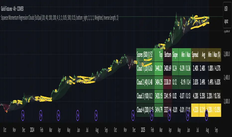
Squeeze Momentum Regression Clouds [SciQua]╭──────────────────────────────────────────────╮
☁️ Squeeze Momentum Regression Clouds
╰──────────────────────────────────────────────╯
🔍 Overview
The Squeeze Momentum Regression Clouds (SMRC) indicator is a powerful visual tool for identifying price compression , trend strength , and slope momentum using multiple layers of linear regression Clouds. Designed to extend the classic squeeze framework, this indicator captures the behavior of price through dynamic slope detection, percentile-based spread analytics, and an optional UI for trend inspection — across up to four customizable regression Clouds .
────────────────────────────────────────────────────────────
╭────────────────╮
⚙️ Core Features
╰────────────────╯
Up to 4 Regression Clouds – Each Cloud is created from a top and bottom linear regression line over a configurable lookback window.
Slope Detection Engine – Identifies whether each band is rising, falling, or flat based on slope-to-ATR thresholds.
Spread Compression Heatmap – Highlights compressed zones using yellow intensity, derived from historical spread analysis.
Composite Trend Scoring – Aggregates directional signals from each Cloud using your chosen weighting model.
Color-Coded Candles – Optional candle coloring reflects the real-time composite score.
UI Table – A toggleable info table shows slopes, compression levels, percentile ranks, and direction scores for each Cloud.
Gradient Cloud Styling – Apply gradient coloring from Cloud 1 to Cloud 4 for visual slope intensity.
Weight Aggregation Options – Use equal weighting, inverse-length weighting, or max pooling across Clouds to determine composite trend strength.
────────────────────────────────────────────────────────────
╭──────────────────────────────────────────╮
🧪 How to Use the Indicator
1. Understand Trend Bias with Cloud Colors
╰──────────────────────────────────────────╯
Each Cloud changes color based on its current slope:
Green indicates a rising trend.
Red indicates a falling trend.
Gray indicates a flat slope — often seen during chop or transitions.
Cloud 1 typically reflects short-term structure, while Cloud 4 represents long-term directional bias. Watch for multi-Cloud alignment — when all Clouds are green or red, the trend is strong. Divergence among Clouds often signals a potential shift.
────────────────────────────────────────────────────────────
╭───────────────────────────────────────────────╮
2. Use Compression Heat to Anticipate Breakouts
╰───────────────────────────────────────────────╯
The space between each Cloud’s top and bottom regression lines is measured, normalized, and analyzed over time. When this spread tightens relative to its history, the script highlights the band with a yellow compression glow .
This visual cue helps identify squeeze zones before volatility expands. If you see compression paired with a changing slope color (e.g., gray to green), this may indicate an impending breakout.
────────────────────────────────────────────────────────────
╭─────────────────────────────────╮
3. Leverage the Optional Table UI
╰─────────────────────────────────╯
The indicator includes a dynamic, floating table that displays real-time metrics per Cloud. These include:
Slope direction and value , with historical Min/Max reference.
Top and Bottom percentile ranks , showing how price sits within the Cloud range.
Current spread width , compared to its historical norms.
Composite score , which blends trend, slope, and compression for that Cloud.
You can customize the table’s position, theme, transparency, and whether to show a combined summary score in the header.
────────────────────────────────────────────────────────────
╭─────────────────────────────────────────────╮
4. Analyze Candle Color for Composite Signals
╰─────────────────────────────────────────────╯
When enabled, the indicator colors candles based on a weighted composite score. This score factors in:
The signed slope of each Cloud (up, down, or flat)
The percentile pressure from the top and bottom bands
The degree of spread compression
Expect green candles in bullish trend phases, red candles during bearish regimes, and gray candles in mixed or low-conviction zones.
Candle coloring provides a visual shorthand for market conditions , useful for intraday scanning or historical backtesting.
────────────────────────────────────────────────────────────
╭────────────────────────╮
🧰 Configuration Guidance
╰────────────────────────╯
To tailor the indicator to your strategy:
Use Cloud lengths like 21, 34, 55, and 89 for a balanced multi-timeframe view.
Adjust the slope threshold (default 0.05) to control how sensitive the trend coloring is.
Set the spread floor (e.g., 0.15) to tune when compression is detected and visualized.
Choose your weighting style : Inverse Length (favor faster bands), Equal, or Max Pooling (most aggressive).
Set composite weights to emphasize trend slope, percentile bias, or compression—depending on your market edge.
────────────────────────────────────────────────────────────
╭────────────────╮
✅ Best Practices
╰────────────────╯
Use aligned Cloud colors across all bands to confirm trend conviction.
Combine slope direction with compression glow for early breakout entry setups.
In choppy markets, watch for Clouds 1 and 2 turning flat while Clouds 3 and 4 remain directional — a sign of potential trend exhaustion or consolidation.
Keep the table enabled during backtesting to manually evaluate how each Cloud behaved during price turns and consolidations.
────────────────────────────────────────────────────────────
╭───────────────────────╮
📌 License & Usage Terms
╰───────────────────────╯
This script is provided under the Creative Commons Attribution-NonCommercial 4.0 International License .
✅ You are allowed to:
Use this script for personal or educational purposes
Study, learn, and adapt it for your own non-commercial strategies
❌ You are not allowed to:
Resell or redistribute the script without permission
Use it inside any paid product or service
Republish without giving clear attribution to the original author
For commercial licensing , private customization, or collaborations, please contact Joshua Danford directly.
Ultimate Regression Channel v5.0 [WhiteStone_Ibrahim]Ultimate Regression Channel v5.0: Comprehensive User Guide
This indicator is designed to visualize the current trend, potential support/resistance levels, and market volatility through a statistical analysis of price action. At its core, it plots a regression line (a trend line) based on prices over a specific period and adds channels based on standard deviation around this line.
1. Core Features and Settings
Length Mode:
Numerical (Manual): You define the number of bars to be used for the regression channel calculation. You can use lower values (e.g., 50-100) for short-term analysis and higher values (e.g., 200-300) to identify long-term trends.
Automatic (Based on Market Structure): This mode automatically draws the channel starting from the highest high or lowest low that has formed within the Auto Scan Period. This allows the indicator to adapt itself to significant market turning points (swing points), which is highly useful.
Regression Model:
Linear: Calculates the trend as a straight line. It generally works well in stable, short-to-medium-term trends.
Logarithmic: Calculates the trend as a curved line. It more accurately reflects price action, especially on long-term charts or for assets that experience exponential growth/decline (like cryptocurrencies or growth stocks).
Channel Widths:
These settings determine how far from the central trend line (in terms of standard deviations) the channels will be drawn.
The 0 (Inner), 1 (Middle), and 2 (Outer) channels represent the "normal" range of price movement and the "extreme" zones. Statistically, about 95% of all price action occurs within the outer channels (2nd standard deviation).
2. Visual Extras and Their Interpretation
Breakout Style:
This feature alerts you when the price closes above the uppermost channel (Channel 2) with a green arrow/background or below the lowermost channel with a red arrow/background.
This is a very important signal. A breakout can signify that the current trend is strengthening and likely to continue (a breakout/trend-following strategy) or that the market has become overextended and may be due for a reversal (an exhaustion/top-bottom signal). It is critical to confirm this signal with other indicators (e.g., RSI, Volume).
Info Label:
This provides an at-a-glance summary of the channel on the right side of the chart:
Trend Status: Identifies the trend as "Uptrend," "Downtrend," or "Sideways" based on the slope of the centerline. The Horizontal Threshold setting allows you to filter out noise by treating very small slopes as "Sideways."
Regression Model and Length: Shows your current settings.
Trend Slope: A numerical value representing how steep or weak the trend is.
Channel Width: Shows the price difference between the outermost channels. This is a measure of current volatility. A widening channel indicates increasing volatility, while a narrowing one indicates decreasing volatility.
3. What Users Should Pay Attention To & Best Practices
Define Your Strategy: Mean Reversion or Breakout?
Mean Reversion: If the market is in a ranging or gently trending phase, the price will tend to revert to the centerline after hitting the outer channels (overbought/oversold zones). In this case, the outer channels can be considered opportunities to sell (upper channel) or buy (lower channel).
Breakout: If a strong trend is in place, a price close beyond an outer channel can be a sign that the trend is accelerating. In this scenario, one might consider taking a position in the direction of the breakout. Correctly analyzing the current market state (ranging vs. trending) is key to deciding which strategy to employ.
Don't Use It in Isolation: No indicator is a holy grail. Use the Regression Channel in conjunction with other tools. Confirm signals with RSI divergences for overbought/oversold conditions, Moving Averages for the overall trend direction, or Volume indicators to confirm the strength of a breakout.
Choose the Right Model: On shorter-term charts (e.g., 1-hour, 4-hour), the Linear model is often sufficient. However, on long-term charts like the daily, weekly, or monthly, the Logarithmic model will provide much more accurate results, especially for assets with parabolic movements.
The Power of Automatic Mode: The Automatic length mode is often the most practical choice because it finds the most logical starting point for you. It saves you the trouble of adjusting settings, especially when analyzing different assets or timeframes.
Use the Alerts: If you don't want to miss the moment the price touches a key channel line, set up an alert from the Alert Settings section for your desired line (e.g., only the "Outer Channels"). This helps you catch opportunities even when you are not in front of the screen.
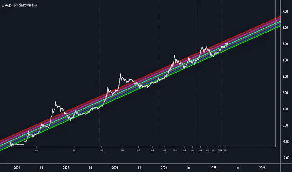
Bitcoin Power Law [LuxAlgo]The Bitcoin Power Law tool is a representation of Bitcoin prices first proposed by Giovanni Santostasi, Ph.D. It plots BTCUSD daily closes on a log10-log10 scale, and fits a linear regression channel to the data.
This channel helps traders visualise when the price is historically in a zone prone to tops or located within a discounted zone subject to future growth.
🔶 USAGE
Giovanni Santostasi, Ph.D. originated the Bitcoin Power-Law Theory; this implementation places it directly on a TradingView chart. The white line shows the daily closing price, while the cyan line is the best-fit regression.
A channel is constructed from the linear fit root mean squared error (RMSE), we can observe how price has repeatedly oscillated between each channel areas through every bull-bear cycle.
Excursions into the upper channel area can be followed by price surges and finishing on a top, whereas price touching the lower channel area coincides with a cycle low.
Users can change the channel areas multipliers, helping capture moves more precisely depending on the intended usage.
This tool only works on the daily BTCUSD chart. Ticker and timeframe must match exactly for the calculations to remain valid.
🔹 Linear Scale
Users can toggle on a linear scale for the time axis, in order to obtain a higher resolution of the price, (this will affect the linear regression channel fit, making it look poorer).
🔶 DETAILS
One of the advantages of the Power Law Theory proposed by Giovanni Santostasi is its ability to explain multiple behaviors of Bitcoin. We describe some key points below.
🔹 Power-Law Overview
A power law has the form y = A·xⁿ , and Bitcoin’s key variables follow this pattern across many orders of magnitude. Empirically, price rises roughly with t⁶, hash-rate with t¹² and the number of active addresses with t³.
When we plot these on log-log axes they appear as straight lines, revealing a scale-invariant system whose behaviour repeats proportionally as it grows.
🔹 Feedback-Loop Dynamics
Growth begins with new users, whose presence pushes the price higher via a Metcalfe-style square-law. A richer price pool funds more mining hardware; the Difficulty Adjustment immediately raises the hash-rate requirement, keeping profit margins razor-thin.
A higher hash rate secures the network, which in turn attracts the next wave of users. Because risk and Difficulty act as braking forces, user adoption advances as a power of three in time rather than an unchecked S-curve. This circular causality repeats without end, producing the familiar boom-and-bust cadence around the long-term power-law channel.
🔹 Scale Invariance & Predictions
Scale invariance means that enlarging the timeline in log-log space leaves the trajectory unchanged.
The same geometric proportions that described the first dollar of value can therefore extend to a projected million-dollar bitcoin, provided no catastrophic break occurs. Institutional ETF inflows supply fresh capital but do not bend the underlying slope; only a persistent deviation from the line would falsify the current model.
🔹 Implications
The theory assigns scarcity no direct role; iterative feedback and the Difficulty Adjustment are sufficient to govern Bitcoin’s expansion. Long-term valuation should focus on position within the power-law channel, while bubbles—sharp departures above trend that later revert—are expected punctuations of an otherwise steady climb.
Beyond about 2040, disruptive technological shifts could alter the parameters, but for the next order of magnitude the present slope remains the simplest, most robust guide.
Bitcoin behaves less like a traditional asset and more like a self-organising digital organism whose value, security, and adoption co-evolve according to immutable power-law rules.
🔶 SETTINGS
🔹 General
Start Calculation: Determine the start date used by the calculation, with any prior prices being ignored. (default - 15 Jul 2010)
Use Linear Scale for X-Axis: Convert the horizontal axis from log(time) to linear calendar time
🔹 Linear Regression
Show Regression Line: Enable/disable the central power-law trend line
Regression Line Color: Choose the colour of the regression line
Mult 1: Toggle line & fill, set multiplier (default +1), pick line colour and area fill colour
Mult 2: Toggle line & fill, set multiplier (default +0.5), pick line colour and area fill colour
Mult 3: Toggle line & fill, set multiplier (default -0.5), pick line colour and area fill colour
Mult 4: Toggle line & fill, set multiplier (default -1), pick line colour and area fill colour
🔹 Style
Price Line Color: Select the colour of the BTC price plot
Auto Color: Automatically choose the best contrast colour for the price line
Price Line Width: Set the thickness of the price line (1 – 5 px)
Show Halvings: Enable/disable dotted vertical lines at each Bitcoin halving
Halvings Color: Choose the colour of the halving lines
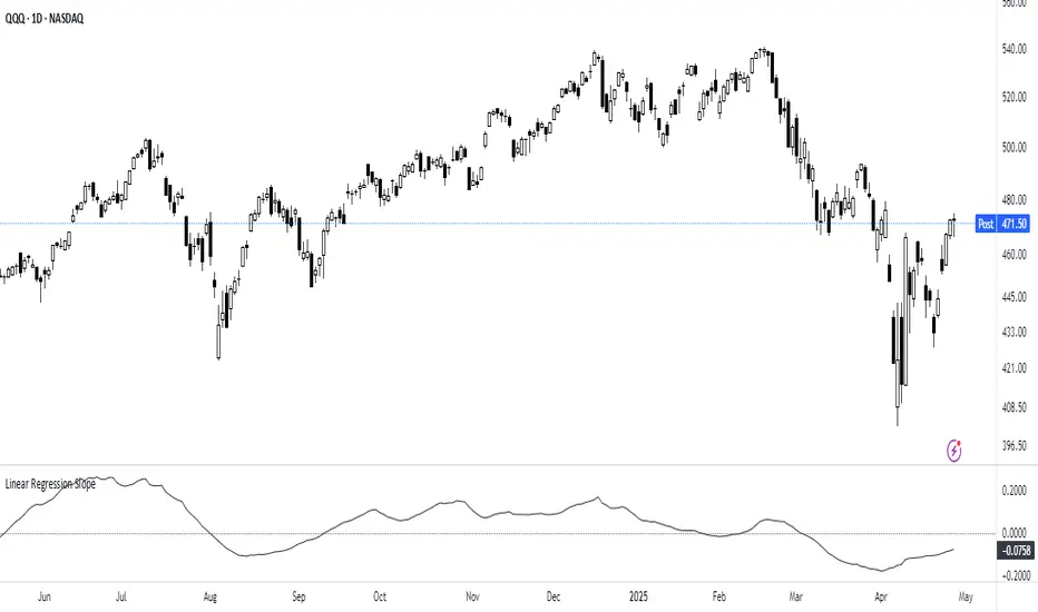
Linear Regression Slope The Linear Regression Slope provides a quantitative measure of trend direction. It fits a linear regression line to the past N closing prices and calculates the slope, representing the average rate of price change per bar.
To ensure comparability across assets and timeframes, the slope is normalized by the ATR over a shorter window. This produces a volatility-adjusted measure which allows for the slope to be interpreted relative to typical price fluctuations.
Mathematically, the slope is derived by minimizing the sum of squared deviations between actual prices and the fitted regression line. A positive normalized slope indicate upwards movement; a negative slope indicate downwards movement. Persistent values near zero could indicate an absence of clear trend, with price dominated by short-term fluctuations or noise.
The definition of a trend depends on the period of observation. The lookback setting should be set based on to the desired timeframe. Shorter lookbacks will respond faster to recent changes but may be more sensitive to noise, while longer lookbacks will emphasize broader structures.
While effective at quantifying existing trends, this method is not predictive. Sudden regime changes, volatility shocks, and non-linear dynamics can all cause rapid slope reversals. Therefore, it is best applied as part of a broader analytical framework.
In summary, the Linear Regression Slope quantifies price direction and serves as a measurable supplement to the visual assessment of trends on price charts.
Additional Features:
Option to display or hide the normalized slope line.
Option to enable background coloring when the slope is above or below zero.
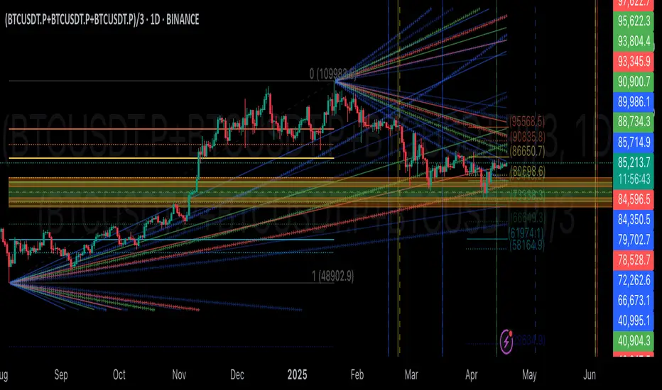
GIGANEVA V6.61 PublicThis enhanced Fibonacci script for TradingView is a powerful, all-in-one tool that calculates Fibonacci Levels, Fans, Time Pivots, and Golden Pivots on both logarithmic and linear scales. Its ability to compute time pivots via fan intersections and Range interactions, combined with user-friendly features like Bool Fib Right, sets it apart. The script maximizes TradingView’s plotting capabilities, making it a unique and versatile tool for technical analysis across various markets.
1. Overview of the Script
The script appears to be a custom technical analysis tool built for TradingView, improving upon an existing script from TradingView’s Community Scripts. It calculates and plots:
Fibonacci Levels: Standard retracement levels (e.g., 0.236, 0.382, 0.5, 0.618, etc.) based on a user-defined price range.
Fibonacci Fans: Trendlines drawn from a high or low point, radiating at Fibonacci ratios to project potential support/resistance zones.
Time Pivots: Points in time where significant price action is expected, determined by the intersection of Fibonacci Fans or their interaction with key price levels.
Golden Pivots: Specific time pivots calculated when the 0.5 Fibonacci Fan (on a logarithmic or linear scale) intersects with its counterpart.
The script supports both logarithmic and linear price scales, ensuring versatility across different charting preferences. It also includes a feature to extend Fibonacci Fans to the right, regardless of whether the user selects the top or bottom of the range first.
2. Key Components Explained
a) Fibonacci Levels and Fans from Top and Bottom of the "Range"
Fibonacci Levels: These are horizontal lines plotted at standard Fibonacci retracement ratios (e.g., 0.236, 0.382, 0.5, 0.618, etc.) based on a user-defined price range (the "Range"). The Range is typically the distance between a significant high (top) and low (bottom) on the chart.
Example: If the high is $100 and the low is $50, the 0.618 retracement level would be at $80.90 ($50 + 0.618 × $50).
Fibonacci Fans: These are diagonal lines drawn from either the top or bottom of the Range, radiating at Fibonacci ratios (e.g., 0.382, 0.5, 0.618). They project potential dynamic support or resistance zones as price evolves over time.
From Top: Fans drawn downward from the high of the Range.
From Bottom: Fans drawn upward from the low of the Range.
Log and Linear Scale:
Logarithmic Scale: Adjusts price intervals to account for percentage changes, which is useful for assets with large price ranges (e.g., cryptocurrencies or stocks with exponential growth). Fibonacci calculations on a log scale ensure ratios are proportional to percentage moves.
Linear Scale: Uses absolute price differences, suitable for assets with smaller, more stable price ranges.
The script’s ability to plot on both scales makes it adaptable to different markets and user preferences.
b) Time Pivots
Time pivots are points in time where significant price action (e.g., reversals, breakouts) is anticipated. The script calculates these in two ways:
Fans Crossing Each Other:
When two Fibonacci Fans (e.g., one from the top and one from the bottom) intersect, their crossing point represents a potential time pivot. This is because the intersection indicates a convergence of dynamic support/resistance zones, increasing the likelihood of a price reaction.
Example: A 0.618 fan from the top crosses a 0.382 fan from the bottom at a specific bar on the chart, marking that bar as a time pivot.
Fans Crossing Top and Bottom of the Range:
A fan line (e.g., 0.5 fan from the bottom) may intersect the top or bottom price level of the Range at a specific time. This intersection highlights a moment where the fan’s projected support/resistance aligns with a key price level, signaling a potential pivot.
Example: The 0.618 fan from the bottom reaches the top of the Range ($100) at bar 50, marking bar 50 as a time pivot.
c) Golden Pivots
Definition: Golden pivots are a special type of time pivot calculated when the 0.5 Fibonacci Fan on one scale (logarithmic or linear) intersects with the 0.5 fan on the opposite scale (or vice versa).
Significance: The 0.5 level is the midpoint of the Fibonacci sequence and often acts as a critical balance point in price action. When fans at this level cross, it suggests a high-probability moment for a price reversal or significant move.
Example: If the 0.5 fan on a logarithmic scale (drawn from the bottom) crosses the 0.5 fan on a linear scale (drawn from the top) at bar 100, this intersection is labeled a "Golden Pivot" due to its confluence of key Fibonacci levels.
d) Bool Fib Right
This is a user-configurable setting (a boolean input in the script) that extends Fibonacci Fans to the right side of the chart.
Functionality: When enabled, the fans project forward in time, regardless of whether the user selected the top or bottom of the Range first. This ensures consistency in visualization, as the direction of the Range selection (top-to-bottom or bottom-to-top) does not affect the fan’s extension.
Use Case: Traders can use this to project future support/resistance zones without worrying about how they defined the Range, improving usability.
3. Why Is This Code Unique?
Original calculation of Log levels were taken from zekicanozkanli code. Thank you for giving me great Foundation, later modified and applied to Fib fans. The script’s uniqueness stems from its comprehensive integration of Fibonacci-based tools and its optimization for TradingView’s plotting capabilities. Here’s a detailed breakdown:
All-in-One Fibonacci Tool:
Most Fibonacci scripts on TradingView focus on either retracement levels, extensions, or fans.
This script combines:
Fibonacci Levels: Static horizontal lines for retracement and extension.
Fibonacci Fans: Dynamic trendlines for projecting support/resistance.
Time Pivots: Temporal analysis based on fan intersections and Range interactions.
Golden Pivots: Specialized pivots based on 0.5 fan confluences.
By integrating these functions, the script provides a holistic Fibonacci analysis tool, reducing the need for multiple scripts.
Log and Linear Scale Support:
Many Fibonacci tools are designed for linear scales only, which can distort projections for assets with exponential price movements. By supporting both logarithmic and linear scales, the script caters to a wider range of markets (e.g., stocks, forex, crypto) and user preferences.
Time Pivot Calculations:
Calculating time pivots based on fan intersections and Range interactions is a novel feature. Most TradingView scripts focus on price-based Fibonacci levels, not temporal analysis. This adds a predictive element, helping traders anticipate when significant price action might occur.
Golden Pivot Innovation:
The concept of "Golden Pivots" (0.5 fan intersections across scales) is a unique addition. It leverages the symmetry of the 0.5 level and the differences between log and linear scales to identify high-probability pivot points.
Maximized Plot Capabilities:
TradingView imposes limits on the number of plots (lines, labels, etc.) a script can render. This script is coded to fully utilize these limits, ensuring that all Fibonacci levels, fans, pivots, and labels are plotted without exceeding TradingView’s constraints.
This optimization likely involves efficient use of arrays, loops, and conditional plotting to manage resources while delivering a rich visual output.
User-Friendly Features:
The Bool Fib Right option simplifies fan projection, making the tool intuitive even for users who may not consistently select the Range in the same order.
The script’s flexibility in handling top/bottom Range selection enhances usability.
4. Potential Use Cases
Trend Analysis: Traders can use Fibonacci Fans to identify dynamic support/resistance zones in trending markets.
Reversal Trading: Time pivots and Golden Pivots help pinpoint moments for potential price reversals.
Range Trading: Fibonacci Levels provide key price zones for trading within a defined range.
Cross-Market Application: Log/linear scale support makes the script suitable for stocks, forex, commodities, and cryptocurrencies.
The original code was from zekicanozkanli . Thank you for giving me great Foundation.
TASC 2025.05 Trading The Channel█ OVERVIEW
This script implements channel-based trading strategies based on the concepts explained by Perry J. Kaufman in the article "A Test Of Three Approaches: Trading The Channel" from the May 2025 edition of TASC's Traders' Tips . The script explores three distinct trading methods for equities and futures using information from a linear regression channel. Each rule set corresponds to different market behaviors, offering flexibility for trend-following, breakout, and mean-reversion trading styles.
█ CONCEPTS
Linear regression
Linear regression is a model that estimates the relationship between a dependent variable and one or more independent variables by fitting a straight line to the observed data. In the context of financial time series, traders often use linear regression to estimate trends in price movements over time.
The slope of the linear regression line indicates the strength and direction of the price trend. For example, a larger positive slope indicates a stronger upward trend, and a larger negative slope indicates the opposite. Traders can look for shifts in the direction of a linear regression slope to identify potential trend trading signals, and they can analyze the magnitude of the slope to support trading decisions.
One caveat to linear regression is that most financial time series data does not follow a straight line, meaning a regression line cannot perfectly describe the relationships between values. Prices typically fluctuate around a regression line to some degree. As such, analysts often project ranges above and below regression lines, creating channels to model the expected extent of the data's variability. This strategy constructs a channel based on the method used in Kaufman's article. It measures the maximum distances from points on the linear regression line to historical price values, then adds those distances and the current slope to the regression points.
Depending on the trading style, traders might look for prices to move outside an established channel for breakout signals, or they might look for price action to reach extremes within the channel for potential mean reversion opportunities.
█ STRATEGY CALCULATIONS
Primary trade rules
This strategy implements three distinct sets of rules for trend, breakout, and mean-reversion trades based on the methods Kaufman describes in his article:
Trade the trend (Rule 1) : Open new positions when the sign of the slope changes, indicating a potential trend reversal. Close short trades and enter a long trade when the slope changes from negative to positive, and do the opposite when the slope changes from positive to negative.
Trade channel breakouts (Rule 2) : Open new positions when prices cross outside the linear regression channel for the current sample. Close short trades and enter a long trade when the price moves above the channel, and do the opposite when the price moves below the channel.
Trade within the channel (Rule 3) : Open new positions based on price values within the channel's range. Close short trades and enter a long trade when the price is near the channel's low, within a specified percentage of the channel's range, and do the opposite when the price is near the channel's high. With this rule, users can also filter the trades based on the channel's slope. When the filter is active, long positions are allowed only when the slope is positive, and short positions are allowed only when it is negative.
Position sizing
Kaufman's strategy uses specific trade sizes for equities and futures markets:
For an equities symbol, the number of shares traded is $10,000 divided by the current price.
For a futures symbol, the number of contracts traded is based on a volatility-adjusted formula that divides $25,000 by the product of the 20-bar average true range and the instrument's point value.
By default, this script automatically uses these sizes for its trade simulation on equities and futures symbols and does not simulate trading on other symbols. However, users can control position sizes from the "Settings/Properties" tab and enable trade simulation on other symbol types by selecting the "Manual" option in the script's "Position sizing" input.
Stop-loss
This strategy includes the option to place an accompanying stop-loss order for each trade, which users can enable from the "SL %" input in the "Settings/Inputs" tab. When enabled, the strategy places a stop-loss order at a specified percentage distance from the closing price where the entry order occurs, allowing users to compare how the strategy performs with added loss protection.
█ USAGE
This strategy adapts its display logic for the three trading approaches based on the rule selected in the "Trade rule" input:
For all rules, the script plots the linear regression slope in a separate pane. The plot is color-coded to indicate whether the current slope is positive or negative.
When the selected rule is "Trade the trend", the script plots triangles in the separate pane to indicate when the slope's direction changes from positive to negative or vice versa. Additionally, it plots a color-coded SMA on the main chart pane, allowing visual comparison of the slope to directional changes in a moving average.
When the rule is "Trade channel breakouts" or "Trade within the channel", the script draws the current period's linear regression channel on the main chart pane, and it plots bands representing the history of the channel values from the specified start time onward.
When the rule is "Trade within the channel", the script plots overbought and oversold zones between the bands based on a user-specified percentage of the channel range to indicate the value ranges where new trades are allowed.
Users can customize the strategy's calculations with the following additional inputs in the "Settings/Inputs" tab:
Start date : Sets the date and time when the strategy begins simulating trades. The script marks the specified point on the chart with a gray vertical line. The plots for rules 2 and 3 display the bands and trading zones from this point onward.
Period : Specifies the number of bars in the linear regression channel calculation. The default is 40.
Linreg source : Specifies the source series from which to calculate the linear regression values. The default is "close".
Range source : Specifies whether the script uses the distances from the linear regression line to closing prices or high and low prices to determine the channel's upper and lower ranges for rules 2 and 3. The default is "close".
Zone % : The percentage of the channel's overall range to use for trading zones with rule 3. The default is 20, meaning the width of the upper and lower zones is 20% of the range.
SL% : If the checkbox is selected, the strategy adds a stop-loss to each trade at the specified percentage distance away from the closing price where the entry order occurs. The checkbox is deselected by default, and the default percentage value is 5.
Position sizing : Determines whether the strategy uses Kaufman's predefined trade sizes ("Auto") or allows user-defined sizes from the "Settings/Properties" tab ("Manual"). The default is "Auto".
Long trades only : If selected, the strategy does not allow short positions. It is deselected by default.
Trend filter : If selected, the strategy filters positions for rule 3 based on the linear regression slope, allowing long positions only when the slope is positive and short positions only when the slope is negative. It is deselected by default.
NOTE: Because of this strategy's trading rules, the simulated results for a specific symbol or channel configuration might have significantly fewer than 100 trades. For meaningful results, we recommend adjusting the start date and other parameters to achieve a reasonable number of closed trades for analysis.
Additionally, this strategy does not specify commission and slippage amounts by default, because these values can vary across market types. Therefore, we recommend setting realistic values for these properties in the "Cost simulation" section of the "Settings/Properties" tab.

TrendLibrary "Trend"
calculateSlopeTrend(source, length, thresholdMultiplier)
Parameters:
source (float)
length (int)
thresholdMultiplier (float)
Purpose:
The primary goal of this function is to determine the short-term trend direction of a given data series (like closing prices). It does this by calculating the slope of the data over a specified period and then comparing that slope against a dynamic threshold based on the data's recent volatility. It classifies the trend into one of three states: Upward, Downward, or Flat.
Parameters:
`source` (Type: `series float`): This is the input data series you want to analyze. It expects a series of floating-point numbers, typically price data like `close`, `open`, `hl2` (high+low)/2, etc.
`length` (Type: `int`): This integer defines the lookback period. The function will analyze the `source` data over the last `length` bars to calculate the slope and standard deviation.
`thresholdMultiplier` (Type: `float`, Default: `0.1`): This is a sensitivity factor. It's multiplied by the standard deviation to determine how steep the slope needs to be before it's considered a true upward or downward trend. A smaller value makes it more sensitive (detects trends earlier, potentially more false signals), while a larger value makes it less sensitive (requires a stronger move to confirm a trend).
Calculation Steps:
Linear Regression: It first calculates the value of a linear regression line fitted to the `source` data over the specified `length` (`ta.linreg(source, length, 0)`). Linear regression finds the "best fit" straight line through the data points.
Slope Calculation: It then determines the slope of this linear regression line. Since `ta.linreg` gives the *value* of the line on the current bar, the slope is calculated as the difference between the current bar's linear regression value (`linRegValue`) and the previous bar's value (`linRegValue `). A positive difference means an upward slope, negative means downward.
Volatility Measurement: It calculates the standard deviation (`ta.stdev(source, length)`) of the `source` data over the same `length`. Standard deviation is a measure of how spread out the data is, essentially quantifying its recent volatility.
Adaptive Threshold: An adaptive threshold (`threshold`) is calculated by multiplying the standard deviation (`stdDev`) by the `thresholdMultiplier`. This is crucial because it means the definition of a "flat" trend adapts to the market's volatility. In volatile times, the threshold will be wider, requiring a larger slope to signal a trend. In quiet times, the threshold will be narrower.
Trend Determination: Finally, it compares the calculated `slope` to the adaptive `threshold`:
If the `slope` is greater than the positive `threshold`, the trend is considered **Upward**, and the function returns `1`.
If the `slope` is less than the negative `threshold` (`-threshold`), the trend is considered **Downward**, and the function returns `-1`.
If the `slope` falls between `-threshold` and `+threshold` (inclusive of 0), the trend is considered **Flat**, and the function returns `0`.
Return Value:
The function returns an integer representing the determined trend direction:
`1`: Upward trend
`-1`: Downward trend
`0`: Flat trend
In essence, this library function provides a way to gauge trend direction using linear regression, but with a smart filter (the adaptive threshold) to avoid classifying minor noise or low-volatility periods as significant trends.
Linear Regression Volume Profile [ChartPrime]LR VolumeProfile
This indicator combines a Linear Regression channel with a dynamic volume profile, giving traders a powerful way to visualize both directional price movement and volume concentration along the trend.
⯁ KEY FEATURES
Linear Regression Channel: Draws a statistically fitted channel to track the market trend over a defined period.
Volume Profile Overlay: Splits the channel into multiple horizontal levels and calculates volume traded within each level.
Percentage-Based Labels: Displays each level's share of total volume as a percentage, offering a clean way to see high and low volume zones.
Gradient Bars: Profile bars are colored using a gradient scale from yellow (low volume) to red (high volume), making it easy to identify key interest areas.
Adjustable Profile Width and Resolution: Users can change the width of profile bars and spacing between levels.
Channel Direction Indicator: An arrow inside a floating label shows the direction (up or down) of the current linear regression slope.
Level Style Customization: Choose from solid, dashed, or dotted lines for visual preference.
⯁ HOW TO USE
Use the Linear Regression channel to determine the dominant price trend direction.
Analyze the volume bars to spot key levels where the majority of volume was traded—these act as potential support/resistance zones.
Pay attention to the largest profile bars—these often mark zones of institutional interest or price consolidation.
The arrow label helps quickly assess whether the trend is upward or downward.
Combine this tool with price action or momentum indicators to build high-confidence trading setups.
⯁ CONCLUSION
LR Volume Profile is a precision tool for traders who want to merge trend analysis with volume insight. By integrating linear regression trendlines with a clean and readable volume distribution, this indicator helps traders find price levels that matter the most—backed by volume, trend, and structure. Whether you're spotting high-volume nodes or gauging directional flow, this toolkit elevates your decision-making process with clarity and depth.
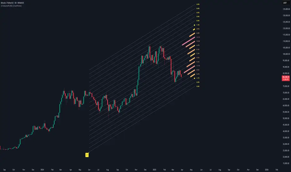
Multi-Anchored Linear Regression Channels [TANHEF]█ Overview:
The 'Multi-Anchored Linear Regression Channels ' plots multiple dynamic regression channels (or bands) with unique selectable calculation types for both regression and deviation. It leverages a variety of techniques, customizable anchor sources to determine regression lengths, and user-defined criteria to highlight potential opportunities.
Before getting started, it's worth exploring all sections, but make sure to review the Setup & Configuration section in particular. It covers key parameters like anchor type, regression length, bias, and signal criteria—essential for aligning the tool with your trading strategy.
█ Key Features:
⯁ Multi-Regression Capability:
Plot up to three distinct regression channels and/or bands simultaneously, each with customizable anchor types to define their length.
⯁ Regression & Deviation Methods:
Regressions Types:
Standard: Uses ordinary least squares to compute a simple linear trend by averaging the data and deriving a slope and endpoints over the lookback period.
Ridge: Introduces L2 regularization to stabilize the slope by penalizing large coefficients, which helps mitigate multicollinearity in the data.
Lasso: Uses L1 regularization through soft-thresholding to shrink less important coefficients, yielding a simpler model that highlights key trends.
Elastic Net: Combines L1 and L2 penalties to balance coefficient shrinkage and selection, producing a robust weighted slope that handles redundant predictors.
Huber: Implements the Huber loss with iteratively reweighted least squares (IRLS) and EMA-style weights to reduce the impact of outliers while estimating the slope.
Least Absolute Deviations (LAD): Reduces absolute errors using iteratively reweighted least squares (IRLS), yielding a slope less sensitive to outliers than squared-error methods.
Bayesian Linear: Merges prior beliefs with weighted data through Bayesian updating, balancing the prior slope with data evidence to derive a probabilistic trend.
Deviation Types:
Regressive Linear (Reverse): In reverse order (recent to oldest), compute weighted squared differences between the data and a line defined by a starting value and slope.
Progressive Linear (Forward): In forward order (oldest to recent), compute weighted squared differences between the data and a line defined by a starting value and slope.
Balanced Linear: In forward order (oldest to newest), compute regression, then pair to source data in reverse order (newest to oldest) to compute weighted squared differences.
Mean Absolute: Compute weighted absolute differences between each data point and its regression line value, then aggregate them to yield an average deviation.
Median Absolute: Determine the weighted median of the absolute differences between each data point and its regression line value to capture the central tendency of deviations.
Percent: Compute deviation as a percentage of a base value by multiplying that base by the specified percentage, yielding symmetric positive and negative deviations.
Fitted: Compare a regression line with high and low series values by computing weighted differences to determine the maximum upward and downward deviations.
Average True Range: Iteratively compute the weighted average of absolute differences between the data and its regression line to yield an ATR-style deviation measure.
Bias:
Bias: Applies EMA or inverse-EMA style weighting to both Regression and/or Deviation, emphasizing either recent or older data.
⯁ Customizable Regression Length via Anchors:
Anchor Types:
Fixed: Length.
Bar-Based: Bar Highest/Lowest, Volume Highest/Lowest, Spread Highest/Lowest.
Correlation: R Zero, R Highest, R Lowest, R Absolute.
Slope: Slope Zero, Slope Highest, Slope Lowest, Slope Absolute.
Indicator-Based: Indicators Highest/Lowest (ADX, ATR, BBW, CCI, MACD, RSI, Stoch).
Time-Based: Time (Day, Week, Month, Quarter, Year, Decade, Custom).
Session-Based: Session (Tokyo, London, New York, Sydney, Custom).
Event-Based: Earnings, Dividends, Splits.
External: Input Source Highest/Lowest.
Length Selection:
Maximum: The highest allowed regression length (also fixed value of “Length” anchor).
Minimum: The shortest allowed length, ensuring enough bars for a valid regression.
Step: The sampling interval (e.g., 1 checks every bar, 2 checks every other bar, etc.). Increasing the step reduces the loading time, most applicable to “Slope” and “R” anchors.
Adaptive lookback:
Adaptive Lookback: Enable to display regression regardless of too few historical bars.
⯁ Selecting Bias:
Bias applies separately to regression and deviation.
Positive values emphasize recent data (EMA-style), negative invert, and near-zero maintains balance. (e.g., a length 100, bias +1 gives the newest price ~7× more weight than the oldest).
It's best to apply bias to both (regression and deviation) or just the deviation. Biasing only regression may distort deviation visually, while biasing both keeps their relationship intuitive. Using bias only for deviation scales it without altering regression, offering unique analysis.
⯁ Scale Awareness:
Supports linear and logarithmic price scaling, the regression and deviations adjust accordingly.
⯁ Signal Generation & Alerts:
Customizable entry/exit signals and alerts, detailed in the dedicated section below.
⯁ Visual Enhancements & Real-World Examples:
Optional on-chart table display summarizing regression input criteria (display type, anchor type, source, regression type, regression bias, deviation type, deviation bias, deviation multiplier) and key calculated metrics (regression length, slope, Pearson’s R, percentage position within deviations, etc.) for quick reference.
█ Understanding R (Pearson Correlation Coefficient):
Pearson’s R gauges data alignment to a straight-line trend within the regression length:
Range: R varies between –1 and +1.
R = +1 → Perfect positive correlation (strong uptrend).
R = 0 → No linear relationship detected.
R = –1 → Perfect negative correlation (strong downtrend).
This script uses Pearson’s R as an anchor, adjusting regression length to target specific R traits. Strong R (±1) follows the regression channel, while weak R (0) shows inconsistency.
█ Understanding the Slope:
The slope is the direction and rate at which the regression line rises or falls per bar:
Positive Slope (>0): Uptrend – Steeper means faster increase.
Negative Slope (<0): Downtrend – Steeper means sharper drop.
Zero or Near-Zero Slope: Sideways – Indicating range-bound conditions.
This script uses highest and lowest slope as an anchor, where extremes highlight strong moves and trend lines, while values near zero indicate sideways action and possible support/resistance.
█ Setup & Configuration:
Whether you’re new to this script or want to quickly adjust all critical parameters, the panel below shows the main settings available. You can customize everything from the anchor type and maximum length to the bias, signal conditions, and more.
Scale (select Log Scale for logarithmic, otherwise linear scale).
Display (regression channel and/or bands).
Anchor (how regression length is determined).
Length (control bars analyzed):
• Max – Upper limit.
• Min – Prevents regression from becoming too short.
• Step – Controls scanning precision; increasing Step reduces load time.
Regression:
• Type – Calculation method.
• Bias – EMA-style emphasis (>0=new bars weighted more; <0=old bars weighted more).
Deviation:
• Type – Calculation method.
• Bias – EMA-style emphasis (>0=new bars weighted more; <0=old bars weighted more).
• Multiplier - Adjusts Upper and Lower Deviation.
Signal Criteria:
• % (Price vs Deviation) – (0% = lower deviation, 50% = regression, 100% = upper deviation).
• R – (0 = no correlation, ±1 = perfect correlation; >0 = +slope, <0 = -slope).
Table (analyze table of input settings, calculated results, and signal criteria).
Adaptive Lookback (display regression while too few historical bars).
Multiple Regressions (steps 2 to 7 apply to #1, #2, and #3 regressions).
█ Signal Generation & Alerts:
The script offers customizable entry and exit signals with flexible criteria and visual cues (background color, dots, or triangles). Alerts can also be triggered for these opportunities.
Percent Direction Criteria:
(0% = lower deviation, 50% = regression line, 100% = upper deviation)
Above %: Triggers if price is above a specified percent of the deviation channel.
Below %: Triggers if price is below a specified percent of the deviation channel.
(Blank): Ignores the percent‐based condition.
Pearson's R (Correlation) Direction Criteria:
(0 = no correlation, ±1 = perfect correlation; >0 = positive slope, <0 = negative slope)
Above R / Below R: Compares the correlation to a threshold.
Above│R│ / Below│R│: Uses absolute correlation to focus on strength, ignoring direction.
Zero to R: Checks if R is in the 0-to-threshold range.
(Blank): Ignores correlation-based conditions.
█ User Tips & Best Practices:
Choose an anchor type that suits your strategy, “Bar Highest/Lowest” automatically spots commonly used regression zones, while “│R│ Highest” targets strong linear trends.
Consider enabling or disabling the Adaptive Lookback feature to ensure you always have a plotted regression if your chart doesn’t meet the maximum-length requirement.
Use a small Step size (1) unless relying on R-correlation or slope-based anchors as the are time-consuming to calculate. Larger steps speed up calculations but reduce precision.
Fine-tune settings such as lookback periods, regression bias, and deviation multipliers, or trend strength. Small adjustments can significantly affect how channels and signals behave.
To reduce loading time , show only channels (not bands) and disable signals, this limits calculations to the last bar and supports more extreme criteria.
Use the table display to monitor anchor type, calculated length, slope, R value, and percent location at a glance—especially if you have multiple regressions visible simultaneously.
█ Conclusion:
With its blend of advanced regression techniques, flexible deviation options, and a wide range of anchor types, this indicator offers a highly adaptable linear regression channeling system. Whether you're anchoring to time, price extremes, correlation, slope, or external events, the tool can be shaped to fit a variety of strategies. Combined with customizable signals and alerts, it may help highlight areas of confluence and support a more structured approach to identifying potential opportunities.

LinearRegressionLibrary "LinearRegression"
Calculates a variety of linear regression and deviation types, with optional emphasis weighting. Additionally, multiple of slope and Pearson’s R calculations.
calcSlope(_src, _len, _condition)
Calculates the slope of a linear regression over the specified length.
Parameters:
_src (float) : (float) The source data.
_len (int) : (int) The length of the lookback period for the linear regression.
_condition (bool) : (bool) Flag to enable calculation. Set to true to calculate on every bar; otherwise, set to barstate.islast for efficiency.
Returns: (float) The slope of the linear regression.
calcReg(_src, _len, _condition)
Calculates a basic linear regression, returning y1, y2, slope, and average.
Parameters:
_src (float) : (float) The source data series.
_len (int) : (int) The length of the lookback period.
_condition (bool) : (bool) Flag to enable calculation (true = calculate).
Returns: (float ) An array of 4 values: .
calcRegStandard(_src, _len, _emphasis, _condition)
Calculates an Standard linear regression with optional emphasis.
Parameters:
_src (float) : (series float) The source data series.
_len (int) : (int) The length of the lookback period.
_emphasis (float) : (float) The emphasis factor: 0 for equal weight; >0 emphasizes recent bars; <0 emphasizes older bars.
_condition (bool) : (bool) Flag to enable calculation (true = calculate).
Returns: (float ) .
calcRegRidge(_src, _len, lambda, _emphasis, _condition)
Calculates a ridge regression with optional emphasis.
Parameters:
_src (float) : (float) The source data series.
_len (int) : (int) The length of the lookback period.
lambda (float) : (float) The ridge regularization parameter.
_emphasis (float) : (float) The emphasis factor: 0 for equal weight; >0 emphasizes recent bars; <0 emphasizes older bars.
_condition (bool) : (bool) Flag to enable calculation (true = calculate).
Returns: (float ) .
calcRegLasso(_src, _len, lambda, _emphasis, _condition)
Calculates a Lasso regression with optional emphasis.
Parameters:
_src (float) : (float) The source data series.
_len (int) : (int) The length of the lookback period.
lambda (float) : (float) The Lasso regularization parameter.
_emphasis (float) : (float) The emphasis factor: 0 for equal weight; >0 emphasizes recent bars; <0 emphasizes older bars.
_condition (bool) : (bool) Flag to enable calculation (true = calculate).
Returns: (float ) .
calcElasticNetLinReg(_src, _len, lambda1, lambda2, _emphasis, _condition)
Calculates an Elastic Net regression with optional emphasis.
Parameters:
_src (float) : (float) The source data series.
_len (int) : (int) The length of the lookback period.
lambda1 (float) : (float) L1 regularization parameter (Lasso).
lambda2 (float) : (float) L2 regularization parameter (Ridge).
_emphasis (float) : (float) Emphasis factor: 0 for equal weight; >0 emphasizes recent bars; <0 emphasizes older bars.
_condition (bool) : (bool) Flag to enable calculation (true = calculate).
Returns: (float ) .
calcRegHuber(_src, _len, delta, iterations, _emphasis, _condition)
Calculates a Huber regression using Iteratively Reweighted Least Squares (IRLS).
Parameters:
_src (float) : (float) The source data series.
_len (int) : (int) The length of the lookback period.
delta (float) : (float) Huber threshold parameter.
iterations (int) : (int) Number of IRLS iterations.
_emphasis (float) : (float) Emphasis factor: 0 for equal weight; >0 emphasizes recent bars; <0 emphasizes older bars.
_condition (bool) : (bool) Flag to enable calculation (true = calculate).
Returns: (float ) .
calcRegLAD(_src, _len, iterations, _emphasis, _condition)
Calculates a Least Absolute Deviations (LAD) regression via IRLS.
Parameters:
_src (float) : (float) The source data series.
_len (int) : (int) The length of the lookback period.
iterations (int) : (int) Number of IRLS iterations for LAD.
_emphasis (float) : (float) Emphasis factor: 0 for equal weight; >0 emphasizes recent bars; <0 emphasizes older bars.
_condition (bool) : (bool) Flag to enable calculation (true = calculate).
Returns: (float ) .
calcRegBayesian(_src, _len, priorMean, priorSpan, sigma, _emphasis, _condition)
Calculates a Bayesian linear regression with optional emphasis.
Parameters:
_src (float) : (float) The source data series.
_len (int) : (int) The length of the lookback period.
priorMean (float) : (float) The prior mean for the slope.
priorSpan (float) : (float) The prior variance (or span) for the slope.
sigma (float) : (float) The assumed standard deviation of residuals.
_emphasis (float) : (float) Emphasis factor: 0 for equal weight; >0 emphasizes recent bars; <0 emphasizes older bars.
_condition (bool) : (bool) Flag to enable calculation (true = calculate).
Returns: (float ) .
calcRFromLinReg(_src, _len, _slope, _average, _y1, _condition)
Calculates the Pearson correlation coefficient (R) based on linear regression parameters.
Parameters:
_src (float) : (float) The source data.
_len (int) : (int) The length of the lookback period.
_slope (float) : (float) The slope of the linear regression.
_average (float) : (float) The average value of the source data series.
_y1 (float) : (float) The starting point (y-intercept of the oldest bar) for the linear regression.
_condition (bool) : (bool) Flag to enable calculation. Set to true to calculate on every bar; otherwise, set to barstate.islast for efficiency.
Returns: (float) The Pearson correlation coefficient (R) adjusted for the direction of the slope.
calcRFromSource(_src, _len, _condition)
Calculates the correlation coefficient (R) using a specified length and source data.
Parameters:
_src (float) : (float) The source data.
_len (int) : (int) The length of the lookback period.
_condition (bool) : (bool) Flag to enable calculation. Set to true to calculate on every bar; otherwise, set to barstate.islast for efficiency.
Returns: (float) The correlation coefficient (R).
calcSlopeLengthZero(_src, _len, _minLen, _step, _condition)
Identifies the length at which the slope is flattest (closest to zero).
Parameters:
_src (float) : (float) The source data.
_len (int) : (int) The maximum lookback length to consider (minimum of 2).
_minLen (int) : (int) The minimum length to start from (cannot exceed the max length).
_step (int) : (int) The increment step for lengths.
_condition (bool) : (bool) Flag to enable calculation. Set to true to calculate on every bar; otherwise, set to barstate.islast.
Returns: (int) The length at which the slope is flattest.
calcSlopeLengthHighest(_src, _len, _minLen, _step, _condition)
Identifies the length at which the slope is highest.
Parameters:
_src (float) : (float) The source data.
_len (int) : (int) The maximum lookback length (minimum of 2).
_minLen (int) : (int) The minimum length to start from.
_step (int) : (int) The step for incrementing lengths.
_condition (bool) : (bool) Flag to enable calculation. Set to true to calculate on every bar; otherwise, set to barstate.islast.
Returns: (int) The length at which the slope is highest.
calcSlopeLengthLowest(_src, _len, _minLen, _step, _condition)
Identifies the length at which the slope is lowest.
Parameters:
_src (float) : (float) The source data.
_len (int) : (int) The maximum lookback length (minimum of 2).
_minLen (int) : (int) The minimum length to start from.
_step (int) : (int) The step for incrementing lengths.
_condition (bool) : (bool) Flag to enable calculation. Set to true to calculate on every bar; otherwise, set to barstate.islast.
Returns: (int) The length at which the slope is lowest.
calcSlopeLengthAbsolute(_src, _len, _minLen, _step, _condition)
Identifies the length at which the absolute slope value is highest.
Parameters:
_src (float) : (float) The source data.
_len (int) : (int) The maximum lookback length (minimum of 2).
_minLen (int) : (int) The minimum length to start from.
_step (int) : (int) The step for incrementing lengths.
_condition (bool) : (bool) Flag to enable calculation. Set to true to calculate on every bar; otherwise, set to barstate.islast.
Returns: (int) The length at which the absolute slope value is highest.
calcRLengthZero(_src, _len, _minLen, _step, _condition)
Identifies the length with the lowest absolute R value.
Parameters:
_src (float) : (float) The source data.
_len (int) : (int) The maximum lookback length (minimum of 2).
_minLen (int) : (int) The minimum length to start from.
_step (int) : (int) The step for incrementing lengths.
_condition (bool) : (bool) Flag to enable calculation. Set to true to calculate on every bar; otherwise, set to barstate.islast.
Returns: (int) The length with the lowest absolute R value.
calcRLengthHighest(_src, _len, _minLen, _step, _condition)
Identifies the length with the highest R value.
Parameters:
_src (float) : (float) The source data.
_len (int) : (int) The maximum lookback length (minimum of 2).
_minLen (int) : (int) The minimum length to start from.
_step (int) : (int) The step for incrementing lengths.
_condition (bool) : (bool) Flag to enable calculation. Set to true to calculate on every bar; otherwise, set to barstate.islast.
Returns: (int) The length with the highest R value.
calcRLengthLowest(_src, _len, _minLen, _step, _condition)
Identifies the length with the lowest R value.
Parameters:
_src (float) : (float) The source data.
_len (int) : (int) The maximum lookback length (minimum of 2).
_minLen (int) : (int) The minimum length to start from.
_step (int) : (int) The step for incrementing lengths.
_condition (bool) : (bool) Flag to enable calculation. Set to true to calculate on every bar; otherwise, set to barstate.islast.
Returns: (int) The length with the lowest R value.
calcRLengthAbsolute(_src, _len, _minLen, _step, _condition)
Identifies the length with the highest absolute R value.
Parameters:
_src (float) : (float) The source data.
_len (int) : (int) The maximum lookback length (minimum of 2).
_minLen (int) : (int) The minimum length to start from.
_step (int) : (int) The step for incrementing lengths.
_condition (bool) : (bool) Flag to enable calculation. Set to true to calculate on every bar; otherwise, set to barstate.islast.
Returns: (int) The length with the highest absolute R value.
calcDevReverse(_src, _len, _slope, _y1, _inputDev, _emphasis, _condition)
Calculates the regressive linear deviation in reverse order, with optional emphasis on recent data.
Parameters:
_src (float) : (float) The source data.
_len (int) : (int) The length of the lookback period.
_slope (float) : (float) The slope of the linear regression.
_y1 (float) : (float) The y-intercept (oldest bar) of the linear regression.
_inputDev (float) : (float) The input deviation multiplier.
_emphasis (float) : (float) Emphasis factor: 0 for equal weight; >0 emphasizes recent bars; <0 emphasizes older bars.
_condition (bool) : (bool) Flag to enable calculation (true = calculate).
Returns: A 2-element tuple: .
calcDevForward(_src, _len, _slope, _y1, _inputDev, _emphasis, _condition)
Calculates the progressive linear deviation in forward order (oldest to most recent bar), with optional emphasis.
Parameters:
_src (float) : (float) The source data array, where _src is oldest and _src is most recent.
_len (int) : (int) The length of the lookback period.
_slope (float) : (float) The slope of the linear regression.
_y1 (float) : (float) The y-intercept of the linear regression (value at the most recent bar, adjusted by slope).
_inputDev (float) : (float) The input deviation multiplier.
_emphasis (float) : (float) Emphasis factor: 0 for equal weight; >0 emphasizes recent bars; <0 emphasizes older bars.
_condition (bool) : (bool) Flag to enable calculation (true = calculate).
Returns: A 2-element tuple: .
calcDevBalanced(_src, _len, _slope, _y1, _inputDev, _emphasis, _condition)
Calculates the balanced linear deviation with optional emphasis on recent or older data.
Parameters:
_src (float) : (float) Source data array, where _src is the most recent and _src is the oldest.
_len (int) : (int) The length of the lookback period.
_slope (float) : (float) The slope of the linear regression.
_y1 (float) : (float) The y-intercept of the linear regression (value at the oldest bar).
_inputDev (float) : (float) The input deviation multiplier.
_emphasis (float) : (float) Emphasis factor: 0 for equal weight; >0 emphasizes recent bars; <0 emphasizes older bars.
_condition (bool) : (bool) Flag to enable calculation (true = calculate).
Returns: A 2-element tuple: .
calcDevMean(_src, _len, _slope, _y1, _inputDev, _emphasis, _condition)
Calculates the mean absolute deviation from a forward-applied linear trend (oldest to most recent), with optional emphasis.
Parameters:
_src (float) : (float) The source data array, where _src is the most recent and _src is the oldest.
_len (int) : (int) The length of the lookback period.
_slope (float) : (float) The slope of the linear regression.
_y1 (float) : (float) The y-intercept (oldest bar) of the linear regression.
_inputDev (float) : (float) The input deviation multiplier.
_emphasis (float) : (float) Emphasis factor: 0 for equal weight; >0 emphasizes recent bars; <0 emphasizes older bars.
_condition (bool) : (bool) Flag to enable calculation (true = calculate).
Returns: A 2-element tuple: .
calcDevMedian(_src, _len, _slope, _y1, _inputDev, _emphasis, _condition)
Calculates the median absolute deviation with optional emphasis on recent data.
Parameters:
_src (float) : (float) The source data array (index 0 = oldest, index _len - 1 = most recent).
_len (int) : (int) The length of the lookback period.
_slope (float) : (float) The slope of the linear regression.
_y1 (float) : (float) The y-intercept (oldest bar) of the linear regression.
_inputDev (float) : (float) The deviation multiplier.
_emphasis (float) : (float) Emphasis factor: 0 for equal weight; >0 emphasizes recent bars; <0 emphasizes older bars.
_condition (bool) : (bool) Flag to enable calculation (true = calculate).
Returns:
calcDevPercent(_y1, _inputDev, _condition)
Calculates the percent deviation from a given value and a specified percentage.
Parameters:
_y1 (float) : (float) The base value from which to calculate deviation.
_inputDev (float) : (float) The deviation percentage.
_condition (bool) : (bool) Flag to enable calculation (true = calculate).
Returns: A 2-element tuple: .
calcDevFitted(_len, _slope, _y1, _emphasis, _condition)
Calculates the weighted fitted deviation based on high and low series data, showing max deviation, with optional emphasis.
Parameters:
_len (int) : (int) The length of the lookback period.
_slope (float) : (float) The slope of the linear regression.
_y1 (float) : (float) The Y-intercept (oldest bar) of the linear regression.
_emphasis (float) : (float) Emphasis factor: 0 for equal weight; >0 emphasizes recent bars; <0 emphasizes older bars.
_condition (bool) : (bool) Flag to enable calculation (true = calculate).
Returns: A 2-element tuple: .
calcDevATR(_src, _len, _slope, _y1, _inputDev, _emphasis, _condition)
Calculates an ATR-style deviation with optional emphasis on recent data.
Parameters:
_src (float) : (float) The source data (typically close).
_len (int) : (int) The length of the lookback period.
_slope (float) : (float) The slope of the linear regression.
_y1 (float) : (float) The Y-intercept (oldest bar) of the linear regression.
_inputDev (float) : (float) The input deviation multiplier.
_emphasis (float) : (float) Emphasis factor: 0 for equal weight; >0 emphasizes recent bars; <0 emphasizes older bars.
_condition (bool) : (bool) Flag to enable calculation (true = calculate).
Returns: A 2-element tuple: .
calcPricePositionPercent(_top, _bot, _src)
Calculates the percent position of a price within a linear regression channel. Top=100%, Bottom=0%.
Parameters:
_top (float) : (float) The top (positive) deviation, corresponding to 100%.
_bot (float) : (float) The bottom (negative) deviation, corresponding to 0%.
_src (float) : (float) The source price.
Returns: (float) The percent position within the channel.
plotLinReg(_len, _y1, _y2, _slope, _devTop, _devBot, _scaleTypeLog, _lineWidth, _extendLines, _channelStyle, _colorFill, _colUpLine, _colDnLine, _colUpFill, _colDnFill)
Plots the linear regression line and its deviations, with configurable styles and fill.
Parameters:
_len (int) : (int) The lookback period for the linear regression.
_y1 (float) : (float) The starting y-value of the regression line.
_y2 (float) : (float) The ending y-value of the regression line.
_slope (float) : (float) The slope of the regression line (used to determine line color).
_devTop (float) : (float) The top deviation to add to the line.
_devBot (float) : (float) The bottom deviation to subtract from the line.
_scaleTypeLog (bool) : (bool) Use a log scale if true; otherwise, linear scale.
_lineWidth (int) : (int) The width of the plotted lines.
_extendLines (string) : (string) How lines should extend (none, left, right, both).
_channelStyle (string) : (string) The style of the channel lines (solid, dashed, dotted).
_colorFill (bool) : (bool) Whether to fill the space between the top and bottom deviation lines.
_colUpLine (color) : (color) Line color when slope is positive.
_colDnLine (color) : (color) Line color when slope is negative.
_colUpFill (color) : (color) Fill color when slope is positive.
_colDnFill (color) : (color) Fill color when slope is negative.

Smoothed Gaussian Trend Filter [AlgoAlpha]Experience seamless trend detection and market analysis with the Smoothed Gaussian Trend Filter by AlgoAlpha! This cutting-edge indicator combines advanced Gaussian filtering with linear regression smoothing to identify and enhance market trends, making it an essential tool for traders seeking precise and actionable signals.
Key Features :
🔍 Gaussian Trend Filtering: Utilizes a customizable Gaussian filter with adjustable length and pole settings for tailored smoothing and trend identification.
📊 Linear Regression Smoothing: Reduces noise and further refines the Gaussian output with user-defined smoothing length and offset, ensuring clarity in trend representation.
✨ Dynamic Visual Highlights: Highlights trends and signals based on volume intensity, allowing for real-time insights into market behavior.
📉 Choppy Market Detection: Identifies ranging or choppy markets, helping traders avoid false signals.
🔔 Custom Alerts: Set alerts for bullish and bearish signals, trend reversals, or choppy market conditions to stay on top of trading opportunities.
🎨 Color-Coded Visuals: Fully customizable colors for bullish and bearish signals, ensuring clear and intuitive chart analysis.
How to Use :
Add the Indicator: Add it to your favorites and apply it to your TradingView chart.
Interpret the Chart: Observe the trend line for directional changes and use the accompanying buy/sell signals for entry and exit opportunities. Choppy market conditions are flagged for additional caution.
Set Alerts: Enable alerts for trend signals or choppy market detections to act promptly without constant chart monitoring.
How It Works :
The Smoothed Gaussian Trend Filter uses a combination of advanced smoothing techniques to identify trends and enhance market clarity. First, a Gaussian filter is applied to price data, using a user-defined length (Gaussian length) and poles (smoothness level) to calculate an alpha value that determines the degree of smoothing. This creates a refined trend line that minimizes noise while preserving key market movements. The output is then further processed using linear regression smoothing, allowing traders to adjust the length and offset to flatten minor oscillations and emphasize the dominant trend. To incorporate market activity, volume intensity is analyzed through a normalized Hull Moving Average (HMA), dynamically adjusting the trend line's color transparency based on trading activity. The indicator also identifies trend direction by comparing the smoothed trend line with a calculated SuperTrend-style level, generating clear trend regimes and highlighting ranging or choppy conditions where trends are less reliable and avoiding false signals. This seamless integration of Gaussian smoothing, regression analysis, and volume dynamics provides traders with a powerful and intuitive tool for market analysis.

LRI Momentum Cycles [AlgoAlpha]Discover the LRI Momentum Cycles indicator by AlgoAlpha, a cutting-edge tool designed to identify market momentum shifts using trend normalization and linear regression analysis. This advanced indicator helps traders detect bullish and bearish cycles with enhanced accuracy, making it ideal for swing traders and intraday enthusiasts alike.
Key Features :
🎨 Customizable Appearance : Set personalized colors for bullish and bearish trends to match your charting style.
🔧 Dynamic Trend Analysis : Tracks market momentum using a unique trend normalization algorithm.
📊 Linear Regression Insight : Calculates real-time trend direction using linear regression for better precision.
🔔 Alert Notifications : Receive alerts when the market switches from bearish to bullish or vice versa.
How to Use :
🛠 Add the Indicator : Favorite and apply the indicator to your TradingView chart. Adjust the lookback period, linear regression source, and regression length to fit your strategy.
📊 Market Analysis : Watch for color changes on the trend line. Green signals bullish momentum, while red indicates bearish cycles. Use these shifts to time entries and exits.
🔔 Set Alerts : Enable notifications for momentum shifts, ensuring you never miss critical market moves.
How It Works :
The LRI Momentum Cycles indicator calculates trend direction by applying linear regression on a user-defined price source over a specified period. It compares historical trend values, detecting bullish or bearish momentum through a dynamic scoring system. This score is normalized to ensure consistent readings, regardless of market conditions. The indicator visually represents trends using gradient-colored plots and fills to highlight changes in momentum. Alerts trigger when the momentum state changes, providing actionable trading signals.

Linear Regression Channel [TradingFinder] Existing Trend Line🔵 Introduction
The Linear Regression Channel indicator is one of the technical analysis tool, widely used to identify support, resistance, and analyze upward and downward trends.
The Linear Regression Channel comprises five main components : the midline, representing the linear regression line, and the support and resistance lines, which are calculated based on the distance from the midline using either standard deviation or ATR.
This indicator leverages linear regression to forecast price changes based on historical data and encapsulates price movements within a price channel.
The upper and lower lines of the channel, which define resistance and support levels, assist traders in pinpointing entry and exit points, ultimately aiding better trading decisions.
When prices approach these channel lines, the likelihood of interaction with support or resistance levels increases, and breaking through these lines may signal a price reversal or continuation.
Due to its precision in identifying price trends, analyzing trend reversals, and determining key price levels, the Linear Regression Channel indicator is widely regarded as a reliable tool across financial markets such as Forex, stocks, and cryptocurrencies.
🔵 How to Use
🟣 Identifying Entry Signals
One of the primary uses of this indicator is recognizing buy signals. The lower channel line acts as a support level, and when the price nears this line, the likelihood of an upward reversal increases.
In an uptrend : When the price approaches the lower channel line and signs of upward reversal (e.g., reversal candlesticks or high trading volume) are observed, it is considered a buy signal.
In a downtrend : If the price breaks the lower channel line and subsequently re-enters the channel, it may signal a trend change, offering a buying opportunity.
🟣 Identifying Exit Signals
The Linear Regression Channel is also used to identify sell signals. The upper channel line generally acts as a resistance level, and when the price approaches this line, the likelihood of a price decrease increases.
In an uptrend : Approaching the upper channel line and observing weakness in the uptrend (e.g., declining volume or reversal patterns) indicates a sell signal.
In a downtrend : When the price reaches the upper channel line and reverses downward, this is considered a signal to exit trades.
🟣 Analyzing Channel Breakouts
The Linear Regression Channel allows traders to identify price breakouts as strong signals of potential trend changes.
Breaking the upper channel line : Indicates buyer strength and the likelihood of a continued uptrend, often accompanied by increased trading volume.
Breaking the lower channel line : Suggests seller dominance and the possibility of a continued downtrend, providing a strong sell signal.
🟣 Mean Reversion Analysis
A key concept in using the Linear Regression Channel is the tendency for prices to revert to the midline of the channel, which acts as a dynamic moving average, reflecting the price's equilibrium over time.
In uptrends : Significant deviations from the midline increase the likelihood of a price retracement toward the midline.
In downtrends : When prices deviate considerably from the midline, a return toward the midline can be used to identify potential reversal points.
🔵 Settings
🟣 Time Frame
The time frame setting enables users to view higher time frame data on a lower time frame chart. This feature is especially useful for traders employing multi-time frame analysis.
🟣 Regression Type
Standard : Utilizes classical linear regression to draw the midline and channel lines.
Advanced : Produces similar results to the standard method but may provide slightly different alignment on the chart.
🟣 Scaling Type
Standard Deviation : Suitable for markets with stable volatility.
ATR (Average True Range) : Ideal for markets with higher volatility.
🟣 Scaling Coefficients
Larger coefficients create broader channels for broader trend analysis.
Smaller coefficients produce tighter channels for precision analysis.
🟣 Channel Extension
None : No extension.
Left: Extends lines to the left to analyze historical trends.
Right : Extends lines to the right for future predictions.
Both : Extends lines in both directions.
🔵 Conclusion
The Linear Regression Channel indicator is a versatile and powerful tool in technical analysis, providing traders with support, resistance, and midline insights to better understand price behavior. Its advanced settings, including time frame selection, regression type, scaling options, and customizable coefficients, allow for tailored and precise analysis.
One of its standout advantages is its ability to support multi-time frame analysis, enabling traders to view higher time frame data within a lower time frame context. The option to use scaling methods like ATR or standard deviation further enhances its adaptability to markets with varying volatility.
Designed to identify entry and exit signals, analyze mean reversion, and assess channel breakouts, this indicator is suitable for a wide range of markets, including Forex, stocks, and cryptocurrencies. By incorporating this tool into your trading strategy, you can make more informed decisions and improve the accuracy of your market predictions.