Computing The Linear Regression Using The WMA And SMAPlot a linear regression channel through the last length closing prices, with the possibility to use another source as input. The line is fit by using linear combinations between the WMA and SMA thus providing both an interesting and efficient method. The results are the same as the one provided by the built-in linear regression, only the computation differ.
Settings
length : Number of inputs to be used.
src : Source input of the indicator.
mult : Multiplication factor for the RMSE, determine the distance between the upper and lower level.
Usage
In technical analysis a linear regression can provide an estimate of the underlying trend in the price, this result can be extrapolated to have an estimate of the future evolution of the trend, while the upper and lower level can be used as support and resistance levels.
The slope of the fitted line indicates both the direction and strength of the trend, with a positive slope indicating an up-trending market while a negative slope indicates a down-trending market, a steeper line indicates a stronger trend.
We can see that the trend of the S&P500 in this chart is approximately linear, the upper and lower levels were previously tested and might return accurate support and resistance points in the future.
By using a linear regression we are making the following assumptions:
The trend is linear or approximately linear.
The cycle component has an approximately constant amplitude (this allows the upper and lower level to be more effective)
The underlying trend will have the same evolution in the future
In the case where the growth of a trend is non-linear, we can use a logarithmic scale to have a linear representation of the trend.
Details
In a simple linear regression, we want to the slope and intercept parameters that minimize the sum of squared residuals between the data points and the fitted line
intercept + x*slope
Both the intercept and slope have a simple solution, you can find both in the calculations of the lsma, in fact, the last point of the lsma with period length is equal to the last point of a linear regression fitted through the same length data points. We have seen many times that the lsma is an FIR filter with a series of coefficients representing a linearly decaying function with the last coefficients having a negative value, as such we can calculate the lsma more easily by using a linear combination between a WMA and SMA: 3WMA - 2SMA , this linear combination gives us the last point of our linear regression, denoted point B .
Now we need the first point of our linear regression, by using the calculations of the lsma we get this point by using:
intercept + (x-length+1)*slope
If we get the impulse response of such lsma we get
In blue the impulse response of a standard lsma, in red the impulse response of the lsma using the previous calculation, we can see that both are the same with the exception that the red one appears as being time inverted, the first coefficients are negative values and as such we also have a linear operation involving the WMA and SMA but with inverted terms and different coefficients, therefore the first point of our linear regression, denoted point A , is given by 4SMA - 3WMA , we then only need to join these two points thanks to "line.new".
The levels are simply equal to the fitted line plus/minus the root mean squared error between the fitted line and the data points, right now we only have two points, we need to find all the points of the fitted line, as such we first need to find the slope, which can be calculated by diving the vertical distance between B and A (the rise) with the horizontal distance between B and A (the run), that is
(A - B)/(length-1)
Once done we can find each point of our line by using
B + slope*i
where i is the position of the point starting from B, i=0 give B since B + slope*0 = B , then we continue for every i , we then only need to sum the squared distance between each closing prices at position i and the point found at that same position, we divide by length-1 and take the square root of the result in order to have the RMSE.
In Summary
The following post as shown that it was possible to compute a linear regression by using a linear combination between the WMA and SMA, since both had extremely efficient computations (see link at the end of the post) we could have a calculation for the linear regression where the number of operations is independent of length .
This post took me eons to make because it's related to the lsma, and I am rarely short on words when it comes to anything related to the lsma. Thx to LucF for the feedback and everything.
Media mobile Least Squares (LSMA)

WMA/LSMA - Simplified CalculationsLots of moving averages are based on a weighted sum, the most common ones being the simple (arithmetic) and linearly weighted moving average. The problems with the weighted sum approach is that when your moving average is a FIR filter then the number of operations increase with higher values of length, and when the weights are based on a complex calculation this number of operations can increase drastically!
For the common technical analyst the calculation time of moving averages can be an insignificant factor, even more when using higher time frames, however its always a good practice to seek better performances. The SMA has already a calculation where the number of operations is independent of its length, as such it can be easy to do the same for the linearly weighted moving average (WMA). This post will describe the process toward calculating a simple and efficient WMA which will then be used to provide an efficient calculation of the least squares moving average (LSMA).
Carving Impulses Responses
Remember that impulses responses fully describe the properties of moving averages, the impulse response of the WMA is a linearly decreasing function, so we'll try to calculate it without using a weighted sum. We first need to use a cumulative sum, the cumulative sum can be described as a summation from the first element of a series to the n th element of the series, where n is the current bar number, one could say that this operation is actually super inefficient, however this is not the case, as a cumulative sum can be calculated recursively as follows:
y = y + x
The cumulative sum can be described as an amplifier and posses the following impulse response:
Once the cumulative sum receive the impulse signal as input the result will always be equal to 1. This will form the basis of our simplified calculation, all we need to do transform this response into a linearly decreasing one. The full process is as follows:
Get the impulse response of the cumulative sum
Subtract this response from a linearly increasing impulse response of size length
Normalize the result such that the sum of the resulting response is equal to 1
We need a linearly increasing response of size length , this can be done by using a running sum of the original cumulative sum response, however we must make sure that the value of this response is 0 when the one of the cumulative sum is first equal to 1. Because the resulting response as a maximum value of length we need to multiply our cumulative sum response with length , then we proceed to subtraction.
Finally we need to normalize the result, the sum of a linear sequence of values starting at 1 and ending at n is given by the explicit formula : n(n+1)/2 , which in our case give length*(length+1)/2 , we divide our previous response with this result and we end up with the impulse response of a WMA. This process can be graphically described as follows:
We can then replace the impulse function by the closing price in order to get the WMA of the closing price.
Advantages And Disadvantages
The big advantage of this calculation is its efficiency, in its non functional form (you can see it in the code) the calculation of the WMA only require 9 operations regardless of the value of length against length*2 + 4 for the weighted sum approach, as such both methods are equally efficient in terms of operations as long as the length of a standard WMA is inferior to 3, which is ridiculous, as such our approach is more appropriate.
Another advantage is that Pinescript does not allow for series as length arguments in the WMA function, however here we can have a variable length for the WMA.
Of course there are disadvantages to this approach, in terms of code we require more variables for the non functional form, which create a lengthier scripts. Another disadvantage is that we can be prone to rounding errors due to the cumulative sum, however they shouldn't be significants in our case.
Getting The Least Squares Moving Average
The LSMA is one of my favorite moving averages, and it can derived from a linear combination between the WMA and SMA described as follows : 3WMA - 2SMA. Since we proposed an alternative calculation of the WMA we can then calculate the LSMA without even using the SMA, why ? because the SMA can be calculated by computing the changes over length period of the cumulative sum of an input, this result is then divided by length .
Remember that the impulse response of a cumulative sum is just a rectangular function, all we need is to truncate it such that only length values of the response are equal to 1, this is done thanks to the change function in Pine.
In Summary
A more efficient calculations for both the WMA and LSMA have been presented, while this on itself isn't super important you have learned what is the process toward calculating a filter without relying on a weighted sum.
This calculation will soon be included in the Pinecoders script allowing series as length argument.
Thank you for reading, your interest is always appreciated !

Moving Averages Linear CombinatorLinearly combining moving averages can provide relatively interesting results such as a low-lagging moving averages or moving averages able to produce more pertinent crosses with the price.
As a remainder, a linear combination is a mathematical expression that is based on the multiplication of two variables (or terms) with two coefficients (also called scalars when working with vectors) and adding the results, that is:
ax + by
This expression is a linear combination , with x/y as variables and a/b as coefficients. Lot of indicators are made from linear combinations of moving averages, some examples include the double/triple exponential moving average, least squares moving average and the hull moving average.
Today proposed indicator allow the user to combine many types of moving averages together in order to get different results, we will introduce each settings of the indicator as well as how they affect the final output.
Explaining The Effects Of Linear Combinations
There are various ways to explain why linear combination can produce low-lagging moving averages, lets take for example the linear combination of a fast SMA of period p/2 and slow simple moving average of period p , the linear combination of these two moving averages is described as follows:
MA = 2SMA(p/2) + -1SMA(p)
Which is equivalent to:
MA = 2SMA(p/2) - SMA(p) = SMA(p/2) + SMA(p/2) - SMA(p)
We can see the above linear combinations consist in adding a bandpass filter to the fast moving average, which of course allow to reduce the lag. It is important to note that lag is reduced when the first moving average term is more reactive than the second moving average term. In case we instead use:
MA = -2SMA(p/2) + 1SMA(p)
we would have a combination between a low-pass and band-reject filter.
The Indicator
The indicator is based on the following linear combination:
Coeff × LeadingMA(length) - (Coeff-1) × LaggingMA(length)
The length setting control both moving averages period, leading control the type of moving average used as leading MA, while lagging control the type of MA used as lagging moving average, in order to get low lag results the leading MA should be more reactive than the lagging MA. Coeff control the coefficients of the linear combination, with higher values of coeff amplifying the effects of the linear combination, negative values of coeff would make a low-lag moving average become a lagging moving average, coeff = 1 return the leading MA, coeff = -1 return the lagging MA. The leading period divisor allow to divide the period of the leading MA by the selected number.
The types of moving average available are: simple, exponentially weighted, triangular, least squares, hull and volume weighted. The lagging MA allow you to select another MA on the chart as input.
length = 100, leading period divisor = 2, coeff = 2, with both MA type = SMA. Using coeff = -2 instead would give:
You can select "Plot leading and lagging" in order to show the leading and lagging MA.
Conclusion
The proposed tool allow the user to create a custom moving averages by making use of linear combination. The script is not that useful when you think about it, and might maybe be one of my worst, as it is relatively impractical, not proud of it, but it still took time to make so i decided to post it anyway.

Parametric Corrective Linear Moving AveragesImpulse responses can fully describe their associated systems, for example a linearly weighted moving average (WMA) has a linearly decaying impulse response, therefore we can deduce that lag is reduced since recent values are the ones with the most weights, the Blackman moving average (or Blackman filter) has a bell shaped impulse response, that is mid term values are the ones with the most weights, we can deduce that such moving average is pretty smooth, the least squares moving average has negative weights, we can therefore deduce that it aim to heavily reduce lag, and so on. We could even estimate the lag of a moving average by looking at its impulse response (calculating the lag of a moving average is the aim of my next article with Pinescripters) .
Today a new moving average is presented, such moving average use a parametric rectified linear unit function as weighting function, we will see that such moving average can be used as a low lag moving average as well as a signal moving average, thus creating a moving average crossover system. Finally we will estimate the LSMA using the proposed moving average.
Correctivity And The Parametric Rectified Linear Unit Function
Lot of terms are used, each representing one thing, lets start with the easiest one,"corrective". In some of my posts i may have used the term "underweighting", which refer to the process of attributing negative weights to the input of a moving average, a corrective moving average is simply a moving average underweighting oldest values of the input, simply put most of the low lag moving averages you'll find are corrective. This term was used by Aistis Raudys in its paper "Optimal Negative Weight Moving Average for Stock Price Series Smoothing" and i felt like it was a more elegant term to use instead of "low-lag".
Now we will describe the parametric rectified linear unit function (PReLU), this function is the one used as weighting function and is not that complex. This function has two inputs, alpha , and x , in short if x is greater than 0, x remain unchanged, however if x is lower than 0, then the function output is alpha × x , if alpha is equal to 1 then the function is equivalent to an identity function, if alpha is equal to 0 then the function is equivalent to a rectified unit function.
PReLU is mostly used in neural network design as an activation function, i wont explain to you how neural networks works but remember that neural networks aim to mimic the neural networks in the brain, and the activation function mimic the process of neuron firing. Its a super interesting topic because activation functions regroup many functions that can be used for technical indicators, one example being the inverse fisher RSI who make use of the hyperbolic tangent function.
Finally the term parametric used here refer to the ability of the user to change the aspect of the weighting function thanks to certain settings, thinking about it, it isn't a common things for moving averages indicators to let the user modify the characteristics of the weighting function, an exception being the Arnaud Legoux moving average (ALMA) which weighting function is a gaussian function, the user can control the peak and width of the function.
The Indicator
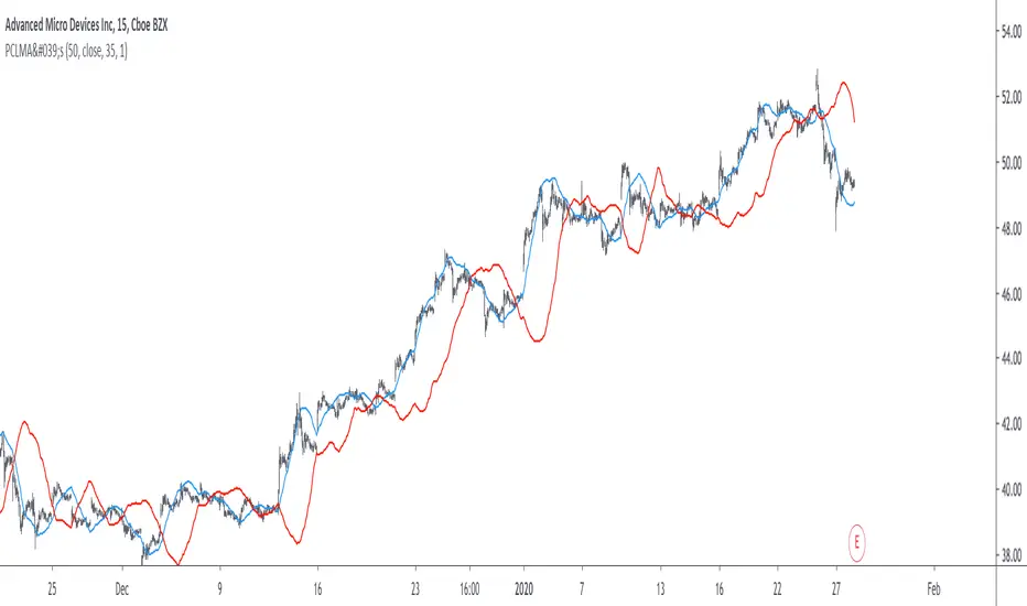
The indicator has two moving averages displayed on the chart, a trigger moving average (in blue) and a signal moving average (in red), their crosses can generate signals. The length parameter control the filter length, with higher values of length filtering longer term price fluctuations.
The percentage of negative weights parameter aim to determine the percentage of negative weights in the weighting function, note that the signal moving average won't use the same amount and will use instead : 100 - Percentage , this allow to reverse the weighting function thus creating a more lagging output for signal. Note that this parameter is caped at 50, this is because values higher than 50 would make the trigger moving average become the signal moving average, in short it inverse the role of the moving averages, that is a percentage of 25 would be the same than 75.
In red the moving average using 25% of negative weights, in blue the same moving average using 14% percent of negative weights. In theory, more negative weights = less lag = more overshoots.
Here the trigger MA in blue has 0% of negative weights, the trigger MA in green has however 35% of negative weights, the difference in lag can be clearly seen. In the case where there is 0% of negative weights the trigger become a simple WMA while the signal one become a moving average with linearly increasing weights.
The corrective factor is the same as alpha in PReLU, and determine the steepness of the negative weights line, this parameter is constrained in a range of (0,1), lower values will create a less steep negative weights line, this parameter is extremely useful when we want to reduce overshoots, an example :
here the corrective factor is equal to 1 (so the weighting function is an identity function) and we use 45% of negative weights, this create lot of overshoots, however a corrective factor of 0.5 reduce them drastically :
Center Of Linearity
The impulse response of the signal moving average is inverse to the impulse response of the trigger moving average, if we where to show them together we would see that they would crosses at a point, denoted center of linearity, therefore the crosses of each moving averages correspond to the cross of the center of linearity oscillator and 0 of same period.
This is also true with the center of gravity oscillator, linear covariance oscillator and linear correlation oscillator. Of course the center of linearity oscillator is way more efficient than the proposed indicator, and if a moving average crossover system is required, then the wma/sma pair is equivalent and way more efficient, who would know that i would propose something with more efficient alternatives ? xD
Estimating A Least Squares Moving Average
I guess...yeah...but its not my fault you know !!! Its a linear weighting function ! What can i do about it ?
The least squares moving average is corrective, its weighting function is linearly decreasing and posses negative weights with an amount of negative weights inferior to 50%, now we only need to find the exact percentage amount of negative weights. How to do it ? Well its not complicated if we recall the estimation with the WMA/SMA combination.
So, an LSMA of period p is equal to : 3WMA(p) - 2SMA(p) , each coefficient of the combination can give us this percentage, that is 2/3*100 = 33.333 , so there are 33.33% percent of negative weights in the weighting function of the least squares moving average.
In blue the trigger moving average with percentage of negative values et to 33.33, and in green the lsma of both period 50.
Conclusion
Altho inefficient, the proposed moving averages remain extremely interesting. They make use of the PReLU function as weighting function and allow the user to have a more accurate control over the characteristics of the moving averages output such as lag and overshoot amount, such parameters could even be made adaptive.
We have also seen how to estimate the least squares moving average, we have seen that the lsma posses 33.333...% of negative weights in its weighting function, another useful information.
The lsma is always behind me, not letting me focus on cryptobot super profit indicators using massive amount of labels, its like each time i make an indicator, the lsma come back, like a jealous creature, she want the center of attention, but you know well that the proposed indicator is inefficient ! Inefficient elegance (effect of the meds) .
Thanks for reading !
LSMA - A Fast And Simple Alternative CalculationIntroduction
At the start of 2019 i published my first post "Approximating A Least Square Moving Average In Pine", who aimed to provide alternatives calculation of the least squares moving average (LSMA), a moving average who aim to estimate the underlying trend in the price without excessive lag.
The LSMA has the form of a linear regression ax + b where x is a linear sequence 1.2.3..N and with time varying a and b , the exact formula of the LSMA is as follows :
a = stdev(close,length)/stdev(bar_index,length) * correlation(close,bar_index,length)
b = sma(close,length) - a*sma(bar_index,length)
lsma = a*bar_index + b
Such calculation allow to forecast future values however such forecast is rarely accurate and the LSMA is mostly used as a smoother. In this post an alternative calculation is proposed, such calculation is incredibly simple and allow for an extremely efficient computation of the LSMA.
Rationale
The LSMA is a FIR low-pass filter with the following impulse response :
The impulse response of a FIR filter gives us the weight of the filter, as we can see the weights of the LSMA are a linearly decreasing sequence of values, however unlike the linearly weighted moving average (WMA) the weights of the LSMA take on negative values, this is necessary in order to provide a better fit to the data. Based on such impulse response we know that the WMA can help calculate the LSMA, since both have weights representing a linearly decreasing sequence of values, however the WMA doesn't have negative weights, so the process here is to fit the WMA impulse response to the impulse response of the LSMA.
Based on such negative values we know that we must subtract the impulse response of the WMA by a constant value and multiply the result, such constant value can be given by the impulse response of a simple moving average, we must now make sure that the impulse response of the WMA and SMA cross at a precise point, the point where the impulse response of the LSMA is equal to 0.
We can see that 3WMA and 2SMA are equal at a certain point, and that the impulse response of the LSMA is equal to 0 at that point, if we proceed to subtraction we obtain :
Therefore :
LSMA = 3WMA - 2SMA = WMA + 2(WMA - SMA)
Comparison
On a graph the difference isn't visible, subtracting the proposed calculation with a regular LSMA of the same period gives :
the error is 0.0000000...and certainly go on even further, therefore we can assume that the error is due to rounding errors.
Conclusion
This post provided a different calculation of the LSMA, it is shown that the LSMA can be made from the linear combination of a WMA and a SMA : 3WMA + -2SMA. I encourage peoples to use impulse responses in order to estimate other moving averages, since some are extremely heavy to compute.
Thanks for reading !

Volume weighted LSMAQuick script made by reusing some functions written for other projects. This is a variation on the least squares moving average, but with custom weights on the linear regression. This gives higher weights to recent values and values with high volume.
Behaves very similarly to my volume weighted Hull moving average, especially with the hull smoothing option turned on.
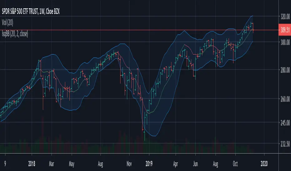
Least Squares Bollinger BandsSimilar to Bollinger Bands but adjusted for momentum. Instead of having the centerline be a simply moving average and the bands showing the rolling variance, this does a linear regression, and shows the LSMA at the center, while the band width is the average deviation from the regression line instead of from the SMA.
This means that unlike for normal Bollinger bands, momentum does not make the bands wider, and that the bands tend to be much better centered around the price action with band walks being more reliable indicators of undersold/oversold conditions. They also give a much narrower estimate of current volatility/price range.
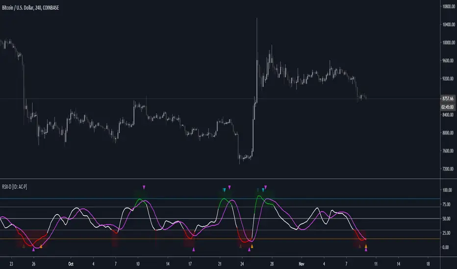
RSX-D [ID: AC-P]The "AC-P" version of Jaggedsoft's RSX Divergence and Everget's RSX script is my personal customized version of RSX with the following additions and modifications:
LSMA-D line that averages in three LSMA components to form a composite, the LSMA-D line. Offset for the LSMA-D line is set to -2 to offset latency from averaging togther the LSMA components to form a composite - recommended to adjust to your timeframe and asset/pair accordingly.
Divergence component from JustUncle, RicardoSantos, and Neobutane divergence scripts
Crossover indication and alerts for Midline, and custom M1 and M2 levels for both RSX and the LSMA-D line from Daveatt's CCI Stochastic Script
EMA21/55 zone cross highlighting option
SMA9/EMA45 MA option from my RSI sma/ema Cu script
Libertus Divergences and Pivot labels from Jaggedsoft's RSX Divergence script are hidden/off by default
Designed for darkmode by default. Minor visual changes from Jaggedsoft's and Everget's script(s) for darkmode and visual aesthetic.
Please Note:
Divergences that use fractal-based detection logic, offset, or a combination of both generally have a 1-2 bar/candle lag. This is an INHERENT limitation of divergence detection with fractals and offsets. Divergences generally will have a higher strikerate on HTF than LTF due to the 1-2 bar lag. While I'm not going to rule out a programming solution or math construct/formula that attempts to alleivates the 1-2 bar lag for divergences, this script is not it - please keep that in mind when using divergence components with a fractal base and offset.
LSMA-D is a composite of three LSMA lines, all with offset options. Different lengths and Offset values can compensate/adjust for the smoothing/latency from RSX, but only up to a certain point. For each LSMA, the least square regression line is calculated for the previous time periods, so the idea is that with finely tuned adjustments, you can get crossover/crossunder signals from the RSX with the LSMA-D line that you simply can't get with the SMA9/EMA45 due to the already smoothed RSX.
The defaults for the RSX and various components for the LSMA-D here will MOSTLY LIKELY NOT WORK OR BE APPLICABLE to every timeframe and asset that you trade - adjust, backtest, and test accordingly. The defaults are here are MEANT to be adjusted to the asset class and timeframe that you are trading.
If you're not familiar with the LSMA, tradingview author Alexgrover has a few great scripts that go into detail how the LSMA works, in addition to different interpretations and implementations of the LSMA.
References/Acknowledgements:
//@version=4
// Copyright (c) 2019-present, Alex Orekhov (everget)
// Jurik RSX script may be freely distributed under the MIT license.
//
//-------------------------------------------------------------------
// Acknowledgements:
//---- Base script:
// RSX Divergence — SharkCIA by Jaggedsoft
//
// Jurik Moving Average by Everget
//
//---- Divergences/Signals:
// Libertus RSI Divergences
//
// Price Divergence Dectector V3 by JustUncle
//
// Price Divergence Detector V2 by RicardoSantos
//
// Stochastic RSI with Divergences by Neobutane
//
// CCI Stochastic by Daveatt
//
//---- Misc. Reference:
// RSI SMA/EMA Cu by Auroagwei
//
// CBCI Cu by Auroagwei
//
// Chop and explode by fhenry0331
//
// T-Step LSMA by RafaelZioni
//
// Scripts by Jaggedsoft for structure and formatting
// Scripts by Everget for structure and formatting
//-------------------------------------------------------------------
// RSX-D v08
// Author: Auroagwei
// www.tradingview.com
//-------------------------------------------------------------------
Quadratic Least Squares Moving Average - Smoothing + Forecast Introduction
Technical analysis make often uses of classical statistical procedures, one of them being regression analysis, and since fitting polynomial functions that minimize the sum of squares can be achieved with the use of the mean, variance, covariance...etc, technical analyst only needed to replace the mean in all those calculations with a moving average, we then end up with a low lag filter called least squares moving average (lsma) .
The least squares moving average could be classified as a rolling linear regression, altho this sound really bad it is useful to understand the relationship of both methods, both have the same form, that is ax + b , where a and b are coefficients of the model. However in a simple linear regression a and b are constant, while the lsma use variables instead.
In a simple lsma we model the relationship of the closing price (dependent variable) with a linear sequence (independent variable), therefore x = 1,2,3,4..etc. However we can use polynomial of higher degrees to model such relationship, this is required if we want more reactivity. Therefore we can use a quadratic form, that is ax^2 + bx + c , where a,b and c are variables.
This is the quadratic least squares moving average (qlsma), a not so official term, but we'll stick with it because it still represent the aim of the filter quite well. In this indicator i make the calculations of the qlsma less troublesome, therefore one might understand how it would work, note that in general the coefficients of a polynomial regression model are found using matrix calculus.
The Indicator
A qlsma, unlike the classic lsma, will fit better to the price and will be more reactive, this is the advantage of using an higher degrees for its calculation, we can model more complex relationship.
lsma in green, qlsma in red, with both length = 200
However the over/under shoots are greater, i'll explain why in the next sections, but this is one of the drawbacks of using higher degrees.
The indicator allow to forecast future values, the ahead period of the forecast is determined by the forecast setting. The value for this setting should be lower than length, else the forecasts can easily over/under shoot which heavily damage the forecast. In order to get a view on how well the forecast is performing you can check the option "Show past predicted values".
Of course understanding the logic behind the forecast is important, in short regressions models best fit a certain curve to the data, this curve can be a line (linear regression), a parabola (quadratic regression) and so on, the type of curve is determined by the degree of the polynomial used, here 2, which is a parabola. Lets use a linear regression model as example :
ax + b where x is a linear sequence 1,2,3...and a/b are constants. Our goal is to find the values for a and b that minimize the sum of squares of the line with the dependent variable y, here the closing price, so our hypothesis is that :
closing price = ax + b + ε
where ε is white noise, a component that the model couldn't forecast. The forecast of the closing price 14 step ahead would be equal to :
closing price 14 step aheads = a(x+14) + b
Since x is a linear sequence we only need to sum it with the forecasting horizon period, the same is done here with :
a*(n+forecast)^2 + b*(n + forecast) + c
Note that the forecast proposed in the indicator is more for teaching purpose that anything else, this indicator can't possibly forecast future values, even on a meh rate.
Low lag filters have been used to provide noise free crosses with slow moving average, a bad practice in my opinion due to the ability low lag filters have to overshoot/undershoot, more interesting use cases might be to use the qlsma as input for other indicators.
On The Code
Some of you might know that i posted a "quadratic regression" indicator long ago, the original calculations was coming from a forum, but because the calculation was ugly as hell as well as extra inefficient (dogfood level) i had to do something about it, the name was also terribly misleading.
We can see in the code that we make heavy use of the variance and covariance, both estimated with :
VAR(x) = SMA(x^2) - SMA(x)^2
COV(x,y) = SMA(xy) - SMA(x)SMA(y)
Those elements are then combined, we can easily recognize the intercept element c , who don't change much from the classical lsma.
As Digital Filter
The frequency response of the qlsma is similar to the one of the lsma, those filters amplify certain frequencies in the passband, and have ripples in the stop band. There is something interesting about those filters, first using higher degrees allow to greater boost of the frequencies in the passband, which result in greater over/under shoots. Another funny thing is that the peak/valley of the ripples is equal the peak or valley in the ripples of another lsma of different degree.
The transient response of those filters, that is impulse response, step response...etc is related to the degree of the polynomial used, therefore lets denote a lsma of degree p : lsma(p) , the impulse response of lsma(p) is a polynomial of degree p, and the step response is simple a polynomial of order p+1.
This is why it was more interesting to estimate the qlsma using convolution, however we can no longer forecast future values.
Conclusion
I proposed a more usable quadratic least squares moving average, with more options, as well as a cleaner and more efficient code. The process of shrinking the original code is made easier when you know about the estimations of both variance and covariance.
I hope the proposed indicator/calculation is useful.
Thx for reading !

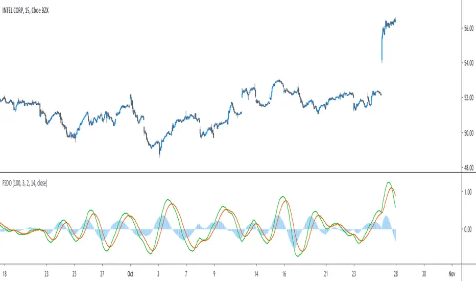
Fast/Slow Degree OscillatorIntroduction
The estimation of a least squares moving average of any degree isn't an interesting goal, this is due to the fact that lsma of high degrees would highly overshoot as well as overfit the closing price, which wouldn't really appear smooth. However i proposed an estimate of an lsma of any degree using convolution and a new sine wave series, all the calculation are described in the paper : "Pierrefeu, Alex (2019): A New Low-Pass FIR Filter For Signal Processing."
Today i want to make use of this filter as an oscillator providing fast entry points. The oscillator would be similar to the MACD in the sense that is consist on the difference between two filters, with one faster than the other, however unlike the MACD which use two moving averages of different length, here i'll use two filters of same length but different degrees.
The Indicator
The indicator consist in 3 elements, one main line (in green) the trigger line (in orange) and the histogram which is the difference between the green line and the red one. The main line is made from the difference between two filters of both period length and different degrees (fast, slow), fast should always be higher than slow. The signal line is just the exponential moving average of the main line, the period of the exponential moving average can be adjusted from the settings.
Both fast/slow determine the degree of the filters, higher values will create a faster filter.
For those who are curious, the filter use a kernel who estimate a polynomial function, this is how an lsma work, the kernel of an lsma of degree p is a polynomial of degree p . I achieved this estimation using a sine wave series.
When fast = 1 and slow = 0, the oscillator appear less periodic, this equivalent to : lsma - sma
Using 2/1 allow the indicator to highlight cycles more easily without being uncorrelated with the price. This is equivalent to qlsma - lsma, where qlsma is a quadratic least squares moving average. This is similar to my old indicator "Linear Quadratic Convergence Divergence Oscillator".
By default the indicator use 3 for fast and 2 for slow, but you can increase both values, here 4/3 :
In general higher values of fast/slow will create way more cyclical results, but they can be uncorrelated with the market price.
Conclusion
This indicator was rather made to show the filter calculation rather than proposing something interesting. However it can be funny to see how the difference between low lag filters create more cyclical outputs, it often allow indicators to have more predictive capabilities.
I invite you to read the paper made about the filter, codes for both pinescript and python are provided.
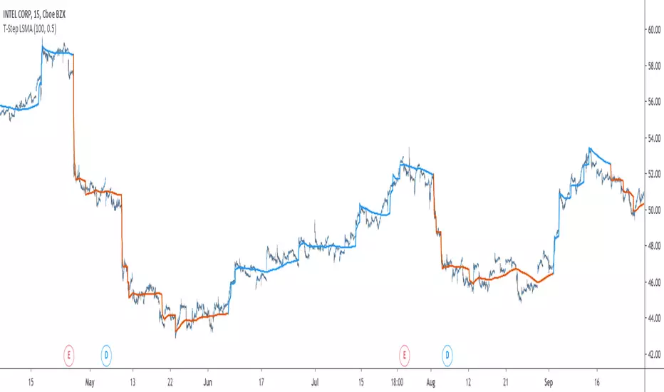
T-Step LSMAIntroduction
The trend step indicator family has produced much interest in the community, those indicators showed in certain cases robustness and reactivity. Their ease of use/interpretation is also a major advantage. Although those indicators have a relatively good fit with the input price, they can still be improved by introducing least-squares fitting on their calculations. This is why i propose a new indicator (T-Step LSMA) which aim to gather all the components of the trend-step indicator family (including the auto-line family).
The indicator will use as a threshold the mean absolute error between the input and the output (T-Channel) scaled with the efficiency ratio (Efficient Trend Step) while using least squares in order to provide a better fit with the price (Auto-Filter).
The Indicator
The interpretation of the indicator is easy, the indicator estimate an up-trending market when in blue, down-trending when in orange, the signal only depend on the trend-step part ( b in the code).
length control the period of the efficiency ratio as well as any components in the lsma calculation. The efficiency ratio allow to provide adaptivity, therefore the threshold will be lower when market is trending and higher when market is ranging.
Sc control the amount of feedback of the indicator, a value of 1 will use only the closing price as input, a value of 0.5 will use 50% of the closing price/indicator output as input, this allow to get smoother results.
It is possible to get the non-smooth version of the indicator by checking "No Smoothing".
This allow the indicator to filter more information.
Least Squares Smoothing - Benefits
One could ask why introducing least squares smoothing, there are several reasons to this choice, we have seen that trend-step indicators are boxy, they filter most of the variational information in the price, introducing least squares smoothing allow to gain back some of this variational information while providing a better fit with the price, the indicator is more noisy but also more practical in certain situations.
For example the indicator in its boxy form can't really be useful as input for other indicators, which is not the case with this version.
Relative strength index of period 14 using the proposed indicator as input.
Down-Sides
The indicator is dependent on the time frame used, larger time frames resulting in an indicator overfitting, sticking with lower time frames might be ideal. The indicator behavior might also change depending on the market in which it is applied.
Setting Up Alerts For The Indicator
Alerts conditions are already set, in order to create an alert based on the indicator follow these steps :
Go to the alert section (the alarm clock) -> create new alert -> select T-Step LSMA in condition -> Below select Up or Dn (Up for a up-trending alert and Dn for a down-trending alert)
In option select "once per bar close", change the message if you want a personalized message.
Conclusion
I don't think i'll post other indicators related to the trend-step framework for the time to comes, nonetheless the ones posted proven to have interesting results as well as many upsides. Although i don't think they would generate positive long-terms returns they could still be of use when using smarter volatility metrics as threshold. The proposed indicator conserve more information than its relatives and might find some use as input for other indicators.
Recommended Use Of The Code
Although i don't put restrictions on the code usage, i still recommend creative and pertinent changes to be made, graphical changes or any minor changes are not necessary, remember that such practice is disrespectful toward the author, you don't want to load up the tradingview servers for nothing right ?
Support Me
Making indicators sure is hard, it takes time and it can be quite lonely to, so i would love talking with you guys while making them :) There isn't better support than the one provided by your friends so drop me a message.
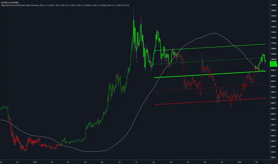
Regression Channel [DW]This is an experimental study which calculates a linear regression channel over a specified period or interval using custom moving average types for its calculations.
Linear regression is a linear approach to modeling the relationship between a dependent variable and one or more independent variables.
In linear regression, the relationships are modeled using linear predictor functions whose unknown model parameters are estimated from the data.
The regression channel in this study is modeled using the least squares approach with four base average types to choose from:
-> Arnaud Legoux Moving Average (ALMA)
-> Exponential Moving Average (EMA)
-> Simple Moving Average (SMA)
-> Volume Weighted Moving Average (VWMA)
When using VWMA, if no volume is present, the calculation will automatically switch to tick volume, making it compatible with any cryptocurrency, stock, currency pair, or index you want to analyze.
There are two window types for calculation in this script as well:
-> Continuous, which generates a regression model over a fixed number of bars continuously.
-> Interval, which generates a regression model that only moves its starting point when a new interval starts. The number of bars for calculation cumulatively increases until the end of the interval.
The channel is generated by calculating standard deviation multiplied by the channel width coefficient, adding it to and subtracting it from the regression line, then dividing it into quartiles.
To observe the path of the regression, I've included a tracer line, which follows the current point of the regression line. This is also referred to as a Least Squares Moving Average (LSMA).
For added predictive capability, there is an option to extend the channel lines into the future.
A custom bar color scheme based on channel direction and price proximity to the current regression value is included.
I don't necessarily recommend using this tool as a standalone, but rather as a supplement to your analysis systems.
Regression analysis is far from an exact science. However, with the right combination of tools and strategies in place, it can greatly enhance your analysis and trading.
Kaufman Adaptive Least Squares Moving AverageIntroduction
It is possible to use a wide variety of filters for the estimation of a least squares moving average, one of the them being the Kaufman adaptive moving average (KAMA) which adapt to the market trend strength, by using KAMA in an lsma we therefore allow for an adaptive low lag filter which might provide a smarter way to remove noise while preserving reactivity.
The Indicator
The lsma aim to minimize the sum of the squared residuals, paired with KAMA we obtain a great adaptive solution for smoothing while conserving reactivity. Length control the period of the efficiency ratio used in KAMA, higher values of length allow for overall smoother results. The pre-filtering option allow for even smoother results by using KAMA as input instead of the raw price.
The proposed indicator without pre-filtering in green, a simple moving average in orange, and a lsma with all of them length = 200. The proposed filter allow for fast and precise crosses with the moving average while eliminating major whipsaws.
Same setup with the pre-filtering option, the result are overall smoother.
Conclusion
The provided code allow for the implementation of any filter instead of KAMA, try using your own filters. Thanks for reading :)
Polynomial LSMA Estimation - Estimating An LSMA Of Any DegreeIntroduction
It was one of my most requested post, so here you have it, today i present a way to estimate an LSMA of any degree by using a kernel based on a sine wave series, note that this is originally a paper that i posted that you can find here figshare.com , in the paper you will be able to find the frequency response of the filter as well as both python and pinescript code.
The least squares moving average or LSMA is a filter that best fit a polynomial function through the price by using the method of least squares, by default the LSMA best fit a line through the input by using the following formula : ax + b where x is often a linear series 1,2,3...etc and a/b are parameters, the LSMA is made by finding a and b such that their values minimize the sum of squares between the lsma and the input.
Now a LSMA of 2nd degree (quadratic) is in the form of ax^2 + bx + c , although the first order LSMA is not hard to make the 2nd order one is way more heavy in term of codes since we must find optimal values for a , b and c , therefore we may want to find alternatives if the goal is simply data smoothing.
Estimation By Convolution
The LSMA is a FIR filter which posses various characteristics, the impulse response of an LSMA of degree n is a polynomial of the same degree, and its step response is a polynomial of degree n+1, estimating those step response is done by the described sine wave series :
f(x) =>
sum = 0.
b = 0.
pi = atan(1)*4
a = x*x
for i = 1 to d
b := 1/i * sin(x*i*pi)
sum := sum + b
pol = a + iff(d == 0,0,sum)
which is simple the sum of multiple sine waves of different frequency and amplitude + the square of a linear function. We then differentiate this result and apply convolution.
The Indicator
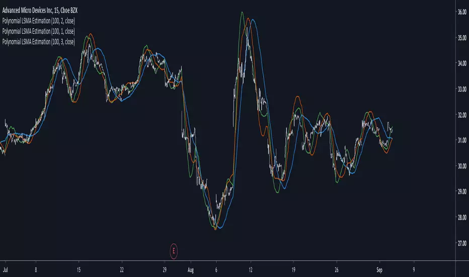
length control the filter period while degree control the degree of the filter, higher degree's create better fit with the input as seen below :
Now lets compare our estimate with actual LSMA's, below a lsma in blue and our estimate in orange of both degree 1 and period 100 :
Below a LSMA of degree 2 (quadratic) and our estimate with degree 2 with both period 100 :
It can be seen that the estimate is doing a pretty decent job.
Now we can't make comparisons with higher degrees of lsma's but thats not a real necessity.
Conclusion
This indicator wasn't intended as a direct estimate of the lsma but it was originally based on the estimation of polynomials using sine wave series, which led to the proposed filter showcased in the article. So i think we can agree that this is not a bad estimate although i could have showcased more statistics but thats to many work, but its not that interesting to use higher degree's anyways so sticking with degree 1, 2 and 3 might be for the best.
Hope you like and thanks for reading !
Options - Kaufman / LEAST SQUARES Moving AverageThis is a combo of multiple indicators :
1- three kama moving averages
2- one lsma moving average
3- a kama upper and lower band that you can set to use any of the three kama moving averages in the indicator as source
4- upper, lower and center bollinger bands price for last candle
The horizontal dot line is the bollinger and the horizontal arrowed lines are the bands for kama indicator.
The parameters are available for KAMA, LSMA and BB settings, the default settings are prefabricated for options trading.

Time Series ForecastIntroduction
Forecasting is a blurry science that deal with lot of uncertainty. Most of the time forecasting is made with the assumption that past values can be used to forecast a time series, the accuracy of the forecast depend on the type of time series, the pre-processing applied to it, the forecast model and the parameters of the model.
In tradingview we don't have much forecasting models appart from the linear regression which is definitely not adapted to forecast financial markets, instead we mainly use it as support/resistance indicator. So i wanted to try making a forecasting tool based on the lsma that might provide something at least interesting, i hope you find an use to it.
The Method
Remember that the regression model and the lsma are closely related, both share the same equation ax + b but the lsma will use running parameters while a and b are constants in a linear regression, the last point of the lsma of period p is the last point of the linear regression that fit a line to the price at time p to 1, try to add a linear regression with count = 100 and an lsma of length = 100 and you will see, this is why the lsma is also called "end point moving average".
The forecast of the linear regression is the linear extrapolation of the fitted line, however the proposed indicator forecast is the linear extrapolation between the value of the lsma at time length and the last value of the lsma when short term extrapolation is false, when short term extrapolation is checked the forecast is the linear extrapolation between the lsma value prior to the last point and the last lsma value.
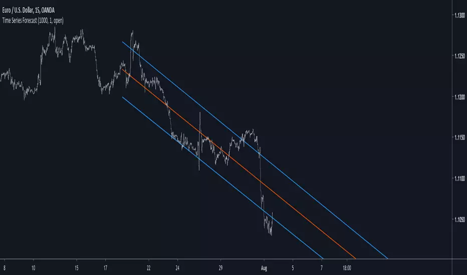
long term extrapolation, length = 1000
short term extrapolation, length = 1000
How To Use
Intervals are create from the running mean absolute error between the price and the lsma. Those intervals can be interpreted as possible support and resistance levels when using long term extrapolation, make sure that the intervals have been priorly tested, this mean the intervals are more significants.
The short term extrapolation is made with the assumption that the price will follow the last two lsma points direction, the forecast tend to become inaccurate during a trend change or when noise affect heavily the lsma.
You can test both method accuracy with the replay mode.
Comparison With The Linear Regression
Both methods share similitudes, but they have different results, lets compare them.
In blue the indicator and in red a linear regression of both period 200, the linear regression is always extremely conservative since she fit a line using the least squares method, at the contrary the indicator is less conservative which can be an advantage as well as a problem.
Conclusion
Linear models are good when what we want to forecast is approximately linear, thats not the case with market price and this is why other methods are used. But the use of the lsma to provide a forecast is still an interesting method that might require further studies.
Thanks for reading !
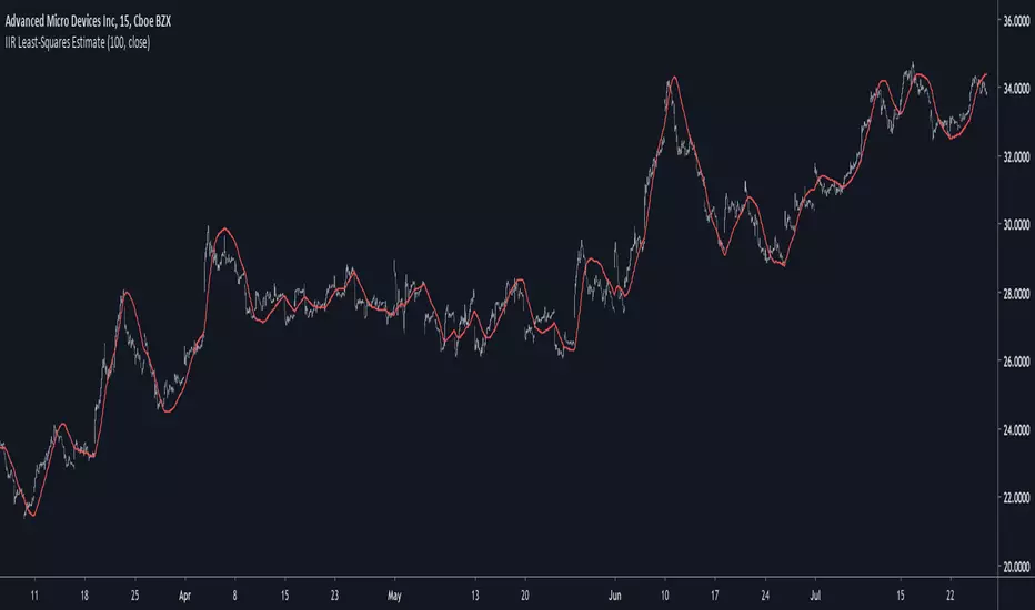
IIR Least-Squares EstimateIntroduction
Another lsma estimate, i don't think you are surprised, the lsma is my favorite low-lag filter and i derived it so many times that our relationship became quite intimate. So i already talked about the classical method, the line-rescaling method and many others, but we did not made to many IIR estimate, the only one was made using a general filter estimator and was pretty inaccurate, this is why i wanted to retry the challenge.
Before talking about the formula lets breakdown again what IIR mean, IIR = infinite impulse response, the impulse response of an IIR filter goes on forever, this is why its infinite, such filters use recursion, this mean they use output's as input's, they are extremely efficient.
The Calculation
The calculation is made with only 1 pole, this mean we only use 1 output value with the same index as input, more poles often means a transition band closer to the cutoff frequency.
Our filter is in the form of :
y = a*x+y - a*ema(y,length/2)
where y = x when t = 1 and y(1) when t > 2 and a = 4/(length+2)
This is also an alternate form of exponential moving average but smoothing the last output terms with another exponential moving average reduce the lag.
Comparison
Lets see the accuracy of our estimate.
Sometimes our estimate follow better the trend, there isn't a clear result about the overshoot/undershoot response, sometimes the estimate have less overshoot/undershoot and sometime its the one with the highest.
The estimate behave nicely with short length periods.
Conclusion
Some surprises, the estimate can at least act as a good low-lag filter, sometimes it also behave better than the lsma by smoothing more. IIR estimate are harder to make but this one look really correct.
If you are looking for something or just want to say thanks try to pm me :)
Thank for reading !
Fisher Least Squares Moving AverageIntroduction
I already estimated the least-squares moving average numerous times, one of the most elegant ways was by rescaling a linear function to the price by using the z-score, today i will propose a new smoother (FLSMA) based on the line rescaling approach and the inverse fisher transform of a scaled moving average error with the goal to provide an alternative least-squares smoother, the indicator won't use the correlation coefficient and will try to adresses problems such as overshoots and lag reduction.
Line Rescaling Method
For those who did not see my least squares moving average estimation using the line rescaling method here is a resume, we want to fit a polynomial function of degree 1 to the price by reducing the sum of squares between the price and the filter, squares is a term meaning the squared difference between the price and its estimation. The line rescaling technique work as follow :
1 - get the z-score of a line.
2 - multiply this z-score with the correlation between the price and a line.
3 - multiply the precedent result with the standard deviation of the price, then sum that to a simple moving average.
This process is shorter than the classical least-squares moving average method.
Z-Score Derivation And The Inverse Fisher Transform
The FLSMA will use a similar approach to the line rescaling technique but instead of using the correlation during step 2 we will use an alternative calculated from the error between the estimate and the price.
In order to do so we must use the inverse fisher transform, the inverse fisher transform can take a z-score and scale it in a range of (1,-1), it is possible to estimate the correlation with it. First lets create our modified z-score in the form of : Z = ma((y - Y)/e) where y is the price, Y our output estimate and e the moving average absolute error between the price and Y and lets call it scaled smoothed error , then apply the inverse fisher transform : r = IFT(Z) = tanh(Z) , we then multiply the z-score of the line with it.
Performance
The FLSMA greatly reduce the overshoots, this mean that the maximas of abs(r) are lower than the maxima's of the absolute correlation, such case is not "bad" but we can see that the filter is not closer to the price than the LSMA during trending periods, we can assume the filter don't reduce least-squares as well as the LSMA.
The image above is the running mean of the absolute error of each the FLSMA (in red) and the LSMA (in blue), we could fix this problem by multiplying the smooth scaled error by p where p can be any number, for example :
z = sma(src - nz(b ,src),length)/e * p where p = 2
In red the FLSMA and in blue the FLSMA with p = 2 , the greater p is the less lag the FLSMA will have.
Conclusion
It could be possible to get better results than the LSMA with such design, the presented indicator use its own correlation replacement but it is possible to use anything in a range of (1,-1) to multiply the line z-score. Although the proposed filter only reduce overshoots without keeping the accuracy of the LSMA i believe the code can be useful for others.
Thanks for reading.

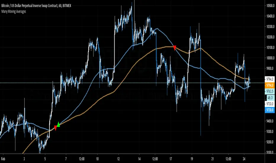
Many Moving AveragesThis script allows you to add two moving averages to a chart, where the type of moving average can be chosen from a collection of 15 different moving average algorithms. Each moving average can also have different lengths and crossovers/unders can be displayed and alerted on.
The supported moving average types are:
Simple Moving Average ( SMA )
Exponential Moving Average ( EMA )
Double Exponential Moving Average ( DEMA )
Triple Exponential Moving Average ( TEMA )
Weighted Moving Average ( WMA )
Volume Weighted Moving Average ( VWMA )
Smoothed Moving Average ( SMMA )
Hull Moving Average ( HMA )
Least Square Moving Average/Linear Regression ( LSMA )
Arnaud Legoux Moving Average ( ALMA )
Jurik Moving Average ( JMA )
Volatility Adjusted Moving Average ( VAMA )
Fractal Adaptive Moving Average ( FRAMA )
Zero-Lag Exponential Moving Average ( ZLEMA )
Kauman Adaptive Moving Average ( KAMA )
Many of the moving average algorithms were taken from other peoples' scripts. I'd like to thank the authors for making their code available.
JayRogers
Alex Orekhov (everget)
Alex Orekhov (everget)
Joris Duyck (JD)
nemozny
Shizaru
KobySK
Jurik Research and Consulting for inventing the JMA.
R2-Adaptive RegressionIntroduction
I already mentioned various problems associated with the lsma, one of them being overshoots, so here i propose to use an lsma using a developed and adaptive form of 1st order polynomial to provide several improvements to the lsma. This indicator will adapt to various coefficient of determinations while also using various recursions.
More In Depth
A 1st order polynomial is in the form : y = ax + b , our indicator however will use : y = a*x + a1*x1 + (1 - (a + a1))*y , where a is the coefficient of determination of a simple lsma and a1 the coefficient of determination of an lsma who try to best fit y to the price.
In some cases the coefficient of determination or r-squared is simply the squared correlation between the input and the lsma. The r-squared can tell you if something is trending or not because its the correlation between the rough price containing noise and an estimate of the trend (lsma) . Therefore the filter give more weight to x or x1 based on their respective r-squared, when both r-squared is low the filter give more weight to its precedent output value.
Comparison
lsma and R2 with both length = 100
The result of the R2 is rougher, faster, have less overshoot than the lsma and also adapt to market conditions.
Longer/Shorter terms period can increase the error compared to the lsma because of the R2 trying to adapt to the r-squared. The R2 can also provide good fits when there is an edge, this is due to the part where the lsma fit the filter output to the input (y2)
Conclusion
I presented a new kind of lsma that adapt itself to various coefficient of determination. The indicator can reduce the sum of squares because of its ability to reduce overshoot as well as remaining stationary when price is not trending. It can be interesting to apply exponential averaging with various smoothing constant as long as you use : (1- (alpha+alpha1)) at the end.
Thanks for reading

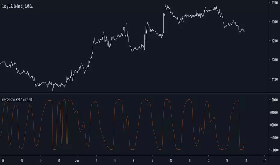
Inverse Fisher Fast Z-scoreIntroduction
The fast z-score is a modification of the classic z-score that allow for smoother and faster results by using two least squares moving averages, however oscillators of this kind can be hard to read and modifying its shape to allow a better interpretation can be an interesting thing to do.
The Indicator
I already talked about the fisher transform, this statistical transform is originally applied to the correlation coefficient, the normal transform allow to get a result similar to a smooth z-score if applied to the correlation coefficient, the inverse transform allow to take the z-score and rescale it in a range of (1,-1), therefore the inverse fisher transform of the fast z-score can rescale it in a range of (1,-1).
inverse = (exp(k*fz) - 1)/(exp(k*fz) + 1)
Here k will control the squareness of the output, an higher k will return heavy side step shapes while a lower k will preserve the smoothness of the output.
Conclusion
The fisher transform sure is useful to kinda filter visual information, it also allow to draw levels since the rescaling is in a specific range, i encourage you to use it.
Notes
During those almost 2 weeks i was even lazier and sadder than ever before, so i think its no use to leave, i also have papers to publish and i need tv for that.
Thanks for reading !
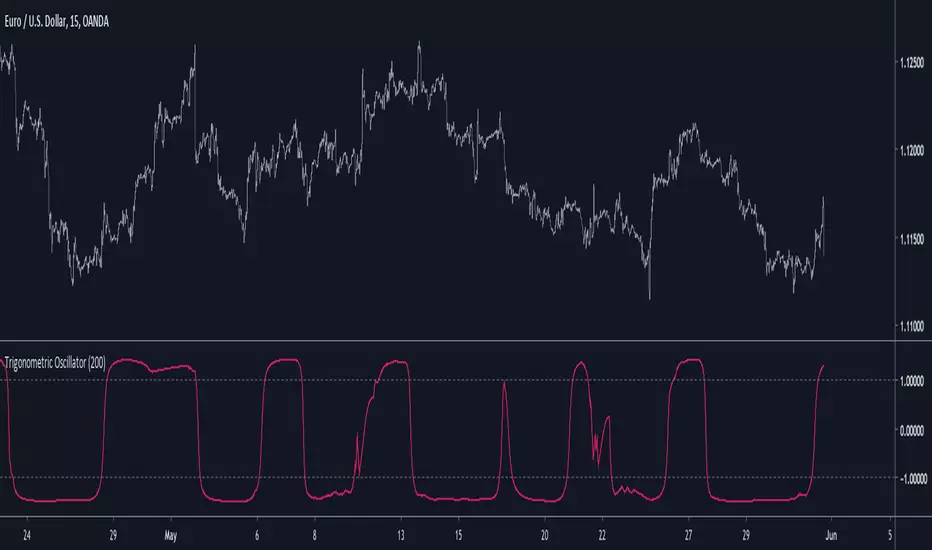
Trigonometric OscillatorIts a pretty old script and i have absolutely no idea how i did it, the code kinda look like the phase wrapping/unwrapping formula. This indicator is an oscillator, sometimes its reactivity is impressive so i think its a good idea to post it, feel free to experiment with it.
Well Rounded Moving AverageIntroduction
There are tons of filters, way to many, and some of them are redundant in the sense they produce the same results as others. The task to find an optimal filter is still a big challenge among technical analysis and engineering, a good filter is the Kalman filter who is one of the more precise filters out there. The optimal filter theorem state that : The optimal estimator has the form of a linear observer , this in short mean that an optimal filter must use measurements of the inputs and outputs, and this is what does the Kalman filter. I have tried myself to Kalman filters with more or less success as well as understanding optimality by studying Linear–quadratic–Gaussian control, i failed to get a complete understanding of those subjects but today i present a moving average filter (WRMA) constructed with all the knowledge i have in control theory and who aim to provide a very well response to market price, this mean low lag for fast decision timing and low overshoots for better precision.
Construction
An good filter must use information about its output, this is what exponential smoothing is about, simple exponential smoothing (EMA) is close to a simple moving average and can be defined as :
output = output(1) + α(input - output(1))
where α (alpha) is a smoothing constant, typically equal to 2/(Period+1) for the EMA.
This approach can be further developed by introducing more smoothing constants and output control (See double/triple exponential smoothing - alpha-beta filter) .
The moving average i propose will use only one smoothing constant, and is described as follow :
a = nz(a ) + alpha*nz(A )
b = nz(b ) + alpha*nz(B )
y = ema(a + b,p1)
A = src - y
B = src - ema(y,p2)
The filter is divided into two components a and b (more terms can add more control/effects if chosen well) , a adjust itself to the output error and is responsive while b is independent of the output and is mainly smoother, adding those components together create an output y , A is the output error and B is the error of an exponential moving average.
Comparison
There are a lot of low-lag filters out there, but the overshoots they induce in order to reduce lag is not a great effect. The first comparison is with a least square moving average, a moving average who fit a line in a price window of period length .
Lsma in blue and WRMA in red with both length = 100 . The lsma is a bit smoother but induce terrible overshoots
ZLMA in blue and WRMA in red with both length = 100 . The lag difference between each moving average is really low while VWRMA is way more precise.
Hull MA in blue and WRMA in red with both length = 100 . The Hull MA have similar overshoots than the LSMA.
Reduced overshoots moving average (ROMA) in blue and WRMA in red with both length = 100 . ROMA is an indicator i have made to reduce the overshoots of a LSMA, but at the end WRMA still reduce way more the overshoots while being smoother and having similar lag.
I have added a smoother version, just activate the extra smooth option in the indicator settings window. Here the result with length = 200 :
This result is a little bit similar to a 2 order Butterworth filter. Our filter have more overshoots which in this case could be useful to reduce the error with edges since other low pass filters tend to smooth their amplitude thus reducing edge estimation precision.
Conclusions
I have presented a well rounded filter in term of smoothness/stability and reactivity. Try to add more terms to have different results, you could maybe end up with interesting results, if its the case share them with the community :)
As for control theory i have seen neural networks integrated to Kalman flters which leaded to great accuracy, AI is everywhere and promise to be a game a changer in real time data smoothing. So i asked myself if it was possible for a neural networks to develop pinescript indicators, if yes then i could be replaced by AI ? Brrr how frightening.
Thanks for reading :)