Fractal Fade Pro IndicatorA revolutionary contrarian trading indicator that applies chaos theory, fractal mathematics, and market entropy to generate high-probability reverse signals. This indicator fades traditional technical signals, providing BUY signals when conventional indicators say SELL, and SELL signals when they say BUY.
Full Description:
Most traders follow the herd. QFCI does the opposite. It identifies when conventional technical analysis is about to fail by detecting mathematical patterns of exhaustion in market structure.
How It Works (Technical Overview):
The indicator combines three sophisticated mathematical approaches:
Fractal Dimension Analysis: Measures the "roughness" of price movements using fractal mathematics
Market Entropy Calculation: Quantifies the randomness and disorder in price returns using information theory
Phase Space Reconstruction: Analyzes price evolution in multi-dimensional state space from chaos theory
Signal Generation Process:
Step 1: Market Regime Detection
Chaotic Regime: High fractal complexity + rising entropy (avoid trading)
Trending Regime: Low fractal complexity + high phase space distance (fade breakouts)
Mean-Reverting Regime: Very low fractal complexity (fade extremes)
Step 2: Reverse Signal Logic
When traditional indicators would give:
BUY signal (breakout, oversold bounce, volatility spike) → QFCI shows SELL
SELL signal (breakdown, overbought rejection, volatility crash) → QFCI shows BUY
Step 3: Smart Signal Filtering
No consecutive same-direction signals
Adjustable minimum bars between signals
Multiple confirmation layers required
Unique Features:
1. Mathematical Innovation:
Original fractal dimension algorithm (not standard indicators)
Market entropy calculation from information theory
Phase space reconstruction from chaos theory
Multi-regime adaptive logic
2. Trading Psychology Advantage:
Contrarian by design - profits from market overreactions
Fades retail trader mistakes - enters when others are exiting
Reduces overtrading - strict signal frequency controls
3. Clean Visual Interface:
Only BUY/SELL labels - no chart clutter
Clear directional arrows - immediate signal recognition
Built-in alerts - never miss a trade
Recommended Settings:
Default (Balanced Approach):
Fractal Depth: 20
Entropy Period: 200
Min Bars Between Signals: 100
Aggressive Trading:
Fractal Depth: 10-15
Entropy Period: 100-150
Min Bars Between Signals: 50-75
Conservative Trading:
Fractal Depth: 30-40
Entropy Period: 300-400
Min Bars Between Signals: 150-200
Optimal Timeframes:
Primary: Daily, Weekly (best performance)
Secondary: 4-Hour, 12-Hour
Can work on: 1-Hour (with adjusted parameters)
How to Use:
For Beginners:
Apply indicator to chart
Use default settings
Wait for BUY/SELL labels
Enter on next candle open
Use 2:1 risk/reward ratio
Always use stop losses
For Advanced Traders:
Adjust parameters for your trading style
Combine with support/resistance levels
Use volume confirmation
Scale in/out of positions
Track performance by regime
Risk Management Guidelines:
Position Sizing:
Conservative: 1-2% risk per trade
Moderate: 2-3% risk per trade
Aggressive: 3-5% risk per trade (not recommended)
Stop Loss Placement:
BUY signals: Below recent swing low or -2x ATR
SELL signals: Above recent swing high or +2x ATR
Take Profit Targets:
Primary: 2x risk (minimum)
Secondary: Previous support/resistance
Tertiary: Trailing stops after 1.5x risk
IMPORTANT RISK DISCLOSURE
This indicator is for educational and informational purposes only. It is not financial advice. Past performance does not guarantee future results. Trading involves substantial risk of loss and is not suitable for every investor. The risk of loss in trading can be substantial. You should therefore carefully consider whether such trading is suitable for you in light of your financial condition.
Mathematical

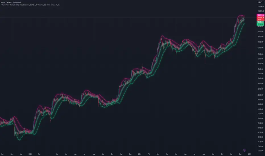
FIR Low Pass Filter Suite (FIR)The FIR Low Pass Filter Suite is an advanced signal processing indicator that applies finite impulse response (FIR) filtering techniques to price data. At its core, the indicator uses windowed-sinc filtering, which provides optimal frequency response characteristics for separating trend from noise in financial data.
The indicator offers multiple window functions including Kaiser, Kaiser-Bessel Derived (KBD), Hann, Hamming, Blackman, Triangular, and Lanczos. Each window type provides different trade-offs between main-lobe width and side-lobe attenuation, allowing users to fine-tune the frequency response characteristics of the filter. The Kaiser and KBD windows provide additional control through an alpha parameter that adjusts the shape of the window function.
A key feature is the ability to operate in either linear or logarithmic space. Logarithmic filtering can be particularly appropriate for financial data due to the multiplicative nature of price movements. The indicator includes an envelope system that can adaptively calculate bands around the filtered price using either arithmetic or geometric deviation, with separate controls for upper and lower bands to account for the asymmetric nature of market movements.
The implementation handles edge effects through proper initialization and offers both centered and forward-only filtering modes. Centered mode provides zero phase distortion but introduces lag, while forward-only mode operates causally with no lag but introduces some phase distortion. All calculations are performed using vectorized operations for efficiency, with carefully designed state management to handle the filter's warm-up period.
Visual feedback is provided through customizable color gradients that can reflect the current trend direction, with optional glow effects and background fills to enhance visibility. The indicator maintains high numerical precision throughout its calculations while providing smooth, artifact-free output suitable for both analysis and visualization.
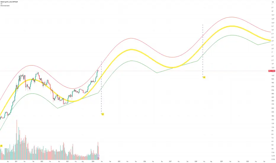
Bitcoin Market Cap wave model weeklyThis Bitcoin Market Cap wave model indicator is rooted in the foundation of my previously developed tool, the : Bitcoin wave model
To derive the Total Market Cap from the Bitcoin wave price model, I employed a straightforward estimation for the Total Market Supply (TMS). This estimation relies on the formula:
TMS <= (1 - 2^(-h)) for any h.This equation holds true for any value of h, which will be elaborated upon shortly. It is important to note that this inequality becomes the equality at the dates of halvings, diverging only slightly during other periods.
Bitcoin wave model is based on the logarithmic regression model and the sinusoidal waves, induced by the halving events.
This chart presents the outcome of an in-depth analysis of the complete set of Bitcoin price data available from October 2009 to August 2023.
The central concept is that the logarithm of the Bitcoin price closely adheres to the logarithmic regression model. If we plot the logarithm of the price against the logarithm of time, it forms a nearly straight line.
The parameters of this model are provided in the script as follows: log(BTCUSD) = 1.48 + 5.44log(h).
The secondary concept involves employing the inherent time unit of Bitcoin instead of days:
'h' denotes a slightly adjusted time measurement intrinsic to the Bitcoin blockchain. It can be approximated as (days since the genesis block) * 0.0007. Precisely, 'h' is defined as follows: h = 0 at the genesis block, h = 1 at the first halving block, and so forth. In general, h = block height / 210,000.
Adjustments are made to account for variations in block creation time.
The third concept revolves around investigating halving waves triggered by supply shock events resulting from the halvings. These halvings occur at regular intervals in Bitcoin's native time 'h'. All halvings transpire when 'h' is an integer. These events induce waves with intervals denoted as h = 1.
Consequently, we can model these waves using a sin(2pih - a) function. The parameter determining the time shift is assessed as 'a = 0.4', aligning with earlier expectations for halving events and their subsequent outcomes.
The fourth concept introduces the notion that the waves gradually diminish in amplitude over the progression of "time h," diminishing at a rate of 0.7^h.
Lastly, we can create bands around the modeled sinusoidal waves. The upper band is derived by multiplying the sine wave by a factor of 3.1*(1-0.16)^h, while the lower band is obtained by dividing the sine wave by the same factor, 3.1*(1-0.16)^h.
The current bandwidth is 2.5x. That means that the upper band is 2.5 times the lower band. These bands are forming an exceptionally narrow predictive channel for Bitcoin. Consequently, a highly accurate estimation of the peak of the next cycle can be derived.
The prediction indicates that the zenith past the fourth halving, expected around the summer of 2025, could result in Total Bitcoin Market Cap ranging between 4B and 5B USD.
The projections to the future works well only for weekly timeframe.
Enjoy the mathematical insights!
Bitcoin wave modelBitcoin wave model is based on the logarithmic regression model and the sinusoidal waves, induced by the halving events.
This chart presents the outcome of an in-depth analysis of the complete set of Bitcoin price data available from October 2009 to August 2023.
The central concept is that the logarithm of the Bitcoin price closely adheres to the logarithmic regression model. If we plot the logarithm of the price against the logarithm of time, it forms a nearly straight line.
The parameters of this model are provided in the script as follows: log (BTCUSD) = 1.48 + 5.44log(h).
The secondary concept involves employing the inherent time unit of Bitcoin instead of days:
'h' denotes a slightly adjusted time measurement intrinsic to the Bitcoin blockchain. It can be approximated as (days since the genesis block) * 0.0007. Precisely, 'h' is defined as follows: h = 0 at the genesis block, h = 1 at the first halving block, and so forth. In general, h = block height / 210,000.
Adjustments are made to account for variations in block creation time.
The third concept revolves around investigating halving waves triggered by supply shock events resulting from the halvings. These halvings occur at regular intervals in Bitcoin's native time 'h'. All halvings transpire when 'h' is an integer. These events induce waves with intervals denoted as h = 1.
Consequently, we can model these waves using a sin(2pih - a) function. The parameter determining the time shift is assessed as 'a = 0.4', aligning with earlier expectations for halving events and their subsequent outcomes.
The fourth concept introduces the notion that the waves gradually diminish in amplitude over the progression of "time h," diminishing at a rate of 0.7^h.
Lastly, we can create bands around the modeled sinusoidal waves. The upper band is derived by multiplying the sine wave by a factor of 3.1*(1-0.16)^h, while the lower band is obtained by dividing the sine wave by the same factor, 3.1*(1-0.16)^h.
The current bandwidth is 2.5x. That means that the upper band is 2.5 times the lower band. These bands are forming an exceptionally narrow predictive channel for Bitcoin. Consequently, a highly accurate estimation of the peak of the next cycle can be derived.
The prediction indicates that the zenith past the fourth halving, expected around the summer of 2025, could result in prices ranging between 200,000 and 240,000 USD.
Enjoy the mathematical insights!