N-Degree Moment-Based Adaptive Detection🙏🏻 N-Degree Moment-Based Adaptive Detection (NDMBAD) method is a generalization of MBAD since the horizontal line fit passing through the data's mean can be simply treated as zero-degree polynomial regression. We can extend the MBAD logic to higher-degree polynomial regression.
I don't think I need to talk a lot about the thing there; the logic is really the same as in MBAD, just hit the link above and read if you want. The only difference is now we can gather cumulants not only from the horizontal mean fit (degree = 0) but also from higher-order polynomial regression fit, including linear regression (degree = 1).
Why?
Simply because residuals from the 0-degree model don't contain trend information, and while in some cases that's exactly what you need, in other cases, you want to model your trend explicitly. Imagine your underlying process trends in a steady manner, and you want to control the extreme deviations from the process's core. If you're going to use 0-degree, you'll be treating this beautiful steady trend as a residual itself, which "constantly deviates from the process mean." It doesn't make much sense.
How?
First, if you set the length to 0, you will end up with the function incrementally applied to all your data starting from bar_index 0. This can be called the expanding window mode. That's the functionality I include in all my scripts lately (where it makes sense). As I said in the MBAD description, choosing length is a matter of doing business & applied use of my work, but I think I'm open to talk about it.
I don't see much sense in using degree > 1 though (still in research on it). If you have dem curves, you can use Fourier transform -> spectral filtering / harmonic regression (regression with Fourier terms). The job of a degree > 0 is to model the direction in data, and degree 1 gets it done. In mean reversion strategies, it means that you don't wanna put 0-degree polynomial regression (i.e., the mean) on non-stationary trending data in moving window mode because, this way, your residuals will be contaminated with the trend component.
By the way, you can send thanks to @aaron294c , he said like mane MBAD is dope, and it's gonna really complement his work, so I decided to drop NDMBAD now, gonna be more useful since it covers more types of data.
I wanned to call it N-Order Moment Adaptive Detection because it abbreviates to NOMAD, which sounds cool and suits me well, because when I perform as a fire dancer, nomad style is one of my outfits. Burning Man stuff vibe, you know. But the problem is degree and order really mean two different things in the polynomial context, so gotta stay right & precise—that's the priority.
∞
Moments

Moment-Based Adaptive DetectionMBAD (Moment-Based Adaptive Detection) : a method applicable to a wide range of purposes, like outlier or novelty detection, that requires building a sensible interval/set of thresholds. Unlike other methods that are static and rely on optimizations that inevitably lead to underfitting/overfitting, it dynamically adapts to your data distribution without any optimizations, MLE, or stuff, and provides a set of data-driven adaptive thresholds, based on closed-form solution with O(n) algo complexity.
1.5 years ago, when I was still living in Versailles at my friend's house not knowing what was gonna happen in my life tomorrow, I made a damn right decision not to give up on one idea and to actually R&D it and see what’s up. It allowed me to create this one.
The Method Explained
I’ve been wandering about z-values, why exactly 6 sigmas, why 95%? Who decided that? Why would you supersede your opinion on data? Based on what? Your ego?
Then I consciously noticed a couple of things:
1) In control theory & anomaly detection, the popular threshold is 3 sigmas (yet nobody can firmly say why xD). If your data is Laplace, 3 sigmas is not enough; you’re gonna catch too many values, so it needs a higher sigma.
2) Yet strangely, the normal distribution has kurtosis of 3, and 6 for Laplace.
3) Kurtosis is a standardized moment, a moment scaled by stdev, so it means "X amount of something measured in stdevs."
4) You generate synthetic data, you check on real data (market data in my case, I am a quant after all), and you see on both that:
lower extension = mean - standard deviation * kurtosis ≈ data minimum
upper extension = mean + standard deviation * kurtosis ≈ data maximum
Why not simply use max/min?
- Lower info gain: We're not using all info available in all data points to estimate max/min; we just pick the current higher and lower values. Lol, it’s the same as dropping exponential smoothing with alpha = 0 on stationary data & calling it a day.
You can’t update the estimates of min and max when new data arrives containing info about the matter. All you can do is just extend min and max horizontally, so you're not using new info arriving inside new data.
- Mixing order and non-order statistics is a bad idea; we're losing integrity and coherence. That's why I don't like the Hurst exponent btw (and yes, I came up with better metrics of my own).
- Max & min are not even true order statistics, unlike a percentile (finding which requires sorting, which requires multiple passes over your data). To find min or max, you just need to do one traversal over your data. Then with or without any weighting, 100th percentile will equal max. So unlike a weighted percentile, you can’t do weighted max. Then while you can always check max and min of a geometric shape, now try to calculate the 56th percentile of a pentagram hehe.
TL;DR max & min are rather topological characteristics of data, just as the difference between starting and ending points. Not much to do with statistics.
Now the second part of the ballet is to work with data asymmetry:
1) Skewness is also scaled by stdev -> so it must represent a shift from the data midrange measured in stdevs -> given asymmetric data, we can include this info in our models. Unlike kurtosis, skewness has a sign, so we add it to both thresholds:
lower extension = mean - standard deviation * kurtosis + standard deviation * skewness
upper extension = mean + standard deviation * kurtosis + standard deviation * skewness
2) Now our method will work with skewed data as well, omg, ain’t it cool?
3) Hold up, but what about 5th and 6th moments (hyperskewness & hyperkurtosis)? They should represent something meaningful as well.
4) Perhaps if extensions represent current estimated extremums, what goes beyond? Limits, beyond which we expect data not to be able to pass given the current underlying process generating the data?
When you extend this logic to higher-order moments, i.e., hyperskewness & hyperkurtosis (5th and 6th moments), they measure asymmetry and shape of distribution tails, not its core as previous moments -> makes no sense to mix 4th and 3rd moments (skewness and kurtosis) with 5th & 6th, so we get:
lower limit = mean - standard deviation * hyperkurtosis + standard deviation * hyperskewness
upper limit = mean + standard deviation * hyperkurtosis + standard deviation * hyperskewness
While extensions model your data’s natural extremums based on current info residing in the data without relying on order statistics, limits model your data's maximum possible and minimum possible values based on current info residing in your data. If a new data point trespasses limits, it means that a significant change in the data-generating process has happened, for sure, not probably—a confirmed structural break.
And finally we use time and volume weighting to include order & process intensity information in our model.
I can't stress it enough: despite the popularity of these non-weighted methods applied in mainstream open-access time series modeling, it doesn’t make ANY sense to use non-weighted calculations on time series data . Time = sequence, it matters. If you reverse your time series horizontally, your means, percentiles, whatever, will stay the same. Basically, your calculations will give the same results on different data. When you do it, you disregard the order of data that does have order naturally. Does it make any sense to you? It also concerns regressions applied on time series as well, because even despite the slope being opposite on your reversed data, the centroid (through which your regression line always comes through) will be the same. It also might concern Fourier (yes, you can do weighted Fourier) and even MA and AR models—might, because I ain’t researched it extensively yet.
I still can’t believe it’s nowhere online in open access. No chance I’m the first one who got it. It’s literally in front of everyone’s eyes for centuries—why no one tells about it?
How to use
That’s easy: can be applied to any, even non-stationary and/or heteroscedastic time series to automatically detect novelties, outliers, anomalies, structural breaks, etc. In terms of quant trading, you can try using extensions for mean reversion trades and limits for emergency exits, for example. The market-making application is kinda obvious as well.
The only parameter the model has is length, and it should NOT be optimized but picked consciously based on the process/system you’re applying it to and based on the task. However, this part is not about sharing info & an open-access instrument with the world. This is about using dem instruments to do actual business, and we can’t talk about it.
∞

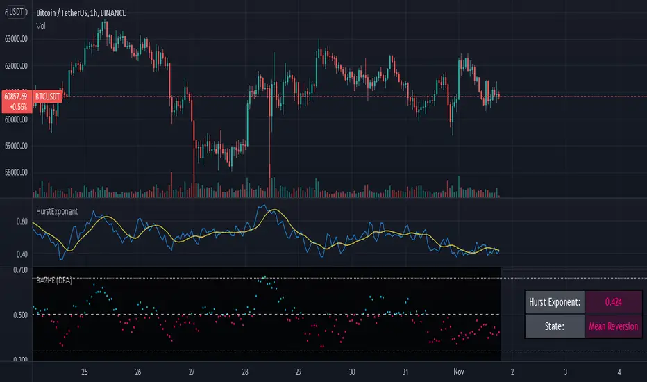
HurstExponentLibrary "HurstExponent"
Library to calculate Hurst Exponent refactored from Hurst Exponent - Detrended Fluctuation Analysis
demean(src) Calculates a series subtracted from the series mean.
Parameters:
src : The series used to calculate the difference from the mean (e.g. log returns).
Returns: The series subtracted from the series mean
cumsum(src, length) Calculates a cumulated sum from the series.
Parameters:
src : The series used to calculate the cumulative sum (e.g. demeaned log returns).
length : The length used to calculate the cumulative sum (e.g. 100).
Returns: The cumulative sum of the series as an array
aproximateLogScale(scale, length) Calculates an aproximated log scale. Used to save sample size
Parameters:
scale : The scale to aproximate.
length : The length used to aproximate the expected scale.
Returns: The aproximated log scale of the value
rootMeanSum(cumulativeSum, barId, numberOfSegments) Calculates linear trend to determine error between linear trend and cumulative sum
Parameters:
cumulativeSum : The cumulative sum array to regress.
barId : The barId for the slice
numberOfSegments : The total number of segments used for the regression calculation
Returns: The error between linear trend and cumulative sum
averageRootMeanSum(cumulativeSum, barId, length) Calculates the Root Mean Sum Measured for each block (e.g the aproximated log scale)
Parameters:
cumulativeSum : The cumulative sum array to regress and determine the average of.
barId : The barId for the slice
length : The length used for finding the average
Returns: The average root mean sum error of the cumulativeSum
criticalValues(length) Calculates the critical values for a hurst exponent for a given length
Parameters:
length : The length used for finding the average
Returns: The critical value, upper critical value and lower critical value for a hurst exponent
slope(cumulativeSum, length) Calculates the hurst exponent slope measured from root mean sum, scaled to log log plot using linear regression
Parameters:
cumulativeSum : The cumulative sum array to regress and determine the average of.
length : The length used for the hurst exponent sample size
Returns: The slope of the hurst exponent
smooth(src, length) Smooths input using advanced linear regression
Parameters:
src : The series to smooth (e.g. hurst exponent slope)
length : The length used to smooth
Returns: The src smoothed according to the given length
exponent(src, hurstLength) Wrapper function to calculate the hurst exponent slope
Parameters:
src : The series used for returns calculation (e.g. close)
hurstLength : The length used to calculate the hurst exponent (should be greater than 50)
Returns: The src smoothed according to the given length
MomentsLibrary "Moments"
Based on Moments (Mean,Variance,Skewness,Kurtosis) . Rewritten for Pinescript v5.
logReturns(src) Calculates log returns of a series (e.g log percentage change)
Parameters:
src : Source to use for the returns calculation (e.g. close).
Returns: Log percentage returns of a series
mean(src, length) Calculates the mean of a series using ta.sma
Parameters:
src : Source to use for the mean calculation (e.g. close).
length : Length to use mean calculation (e.g. 14).
Returns: The sma of the source over the length provided.
variance(src, length) Calculates the variance of a series
Parameters:
src : Source to use for the variance calculation (e.g. close).
length : Length to use for the variance calculation (e.g. 14).
Returns: The variance of the source over the length provided.
standardDeviation(src, length) Calculates the standard deviation of a series
Parameters:
src : Source to use for the standard deviation calculation (e.g. close).
length : Length to use for the standard deviation calculation (e.g. 14).
Returns: The standard deviation of the source over the length provided.
skewness(src, length) Calculates the skewness of a series
Parameters:
src : Source to use for the skewness calculation (e.g. close).
length : Length to use for the skewness calculation (e.g. 14).
Returns: The skewness of the source over the length provided.
kurtosis(src, length) Calculates the kurtosis of a series
Parameters:
src : Source to use for the kurtosis calculation (e.g. close).
length : Length to use for the kurtosis calculation (e.g. 14).
Returns: The kurtosis of the source over the length provided.
skewnessStandardError(sampleSize) Estimates the standard error of skewness based on sample size
Parameters:
sampleSize : The number of samples used for calculating standard error.
Returns: The standard error estimate for skewness based on the sample size provided.
kurtosisStandardError(sampleSize) Estimates the standard error of kurtosis based on sample size
Parameters:
sampleSize : The number of samples used for calculating standard error.
Returns: The standard error estimate for kurtosis based on the sample size provided.
skewnessCriticalValue(sampleSize) Estimates the critical value of skewness based on sample size
Parameters:
sampleSize : The number of samples used for calculating critical value.
Returns: The critical value estimate for skewness based on the sample size provided.
kurtosisCriticalValue(sampleSize) Estimates the critical value of kurtosis based on sample size
Parameters:
sampleSize : The number of samples used for calculating critical value.
Returns: The critical value estimate for kurtosis based on the sample size provided.
