Volume Analysis - Heatmap and Volume ProfileHello All!
I have a new toy for you! Volume Analysis - Heatmap and Volume Profile . Honestly I started to work to develop Volume Heatmap then I decided to improve it and add more features such Volume profile, volume, difference in Buy/Sell volumes etc. I tried to put my abilities into this script and tried to use some new Pine Language™ features ( method, force_overlay, enum etc features ). I hope the usage of these new features would be an example for Pine Programmers.
Lets talk about how it works:
- It gets number of Rows/Columns from the user for each candle to create heatmap
- It calculates the number of the candles to analyze. Number of the candles may change by number of Rows/columns or if any volume / difference in volumes / volume profile is enabled
- It gets Closing/Opening price, Volume and Time info from lower time frame for each candle ( it can be up to 100K for each candle )
- After getting the data it calculates lower time frame to analyze
- Then it calculates how closing price moves, how much volume on each move and create boxes by the volume/move in each box
- The colors for each box calculated by volume info and closing price movements in the lower time frame
- It shows the boxes on Absolute places or Zero Line optionally
- it shows Volume, Cumulative volume, Difference between Buy/Sell volume for each column
- it changes empty box color by Chart background color, also you can change transparency
- At this time it creates Volume Profile with up to 25 rows
- As a new Pine Language™ feature, it can show Volume Profile in the indicator window or in Main chart, shows Value Area, Value Area High (VAH), Value Area Low (VAL), and draw it and POC (Point Of Control) in the indicator window and/or in the main chart
- Honestly the feature I like is that: For the markets that are not open 24/7, it combines the data from the lower time period without any gaps. For example, if you work for a market that is closed on Saturdays and Sundays, it ensures data integrity by omitting weekends and holidays. so for example if the data is like "ABC---DEF-X---YL-Z" then it makes this data like "ABCDEFXYLZ". In this way, there will be no data breaks in the displayed boxes, there will be no empty colons, and it will appear as if data is coming in at any time.
- Finally it shows Info Panel to give info, its background color automatically changes by the Chart background color
- Important! You should set your "Plan" accordingly, your plan is "Premium or Higher" or "Lower tier". so the script can understand the minimum time frame it can get data!!
I tried to share many screenshots below to explain it much better
How it looks?
it shows Highest Buy/Sell volumes brighter, move volume -> brighter
Volume Profile ( up to 25 row s) ( number of contained candles should be more than 1 )
Volume Profile can be shown in the main chart optionally
How the main chart looks:
Closing price shown and you can enable it, change colors & line width
Can include many candles according to Row&Column number you set
Optionally it can show cumulative volume for each candle
Closing prices from lower time frame
Shows Candle Body by changing background colors
It can shows all included candles on Zero line
You can change the colors of many things
You can set Empty box and border transparency
Table, Empty box Colors adjustment done automatically by chart background color
Sometimes we can not get data from some historical candles if time frame is high such 2days, 1 week etc, and it looks like:
It also checks if Chart time frame and Chart type is suitable
Enjoy!
Cerca negli script per " TABLE"

Intermarket Correlation TableThe Correlation Coefficient is used to measure the correlation between two sets of data. In the trading world, the Correlation Coefficient is a measure of the correlation between two data sets of financial instruments. The correlation between two financial instruments is the degree in which they are related. Correlation is based on a scale of 1 to -1. The closer the Correlation Coefficient is to 1, the higher their positive correlation. The instruments will move up and down together. The closer the Correlation coefficient is to -1, the more they move in opposite directions. A value at 0 indicates that there is no correlation.
This indicator uses the built in ta.correlation function to calculate the correlation coefficient between DXY and NQ, ES, YM, US10Y, and ZN respectively. It then presents the data in a customizable table that is view as an overlay on your chart.
Adjust the length of the correlation factor to calculate higher time frame correlation.
Asset background changes based on current candle direction.
Coefficient background color changes based on whether the assets are properly correlated.
DXY is inversely correlated to NQ, ES, YM, and ZN.
DXY is directly correlated to US10Y.
The colors are reflected as such.

Volatility DashboardThis indicator calculates and displays volatility metrics for a specified number of bars (rolling window) on a TradingView chart. It can be customized to display information in English or Thai and can position the dashboard at various locations on the chart.
Inputs
Language: Users can choose between English ("ENG") and Thai ("TH") for the dashboard's language.
Dashboard Position: Users can specify where the dashboard should appear on the chart. Options include various positions such as "Bottom Right", "Top Center", etc.
Calculation Method: Currently, the script supports "High-Low" for volatility calculation. This method calculates the difference between the highest and lowest prices within a specified timeframe.
Bars: Number of bars used to calculate the volatility.
Display Logic
Fills the islast_vol_points array with the calculated volatility points.
Sets the table cells with headers and corresponding values:
=> Highest Volatility: The maximum value in the islast_vol_points array
=> Mean Volatility: The average value in the islast_vol_points array,
=> Lowest Volatility: The minimum value in the islast_vol_points array, Number of Bars: The rolling window size.

Futures Tick and Point Value TableDisplays a table in the upper right corner of the chart showing the tick and point value in USD.

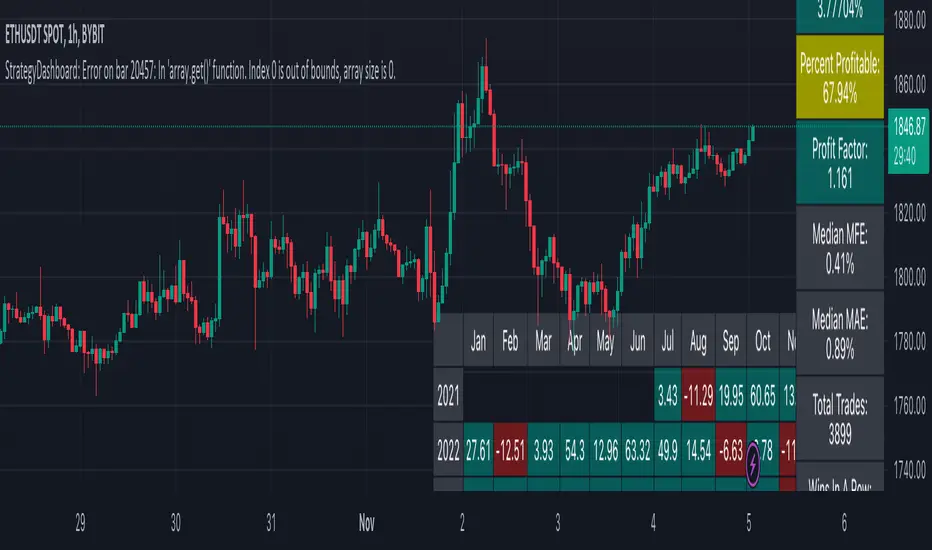
StrategyDashboardLibrary ”StrategyDashboard”
Hey, everybody!
I haven’t done anything here for a long time, I need to get better ^^.
In my strategies, so far private, but not about that, I constantly use dashboards, which clearly show how my strategy is working out.
Of course, you can also find a number of these parameters in the standard strategy window, but I prefer to display everything on the screen, rather than digging through a bunch of boxes and dropdowns.
At the moment I am using 2 dashboards, which I would like to share with you.
1. monthly(isShow)
this is a dashboard with the breakdown of profit by month in per cent. That is, it displays how much percentage you made or lost in a particular month, as well as for the year as a whole.
Parameters:
isShow (bool) - determine allowance to display or not.
2. total(isShow)
The second dashboard displays more of the standard strategy information, but in a table format. Information from the series “number of consecutive losers, number of consecutive wins, amount of earnings per day, etc.”.
Parameters:
isShow (bool) - determine allowance to display or not.
Since I prefer the dark theme of the interface, now they are adapted to it, but in the near future for general convenience I will add the ability to adapt to light.
The same goes for the colour scheme, now it is adapted to the one I use in my strategies (because the library with more is made by cutting these dashboards from my strategies), but will also make customisable part.
If you have any wishes, feel free to write in the comments, maybe I can implement and add them in the next versions.
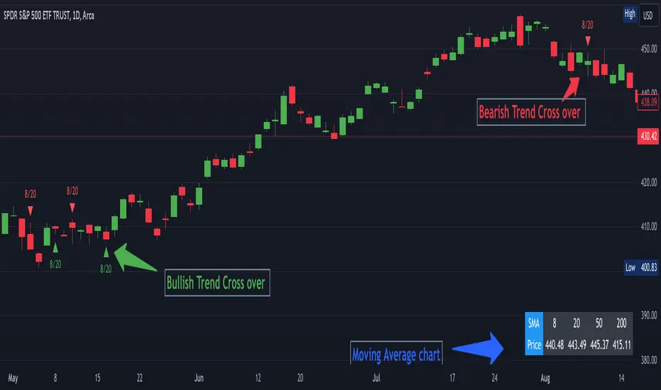
SMA Table with Alerts and Intersections🌟 **Presenting the Dynamic SMA Intersection Alert Indicator!** 🌟
### **Overview:**
The Dynamic SMA Intersection Alert Indicator is a sophisticated tool developed for traders seeking simplicity and effectiveness. It integrates multiple Simple Moving Averages (SMA) to deliver real-time alerts and visual cues, enabling traders to identify potential market entry points with ease.
### **Features:**
1. **Multi-SMA Visualization:**
- Incorporates four SMAs: 8, 20, 50, 200 periods.
- Displays a customizable table showing the current value of each SMA.
2. **Alerts in Real-Time:**
- Provides instant notifications for price crossings over any of the SMAs.
- Offers customizable alert messages.
3. **Visualization of Intersection Points:**
- Displays green triangles for bullish crosses and red for bearish, directly on the chart.
- Allows for the identification of precise intersection points between shorter-term and longer-term SMAs.
### **Benefits:**
- **Informed Decision-Making:** Enables quick discernment of market trends.
- **Efficiency:** Automates the tracking of SMA intersections.
- **User-Friendly:** Applicable for both novice and experienced traders.
### **How It Operates:**
- The indicator computes four different SMAs and presents their current values systematically.
- It triggers a real-time alert when the price crosses any SMA, instantly notifying the trader.
- Visual cues are plotted on the chart when any two SMAs intersect, indicating the type of cross.
### **Enhance Your Trading Experience!**
The Dynamic SMA Intersection Alert Indicator is designed to refine your trading experience and assist in making informed and timely trading decisions. Leverage this tool to stay abreast of market trends and enhance your market understanding!
AL-Ghamdi Table Harmonic
AL-Ghamdi Table Harmonic
A simple note showing the proportions of the harmonic models
With correction, target and stop loss

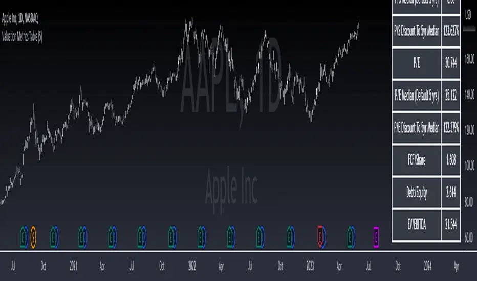
Valuation Metrics Table (P/S, P/E, etc.)This table gives the user a very easy way of seeing many valuation metrics. I also included the 5 year median of the price to sales and price to earnings ratios. Then I calculated the percent difference between the median and the current ratio. This gives a sense of whether or not a stock is over valued or under valued based on historical data. The other ratios are well known and don't require any explanation. You can turn off the ones you don't want in the settings of the indicator. Another thing to mention is that diluted EPS is used in calculations
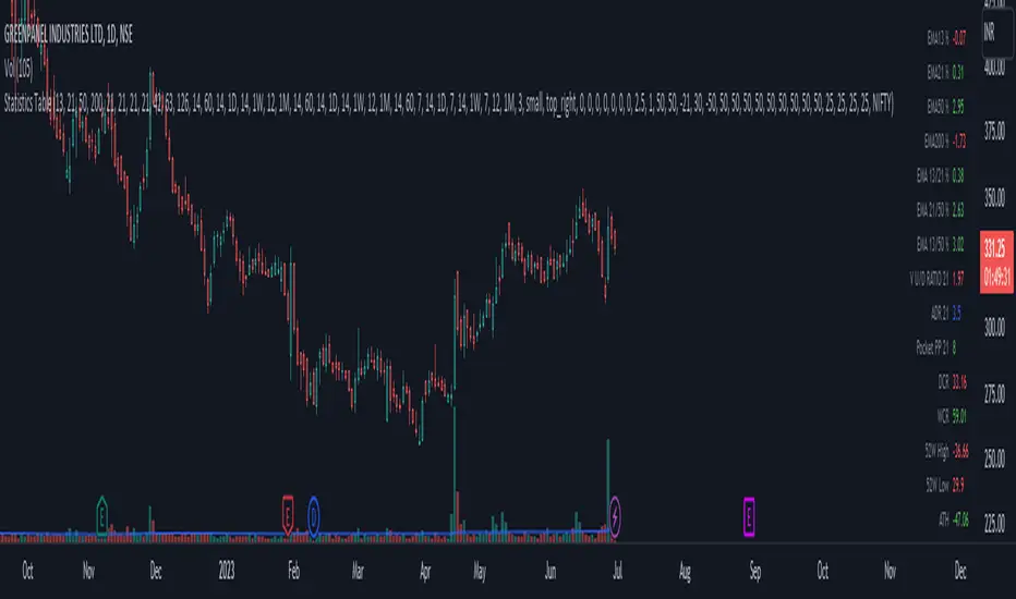
Statistics TableThis script display some useful Statistics data that can be useful in making trading decision.
Here the list of information this script is display in table format.
You can change each and every single ema and rs length as per your need from setting.
1) close difference from first ema
2) close difference from second ema
3) close difference from third ema
4) close difference from fourth ema
5) difference between first and second ema
6) difference between second and third ema
7) difference between first and third ema
8) volume up down ratio
9) ATR/ADR %
10) volume pocket pivot count
11) daily closing range
12) weekly closing range
13) close difference from 52week high
14) close difference from 52week low
15) close difference from All time high
16) close difference from All time low
17) rs line above or below first rs ema
18) rs line above or below second rs ema
19) rs line above or below third rs ema
20) rs line above or below fourth rs ema
21) first rs value
22) second rs value
23) third rs value
24) fourth rs value
25) difference between previous first rs length days change % and current first rs length days change %
26) difference between previous second rs length days change % and current second rs length days change %
27) difference between previous third rs length days change % and current third rs length days change %
Astro: Planetary Aspect TableIn astrology, planetary aspects refer to the angles formed between two or more planets in a horoscope or birth chart. These angles are created by the positions of the planets in the sky and are thought to represent a particular energy or influence that can impact events on Earth.
The most common planetary aspects are the conjunction (when two planets are in the same position in the zodiac), the opposition (when two planets are direct across from each other in the zodiac), the trine (when two planets are 120 degrees apart in the zodiac), and the square (when two planets are 90 degrees apart in the zodiac).
This chart overlay displays a real-time table of current interplanetary aspects for all AstroLib celestial body combinations.

[-_-] 2D FractalsThe sole purpose of this script is to demonstrate what's possible to make with Pinescript, namely to display images (2D Fractals in this case).
The script consists of two functions: one that generates the values of a fractal and one that displays them (utilising table) with each cell being used as a "pixel". We can control the "resolution" of image, as well as choose one of three fractal types.

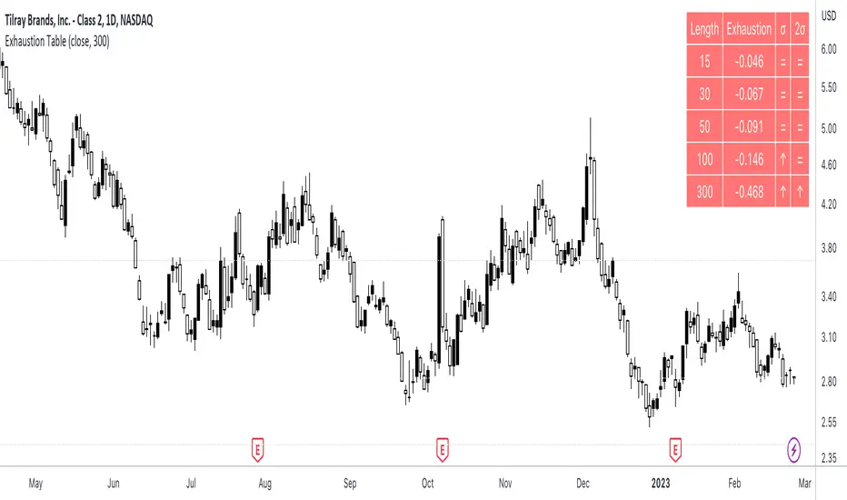
Exhaustion Table [SpiritualHealer117]A simple indicator in a table format, is effective for determining when an individual stock or cryptocurrency is oversold or overbought.
Using the indicator
In the column "2σ" , up arrows indicate that the asset is very overbought , down arrows indicate that an asset is very oversold , and an equals sign indicates that the indicator is neutral.
In the column "σ" , up arrows indicate that the asset is overbought , down arrows indicate that an asset is oversold , and an equals sign indicates that the indicator is neutral.
What indicator is
The indicator shows the exhaustion (percentage gap between the closing price and a moving average) at 5 given lengths, 15, 30, 50, 100, and 300. It compares that to two thresholds for exhaustion: one standard deviation out and one two standard deviations out.
Multi indicators tableThis is a comprehensive trading tool that presents an overview of the market in a tabular format. It consists of five distinct categories of trading indicators : Volatility, Trend, Momentum, Reversal, and Volume. Each category includes a series of indicators that are widely used in the trading communauty.
The Volatility category includes the Average True Range (ATR) and Bollinger Bands indicators. The Trend category comprises the Average Directional Index (ADX), four Exponential Moving Averages (EMAs), Aroon, Parabolic SAR, and the Supertrend. The Momentum category includes the Stochastic Relative Strength Index (StochRSI), Money Flow Index (MFI), Williams %R, Relative Strength Index (RSI), and Commodity Channel Index (CCI). The Reversal category includes Parabolic SAR, Moving Average Convergence Divergence (MACD), and PP Supertrend. Finally, the Volume category includes the Volume Exponential Moving Average (EMA) indicator.
The indicators states are easily readable, the indicator case is colored based on his actual state. A bullish color (green by default), a bearish color (red by default),
a very bullish color (dark green by default), a very bearish color (dark red by default) and a neutral color (gray by default) displayed when the indicator doesn't give us a clear signal. Some indicators do not have a very bullish or very bearish state. Concerning volatility indicators, the bullish color indicates high volatility, the bearish color indicates low volatility, and the neutral color indicates normal volatility.
Most of the indicators displayed in the table are customizable, and traders can choose to hide the categories they don't want to use. The Indicator provides a quick and easily readable view on the market and allows traders to reduce the number of indicators on their chart making it lighter and more readable.

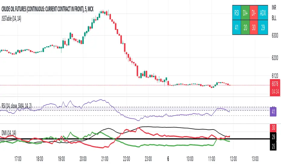
JSS Table - RSI, DI+, DI-, ADXSimple table to show the values for indicators which can be used to initiate trades:
RSI: Long above 55 // Short below 45 // Choppy between 45-55
DI+: Long above 25
DI-: Short above 25
Note when to avoid trend trades:
- If DI+ and DI- are both below 25 then market is choppy
- If RSI is between 45-55 then market is choppy
CFH | RSI-SRSI tableShows RSI and SRSI values on multiple timeframes, highlights oversold and overbought
Timeframes and colors are customizable
/V1llager/

Timeframe Bias TableAllows you to display a bias for the W, D, 4h, 15m & 1m Timeframes based on your own analysis.

TradingCube : Moving Average : Data tablePlots moving average both EMA as well as SMA on Multiple timeframes at once in a Tabular Format
for rapid indication of momentum shift as well as slower-moving confirmations.
Displays EMA/SMA 5 8, 13, 21,34,55,89,100,200,400 by default as well as provide the users the flexibility to choose the timeframe as per their set up.
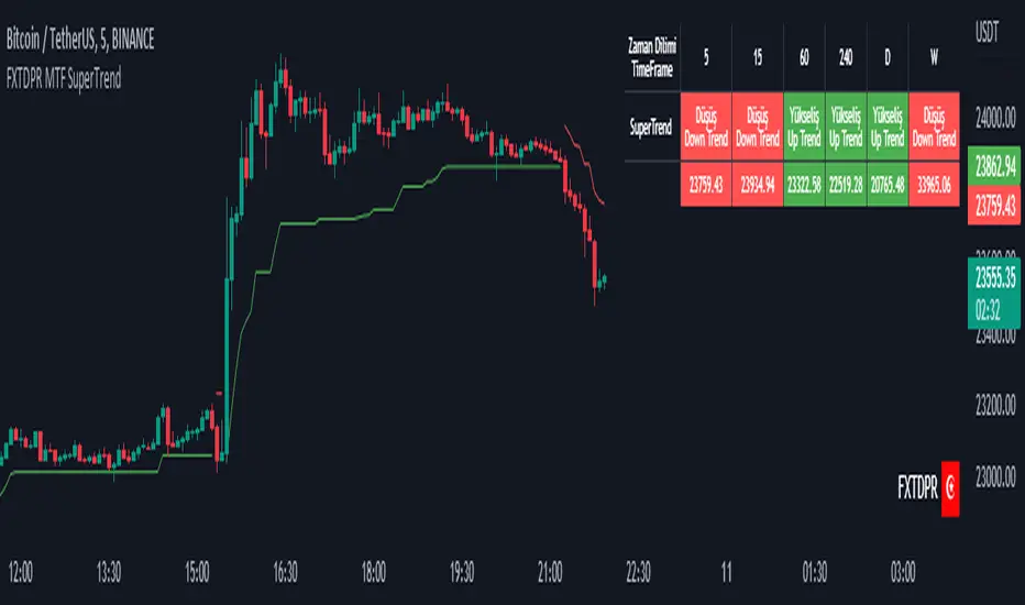
Mtf Supertrend Table
english
It is a study of how the supertrend indicator looks on multiple timeframes. You can see the Supertrend direction in Multiple Timeframes by looking at the chart
Türkçe
supertrend indikatörünün çoklu zaman dilimdlerinde nasıl göründüğü yönünde bir çalışmadır. Tabloya bakarak Çoklu Zaman dilimlerinde Supertrend yönünü görebilirsiniz
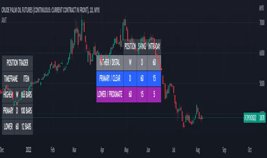
Alternative MTF Table█ OVERVIEW
This indicator is an educational indicator which was stripped down from Regression Channel Alternative MTF to display 3 timeframes based on timeframe scenarios.
The timeframe scenarios are defined based on Position, Swing and Intraday Trader.
█ INSPIRATION
It is possible to use array.new_bool, array.indexof and switch to get this outcome. Credits to TradingView .
Spinn ATR tableThe table contains summary data on the ATR from different timeframes and for different periods. You can view both absolute values and the percentage of the average price move to the current price.
This data can be used to compare the ATR on different timeframes. And, most importantly, you can compare the ATR of different coins.
In addition, the last column shows the average deviation of the ATR for each of the timeframes. You can compare these values on different coins to determine which ones are more volatile .
Note.
Using the indicator on different timeframes may give slightly different values due to the difference in the stored data for these timeframes.
--
В таблице собраны сводные данные по ATR с разных таймфреймов и за разные периоды. Можно просматривать как абсолютные значения, так и процентное соотношение среднего хода цены к текущей цене.
Эти данные можно использовать, чтобы сравнить ATR на разных таймфреймах. И, самое главное, можно сравнивать ATR разных монет.
Кроме того, в последней колонке указано среднее отклонение ATR по каждому из таймфреймов. Можно сравнивать эти значения на разных монетах, чтобы определить - какие из них более волатильны .
Примечание.
Использование индикатора на разных таймфреймах может давать слегка разные значения из-за разницы в хранимых данных для этих таймфреймов.


Multiple Indicator 50EMA Cross AlertsHere’s a screener including Symbol, Price, TSI, and 50 ema cross in a table output.
The 50 Exponential Moving Average is a trend indicator
You can find bullish momentum when the 50 ema crossed over or a bearish momentum when the 50 ema crossed under we are looking to take advantage by trading the reversion of these trends.
True strength index (TSI) is a trend momentum indicator
Readings are bullish when the True Strength Index shows positive values
Readings are bearish when the indicator displays negative values.
When a value is above 20, we look for selling overbought opportunity and when the value is under 20, we look for buying oversold opportunity.
You can select the pair of your choice in the settings.
Make sure to create an alert and choose any alerts then an alert will trigger when a price cross under or cross over the 50 ema for every pair separately.
This allow the user to verify if there is a trade set up or not.
Disclaimer
This post and the script don’t provide any financial advice.
Performance Table From OpenThis indicator plots the percentage performance from the open of up to 20 different customizable tickers.
Enjoy!
