EXODUS EXODUS by (DAFE) Trading Systems
EXODUS is a sophisticated trading algorithm built by Dskyz (DAFE) Trading Systems for competitive and competition purposes, designed to identify high-probability trades with robust risk management. this strategy leverages a multi-signal voting system, combining three core components—SPR, VWMO, and VEI—alongside ADX, choppiness filters, and ATR-based volatility gates to ensure trades are taken only in favorable market conditions. the algo uses a take-profit to stop-loss ratio, dynamic position sizing, and a strict voting mechanism requiring all signals to align before entering a trade.
EXODUS was not overfitted for any specific symbol. instead, it uses a generic tuned setting, making it versatile across various markets. while it can trade futures, it’s not currently set up for it but has the potential to do more with further development. visuals are intentionally minimal due to its competition focus, prioritizing performance over aesthetics. a more visually stunning version may be released in the future with enhanced graphics.
The Unique Core Components Developed for EXODUS
SPR (Session Price Recalibration)
SPR measures momentum during regular trading hours (RTH, 0930-1600, America/New_York) to catch session-specific trends.
spr_lookback = input.int(15, "SPR Lookback") this sets how many bars back SPR looks to calculate momentum (default 15 bars). it compares the current session’s price-volume score to the score 15 bars ago to gauge momentum strength.
how it works: a longer lookback smooths out the signal, focusing on bigger trends. a shorter one makes SPR more sensitive to recent moves.
how to adjust: on a 1-hour chart, 15 bars is 15 hours (about 2 trading days). if you’re on a shorter timeframe like 5 minutes, 15 bars is just 75 minutes, so you might want to increase it to 50 or 100 to capture more meaningful trends. if you’re trading a choppy stock, a shorter lookback (like 5) can help catch quick moves, but it might give more false signals.
spr_threshold = input.float (0.7, "SPR Threshold")
this is the cutoff for SPR to vote for a trade (default 0.7). if SPR’s normalized value is above 0.7, it votes for a long; below -0.7, it votes for a short.
how it works: SPR normalizes its momentum score by ATR, so this threshold ensures only strong moves count. a higher threshold means fewer trades but higher conviction.
how to adjust: if you’re getting too few trades, lower it to 0.5 to let more signals through. if you’re seeing too many false entries, raise it to 1.0 for stricter filtering. test on your chart to find a balance.
spr_atr_length = input.int(21, "SPR ATR Length") this sets the ATR period (default 21 bars) used to normalize SPR’s momentum score. ATR measures volatility, so this makes SPR’s signal relative to market conditions.
how it works: a longer ATR period (like 21) smooths out volatility, making SPR less jumpy. a shorter one makes it more reactive.
how to adjust: if you’re trading a volatile stock like TSLA, a longer period (30 or 50) can help avoid noise. for a calmer stock, try 10 to make SPR more responsive. match this to your timeframe—shorter timeframes might need a shorter ATR.
rth_session = input.session("0930-1600","SPR: RTH Sess.") rth_timezone = "America/New_York" this defines the session SPR uses (0930-1600, New York time). SPR only calculates momentum during these hours to focus on RTH activity.
how it works: it ignores pre-market or after-hours noise, ensuring SPR captures the main market action.
how to adjust: if you trade a different session (like London hours, 0300-1200 EST), change the session to match. you can also adjust the timezone if you’re in a different region, like "Europe/London". just make sure your chart’s timezone aligns with this setting.
VWMO (Volume-Weighted Momentum Oscillator)
VWMO measures momentum weighted by volume to spot sustained, high-conviction moves.
vwmo_momlen = input.int(21, "VWMO Momentum Length") this sets how many bars back VWMO looks to calculate price momentum (default 21 bars). it takes the price change (close minus close 21 bars ago).
how it works: a longer period captures bigger trends, while a shorter one reacts to recent swings.
how to adjust: on a daily chart, 21 bars is about a month—good for trend trading. on a 5-minute chart, it’s just 105 minutes, so you might bump it to 50 or 100 for more meaningful moves. if you want faster signals, drop it to 10, but expect more noise.
vwmo_volback = input.int(30, "VWMO Volume Lookback") this sets the period for calculating average volume (default 30 bars). VWMO weights momentum by volume divided by this average.
how it works: it compares current volume to the average to see if a move has strong participation. a longer lookback smooths the average, while a shorter one makes it more sensitive.
how to adjust: for stocks with spiky volume (like NVDA on earnings), a longer lookback (50 or 100) avoids overreacting to one-off spikes. for steady volume stocks, try 20. match this to your timeframe—shorter timeframes might need a shorter lookback.
vwmo_smooth = input.int(9, "VWMO Smoothing")
this sets the SMA period to smooth VWMO’s raw momentum (default 9 bars).
how it works: smoothing reduces noise in the signal, making VWMO more reliable for voting. a longer smoothing period cuts more noise but adds lag.
how to adjust: if VWMO is too jumpy (lots of false votes), increase to 15. if it’s too slow and missing trades, drop to 5. test on your chart to see what keeps the signal clean but responsive.
vwmo_threshold = input.float(10, "VWMO Threshold") this is the cutoff for VWMO to vote for a trade (default 10). above 10, it votes for a long; below -10, a short.
how it works: it ensures only strong momentum signals count. a higher threshold means fewer but stronger trades.
how to adjust: if you want more trades, lower it to 5. if you’re getting too many weak signals, raise it to 15. this depends on your market—volatile stocks might need a higher threshold to filter noise.
VEI (Velocity Efficiency Index)
VEI measures market efficiency and velocity to filter out choppy moves and focus on strong trends.
vei_eflen = input.int(14, "VEI Efficiency Smoothing") this sets the EMA period for smoothing VEI’s efficiency calc (bar range / volume, default 14 bars).
how it works: efficiency is how much price moves per unit of volume. smoothing it with an EMA reduces noise, focusing on consistent efficiency. a longer period smooths more but adds lag.
how to adjust: for choppy markets, increase to 20 to filter out noise. for faster markets, drop to 10 for quicker signals. this should match your timeframe—shorter timeframes might need a shorter period.
vei_momlen = input.int(8, "VEI Momentum Length") this sets how many bars back VEI looks to calculate momentum in efficiency (default 8 bars).
how it works: it measures the change in smoothed efficiency over 8 bars, then adjusts for inertia (volume-to-range). a longer period captures bigger shifts, while a shorter one reacts faster.
how to adjust: if VEI is missing quick reversals, drop to 5. if it’s too noisy, raise to 12. test on your chart to see what catches the right moves without too many false signals.
vei_threshold = input.float(4.5, "VEI Threshold") this is the cutoff for VEI to vote for a trade (default 4.5). above 4.5, it votes for a long; below -4.5, a short.
how it works: it ensures only strong, efficient moves count. a higher threshold means fewer trades but higher quality.
how to adjust: if you’re not getting enough trades, lower to 3. if you’re seeing too many false entries, raise to 6. this depends on your market—fast stocks like NQ1 might need a lower threshold.
Features
Multi-Signal Voting: requires all three signals (SPR, VWMO, VEI) to align for a trade, ensuring high-probability setups.
Risk Management: uses ATR-based stops (2.1x) and take-profits (4.1x), with dynamic position sizing based on a risk percentage (default 0.4%).
Market Filters: ADX (default 27) ensures trending conditions, choppiness index (default 54.5) avoids sideways markets, and ATR expansion (default 1.12) confirms volatility.
Dashboard: provides real-time stats like SPR, VWMO, VEI values, net P/L, win rate, and streak, with a clean, functional design.
Visuals
EXODUS prioritizes performance over visuals, as it was built for competitive and competition purposes. entry/exit signals are marked with simple labels and shapes, and a basic heatmap highlights market regimes. a more visually stunning update may be released later, with enhanced graphics and overlays.
Usage
EXODUS is designed for stocks and ETFs but can be adapted for futures with adjustments. it performs best in trending markets with sufficient volatility, as confirmed by its generic tuning across symbols like TSLA, AMD, NVDA, and NQ1. adjust inputs like SPR threshold, VWMO smoothing, or VEI momentum length to suit specific assets or timeframes.
Setting I used: (Again, these are a generic setting, each security needs to be fine tuned)
SPR LB = 19 SPR TH = 0.5 SPR ATR L= 21 SPR RTH Sess: 9:30 – 16:00
VWMO L = 21 VWMO LB = 18 VWMO S = 6 VWMO T = 8
VEI ES = 14 VEI ML = 21 VEI T = 4
R % = 0.4
ATR L = 21 ATR M (S) =1.1 TP Multi = 2.1 ATR min mult = 0.8 ATR Expansion = 1.02
ADX L = 21 Min ADX = 25
Choppiness Index = 14 Chop. Max T = 55.5
Backtesting: TSLA
Frame: Jan 02, 2018, 08:00 — May 01, 2025, 09:00
Slippage: 3
Commission .01
Disclaimer
this strategy is for educational purposes. past performance is not indicative of future results. trading involves significant risk, and you should only trade with capital you can afford to lose. always backtest and validate any strategy before using it in live markets.
(This publishing will most likely be taken down do to some miscellaneous rule about properly displaying charting symbols, or whatever. Once I've identified what part of the publishing they want to pick on, I'll adjust and repost.)
About the Author
Dskyz (DAFE) Trading Systems is dedicated to building high-performance trading algorithms. EXODUS is a product of rigorous research and development, aimed at delivering consistent, and data-driven trading solutions.
Use it with discipline. Use it with clarity. Trade smarter.
**I will continue to release incredible strategies and indicators until I turn this into a brand or until someone offers me a contract.
2025 Created by Dskyz, powered by DAFE Trading Systems. Trade smart, trade bold.
Cerca negli script per "京东方股票+4.5元+预测"

Smart Money Precision Structure [BullByte]Smart Money Precision Structure
Advanced Market Structure Analysis Using Institutional Order Flow Concepts
---
OVERVIEW
Smart Money Precision Structure (SMPS) is a comprehensive market analysis indicator that combines six analytical frameworks to identify high-probability market structure patterns. The indicator uses multi-dimensional scoring algorithms to evaluate market conditions through institutional order flow concepts, providing traders with professional-grade market analysis.
---
PURPOSE AND ORIGINALITY
Why This Indicator Was Developed
• Addresses the gap between retail and institutional analysis methods
• Consolidates multiple analysis techniques that professionals use separately
• Automates complex market structure evaluation into actionable insights
• Eliminates the need for multiple indicators by providing comprehensive analysis
What Makes SMPS Original
• Six-Layer Confluence System - Unique combination of market regime, structure, volume flow, momentum, price action, and adaptive filtering
• Institutional Pattern Recognition - Identifies smart money accumulation and distribution patterns
• Adaptive Intelligence - Parameters automatically adjust based on detected market conditions
• Real-Time Market Scoring - Proprietary algorithm rates market quality from 0-100%
• Structure Break Detection - Advanced pivot analysis identifies trend reversals early
---
HOW IT WORKS - TECHNICAL METHODOLOGY
1. Market Regime Analysis Engine
The indicator evaluates five core market dimensions:
• Volatility Score - Measures current volatility against 50-period historical baseline
• Trend Score - Analyzes alignment between 8, 21, and 50-period EMAs
• Momentum Score - Combines RSI divergence with MACD signal alignment
• Structure Score - Evaluates pivot point formation clarity
• Efficiency Score - Calculates directional movement efficiency ratio
These scores combine to classify markets into five regimes:
• TRENDING - Strong directional movement with aligned indicators
• RANGING - Sideways movement with mixed directional signals
• VOLATILE - Elevated volatility with unpredictable price swings
• QUIET - Low volatility consolidation periods
• TRANSITIONAL - Market shifting between different regimes
2. Market Structure Analysis
Advanced pivot point analysis identifies:
• Higher Highs and Higher Lows for bullish structure
• Lower Highs and Lower Lows for bearish structure
• Structure breaks when established patterns fail
• Dynamic support and resistance from recent pivot points
• Key level proximity detection using ATR-based buffers
3. Volume Flow Decoding
Institutional activity detection through:
• Volume surge identification when volume exceeds 2x average
• Buy versus sell pressure analysis using price-volume correlation
• Flow strength measurement through directional volume consistency
• Divergence detection between volume and price movements
• Institutional threshold alerts when unusual volume patterns emerge
4. Multi-Period Momentum Synthesis
Weighted momentum calculation across four timeframes:
• 1-period momentum weighted at 40%
• 3-period momentum weighted at 30%
• 5-period momentum weighted at 20%
• 8-period momentum weighted at 10%
Result smoothed with 6-period EMA for noise reduction.
5. Price Action Quality Assessment
Each bar evaluated for:
• Range quality relative to 20-period average
• Body-to-range ratio for directional conviction
• Wick analysis for rejection pattern identification
• Pattern recognition including engulfing and hammer formations
• Sequential price movement analysis
6. Adaptive Parameter System
Parameters automatically adjust based on detected regime:
• Trending markets reduce sensitivity and confirmation requirements
• Volatile markets increase filtering and require additional confirmations
• Ranging markets maintain neutral settings
• Transitional markets use moderate adjustments
---
COMPLETE SETTINGS GUIDE
Section 1: Core Analysis Settings
Analysis Sensitivity (0.3-2.0)
• Default: 1.0
• Lower values require stronger price movements
• Higher values detect more subtle patterns
• Scalpers use 0.8-1.2, swing traders use 1.5-2.0
Noise Reduction Level (2-7)
• Default: 4
• Controls filtering of false patterns
• Higher values reduce pattern frequency
• Increase in volatile markets
Minimum Move % (0.05-0.50)
• Default: 0.15%
• Sets minimum price movement threshold
• Adjust based on instrument volatility
• Forex: 0.05-0.10%, Stocks: 0.15-0.25%, Crypto: 0.20-0.50%
High Confirmation Mode
• Default: True (Enabled)
• Requires all technical conditions to align
• Reduces frequency but increases reliability
• Disable for more aggressive pattern detection
Section 2: Market Regime Detection
Enable Regime Analysis
• Default: True (Enabled)
• Activates market environment evaluation
• Essential for adaptive features
• Keep enabled for best results
Regime Analysis Period (20-100)
• Default: 50 bars
• Determines regime calculation lookback
• Shorter for responsive, longer for stable
• Scalping: 20-30, Swing: 75-100
Minimum Market Clarity (0.2-0.8)
• Default: 0.4
• Quality threshold for pattern generation
• Higher values require clearer conditions
• Lower for more patterns, higher for quality
Adaptive Parameter Adjustment
• Default: True (Enabled)
• Enables automatic parameter optimization
• Adjusts based on market regime
• Highly recommended to keep enabled
Section 3: Market Structure Analysis
Enable Structure Validation
• Default: True (Enabled)
• Validates patterns against support/resistance
• Confirms trend structure alignment
• Essential for reliability
Structure Analysis Period (15-50)
• Default: 30 bars
• Period for structure pattern analysis
• Affects support/resistance calculation
• Match to your trading timeframe
Minimum Structure Alignment (0.3-0.8)
• Default: 0.5
• Required structure score for valid patterns
• Higher values need stronger structure
• Balance with desired frequency
Section 4: Analysis Configuration
Minimum Strength Level (3-5)
• Default: 4
• Minimum confirmations for pattern display
• 5 = Maximum reliability, 3 = More patterns
• Beginners should use 4-5
Required Technical Confirmations (4-6)
• Default: 5
• Number of aligned technical factors
• Higher = fewer but better patterns
• Works with High Confirmation Mode
Pattern Separation (3-20 bars)
• Default: 8 bars
• Minimum bars between patterns
• Prevents clustering and overtrading
• Increase for cleaner charts
Section 5: Technical Filters
Momentum Validation
• Default: True (Enabled)
• Requires momentum alignment
• Filters counter-trend patterns
• Essential for trend following
Volume Confluence Analysis
• Default: True (Enabled)
• Requires volume confirmation
• Identifies institutional participation
• Critical for reliability
Trend Direction Filter
• Default: True (Enabled)
• Only shows patterns with trend
• Reduces counter-trend signals
• Disable for reversal hunting
Section 6: Volume Flow Analysis
Institutional Activity Threshold (1.2-3.5)
• Default: 2.0
• Multiplier for unusual volume detection
• Lower finds more institutional activity
• Stock: 2.0-2.5, Forex: 1.5-2.0, Crypto: 2.5-3.5
Volume Surge Multiplier (1.8-4.5)
• Default: 2.5
• Defines significant volume increases
• Adjust per instrument characteristics
• Higher for stocks, lower for forex
Volume Flow Period (12-35)
• Default: 18 bars
• Smoothing for volume analysis
• Shorter = responsive, longer = smooth
• Match to timeframe used
Section 7: Analysis Frequency Control
Maximum Analysis Points Per Hour (1-5)
• Default: 3
• Limits pattern frequency
• Prevents overtrading
• Scalpers: 4-5, Swing traders: 1-2
Section 8: Target Level Configuration
Target Calculation Method
• Default: Market Adaptive
• Three modes available:
- Fixed: Uses set point distances
- Dynamic: ATR-based calculations
- Market Adaptive: Structure-based levels
Minimum Target/Risk Ratio (1.0-3.0)
• Default: 1.5
• Minimum acceptable reward vs risk
• Higher filters lower probability setups
• Professional standard: 1.5-2.0
Fixed Mode Settings:
• Fixed Target Distance: 50 points default
• Fixed Invalidation Distance: 30 points default
• Use for consistent instruments
Dynamic Mode Settings:
• Dynamic Target Multiplier: 1.8x ATR default
• Dynamic Invalidation Multiplier: 1.0x ATR default
• Adapts to volatility automatically
Market Adaptive Settings:
• Use Structure Levels: True (default)
• Structure Level Buffer: 0.1% default
• Places levels at actual support/resistance
Section 9: Visual Display Settings
Color Theme Options
• Professional (Teal/Red)
- Bullish: Teal (#26a69a)
- Bearish: Red (#ef5350)
- Neutral: Gray (#78909c)
- Best for: Traditional traders, clean appearance
• Dark (Neon Green/Pink)
- Bullish: Neon Green (#00ff88)
- Bearish: Hot Pink (#ff0044)
- Neutral: Dark Gray (#333333)
- Best for: Dark theme users, high contrast
• Light (Green/Red Classic)
- Bullish: Green (#4caf50)
- Bearish: Red (#f44336)
- Neutral: Light Gray (#9e9e9e)
- Best for: Light backgrounds, traditional colors
• Vibrant (Cyan/Magenta)
- Bullish: Cyan (#00ffff)
- Bearish: Magenta (#ff00ff)
- Neutral: Medium Gray (#888888)
- Best for: High visibility, modern appearance
Dashboard Position
• Options: Top Left, Top Right, Bottom Left, Bottom Right, Middle Left, Middle Right
• Default: Top Right
• Choose based on chart layout preference
Dashboard Size
• Full: Complete information display (desktop)
• Mobile: Compact view for small screens
• Default: Full
Analysis Display Style
• Arrows : Simple directional markers
• Labels : Detailed text information
• Zones : Colored areas showing pattern regions
• Default: Labels (most informative)
Display Options:
• Display Analysis Strength: Shows star rating
• Display Target Levels: Shows target/invalidation lines
• Display Market Regime: Shows regime in pattern labels
---
HOW TO USE SMPS - DETAILED GUIDE
Understanding the Dashboard
Top Row - Header
• SMPS Dashboard title
• VALUE column: Current readings
• STATUS column: Condition assessments
Market Regime Row
• Shows: TRENDING, RANGING, VOLATILE, QUIET, or TRANSITIONAL
• Color coding: Green = Favorable, Red = Caution
• Status: FAVORABLE or CAUTION trading conditions
Market Score Row
• Percentage from 0-100%
• Above 60% = Strong conditions
• 40-60% = Moderate conditions
• Below 40% = Weak conditions
Structure Row
• Direction: BULLISH, BEARISH, or NEUTRAL
• Status: INTACT or BREAK
• Orange BREAK indicates structure failure
Volume Flow Row
• Direction: BUYING or SELLING
• Intensity: STRONG or WEAK
• Color indicates dominant pressure
Momentum Row
• Numerical momentum value
• Positive = Upward pressure
• Negative = Downward pressure
Volume Status Row
• INST = Institutional activity detected
• HIGH = Above average volume
• NORM = Normal volume levels
Adaptive Mode Row
• ACTIVE = Parameters adjusting
• STATIC = Fixed parameters
• Shows required confirmations
Analysis Level Row
• Minimum strength level setting
• Pattern separation in bars
Market State Row
• Current analysis: BULLISH, BEARISH, NEUTRAL
• Shows analysis price level when active
T:R Ratio Row
• Current target to risk ratio
• GOOD = Meets minimum requirement
• LOW = Below minimum threshold
Strength Row
• BULL or BEAR dominance
• Numerical strength value 0-100
Price Row
• Current price
• Percentage change
Last Analysis Row
• Previous pattern direction
• Bars since last pattern
Reading Pattern Signals
Bullish Structure Pattern
• Upward triangle or "Bullish Structure" label
• Star rating shows strength (★★★★★ = strongest)
• Green line = potential target level
• Red dashed line = invalidation level
• Appears below price bars
Bearish Structure Pattern
• Downward triangle or "Bearish Structure" label
• Star rating indicates reliability
• Green line = potential target level
• Red dashed line = invalidation level
• Appears above price bars
Pattern Strength Interpretation
• ★★★★★ = 6 confirmations (exceptional)
• ★★★★☆ = 5 confirmations (strong)
• ★★★☆☆ = 4 confirmations (moderate)
• ★★☆☆☆ = 3 confirmations (minimum)
• Below minimum = filtered out
Visual Elements on Chart
Lines and Levels:
• Gray Line = 21 EMA trend reference
• Green Stepline = Dynamic support level
• Red Stepline = Dynamic resistance level
• Green Solid Line = Active target level
• Red Dashed Line = Active invalidation level
Pattern Markers:
• Triangles = Arrow display mode
• Text Labels = Label display mode
• Colored Boxes = Zone display mode
Target Completion Labels:
• "Target" = Price reached target level
• "Invalid" = Pattern invalidated by price
---
RECOMMENDED USAGE BY TIMEFRAME
1-Minute Charts (Scalping)
• Sensitivity: 0.8-1.2
• Noise Reduction: 3-4
• Pattern Separation: 3-5 bars
• High Confirmation: Optional
• Best for: Quick intraday moves
5-Minute Charts (Precision Intraday)
• Sensitivity: 1.0 (default)
• Noise Reduction: 4 (default)
• Pattern Separation: 8 bars
• High Confirmation: Enabled
• Best for: Day trading
15-Minute Charts (Short Swing)
• Sensitivity: 1.0-1.5
• Noise Reduction: 4-5
• Pattern Separation: 10-12 bars
• High Confirmation: Enabled
• Best for: Intraday swings
30-Minute to 1-Hour (Position Trading)
• Sensitivity: 1.5-2.0
• Noise Reduction: 5-7
• Pattern Separation: 15-20 bars
• Regime Period: 75-100
• Best for: Multi-day positions
Daily Charts (Swing Trading)
• Sensitivity: 1.8-2.0
• Noise Reduction: 6-7
• Pattern Separation: 20 bars
• All filters enabled
• Best for: Long-term analysis
---
MARKET-SPECIFIC SETTINGS
Forex Pairs
• Minimum Move: 0.05-0.10%
• Institutional Threshold: 1.5-2.0
• Volume Surge: 1.8-2.2
• Target Mode: Dynamic or Market Adaptive
Stock Indices (ES, NQ, YM)
• Minimum Move: 0.10-0.15%
• Institutional Threshold: 2.0-2.5
• Volume Surge: 2.5-3.0
• Target Mode: Market Adaptive
Individual Stocks
• Minimum Move: 0.15-0.25%
• Institutional Threshold: 2.0-2.5
• Volume Surge: 2.5-3.5
• Target Mode: Dynamic
Cryptocurrency
• Minimum Move: 0.20-0.50%
• Institutional Threshold: 2.5-3.5
• Volume Surge: 3.0-4.5
• Target Mode: Dynamic
• Increase noise reduction
---
PRACTICAL APPLICATION EXAMPLES
Example 1: Strong Trending Market
Dashboard Reading:
• Market Regime: TRENDING
• Market Score: 75%
• Structure: BULLISH, INTACT
• Volume Flow: BUYING, STRONG
• Momentum: +0.45
Interpretation:
• Strong uptrend environment
• Institutional buying present
• Look for bullish patterns as continuation
• Higher probability of success
• Consider using lower sensitivity
Example 2: Range-Bound Conditions
Dashboard Reading:
• Market Regime: RANGING
• Market Score: 35%
• Structure: NEUTRAL
• Volume Flow: SELLING, WEAK
• Momentum: -0.05
Interpretation:
• No clear direction
• Low opportunity environment
• Patterns are less reliable
• Consider waiting for regime change
• Or switch to a range-trading approach
Example 3: Structure Break Alert
Dashboard Reading:
• Previous: BULLISH structure
• Current: Structure BREAK
• Volume: INST flag active
• Momentum: Shifting negative
Interpretation:
• Trend reversal potentially beginning
• Institutional participation detected
• Watch for bearish pattern confirmation
• Adjust bias accordingly
• Increase caution on long positions
Example 4: Volatile Market
Dashboard Reading:
• Market Regime: VOLATILE
• Market Score: 45%
• Adaptive Mode: ACTIVE
• Confirmations: Increased to 6
Interpretation:
• Choppy conditions
• Parameters auto-adjusted
• Fewer but higher quality patterns
• Wider stops may be needed
• Consider reducing position size
Below are a few chart examples of the Smart Money Precision Structure (SMPS) indicator in action.
• Example 1 – Bullish Structure Detection on SOLUSD 5m
• Example 2 – Bearish Structure Detected with Strong Confluence on SOLUSD 5m
---
TROUBLESHOOTING GUIDE
No Patterns Appearing
Check these settings:
• High Confirmation Mode may be too restrictive
• Minimum Strength Level may be too high
• Market Clarity threshold may be too high
• Regime filter may be blocking patterns
• Try increasing sensitivity
Too Many Patterns
Adjust these settings:
• Enable High Confirmation Mode
• Increase Minimum Strength Level to 5
• Increase Pattern Separation
• Reduce Sensitivity below 1.0
• Enable all technical filters
Dashboard Shows "CAUTION"
This indicates:
• Market conditions are unfavorable
• Regime is RANGING or QUIET
• Market score is low
• Consider waiting for better conditions
• Or adjust expectations accordingly
Patterns Not Reaching Targets
Consider:
• Market may be choppy
• Volatility may have changed
• Try Dynamic target mode
• Reduce target/risk ratio requirement
• Check if regime is VOLATILE
---
ALERTS CONFIGURATION
Alert Message Format
Alerts include:
• Pattern type (Bullish/Bearish)
• Strength rating
• Market regime
• Analysis price level
• Target and invalidation levels
• Strength percentage
• Target/Risk ratio
• Educational disclaimer
Setting Up Alerts
• Click Alert button on TradingView
• Select SMPS indicator
• Choose alert frequency
• Customize message if desired
• Alerts fire on pattern detection
---
DATA WINDOW INFORMATION
The Data Window displays:
• Market Regime Score (0-100)
• Market Structure Bias (-1 to +1)
• Bullish Strength (0-100)
• Bearish Strength (0-100)
• Bull Target/Risk Ratio
• Bear Target/Risk Ratio
• Relative Volume
• Momentum Value
• Volume Flow Strength
• Bull Confirmations Count
• Bear Confirmations Count
---
BEST PRACTICES AND TIPS
For Beginners
• Start with default settings
• Use High Confirmation Mode
• Focus on TRENDING regime only
• Paper trade first
• Learn one timeframe thoroughly
For Intermediate Users
• Experiment with sensitivity settings
• Try different target modes
• Use multiple timeframes
• Combine with price action analysis
• Track pattern success rate
For Advanced Users
• Customize per instrument
• Create setting templates
• Use regime information for bias
• Combine with other indicators
• Develop systematic rules
---
IMPORTANT DISCLAIMERS
• This indicator is for educational and informational purposes only
• Not financial advice or a trading system
• Past performance does not guarantee future results
• Trading involves substantial risk of loss
• Always use appropriate risk management
• Verify patterns with additional analysis
• The author is not a registered investment advisor
• No liability accepted for trading losses
---
VERSION NOTES
Version 1.0.0 - Initial Release
• Six-layer confluence system
• Adaptive parameter technology
• Institutional volume detection
• Market regime classification
• Structure break identification
• Real-time dashboard
• Multiple display modes
• Comprehensive settings
## My Final Thoughts
Smart Money Precision Structure represents an advanced approach to market analysis, bringing institutional-grade techniques to retail traders through intelligent automation and multi-dimensional evaluation. By combining six analytical frameworks with adaptive parameter adjustment, SMPS provides comprehensive market intelligence that single indicators cannot achieve.
The indicator serves as an educational tool for understanding how professional traders analyze markets, while providing practical pattern detection for those seeking to improve their technical analysis. Remember that all trading involves risk, and this tool should be used as part of a complete analysis approach, not as a standalone trading system.
- BullByte

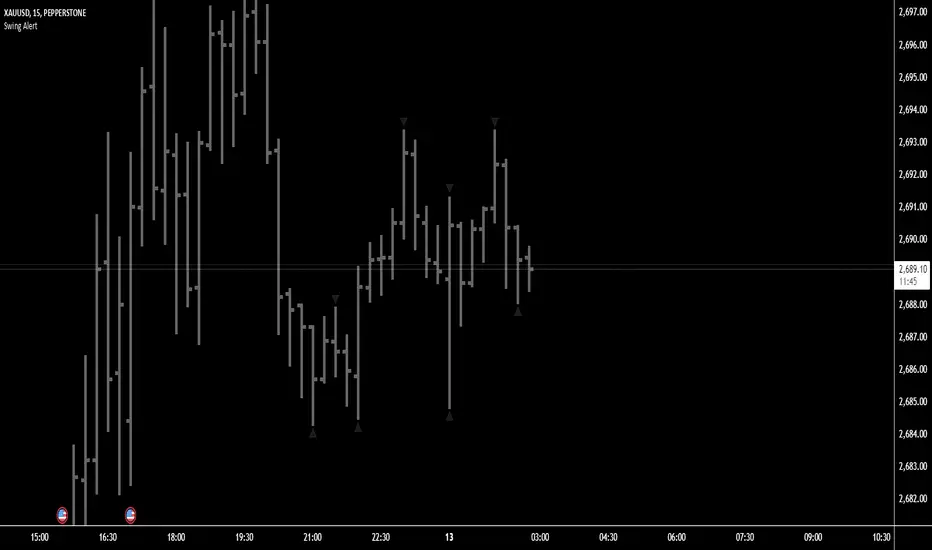
Swing Points AlertSwing Points Alert with Adjustable Delay
Description:
This script is designed to detect and alert traders about significant swing highs and lows on the chart. The script is equipped with customizable pivot detection settings and an innovative **Alert Delay** mechanism, allowing users to fine-tune their notifications to reduce noise and focus on key price movements.
Key Features:
1. **Swing High/Low Detection:**
- Identifies swing highs and lows based on user-defined pivot length.
- Visualizes these points with customizable labels for clarity.
2. **Customizable Alerts:**
- Enables real-time alerts for swing highs and lows.
- Users can adjust the delay for alerts to avoid false signals during volatile periods.
3. **Dynamic Label Management:**
- Automatically manages the number of displayed swing point labels.
- Removes crossed or outdated labels based on user preferences.
4. **Flexible Label Styling:**
- Provides multiple label styles (e.g., triangles, circles, arrows) and color customization for both swing highs and lows.
How the Alert Delay Works:
The **Alert Delay** helps filter signals by introducing a delay before triggering alerts. The delay is calculated as follows:
**Alert Delay (%) x Time Frame = Alert Delay in Time Frame Units**
For example:
- If the **Alert Delay** is set to 30% and the timeframe is **15 minutes**, the alert will be triggered after a delay of:
\
This ensures the alert is triggered only if the swing high/low condition remains valid for at least 4.5 minutes.
Important Notes:
1. **Timeframe Sensitivity:**
- This script is optimized for use across various timeframes, but users must adjust the **Alert Delay** percentage to match their trading style and timeframe.
- For example, higher timeframes may require lower delay percentages for timely alerts.
2. **Customization Options:**
- Easily customize pivot detection length, alert delay, label styles, and colors to suit your preferences.
3. **Support:**
- If you encounter any challenges or need help optimizing the script for your specific trading scenario, feel free to reach out for assistance.
Statistics • Chi Square • P-value • SignificanceThe Statistics • Chi Square • P-value • Significance publication aims to provide a tool for combining different conditions and checking whether the outcome is significant using the Chi-Square Test and P-value.
🔶 USAGE
The basic principle is to compare two or more groups and check the results of a query test, such as asking men and women whether they want to see a romantic or non-romantic movie.
–––––––––––––––––––––––––––––––––––––––––––––
| | ROMANTIC | NON-ROMANTIC | ⬅︎ MOVIE |
–––––––––––––––––––––––––––––––––––––––––––––
| MEN | 2 | 8 | 10 |
–––––––––––––––––––––––––––––––––––––––––––––
| WOMEN | 7 | 3 | 10 |
–––––––––––––––––––––––––––––––––––––––––––––
|⬆︎ SEX | 10 | 10 | 20 |
–––––––––––––––––––––––––––––––––––––––––––––
We calculate the Chi-Square Formula, which is:
Χ² = Σ ( (Observed Value − Expected Value)² / Expected Value )
In this publication, this is:
chiSquare = 0.
for i = 0 to rows -1
for j = 0 to colums -1
observedValue = aBin.get(i).aFloat.get(j)
expectedValue = math.max(1e-12, aBin.get(i).aFloat.get(colums) * aBin.get(rows).aFloat.get(j) / sumT) //Division by 0 protection
chiSquare += math.pow(observedValue - expectedValue, 2) / expectedValue
Together with the 'Degree of Freedom', which is (rows − 1) × (columns − 1) , the P-value can be calculated.
In this case it is P-value: 0.02462
A P-value lower than 0.05 is considered to be significant. Statistically, women tend to choose a romantic movie more, while men prefer a non-romantic one.
Users have the option to choose a P-value, calculated from a standard table or through a math.ucla.edu - Javascript-based function (see references below).
Note that the population (10 men + 10 women = 20) is small, something to consider.
Either way, this principle is applied in the script, where conditions can be chosen like rsi, close, high, ...
🔹 CONDITION
Conditions are added to the left column ('CONDITION')
For example, previous rsi values (rsi ) between 0-100, divided in separate groups
🔹 CLOSE
Then, the movement of the last close is evaluated
UP when close is higher then previous close (close )
DOWN when close is lower then previous close
EQUAL when close is equal then previous close
It is also possible to use only 2 columns by adding EQUAL to UP or DOWN
UP
DOWN/EQUAL
or
UP/EQUAL
DOWN
In other words, when previous rsi value was between 80 and 90, this resulted in:
19 times a current close higher than previous close
14 times a current close lower than previous close
0 times a current close equal than previous close
However, the P-value tells us it is not statistical significant.
NOTE: Always keep in mind that past behaviour gives no certainty about future behaviour.
A vertical line is drawn at the beginning of the chosen population (max 4990)
Here, the results seem significant.
🔹 GROUPS
It is important to ensure that the groups are formed correctly. All possibilities should be present, and conditions should only be part of 1 group.
In the example above, the two top situations are acceptable; close against close can only be higher, lower or equal.
The two examples at the bottom, however, are very poorly constructed.
Several conditions can be placed in more than 1 group, and some conditions are not integrated into a group. Even if the results are significant, they are useless because of the group formation.
A population count is added as an aid to spot errors in group formation.
In this example, there is a discrepancy between the population and total count due to the absence of a condition.
The results when rsi was between 5-25 are not included, resulting in unreliable results.
🔹 PRACTICAL EXAMPLES
In this example, we have specific groups where the condition only applies to that group.
For example, the condition rsi > 55 and rsi <= 65 isn't true in another group.
Also, every possible rsi value (0 - 100) is present in 1 of the groups.
rsi > 15 and rsi <= 25 28 times UP, 19 times DOWN and 2 times EQUAL. P-value: 0.01171
When looking in detail and examining the area 15-25 RSI, we see this:
The population is now not representative (only checking for RSI between 15-25; all other RSI values are not included), so we can ignore the P-value in this case. It is merely to check in detail. In this case, the RSI values 23 and 24 seem promising.
NOTE: We should check what the close price did without any condition.
If, for example, the close price had risen 100 times out of 100, this would make things very relative.
In this case (at least two conditions need to be present), we set 1 condition at 'always true' and another at 'always false' so we'll get only the close values without any condition:
Changing the population or the conditions will change the P-value.
In the following example, the outcome is evaluated when:
close value from 1 bar back is higher than the close value from 2 bars back
close value from 1 bar back is lower/equal than the close value from 2 bars back
Or:
close value from 1 bar back is higher than the close value from 2 bars back
close value from 1 bar back is equal than the close value from 2 bars back
close value from 1 bar back is lower than the close value from 2 bars back
In both examples, all possibilities of close against close are included in the calculations. close can only by higher, equal or lower than close
Both examples have the results without a condition included (5 = 5 and 5 < 5) so one can compare the direction of current close.
🔶 NOTES
• Always keep in mind that:
Past behaviour gives no certainty about future behaviour.
Everything depends on time, cycles, events, fundamentals, technicals, ...
• This test only works for categorical data (data in categories), such as Gender {Men, Women} or color {Red, Yellow, Green, Blue} etc., but not numerical data such as height or weight. One might argue that such tests shouldn't use rsi, close, ... values.
• Consider what you're measuring
For example rsi of the current bar will always lead to a close higher than the previous close, since this is inherent to the rsi calculations.
• Be careful; often, there are na -values at the beginning of the series, which are not included in the calculations!
• Always keep in mind considering what the close price did without any condition
• The numbers must be large enough. Each entry must be five or more. In other words, it is vital to make the 'population' large enough.
• The code can be developed further, for example, by splitting UP, DOWN in close UP 1-2%, close UP 2-3%, close UP 3-4%, ...
• rsi can be supplemented with stochRSI, MFI, sma, ema, ...
🔶 SETTINGS
🔹 Population
• Choose the population size; in other words, how many bars you want to go back to. If fewer bars are available than set, this will be automatically adjusted.
🔹 Inputs
At least two conditions need to be chosen.
• Users can add up to 11 conditions, where each condition can contain two different conditions.
🔹 RSI
• Length
🔹 Levels
• Set the used levels as desired.
🔹 Levels
• P-value: P-value retrieved using a standard table method or a function.
• Used function, derived from Chi-Square Distribution Function; JavaScript
LogGamma(Z) =>
S = 1
+ 76.18009173 / Z
- 86.50532033 / (Z+1)
+ 24.01409822 / (Z+2)
- 1.231739516 / (Z+3)
+ 0.00120858003 / (Z+4)
- 0.00000536382 / (Z+5)
(Z-.5) * math.log(Z+4.5) - (Z+4.5) + math.log(S * 2.50662827465)
Gcf(float X, A) => // Good for X > A +1
A0=0., B0=1., A1=1., B1=X, AOLD=0., N=0
while (math.abs((A1-AOLD)/A1) > .00001)
AOLD := A1
N += 1
A0 := A1+(N-A)*A0
B0 := B1+(N-A)*B0
A1 := X*A0+N*A1
B1 := X*B0+N*B1
A0 := A0/B1
B0 := B0/B1
A1 := A1/B1
B1 := 1
Prob = math.exp(A * math.log(X) - X - LogGamma(A)) * A1
1 - Prob
Gser(X, A) => // Good for X < A +1
T9 = 1. / A
G = T9
I = 1
while (T9 > G* 0.00001)
T9 := T9 * X / (A + I)
G := G + T9
I += 1
G *= math.exp(A * math.log(X) - X - LogGamma(A))
Gammacdf(x, a) =>
GI = 0.
if (x<=0)
GI := 0
else if (x
Chisqcdf = Gammacdf(Z/2, DF/2)
Chisqcdf := math.round(Chisqcdf * 100000) / 100000
pValue = 1 - Chisqcdf
🔶 REFERENCES
mathsisfun.com, Chi-Square Test
Chi-Square Distribution Function

Liquidity Heatmap [BigBeluga]The Liquidity Heatmap is an indicator designed to spot possible resting liquidity or potential stop loss using volume or Open interest.
The Open interest is the total number of outstanding derivative contracts for an asset—such as options or futures—that have not been settled. Open interest keeps track of every open position in a particular contract rather than tracking the total volume traded.
The Volume is the total quantity of shares or contracts traded for the current timeframe.
🔶 HOW IT WORKS
Based on the user choice between Volume or OI, the idea is the same for both.
On each candle, we add the data (volume or OI) below or above (long or short) that should be the hypothetical liquidation levels; More color of the liquidity level = more reaction when the price goes through it.
Gradient color is calculated between an average of 2 points that the user can select. For example: 500, and the script will take the average of the highest data between 500 and 250 (half of the user's choice), and the gradient will be based on that.
If we take volume as an example, a big volume spike will mean a lot of long or short activity in that candle. A liquidity level will be displayed below/above the set leverage (4.5 = 20x leverage as an example) so when the price revisits that zone, all the 20x leverage should be liquidated.
Huge volume = a lot of activity
Huge OI = a lot of positions opened
More volume / OI will result in a stronger color that will generate a stronger reaction.
🔶 ROUTE
Here's an example of a route for long liquidity:
Enable the filter = consider only green candles.
Set the leverage to 4.5 (20x).
Choose Data = Volume.
Process:
A green candle is formed.
A liquidity level is established.
The level is placed below to simulate the 20x leverage.
Color is applied, considering the average volume within the chosen area.
Route completed.
🔶 FEATURE
Possibility to change the color of both long and short liquidity
Manual opacity value
Manual opacity average
Leverage
Autopilot - set a good average automatically of the opacity value
Enable both long or short liquidity visualization
Filtering - grab only red/green candle of the corresponding side or grab every candle
Data - nzVolume - Volume - nzOI - OI
🔶 TIPS
Since the limit of the line is 500, it's best to plot 2 scripts: one with only long and another with only short.
🔶 CONCLUSION
The liquidity levels are an interesting way to think about possible levels, and those are not real levels.

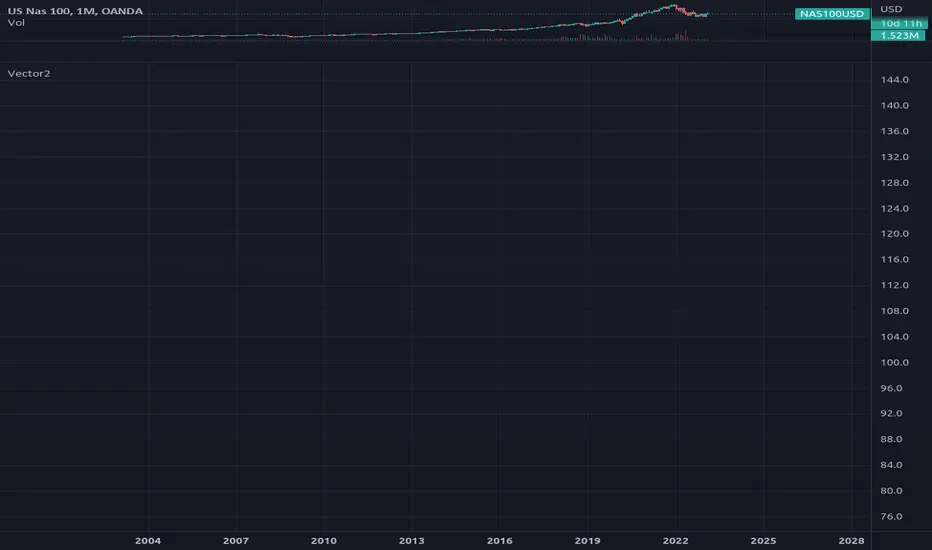
Vector2Library "Vector2"
Representation of two dimensional vectors or points.
This structure is used to represent positions in two dimensional space or vectors,
for example in spacial coordinates in 2D space.
~~~
references:
docs.unity3d.com
gist.github.com
github.com
gist.github.com
gist.github.com
gist.github.com
~~~
new(x, y)
Create a new Vector2 object.
Parameters:
x : float . The x value of the vector, default=0.
y : float . The y value of the vector, default=0.
Returns: Vector2. Vector2 object.
-> usage:
`unitx = Vector2.new(1.0) , plot(unitx.x)`
from(value)
Assigns value to a new vector `x,y` elements.
Parameters:
value : float, x and y value of the vector.
Returns: Vector2. Vector2 object.
-> usage:
`one = Vector2.from(1.0), plot(one.x)`
from(value, element_sep, open_par, close_par)
Assigns value to a new vector `x,y` elements.
Parameters:
value : string . The `x` and `y` value of the vector in a `x,y` or `(x,y)` format, spaces and parentesis will be removed automatically.
element_sep : string . Element separator character, default=`,`.
open_par : string . Open parentesis character, default=`(`.
close_par : string . Close parentesis character, default=`)`.
Returns: Vector2. Vector2 object.
-> usage:
`one = Vector2.from("1.0,2"), plot(one.x)`
copy(this)
Creates a deep copy of a vector.
Parameters:
this : Vector2 . Vector2 object.
Returns: Vector2. Vector2 object.
-> usage:
`a = Vector2.new(1.0) , b = a.copy() , plot(b.x)`
down()
Vector in the form `(0, -1)`.
Returns: Vector2. Vector2 object.
left()
Vector in the form `(-1, 0)`.
Returns: Vector2. Vector2 object.
right()
Vector in the form `(1, 0)`.
Returns: Vector2. Vector2 object.
up()
Vector in the form `(0, 1)`.
Returns: Vector2. Vector2 object.
one()
Vector in the form `(1, 1)`.
Returns: Vector2. Vector2 object.
zero()
Vector in the form `(0, 0)`.
Returns: Vector2. Vector2 object.
minus_one()
Vector in the form `(-1, -1)`.
Returns: Vector2. Vector2 object.
unit_x()
Vector in the form `(1, 0)`.
Returns: Vector2. Vector2 object.
unit_y()
Vector in the form `(0, 1)`.
Returns: Vector2. Vector2 object.
nan()
Vector in the form `(float(na), float(na))`.
Returns: Vector2. Vector2 object.
xy(this)
Return the values of `x` and `y` as a tuple.
Parameters:
this : Vector2 . Vector2 object.
Returns: .
-> usage:
`a = Vector2.new(1.0, 1.0) , = a.xy() , plot(ax)`
length_squared(this)
Length of vector `a` in the form. `a.x^2 + a.y^2`, for comparing vectors this is computationaly lighter.
Parameters:
this : Vector2 . Vector2 object.
Returns: float. Squared length of vector.
-> usage:
`a = Vector2.new(1.0, 1.0) , plot(a.length_squared())`
length(this)
Magnitude of vector `a` in the form. `sqrt(a.x^2 + a.y^2)`
Parameters:
this : Vector2 . Vector2 object.
Returns: float. Length of vector.
-> usage:
`a = Vector2.new(1.0, 1.0) , plot(a.length())`
normalize(a)
Vector normalized with a magnitude of 1, in the form. `a / length(a)`.
Parameters:
a : Vector2 . Vector2 object.
Returns: Vector2. Vector2 object.
-> usage:
`a = normalize(Vector2.new(3.0, 2.0)) , plot(a.y)`
isNA(this)
Checks if any of the components is `na`.
Parameters:
this : Vector2 . Vector2 object.
Returns: bool.
usage:
p = Vector2.new(1.0, na) , plot(isNA(p)?1:0)
add(a, b)
Adds vector `b` to `a`, in the form `(a.x + b.x, a.y + b.y)`.
Parameters:
a : Vector2 . Vector2 object.
b : Vector2 . Vector2 object.
Returns: Vector2. Vector2 object.
-> usage:
`a = one() , b = one() , c = add(a, b) , plot(c.x)`
add(a, b)
Adds vector `b` to `a`, in the form `(a.x + b, a.y + b)`.
Parameters:
a : Vector2 . Vector2 object.
b : float . Value.
Returns: Vector2. Vector2 object.
-> usage:
`a = one() , b = 1.0 , c = add(a, b) , plot(c.x)`
add(a, b)
Adds vector `b` to `a`, in the form `(a + b.x, a + b.y)`.
Parameters:
a : float . Value.
b : Vector2 . Vector2 object.
Returns: Vector2. Vector2 object.
-> usage:
`a = 1.0 , b = one() , c = add(a, b) , plot(c.x)`
subtract(a, b)
Subtract vector `b` from `a`, in the form `(a.x - b.x, a.y - b.y)`.
Parameters:
a : Vector2 . Vector2 object.
b : Vector2 . Vector2 object.
Returns: Vector2. Vector2 object.
-> usage:
`a = one() , b = one() , c = subtract(a, b) , plot(c.x)`
subtract(a, b)
Subtract vector `b` from `a`, in the form `(a.x - b, a.y - b)`.
Parameters:
a : Vector2 . vector2 object.
b : float . Value.
Returns: Vector2. Vector2 object.
-> usage:
`a = one() , b = 1.0 , c = subtract(a, b) , plot(c.x)`
subtract(a, b)
Subtract vector `b` from `a`, in the form `(a - b.x, a - b.y)`.
Parameters:
a : float . value.
b : Vector2 . Vector2 object.
Returns: Vector2. Vector2 object.
-> usage:
`a = 1.0 , b = one() , c = subtract(a, b) , plot(c.x)`
multiply(a, b)
Multiply vector `a` with `b`, in the form `(a.x * b.x, a.y * b.y)`.
Parameters:
a : Vector2 . Vector2 object.
b : Vector2 . Vector2 object.
Returns: Vector2. Vector2 object.
-> usage:
`a = one() , b = one() , c = multiply(a, b) , plot(c.x)`
multiply(a, b)
Multiply vector `a` with `b`, in the form `(a.x * b, a.y * b)`.
Parameters:
a : Vector2 . Vector2 object.
b : float . Value.
Returns: Vector2. Vector2 object.
-> usage:
`a = one() , b = 1.0 , c = multiply(a, b) , plot(c.x)`
multiply(a, b)
Multiply vector `a` with `b`, in the form `(a * b.x, a * b.y)`.
Parameters:
a : float . Value.
b : Vector2 . Vector2 object.
Returns: Vector2. Vector2 object.
-> usage:
`a = 1.0 , b = one() , c = multiply(a, b) , plot(c.x)`
divide(a, b)
Divide vector `a` with `b`, in the form `(a.x / b.x, a.y / b.y)`.
Parameters:
a : Vector2 . Vector2 object.
b : Vector2 . Vector2 object.
Returns: Vector2. Vector2 object.
-> usage:
`a = from(3.0) , b = from(2.0) , c = divide(a, b) , plot(c.x)`
divide(a, b)
Divide vector `a` with value `b`, in the form `(a.x / b, a.y / b)`.
Parameters:
a : Vector2 . Vector2 object.
b : float . Value.
Returns: Vector2. Vector2 object.
-> usage:
`a = from(3.0) , b = 2.0 , c = divide(a, b) , plot(c.x)`
divide(a, b)
Divide value `a` with vector `b`, in the form `(a / b.x, a / b.y)`.
Parameters:
a : float . Value.
b : Vector2 . Vector2 object.
Returns: Vector2. Vector2 object.
-> usage:
`a = 3.0 , b = from(2.0) , c = divide(a, b) , plot(c.x)`
negate(a)
Negative of vector `a`, in the form `(-a.x, -a.y)`.
Parameters:
a : Vector2 . Vector2 object.
Returns: Vector2. Vector2 object.
-> usage:
`a = from(3.0) , b = a.negate , plot(b.x)`
pow(a, b)
Raise vector `a` with exponent vector `b`, in the form `(a.x ^ b.x, a.y ^ b.y)`.
Parameters:
a : Vector2 . Vector2 object.
b : Vector2 . Vector2 object.
Returns: Vector2. Vector2 object.
-> usage:
`a = from(3.0) , b = from(2.0) , c = pow(a, b) , plot(c.x)`
pow(a, b)
Raise vector `a` with value `b`, in the form `(a.x ^ b, a.y ^ b)`.
Parameters:
a : Vector2 . Vector2 object.
b : float . Value.
Returns: Vector2. Vector2 object.
-> usage:
`a = from(3.0) , b = 2.0 , c = pow(a, b) , plot(c.x)`
pow(a, b)
Raise value `a` with vector `b`, in the form `(a ^ b.x, a ^ b.y)`.
Parameters:
a : float . Value.
b : Vector2 . Vector2 object.
Returns: Vector2. Vector2 object.
-> usage:
`a = 3.0 , b = from(2.0) , c = pow(a, b) , plot(c.x)`
sqrt(a)
Square root of the elements in a vector.
Parameters:
a : Vector2 . Vector2 object.
Returns: Vector2. Vector2 object.
-> usage:
`a = from(3.0) , b = sqrt(a) , plot(b.x)`
abs(a)
Absolute properties of the vector.
Parameters:
a : Vector2 . Vector2 object.
Returns: Vector2. Vector2 object.
-> usage:
`a = from(-3.0) , b = abs(a) , plot(b.x)`
min(a)
Lowest element of a vector.
Parameters:
a : Vector2 . Vector2 object.
Returns: float.
-> usage:
`a = new(3.0, 1.5) , b = min(a) , plot(b)`
max(a)
Highest element of a vector.
Parameters:
a : Vector2 . Vector2 object.
Returns: float.
-> usage:
`a = new(3.0, 1.5) , b = max(a) , plot(b)`
vmax(a, b)
Highest elements of two vectors.
Parameters:
a : Vector2 . Vector2 object.
b : Vector2 . Vector2 object.
Returns: Vector2. Vector2 object.
-> usage:
`a = new(3.0, 2.0) , b = new(2.0, 3.0) , c = vmax(a, b) , plot(c.x)`
vmax(a, b, c)
Highest elements of three vectors.
Parameters:
a : Vector2 . Vector2 object.
b : Vector2 . Vector2 object.
c : Vector2 . Vector2 object.
Returns: Vector2. Vector2 object.
-> usage:
`a = new(3.0, 2.0) , b = new(2.0, 3.0) , c = new(1.5, 4.5) , d = vmax(a, b, c) , plot(d.x)`
vmin(a, b)
Lowest elements of two vectors.
Parameters:
a : Vector2 . Vector2 object.
b : Vector2 . Vector2 object.
Returns: Vector2. Vector2 object.
-> usage:
`a = new(3.0, 2.0) , b = new(2.0, 3.0) , c = vmin(a, b) , plot(c.x)`
vmin(a, b, c)
Lowest elements of three vectors.
Parameters:
a : Vector2 . Vector2 object.
b : Vector2 . Vector2 object.
c : Vector2 . Vector2 object.
Returns: Vector2. Vector2 object.
-> usage:
`a = new(3.0, 2.0) , b = new(2.0, 3.0) , c = new(1.5, 4.5) , d = vmin(a, b, c) , plot(d.x)`
perp(a)
Perpendicular Vector of `a`, in the form `(a.y, -a.x)`.
Parameters:
a : Vector2 . Vector2 object.
Returns: Vector2. Vector2 object.
-> usage:
`a = new(3.0, 1.5) , b = perp(a) , plot(b.x)`
floor(a)
Compute the floor of vector `a`.
Parameters:
a : Vector2 . Vector2 object.
Returns: Vector2. Vector2 object.
-> usage:
`a = new(3.0, 1.5) , b = floor(a) , plot(b.x)`
ceil(a)
Ceils vector `a`.
Parameters:
a : Vector2 . Vector2 object.
Returns: Vector2. Vector2 object.
-> usage:
`a = new(3.0, 1.5) , b = ceil(a) , plot(b.x)`
ceil(a, digits)
Ceils vector `a`.
Parameters:
a : Vector2 . Vector2 object.
digits : int . Digits to use as ceiling.
Returns: Vector2. Vector2 object.
round(a)
Round of vector elements.
Parameters:
a : Vector2 . Vector2 object.
Returns: Vector2. Vector2 object.
-> usage:
`a = new(3.0, 1.5) , b = round(a) , plot(b.x)`
round(a, precision)
Round of vector elements.
Parameters:
a : Vector2 . Vector2 object.
precision : int . Number of digits to round vector "a" elements.
Returns: Vector2. Vector2 object.
-> usage:
`a = new(0.123456, 1.234567) , b = round(a, 2) , plot(b.x)`
fractional(a)
Compute the fractional part of the elements from vector `a`.
Parameters:
a : Vector2 . Vector2 object.
Returns: Vector2. Vector2 object.
-> usage:
`a = new(3.123456, 1.23456) , b = fractional(a) , plot(b.x)`
dot_product(a, b)
dot_product product of 2 vectors, in the form `a.x * b.x + a.y * b.y.
Parameters:
a : Vector2 . Vector2 object.
b : Vector2 . Vector2 object.
Returns: float.
-> usage:
`a = new(3.0, 1.5) , b = from(2.0) , c = dot_product(a, b) , plot(c)`
cross_product(a, b)
cross product of 2 vectors, in the form `a.x * b.y - a.y * b.x`.
Parameters:
a : Vector2 . Vector2 object.
b : Vector2 . Vector2 object.
Returns: float.
-> usage:
`a = new(3.0, 1.5) , b = from(2.0) , c = cross_product(a, b) , plot(c)`
equals(a, b)
Compares two vectors
Parameters:
a : Vector2 . Vector2 object.
b : Vector2 . Vector2 object.
Returns: bool. Representing the equality.
-> usage:
`a = new(3.0, 1.5) , b = from(2.0) , c = equals(a, b) ? 1 : 0 , plot(c)`
sin(a)
Compute the sine of argument vector `a`.
Parameters:
a : Vector2 . Vector2 object.
Returns: Vector2. Vector2 object.
-> usage:
`a = new(3.0, 1.5) , b = sin(a) , plot(b.x)`
cos(a)
Compute the cosine of argument vector `a`.
Parameters:
a : Vector2 . Vector2 object.
Returns: Vector2. Vector2 object.
-> usage:
`a = new(3.0, 1.5) , b = cos(a) , plot(b.x)`
tan(a)
Compute the tangent of argument vector `a`.
Parameters:
a : Vector2 . Vector2 object.
Returns: Vector2. Vector2 object.
-> usage:
`a = new(3.0, 1.5) , b = tan(a) , plot(b.x)`
atan2(x, y)
Approximation to atan2 calculation, arc tangent of `y/x` in the range (-pi,pi) radians.
Parameters:
x : float . The x value of the vector.
y : float . The y value of the vector.
Returns: float. Value with angle in radians. (negative if quadrante 3 or 4)
-> usage:
`a = new(3.0, 1.5) , b = atan2(a.x, a.y) , plot(b)`
atan2(a)
Approximation to atan2 calculation, arc tangent of `y/x` in the range (-pi,pi) radians.
Parameters:
a : Vector2 . Vector2 object.
Returns: float, value with angle in radians. (negative if quadrante 3 or 4)
-> usage:
`a = new(3.0, 1.5) , b = atan2(a) , plot(b)`
distance(a, b)
Distance between vector `a` and `b`.
Parameters:
a : Vector2 . Vector2 object.
b : Vector2 . Vector2 object.
Returns: float.
-> usage:
`a = new(3.0, 1.5) , b = from(2.0) , c = distance(a, b) , plot(c)`
rescale(a, length)
Rescale a vector to a new magnitude.
Parameters:
a : Vector2 . Vector2 object.
length : float . Magnitude.
Returns: Vector2. Vector2 object.
-> usage:
`a = new(3.0, 1.5) , b = 2.0 , c = rescale(a, b) , plot(c.x)`
rotate(a, radians)
Rotates vector by a angle.
Parameters:
a : Vector2 . Vector2 object.
radians : float . Angle value in radians.
Returns: Vector2. Vector2 object.
-> usage:
`a = new(3.0, 1.5) , b = 2.0 , c = rotate(a, b) , plot(c.x)`
rotate_degree(a, degree)
Rotates vector by a angle.
Parameters:
a : Vector2 . Vector2 object.
degree : float . Angle value in degrees.
Returns: Vector2. Vector2 object.
-> usage:
`a = new(3.0, 1.5) , b = 45.0 , c = rotate_degree(a, b) , plot(c.x)`
rotate_around(this, center, angle)
Rotates vector `target` around `origin` by angle value.
Parameters:
this
center : Vector2 . Vector2 object.
angle : float . Angle value in degrees.
Returns: Vector2. Vector2 object.
-> usage:
`a = new(3.0, 1.5) , b = from(2.0) , c = rotate_around(a, b, 45.0) , plot(c.x)`
perpendicular_distance(a, b, c)
Distance from point `a` to line between `b` and `c`.
Parameters:
a : Vector2 . Vector2 object.
b : Vector2 . Vector2 object.
c : Vector2 . Vector2 object.
Returns: float.
-> usage:
`a = new(1.5, 2.6) , b = from(1.0) , c = from(3.0) , d = perpendicular_distance(a, b, c) , plot(d.x)`
project(a, axis)
Project a vector onto another.
Parameters:
a : Vector2 . Vector2 object.
axis : Vector2 . Vector2 object.
Returns: Vector2. Vector2 object.
-> usage:
`a = new(3.0, 1.5) , b = from(2.0) , c = project(a, b) , plot(c.x)`
projectN(a, axis)
Project a vector onto a vector of unit length.
Parameters:
a : Vector2 . Vector2 object.
axis : Vector2 . Vector2 object.
Returns: Vector2. Vector2 object.
-> usage:
`a = new(3.0, 1.5) , b = from(2.0) , c = projectN(a, b) , plot(c.x)`
reflect(a, axis)
Reflect a vector on another.
Parameters:
a : Vector2 . Vector2 object.
axis
Returns: Vector2. Vector2 object.
-> usage:
`a = new(3.0, 1.5) , b = from(2.0) , c = reflect(a, b) , plot(c.x)`
reflectN(a, axis)
Reflect a vector to a arbitrary axis.
Parameters:
a : Vector2 . Vector2 object.
axis
Returns: Vector2. Vector2 object.
-> usage:
`a = new(3.0, 1.5) , b = from(2.0) , c = reflectN(a, b) , plot(c.x)`
angle(a)
Angle in radians of a vector.
Parameters:
a : Vector2 . Vector2 object.
Returns: float.
-> usage:
`a = new(3.0, 1.5) , b = angle(a) , plot(b)`
angle_unsigned(a, b)
unsigned degree angle between 0 and +180 by given two vectors.
Parameters:
a : Vector2 . Vector2 object.
b : Vector2 . Vector2 object.
Returns: float.
-> usage:
`a = new(3.0, 1.5) , b = from(2.0) , c = angle_unsigned(a, b) , plot(c)`
angle_signed(a, b)
Signed degree angle between -180 and +180 by given two vectors.
Parameters:
a : Vector2 . Vector2 object.
b : Vector2 . Vector2 object.
Returns: float.
-> usage:
`a = new(3.0, 1.5) , b = from(2.0) , c = angle_signed(a, b) , plot(c)`
angle_360(a, b)
Degree angle between 0 and 360 by given two vectors
Parameters:
a : Vector2 . Vector2 object.
b : Vector2 . Vector2 object.
Returns: float.
-> usage:
`a = new(3.0, 1.5) , b = from(2.0) , c = angle_360(a, b) , plot(c)`
clamp(a, min, max)
Restricts a vector between a min and max value.
Parameters:
a : Vector2 . Vector2 object.
min
max
Returns: Vector2. Vector2 object.
-> usage:
`a = new(3.0, 1.5) , b = from(2.0) , c = from(2.5) , d = clamp(a, b, c) , plot(d.x)`
clamp(a, min, max)
Restricts a vector between a min and max value.
Parameters:
a : Vector2 . Vector2 object.
min : float . Lower boundary value.
max : float . Higher boundary value.
Returns: Vector2. Vector2 object.
-> usage:
`a = new(3.0, 1.5) , b = clamp(a, 2.0, 2.5) , plot(b.x)`
lerp(a, b, rate)
Linearly interpolates between vectors a and b by rate.
Parameters:
a : Vector2 . Vector2 object.
b : Vector2 . Vector2 object.
rate : float . Value between (a:-infinity -> b:1.0), negative values will move away from b.
Returns: Vector2. Vector2 object.
-> usage:
`a = new(3.0, 1.5) , b = from(2.0) , c = lerp(a, b, 0.5) , plot(c.x)`
herp(a, b, rate)
Hermite curve interpolation between vectors a and b by rate.
Parameters:
a : Vector2 . Vector2 object.
b : Vector2 . Vector2 object.
rate : Vector2 . Vector2 object. Value between (a:0 > 1:b).
Returns: Vector2. Vector2 object.
-> usage:
`a = new(3.0, 1.5) , b = from(2.0) , c = from(2.5) , d = herp(a, b, c) , plot(d.x)`
transform(position, mat)
Transform a vector by the given matrix.
Parameters:
position : Vector2 . Source vector.
mat : M32 . Transformation matrix
Returns: Vector2. Transformed vector.
transform(position, mat)
Transform a vector by the given matrix.
Parameters:
position : Vector2 . Source vector.
mat : M44 . Transformation matrix
Returns: Vector2. Transformed vector.
transform(position, mat)
Transform a vector by the given matrix.
Parameters:
position : Vector2 . Source vector.
mat : matrix . Transformation matrix, requires a 3x2 or a 4x4 matrix.
Returns: Vector2. Transformed vector.
transform(this, rotation)
Transform a vector by the given quaternion rotation value.
Parameters:
this : Vector2 . Source vector.
rotation : Quaternion . Rotation to apply.
Returns: Vector2. Transformed vector.
area_triangle(a, b, c)
Find the area in a triangle of vectors.
Parameters:
a : Vector2 . Vector2 object.
b : Vector2 . Vector2 object.
c : Vector2 . Vector2 object.
Returns: float.
-> usage:
`a = new(1.0, 2.0) , b = from(2.0) , c = from(1.0) , d = area_triangle(a, b, c) , plot(d.x)`
random(max)
2D random value.
Parameters:
max : Vector2 . Vector2 object. Vector upper boundary.
Returns: Vector2. Vector2 object.
-> usage:
`a = from(2.0) , b = random(a) , plot(b.x)`
random(max)
2D random value.
Parameters:
max : float, Vector upper boundary.
Returns: Vector2. Vector2 object.
-> usage:
`a = random(2.0) , plot(a.x)`
random(min, max)
2D random value.
Parameters:
min : Vector2 . Vector2 object. Vector lower boundary.
max : Vector2 . Vector2 object. Vector upper boundary.
Returns: Vector2. Vector2 object.
-> usage:
`a = from(1.0) , b = from(2.0) , c = random(a, b) , plot(c.x)`
random(min, max)
2D random value.
Parameters:
min : Vector2 . Vector2 object. Vector lower boundary.
max : Vector2 . Vector2 object. Vector upper boundary.
Returns: Vector2. Vector2 object.
-> usage:
`a = random(1.0, 2.0) , plot(a.x)`
noise(a)
2D Noise based on Morgan McGuire @morgan3d.
Parameters:
a : Vector2 . Vector2 object.
Returns: Vector2. Vector2 object.
-> usage:
`a = from(2.0) , b = noise(a) , plot(b.x)`
to_string(a)
Converts vector `a` to a string format, in the form `"(x, y)"`.
Parameters:
a : Vector2 . Vector2 object.
Returns: string. In `"(x, y)"` format.
-> usage:
`a = from(2.0) , l = barstate.islast ? label.new(bar_index, 0.0, to_string(a)) : label(na)`
to_string(a, format)
Converts vector `a` to a string format, in the form `"(x, y)"`.
Parameters:
a : Vector2 . Vector2 object.
format : string . Format to apply transformation.
Returns: string. In `"(x, y)"` format.
-> usage:
`a = from(2.123456) , l = barstate.islast ? label.new(bar_index, 0.0, to_string(a, "#.##")) : label(na)`
to_array(a)
Converts vector to a array format.
Parameters:
a : Vector2 . Vector2 object.
Returns: array.
-> usage:
`a = from(2.0) , b = to_array(a) , plot(array.get(b, 0))`
to_barycentric(this, a, b, c)
Captures the barycentric coordinate of a cartesian position in the triangle plane.
Parameters:
this : Vector2 . Source cartesian coordinate position.
a : Vector2 . Triangle corner `a` vertice.
b : Vector2 . Triangle corner `b` vertice.
c : Vector2 . Triangle corner `c` vertice.
Returns: bool.
from_barycentric(this, a, b, c)
Captures the cartesian coordinate of a barycentric position in the triangle plane.
Parameters:
this : Vector2 . Source barycentric coordinate position.
a : Vector2 . Triangle corner `a` vertice.
b : Vector2 . Triangle corner `b` vertice.
c : Vector2 . Triangle corner `c` vertice.
Returns: bool.
to_complex(this)
Translate a Vector2 structure to complex.
Parameters:
this : Vector2 . Source vector.
Returns: Complex.
to_polar(this)
Translate a Vector2 cartesian coordinate into polar coordinates.
Parameters:
this : Vector2 . Source vector.
Returns: Pole. The returned angle is in radians.
Overlay Mini Plot(s) of Correlated Asset(s)Overlay a small plot of a correlated asset of your choosing. Shrink/expand, Set vertical and horizontal position, plot multiple mini-plots via duplicate indicators with varied settings.
Plots the last X bars of any asset; including the live candle currently painting
Useful for low time frame trading when you want to see correlated asset price movement right alongside the price movement you're watching.
Useful for quick and simple comparisons; when you don't want the clutter of split screen or multi-pane view.
Useful for backtesting.
Price scale agnostic; just plots the shape of the recent price action, with several optional labels: Asset+timeframe | Live Price | Highest price over X bars | Lowest price over X bars.
Works fine with all the assets i've tested it on.
~~User inputs~~
-number of bars to paint.
-horizontal offset: plot to right X bars or to left X bars
-vertical offset: shift up or down, shrink or expand; by using 2 'spacer' inputs
-color/transparancy of candles and price labels.
-width (pixels) of candle bodies.
-choose to display price labels or not
-choose to display asset label or not
~~Tips~~
--Add several of these indicators; changing the vertical 'Shift/Shrink' settings on each to visually separate them.
--In the above chart or EurUsd, there are three indicators =>> three mini-plots overlaid: DXY, EurGbp and GbpUsd. Using the following settings for Space Above:Space Below: DXY- 0.1:4.5 | EurGbp- 1.8:1.8 | GbpUsd- 4.5:0.1
--the more you add, the more you'll have to vertically shrink the plots
© twingall

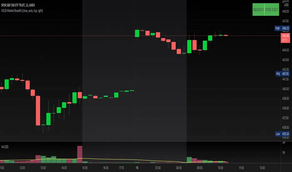
VOLD-MarketBreadth-RatioThis script provides NASDAQ and NYSE Up Volume (volume in rising stocks) and Down Volume (volume in falling stocks) ratio. Up Volume is higher than Down Volume, then you would see green label with ratio e.g 3.5:1. This means Up Volume is 3.5 times higher than Down Volume - Positive Market Breadth. If Down Volume is higher than Up Volume, then you would see red label with ratio e.g -4.5:1. This means Down Volume is 4.5 times higher than Up Volume.
For example, ratio is 1:1, then it is considered Market Breadth is Neutral.
PS: Currently TradingView provides only NASDAQ Composite Market volume data. I have requested them to provide Primary NASDAQ volume data. If they respond with new ticket for primary NQ data, I will update the script and publish the updated version. So if you have got similar table on ToS, you would see minor difference in NQ ratio.
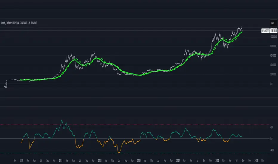
FUMO 200 MagnetWhat it does
FUMO Magnet measures how far price has stretched away from its long-term “magnet” — a blended EMA/SMA moving average (200 by default).
It plots a logarithmic deviation (optionally normalized) as an oscillator around zero.
Above 0** → price is above the magnet (stretched up)
Below 0** → price is below the magnet (stretched down)
Guide levels** highlight potential overbought/oversold zones
---
Why log deviation?
Log returns make extremes comparable across cycles and compress exponential trends — especially useful for BTC and other crypto assets.
Normalization modes further adjust the scale, keeping the oscillator readable on any chart.
---
Inputs
**Base**
* Source (default: Close)
* Base Length (default: 200 EMA/SMA)
* EMA vs SMA weight (%) — 0% = pure SMA, 100% = pure EMA, 50% = blended
* EMA smoothing of deviation — acts as a noise filter
**Normalization**
* None (Log Deviation) — raw log stretch in % terms
* Z-score — deviation in standard deviations (σ)
* Robust Z (MAD) — deviation vs median absolute deviation, resistant to outliers
* Tanh squash — smooth nonlinear squash of extremes for compact scale
* Normalization window (for Z / MAD)
* Tanh scale (lower = stronger squash)
* Clamp after normalization — hard cap at ±X
**Levels**
* Guide levels (Upper / Lower) — visual thresholds (default ±12)
* Zero line toggle
---
### How to read it
* **Trend bias**: sustained time above 0 = uptrend, below 0 = downtrend
* **Stretch / mean reversion**: the farther from 0, the higher the reversion risk
* **Cross-checks**: combine with structure (HH/HL, LH/LL), volume, or momentum (RSI, MACD)
---
### Recommended settings by timeframe
**Long-term (1D / 1W)**
* Normalization: None (Log Deviation)
* Base Length: 200
* EMA vs SMA weight: 50% (adjust 35–65% for faster/slower magnet)
* Deviation smoothing: 20 (10–30 range)
* Guide levels: ±12 to ±20
* Use case: cycle extremes, portfolio rebalancing, trim/add logic
**Swing (4H – 1D)**
* Normalization: Z-score
* Window: 200 (100–250)
* Smoothing: 14–20
* Guide levels: ±2σ to ±3σ
* Use case: stretched conditions across regimes; ±3σ is rare, often mean-reverts
**Intraday / Active swing (1H – 4H)**
* Normalization: Robust Z (MAD)
* Window: 200 (150 for faster response)
* Smoothing: 10–16
* Guide levels: ±3 to ±4 (robust units)
* Use case: handles spikes better than σ, fewer false overbought/oversold signals
**Scalping / Universal readability (15m – 1H)**
* Normalization: Tanh squash
* Tanh scale: 6–10 (start with 8)
* Smoothing: 8–12
* Guide levels: ±8 to ±12
* Use case: compact panel across assets and timeframes; not % or σ, but visually consistent
---
### Optional
* Clamp: enable ±20 (or ±25) for strict bounded range (useful for public charts)
---
### Quick setups
**BTC Daily (“cycle view”)**
* Normalization: None
* Blend: 50%
* Smooth: 20
* Levels: ±12–15
**BTC 4H (“swing”)**
* Normalization: Z-score
* Window: 200
* Smooth: 16
* Levels: ±2.5σ to ±3σ
**Alts 1H (“volatile”)**
* Normalization: Robust Z (MAD)
* Window: 200
* Smooth: 12
* Levels: ±3.5 to ±4.5
**Mixed assets 15m (“compact panel”)**
* Normalization: Tanh squash
* Scale: 8
* Smooth: 10
* Levels: ±8–12
* Clamp: ±20
Session Range ProjectionsSession Range Projections
Purpose & Concept:
Session Range Projections is a comprehensive trading tool that identifies and analyzes price ranges during user-defined time periods. The indicator visualizes high-probability reversal zones and profit targets by projecting Fibonacci levels from custom session ranges, making it ideal for traders who focus on time-based market structure analysis.
Key Features & Calculations:
1. Custom Time Range Analysis
- Define any time period for range calculation - from traditional sessions (Asian, London, NY) to custom periods like opening ranges, hourly ranges, or 4-hour blocks
- Automatically captures the highest and lowest prices within your specified timeframe
- Supports multiple timezone selections for global market analysis
- Flexible enough for intraday scalping ranges or longer-term swing trading setups
2. Premium & Discount Zones
- Automatically divides the range into premium (above 50%) and discount (below 50%) zones
- Visual differentiation helps identify institutional buying and selling areas
- Color-coded boxes clearly mark these critical price zones
3. Optimal Trade Entry (OTE) Zones
- Highlights the 79-89% retracement zone in premium territory
- Highlights the 11-21% retracement zone in discount territory
- These zones represent high-probability reversal areas based on institutional order flow concepts
4. Fibonacci Projections
- Projects 11 customizable Fibonacci extension levels from the range extremes
- Levels extend both above and below the range for symmetrical analysis
- Each level can be individually toggled and color-customized
- Default levels include common retracement ratios: -0.5, -1.0, -2.0, -2.33, -2.5, -3.0, -4.0, -4.5, -6.0, -7.0, -8.0
How to Use:
Set Your Time Range: Input your desired session start and end times (24-hour format)
Select Timezone: Choose the appropriate timezone for your trading session
Customize Display: Toggle various visual elements based on your preferences
Monitor Price Action: Watch for reactions at projected levels and OTE zones
Set Alerts: Configure sweep alerts for when price breaks above/below range extremes
Input Parameters Explained:
Time Range Settings
Range Start/End Hour & Minute: Define your analysis period
Time Zone: Ensure accurate session timing across different markets
Visual Settings
Range Box: Toggle the premium/discount zone visualization
Horizontal Lines: Customize high/low line appearance
Internal Range Levels: Show/hide equilibrium and OTE zones
Labels: Configure text display for key levels
Fibonacci Projections: Enable/disable extension levels
Display Settings
Historical Ranges: Show up to 10 previous session ranges
Alert Type: Choose between high sweep, low sweep, or both
Trading Applications:
Session-Based Trading: Analyze specific market sessions (Asian, London, New York, opening ranges, hourly ranges)
Reversal Trading: Identify high-probability reversal zones at OTE levels
Breakout/Reversal Trading: Monitor range breaks/reversals with built-in sweep alerts
Risk Management: Use Fibonacci projections as profit targets or rejection areas
Multi-Timeframe Analysis: Apply to any timeframe for various trading styles
Important Notes:
This indicator is for educational purposes only and should not be considered financial advice
Past performance does not guarantee future results
Always use proper risk management when trading
The indicator automatically manages historical data to maintain chart performance

Key Prices & LevelsThis indicator is designed to visualize key price levels & areas for NY trading sessions based on the price action from previous day, pre-market activity and key areas from NY session itself. The purpose is to unify all key levels into a single indicator, while allowing a user to control which levels they want to visualize and how.
The indicator identifies the following:
Asia Range High/Lows, along with ability to visualize with a box
London Range High/Lows, along with ability to visualize with a box
Previous Day PM Session High/Lows
Current Day Lunch Session High/Lows, starts appearing after 12pm EST once the lunch session starts
New York Open (8:30am EST) price
9:53 Open (root candle) price
New York Midnight (12:00am EST) price
Previous Day High/Lows
First 1m FVG after NY Session Start (after 9:30am), with the ability to configure minimum FVG size.
Opening Range Gap, showing regular market hours close price (previous day 16:15pm EST close), new session open price (9:30am EST open) and optionally the mid-point between the two
Asia Range 50% along with 2, 2.5, 4 and 4.5 deviations of the Asia range in both directions
Configurability:
Each price level can be turned off
Styles in terms of line type, color
Ability to turn on/off labels for price levels and highlighting of prices on price scale
Ability to control label text for price levels
How is it different:
Identifies novel concepts such as 9:53 open, root candle that can be used as a bounce/resistance area during AM/PM sessions as well as confirmation of direction once closed over/under to indicate price's willingness to continue moving in the same direction.
It also shows 1st 1m FVG after New York Session open, that can be used to determine direction of the price action depending on PA's reaction to that area. While both 9:53 and 1m FVG are 1m based markers, these levels are visualized by the indicator on all timeframes from 15s to 1h.
Additionally the indicator is able to both highlight key prices in the price scale pane as well as combine labels to minimize clutter when multiple levels have the same price.
Lastly for in-session ranges such as Lunch High/Low the indicator updates the range in real-time as opposed to waiting for the lunch session to be over.
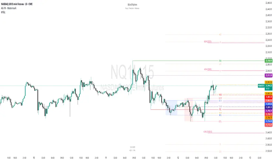
Open Liquidity Heatmap [BigBeluga]Open Liquidity Heatmap is an indicator designed to display accumulated resting liquidity on the chart.
Unlike any other liquidity heatmap, this aims to accumulate liquidity at specific levels that build up over time, showing larger areas of liquidity.
🔶 FEATURES
The indicator includes the following settings:
Lookback : Used to determine the range calculation of the heatmap.
Leverage : Leverage of the liquidation (Counted as % in price, Example: 4.5 will return a distance from price of 4.5%, indicating any possible resting liquidity in this range).
Levels : Amount of levels to display (Each level is counted as liquidity resting on the chart; fewer levels will return a bigger area of liquidity sitting on the chart).
Mode : Apply a color gradient from the minimum liquidation to the maximum liquidity level. Set the maximum color gradient value (Counted as volume).
Offset : Automatically determine the offset range of the Volume Profiles. Manual offset of the Volume Profiles.
🔶 CALCULATION
for i = 0 to step - 1
float plotter = na
switch i
0 =>
plotter := hs
=>
plotter := hs - diff * ( i )
cls.hm.gnL(plotter)
cls.vp.put(plotter, 0)
We calculate levels like a normal volume profile with steps, from the highest point within the lookback to the lowest one. Each level will contain the corresponding amount of volume that the candle has closed in that range.
As we can see in the image above, we add liquidity each time the distance in % from price is between two levels.
Unlike many liquidity indicators that provide a single candle liquidity heatmap, this aims to add up liquidity (volume) in already present levels.
This can be extremely useful to see which levels are likely to be more liquid and tend to get a bigger reaction to the price.
Imagine it like a range of levels that each time price revisits that area, a new position area is added; we add volume in that area each time price visits that zone. Liquidity builds up in those zones, causing a bigger reaction to the price once the price visits it.
This indicator is not the same as a single candle heatmap like many others. What is a single candle heatmap?
A single candle heatmap is when a level is created on every new candle, coloring the level based on the total volume of it.
This indicator, on the contrary, aims to provide a more specific use by adding up liquidity each time price visits it.
🔶 BASIC DEMOSTRATION
This is a basic demonstration of how we can spot high liquidity points overall using confluence:
We see the POC of the liquidation in a low volume area of the normal volume profile adding up as confluence.
Resistance from the POC Volume Profile suggesting price will go lower.
Major long open liquidity down.
As we can see, price takes out all the long liquidity and right after pumping, indicating that all the major liquidity got taken out.
Some key note to take is that a POC in the liquidation heatmap in a low volume area of the normal Volume Profile add confluence of a possible big reaction in that zone.
In the forex market, we suggest to use a low distance from price (Leverage) while in a crypto market you can use the one that fit the best the current timeframe.
🔶 CONCLUSION
This indicator aims to show open resting liquidity that had built up over time, showing the most amount of liquidation in specific areas in an aggregated way unlike many liquidation heatmap indicators that show single-level liquidation.
🔶 RELATED SCRIPT

ATR GOD Strategy by TradeSmart (PineConnector-compatible)This is a highly-customizable trading strategy made by TradeSmart, focusing mainly on ATR-based indicators and filters. The strategy is mainly intended for trading forex , and has been optimized using the Deep Backtest feature on the 2018.01.01 - 2023.06.01 interval on the EUR/USD (FXCM) 15M chart, with a Slippage value of 3, and a Commission set to 0.00004 USD per contract. The strategy is also made compatible with PineConnector , to provide an easy option to automate the strategy using a connection to MetaTrader. See tooltips for details on how to set up the bot, and check out our website for a detailed guide with images on how to automate the strategy.
The strategy was implemented using the following logic:
Entry strategy:
A total of 4 Supertrend values can be used to determine the entry logic. There is option to set up all 4 Supertrend parameters individually, as well as their potential to be used as an entry signal/or a trend filter. Long/Short entry signals will be determined based on the selected potential Supertrend entry signals, and filtered based on them being in an uptrend/downtrend (also available for setup). Please use the provided tooltips for each setup to see every detail.
Exit strategy:
4 different types of Stop Losses are available: ATR-based/Candle Low/High Based/Percentage Based/Pip Based. Additionally, Force exiting can also be applied, where there is option to set up 4 custom sessions, and exits will happen after the session has closed.
Parameters of every indicator used in the strategy can be tuned in the strategy settings as follows:
Plot settings:
Plot Signals: true by default, Show all Long and Short signals on the signal candle
Plot SL/TP lines: false by default, Checking this option will result in the TP and SL lines to be plotted on the chart.
Supertrend 1-4:
All the parameters of the Supertrends can be set up here, as well as their individual role in the entry logic.
Exit Strategy:
ATR Based Stop Loss: true by default
ATR Length (of the SL): 100 by default
ATR Smoothing (of the SL): RMA/SMMA by default
Candle Low/High Based Stop Loss: false by default, recent lowest or highest point (depending on long/short position) will be used to calculate stop loss value. Set 'Base Risk Multiplier' to 1 if you would like to use the calculated value as is. Setting it to a different value will count as an additional multiplier.
Candle Lookback (of the SL): 50 by default
Percentage Based Stop Loss: false by default, Set the stop loss to current price - % of current price (long) or price + % of current price (short).
Percentage (of the SL): 0.3 by default
Pip Based Stop Loss: Set the stop loss to current price - x pips (long) or price + x pips (short). Set 'Base Risk Multiplier' to 1 if you would like to use the calculated value as is. Setting it to a different value will count as an additional multiplier.
Pip (of the SL): 10 by default
Base Risk Multiplier: 4.5 by default, the stop loss will be placed at this risk level (meaning in case of ATR SL that the ATR value will be multiplied by this factor and the SL will be placed that value away from the entry level)
Risk to Reward Ratio: 1.5 by default, the take profit level will be placed such as this Risk/Reward ratio is met
Force Exiting:
4 total Force exit on custom session close options: none applied by default. If enabled, trades will close automatically after the set session is closed (on next candle's open).
Base Setups:
Allow Long Entries: true by default
Allow Short Entries: true by default
Order Size: 10 by default
Order Type: Capital Percentage by default, allows adjustment on how the position size is calculated: Cash: only the set cash amount will be used for each trade Contract(s): the adjusted number of contracts will be used for each trade Capital Percentage: a % of the current available capital will be used for each trade
ATR Limiter:
Use ATR Limiter: true by default, Only enter into any position (long/short) if ATR value is higher than the Low Boundary and lower than the High Boundary.
ATR Limiter Length: 50 by default
ATR Limiter Smoothing: RMA/SMMA by default
High Boundary: 1000 by default
Low Boundary: 0.0003 by default
MA based calculation: ATR value under MA by default, If not Unspecified, an MA is calculated with the ATR value as source. Only enter into position (long/short) if ATR value is higher/lower than the MA.
MA Type: RMA/SMMA by default
MA Length: 400 by default
Waddah Attar Filter:
Explosion/Deadzone relation: Not specified by default, Explosion over Deadzone: trades will only happen if the explosion line is over the deadzone line; Explosion under Deadzone: trades will only happen if the explosion line is under the deadzone line; Not specified: the opening of trades will not be based on the relation between the explosion and deadzone lines.
Limit trades based on trends: Not specified by default, Strong Trends: only enter long if the WA bar is colored green (there is an uptrend and the current bar is higher then the previous); only enter short if the WA bar is colored red (there is a downtrend and the current bar is higher then the previous); Soft Trends: only enter long if the WA bar is colored lime (there is an uptrend and the current bar is lower then the previous); only enter short if the WA bar is colored orange (there is a downtrend and the current bar is lower then the previous); All Trends: only enter long if the WA bar is colored green or lime (there is an uptrend); only enter short if the WA bar is colored red or orange (there is a downtrend); Not specified: the color of the WA bar (trend) is not relevant when considering entries.
WA bar value: Not specified by default, Over Explosion and Deadzone: only enter trades when the WA bar value is over the Explosion and Deadzone lines; Not specified: the relation between the explosion/deadzone lines to the value of the WA bar will not be used to filter opening trades.
Sensitivity: 150 by default
Fast MA Type: SMA by default
Fast MA Length: 10 by default
Slow MA Type: SMA
Slow MA Length: 20 by default
Channel MA Type: EMA by default
BB Channel Length: 20 by default
BB Stdev Multiplier: 2 by default
Trend Filter:
Use long trend filter 1: false by default, Only enter long if price is above Long MA.
Show long trend filter 1: false by default, Plot the selected MA on the chart.
TF1 - MA Type: EMA by default
TF1 - MA Length: 120 by default
TF1 - MA Source: close by default
Use short trend filter 1: false by default, Only enter long if price is above Long MA.
Show short trend filter 1: false by default, Plot the selected MA on the chart.
TF2 - MA Type: EMA by default
TF2 - MA Length: 120 by default
TF2 - MA Source: close by default
Volume Filter:
Only enter trades where volume is higher then the volume-based MA: true by default, a set type of MA will be calculated with the volume as source, and set length
MA Type: RMA/SMMA by default
MA Length: 200 by default
Date Range Limiter:
Limit Between Dates: false by default
Start Date: Jan 01 2023 00:00:00 by default
End Date: Jun 24 2023 00:00:00 by default
Session Limiter:
Show session plots: false by default, show market sessions on chart: Sidney (red), Tokyo (orange), London (yellow), New York (green)
Use session limiter: false by default, if enabled, trades will only happen in the ticked sessions below.
Sidney session: false by default, session between: 15:00 - 00:00 (EST)
Tokyo session: false by default, session between: 19:00 - 04:00 (EST)
London session: false by default, session between: 03:00 - 11:00 (EST)
New York session: false by default, session between: 08:00 - 17:00 (EST)
Trading Time:
Limit Trading Time: true by default, tick this together with the options below to enable limiting based on day and time
Valid Trading Days Global: 123567 by default, if the Limit Trading Time is on, trades will only happen on days that are present in this field. If any of the not global Valid Trading Days is used, this field will be neglected. Values represent days: Sunday (1), Monday (2), ..., Friday (6), Saturday(7) To trade on all days use: 123457
(1) Valid Trading Days: false, 123456 by default, values represent days: Sunday (1), Monday (2), ..., Friday (6), Saturday(7) The script will trade on days that are present in this field. Please make sure that this field and also (1) Valid Trading Hours Between is checked
(1) Valid Trading Hours Between: false, 1800-2000 by default, hours between which the trades can happen. The time is always in the exchange's timezone
All other options are also disabled by default
PineConnector Automation:
Use PineConnector Automation: false by default, In order for the connection to MetaTrader to work, you will need do perform prerequisite steps, you can follow our full guide at our website, or refer to the official PineConnector Documentation. To set up PineConnector Automation on the TradingView side, you will need to do the following:
1. Fill out the License ID field with your PineConnector License ID;
2. Fill out the Risk (trading volume) with the desired volume to be traded in each trade (the meaning of this value depends on the EA settings in Metatrader. Follow the detailed guide for additional information);
3. After filling out the fields, you need to enable the 'Use PineConnector Automation' option (check the box in the strategy settings);
4. Check if the chart has updated and you can see the appropriate order comments on your chart;
5. Create an alert with the strategy selected as Condition, and the Message as {{strategy.order.comment}} (should be there by default);
6. Enable the Webhook URL in the Notifications section, set it as the official PineConnector webhook address and enjoy your connection with MetaTrader.
License ID: 60123456789 by default
Risk (trading volume): 1 by default
NOTE! Fine-tuning/re-optimization is highly recommended when using other asset/timeframe combinations.
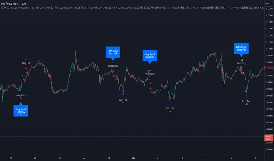
Centered Moving AverageThe Centered moving averages tries to resolve the problem that simple moving average are still not able to handle significant trends when forecasting.
When computing a running moving average in a centered way, placing the average in the middle time period makes sense.
If we average an even number of terms, we need to smooth the smoothed values.
Try to describe it with an example:
The following table shows the results using a centered moving average of 4.
nterim Steps
Period Value SMA Centered
1 9
1.5
2 8
2.5 9.5
3 9 9.5
3.5 9.5
4 12 10.0
4.5 10.5
5 9 10.750
5.5 11.0
6 12
6.5
7 11
This is the final table:
Period Value Centered MA
1 9
2 8
3 9 9.5
4 12 10.0
5 9 10.75
6 12
7 11
With this script we are able to process and display the centered moving average as described above.
In addition to this, however, the script is also able to estimate the potential projection of future data based on the available data by replicating where necessary the data of the last bar until the number of data necessary for the calculation of the required centered moving average is reached.
If for example I have 20 daily closings and I look for the moving average centered at 10, I receive the first data on the fifth day and the last data on the fourteenth day, so I have 5 days left uncovered, to remedy this I have to give the last value to the uncovered data the closing price of the last day.
The deviations work like the bollinger bands but must refer to the centered moving average.

[blackcat] L3 Candle Skew 3821 TraderLevel 3
Background
By modeling skew to produce long and short entry points.
Function
The concept of skew comes from physics and statistics, and is used in market technical analysis to reflect the expectation of future stock price distribution. Because the return distribution of stocks in the trend market has skew (Skew), it is reasonable to judge the trend continuity according to the historical and current skew. It is precisely because the stock price rises that there is a skew. The greater the strength of the rise, the greater the angle of inclination and the greater the skew. The degree of this upward or downward slope in the statistical distribution of stock prices is defined as skew. Through the size of skew, we can know the direction, inertia and extent of the stock's rise or fall, and find stocks with a high probability of quick profit. The technical indicator introduced today is a simplified but effective stock price skew model used to generate buying and selling points.
The principle of this technical indicator is based on the success rate test results of different moving averages corresponding to different skews as follows:
10 trading cycles profit 5% success rate (%)
5 period moving average 10 period moving average 20 period moving average 30 period moving average 60 period moving average
skew>=0 51.36 52.26 52.65 52.55 52.08
skew>=0.5 55.44 58.06 60.56 62.37 65.66
skew>=1 59.72 63.06 67.07 69.78 70.62
skew>=1.5 63.01 67.08 71.61 72.9 70.61
skew>=2 65.53 70.22 74.18 73.76 70.12
skew>=2.5 67.89 72.93 75.32 73.66 68.92
skew>=3 70.07 75.32 75.69 72.54 67.45
skew>=3.5 71.85 77.05 75.32 73.63 63.82
skew>=4 73.6 78.06 74.19 68.96 59.91
skew>=4.5 76.04 78.56 72.85 69.55 49.24
skew>=5 77.44 78.88 71.58 67.28 51.69
skew>=5.5 78.97 78.39 70.33 64.31 49.7
skew>=6 79.68 78.07 68.82 61.65 53.57
Table 1
As can be seen from the above table, with the increase of the 5-period and 10-period moving average skew values, the success rate is increasing, but after the 20- and 30-period moving average skew values increase to an upper bound, it shows a downward trend. When the skew of the 20-period and 30-period moving averages is greater than 0.5, the 10-period profit of 5% is above 60%, and when it is greater than 1.5, the success rate can reach above 70%. The larger the 5-period moving average skew, the higher the success rate, but often because the short-term skew is too large, the stock price has risen rapidly to a high level, and chasing up is risky, which is not suitable for the investment habits of most people, so prudent investors may like to do swings. Investors may wish to pay more attention to the skew of the 20-period and 30-period moving averages. Based on the above analysis, as a short-term trading enthusiast, I need to choose the 5-period and 10-period moving average skew, and consider the medium-term trend as a compromise, and I also need to consider the 20-period moving average skew. Finally, according to the principle of personal preference, I chose 3 groups of periods based on Fibonacci magic numbers: 3 periods, 8 periods, 21 periods, and skews that take into account both short-term and mid-line trends. So, I named this indicator number 3821 as a distinction.
002084 1D from TradingView
BTCUSDT 1H from TradingView
Tesla 1D from TradingView
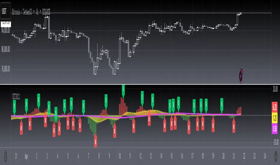
Roc Mean Reversion (ValueRay)This Indicator shows the Absolute Rate of Change in correlation to its Moving Average.
Values over 3 (gray dotted line) can savely be considered as a breakout; values over 4.5 got a high mean-reverting chance (red dotted line).
This Indicator can be used in all timeframes, however, i recommend to use it <30m, when you want search for meaningful Mean-Reverting Signals.
Please like, share and subscribe. With your love, im encouraged to write and publish more Indicators.
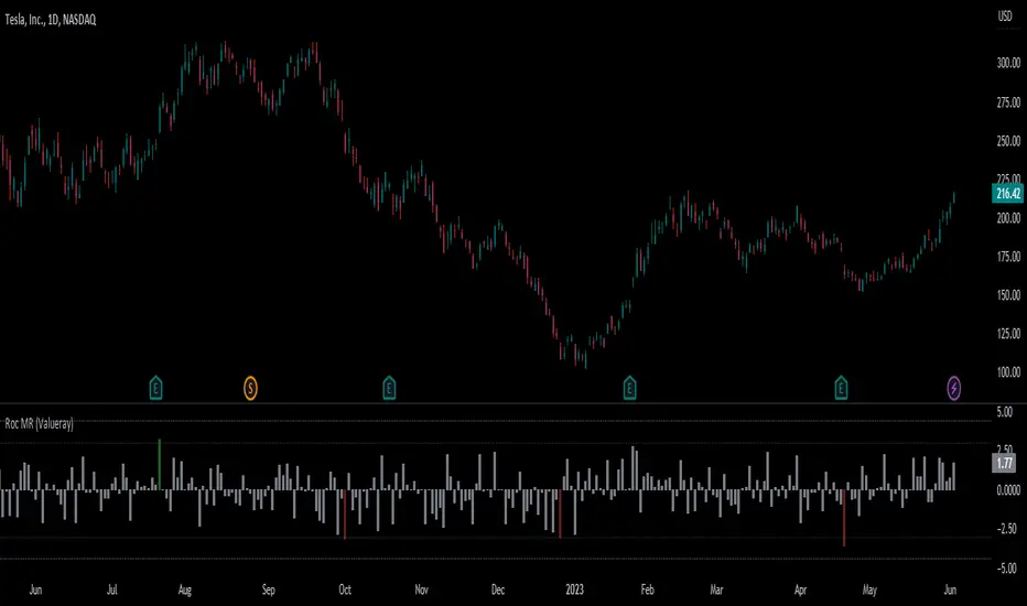
Cosmic Bands4 Bollinger Band channels with StdDev mult values of 1, 2, 4, and 4.5 (the last value can be changed in the indicator's settings).
Often shows better correlation with the log setting on.
