Linh Index Trend & Exhaustion SuitePurpose: One overlay to judge trend, reversal risk, overextension, and volatility squeezes on indexes (built for VNINDEX/VN30, works on any symbol & timeframe).
What it shows
Trend state: Bull / Bear / Transition via 20/50/200 EMAs + slope check.
Overextension heatmap: Background paints when price is stretched vs the 20-EMA by ATR or % (you set the thresholds).
Squeeze detection:
Squeeze ON (yellow dot): Bollinger Bands (20,2) inside Keltner Channels (20,1.5).
Squeeze OFF + Release: White dot; script confirms direction only when close > BB upper (up) or close < BB lower (down).
52-week context: Distance to 52-week high/low (%).
Higher-TF alignment: Optional weekly trend reading shown on the label while you’re on the daily.
Anchored VWAP(s): Two optional AVWAPs from dates you choose (e.g., YTD open, last big gap/earnings).
Plots & labels
EMAs 20/50/200 (toggle on/off).
Optional BB & KC bands for diagnostics.
AVWAP #1 / #2 (optional).
Status label with: Trend, EMAs, Dist to 20-EMA (%, ATR), 52-week distances, HTF state.
Built-in alerts (set “Once per bar close”)
EMA10 ↔ EMA20 cross (early momentum shift)
EMA20 ↔ EMA50 cross (trend confirmation/negation)
Price ↔ EMA200 cross (long-term regime)
Squeeze Release UP / DOWN (BB breakout after squeeze)
Overextension Cool-off UP / DN (stretched vs 20-EMA + momentum rolling)
Near 52-week High (within your % threshold)
How to use (playbook)
Map regime: Prefer trades when Daily = Bull and HTF (Weekly) = Bull (shown on label).
Hunt expansion: Yellow → White dot and close beyond BB = fresh move.
Avoid chasing stretch: If background is painted (overextended vs 20-EMA), wait for a pullback or intraday base.
Locations matter: 52-week proximity + HTF Bull improves breakout quality.
Anchors: Add AVWAP from YTD open or last major gap to frame support/resistance.
Suggested settings
Overextension: ATR = 2.0, % = 4.0 to start; tune per index volatility.
Squeeze bands: BB(20,2) & KC(20,1.5) default are balanced; tighten KC (1.3) for more signals, widen (1.8) for fewer/higher quality.
Timeframes: Daily for signals, Weekly for bias. Optional 65-min for entries.
Cerca negli script per "南方标普中国A股大盘红利低波50指数成分股行业分布及权重"

Multi-EMAMulti-EMA Indicator
This script plots five commonly used Exponential Moving Averages (EMAs) on your chart for trend identification and trade timing.
Included EMAs & Colors:
EMA 8 — Red
EMA 20 — Orange
EMA 50 — Yellow
EMA 100 — Cyan
EMA 200 — Blue
How to use:
Shorter EMAs (8 & 20) help identify short-term momentum and potential entry/exit points.
Mid-range EMA (50) gives a broader view of intermediate trends.
Longer EMAs (100 & 200) are used to confirm long-term trend direction and key support/resistance zones.
Crossovers between EMAs can signal potential trend changes.
Price trading above most EMAs often signals bullish conditions, while trading below suggests bearish momentum.
Designed to work on any timeframe or market.

Painel Técnico (4H x 1D) — Clean UI + Alertas BrenoG📋 Main Functions
1️⃣ Analysis in two fixed timeframes
4 hours and 1 day analyzed in parallel.
Each column in the table displays the data for its respective timeframe.
2️⃣ Entry point based on oversold conditions
The “entry point” is not the current price, but rather the last candle that went into oversold territory (RSI ≤ configured threshold).
If there has been no recent oversold condition, the current price is used as a fallback.
All calculations (Buy Zone, Stops, TPs) are based on this point.
3️⃣ Buy Zone
Defined as:
java
Copiar
Editar
Low Zone = entry * (1 - width%)
High Zone = entry
Always visible in the table, but alerts can be set to trigger only if RSI is oversold at the moment of entry.
4️⃣ Automatic Stops
Moderate Stop and Conservative Stop, calculated as a % below the entry point.
Displayed in the table with black text on a gray background for emphasis.
Alerts trigger when price crosses below these levels.
5️⃣ Take Profits (TP1–TP4)
Calculated from the entry point:
By percentage (usePercentTP = true) or
By fixed prices (usePercentTP = false).
The table displays:
Target price
% gain over the entry point
They only appear when RSI > 50 and EMA50 > EMA200 (the “alignment” condition).
Alerts trigger only on breakouts upward.
6️⃣ Context Indicators
RSI → shows numeric value and green/red color.
MACD → indicates if the MACD line is above or below the signal line.
EMAs 50/200 → indicates “Golden Cross” or “Death Cross”.
Price vs EMA200 → dedicated row showing “Above” or “Below EMA 200” with green/red color.
7️⃣ Visual Panel
Semi–transparent dark gray background, thin borders.
Colored header:
Blue for 4H
Orange for 1D
Rows separated by data type for easy reading.
Configurable font size (tiny to large).
Table position configurable (top_left, top_right, etc.).
8️⃣ Integrated Alerts
Entry/Exit of Buy Zone
Touch of each TP
Touch of each Stop
RSI entering Oversold
All alerts are separated by timeframe with clear, fixed messages.
📌 Simple Summary:
It’s an intelligent panel that combines multi–timeframe technical analysis, automatic calculation of entries/stops/TPs based on oversold conditions, and ready–to–use alerts — all presented in a visual, compact, and fully configurable format.

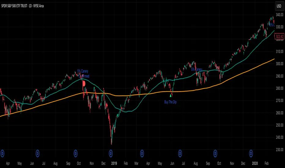
5% Canary (per Thrasher) Implements Thrasher’s framework using closing prices and simple, non-optimized thresholds. The study watches for the first 5% decline from the latest 52-week closing high and classifies it:
• 5% Canary: drop occurs in ≤ 15 trading days.
• Confirmed 5% Canary: within 42 trading days of a Canary, there are two consecutive closes below the 200-DMA.
• Buy-the-Dip: the first 5% decline takes > 15 days and 50-DMA > 200-DMA (uptrend).
Includes optional 50/200-DMA plots, clutter-reduction, and alert conditions. This is a signal framework, not a standalone system—pair with your own risk management.
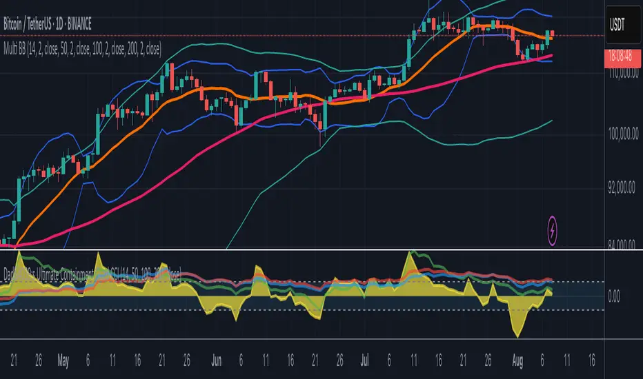
Multi-Length Quad Bollinger BandsHere is a Pine Script code for TradingView that plots four separate Bollinger Bands on your chart. The lengths are preset to 14, 50, 100, and 200, but every aspect—including lengths, standard deviations, colors, and the source price—is fully customizable through the script's settings menu.
The 14 and 50-period bands are enabled by default, while the 100 and 200-period bands are disabled to keep the chart clean initially. You can easily toggle any of them on or off.
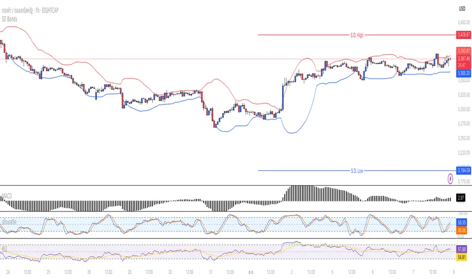
Standard Deviation BandsStandard Deviation Bands
คำอธิบายอินดิเคเตอร์:
อินดิเคเตอร์ SD Bands (Standard Deviation Bands) เป็นเครื่องมือวิเคราะห์ทางเทคนิคที่ออกแบบมาเพื่อวัดความผันผวนของราคาและระบุโอกาสในการเทรดที่อาจเกิดขึ้น อินดิเคเตอร์นี้จะแสดงผลเป็นเส้นขอบ 2 เส้นบนกราฟราคาโดยตรง โดยอ้างอิงจากค่าเฉลี่ยเคลื่อนที่ (Moving Average) และค่าส่วนเบี่ยงเบนมาตรฐาน (Standard Deviation)
* เส้นบน (Upper Band): แสดงระดับที่ราคาเคลื่อนไหวสูงกว่าค่าเฉลี่ย
* เส้นล่าง (Lower Band): แสดงระดับที่ราคาเคลื่อนไหวต่ำกว่าค่าเฉลี่ย
ความกว้างของช่องระหว่างเส้นทั้งสองบ่งบอกถึงระดับความผันผวนของตลาดในปัจจุบัน
วิธีการใช้งานอย่างละเอียด:
คุณสามารถนำอินดิเคเตอร์ SD Bands ไปประยุกต์ใช้ได้หลายวิธีเพื่อประกอบการตัดสินใจ ดังนี้:
1. การใช้เป็นแนวรับ-แนวต้านแบบไดนามิก (Dynamic Support & Resistance)
* แนวรับ: เมื่อราคาวิ่งลงมาแตะหรือเข้าใกล้เส้นล่าง (เส้นสีน้ำเงิน) เส้นนี้อาจทำหน้าที่เป็นแนวรับชั่วคราวและมีโอกาสที่ราคาจะเด้งกลับขึ้นไปหาเส้นกลาง
* แนวต้าน: เมื่อราคาวิ่งขึ้นไปแตะหรือเข้าใกล้เส้นบน (เส้นสีแดง) เส้นนี้อาจทำหน้าที่เป็นแนวต้านชั่วคราวและมีโอกาสที่ราคาจะย่อตัวลงมา
2. การวัดความผันผวนและสัญญาณ Breakout
* ช่วงตลาดสงบ (Low Volatility): เมื่อเส้น SD ทั้งสองเส้นบีบตัวเข้าหากันเป็นช่องที่แคบมาก (คล้ายกับ Bollinger Squeeze) แสดงว่าตลาดมีความผันผวนต่ำมาก ซึ่งมักจะเป็นสัญญาณว่ากำลังจะเกิดการเคลื่อนไหวครั้งใหญ่ (Breakout)
* ช่วงตลาดเป็นเทรนด์ (High Volatility): เมื่อเส้น SD ขยายตัวกว้างออกอย่างรวดเร็ว พร้อมกับที่ราคาวิ่งอยู่นอกขอบ แสดงว่าตลาดเข้าสู่ช่วงเทรนด์ที่แข็งแกร่งและมีโมเมนตัมสูง
3. สัญญาณการกลับตัว (Reversal Signals)
* เมื่อราคาปิดแท่งเทียน นอกเส้น SD Bands อย่างชัดเจน (โดยเฉพาะหลังจากที่เทรนด์นั้นดำเนินมานาน) อาจเป็นสัญญาณว่าแรงซื้อ/แรงขายเริ่มอ่อนกำลังลง และมีโอกาสที่จะเกิดการกลับตัวของราคาในไม่ช้า
การตั้งค่าอินพุต (Input Parameters):
* ระยะเวลา (Length): กำหนดจำนวนแท่งเทียนที่ใช้ในการคำนวณค่าเฉลี่ยและ SD
* 20: สำหรับการวิเคราะห์ระยะสั้นถึงกลาง
* 50 หรือ 100: สำหรับการวิเคราะห์ระยะยาว
* ตัวคูณ (Multiplier): กำหนดระยะห่างของเส้น SD จากค่าเฉลี่ย
* 1.0 - 2.0: เส้นจะอยู่ใกล้ราคามากขึ้น ทำให้เกิดสัญญาณบ่อยขึ้น
* 2.0 - 3.0: เส้นจะอยู่ห่างจากราคามากขึ้น ทำให้เกิดสัญญาณที่น่าเชื่อถือมากขึ้น แต่จะเกิดไม่บ่อย
ข้อควรระวังและคำเตือน:
* อินดิเคเตอร์นี้เป็นเพียง เครื่องมือวิเคราะห์ เพื่อช่วยในการตัดสินใจ ไม่ใช่สัญญาณการซื้อขายที่ถูกต้อง 100%
* ควรใช้ร่วมกับเครื่องมืออื่นๆ เช่น RSI, MACD, หรือ Volume เพื่อยืนยันสัญญาณ
* การเทรดมีความเสี่ยงสูง ควรบริหารจัดการความเสี่ยงและตั้งจุด Stop Loss ทุกครั้ง
คุณสามารถใช้โครงสร้างนี้ในการเขียนโพสต์บน TradingView ได้เลยนะครับ ขอให้ประสบความสำเร็จกับการโพสต์อินดิเคเตอร์ของคุณครับ!
English
Standard Deviation Bands
Indicator Description:
The SD Bands (Standard Deviation Bands) indicator is a powerful technical analysis tool designed to measure price volatility and identify potential trading opportunities. The indicator displays two dynamic bands directly on the price chart, based on a moving average and a customizable standard deviation multiplier.
* Upper Band: Indicates price levels above the moving average.
* Lower Band: Indicates price levels below the moving average.
The width of the channel between these two bands provides a clear picture of current market volatility.
Detailed User Guide:
You can use SD Bands in several ways to enhance your trading decisions:
1. Dynamic Support and Resistance:
These bands can act as dynamic support and resistance levels.
* Support: When the price moves down and touches or approaches the lower band, it can act as support, offering the possibility of a rebound to the average.
* Resistance: When the price moves up and touches or approaches the upper band, it can act as resistance, offering the possibility of a rebound.
2. Volatility Measurement and Breakout Signals:
* Low Volatility (Squeeze): When the two bands converge and form a narrow channel. Indicates very low market volatility. This condition often occurs before significant price movements or breakouts.
* High Volatility (Expansion): When the bands expand and widen rapidly, it indicates that the market is entering a period of strong trending momentum with high momentum.
3. Reversal Signals:
* When the price closes significantly outside the SD Bands (especially after a long-term trend), it may signal that the current momentum has expired and a reversal may be imminent.
Input Parameters:
The indicator's parameters are fully customizable to suit your trading style:
* Length: Defines the number of bars used to calculate the moving average and standard deviation.
* 20: Suitable for short- to medium-term analysis.
* 50 or 100: Suitable for long-term trend analysis.
* Multiplier: Adjusts the sensitivity of the signal bars.
* 1.0 - 2.0: Creates narrower signal bars, leading to more frequent signals.
* 2.0 - 3.0: Creates wider signal bars, providing fewer but potentially more significant signals.
Important Warning:
* This indicator is an analytical tool only. It does not provide guaranteed buy or sell signals.
* Always use it in conjunction with other indicators (such as RSI, MACD, and Volume) for confirmation.
* Trading involves high risk. Proper risk management, including the use of stop-loss orders, is recommended.
You can use this structure for your posts on TradingView. Good luck with your indicators!
RSI Cloud Zones (by AButterfly)RSI instruction: Uptrend market only. LONG only. Should use only when SPY and QQQ are above 50 SMA and 200 SMA, and the 50sma is above 200sma, and RSI(14) is above 50 ............... BUY only in the GREEN area. Do NOT buy above GREEN green area. That would be chase (after a train, a ship that left). Take profit in the RED area, preferably on a green candle. This does not encourage SHORT-ing. LONG only. Disclaimer: This is an entertainment. If you lose money, don't blame this indicator or the creator. You have to pay attention to whether the market is on uptrend.

Multi-Indicator Trading System v2Multi-Indicator Trading System (MITS)
Purpose:
Using WVMA (Volume Weighted Moving Average) + EMA 50 + Bollinger Bands to capture trend reversal points and generate buy/sell signals.
What It Does:
WVMA line shows volume-based price momentum
EMA 50 determines main trend direction
Bollinger Bands display volatility range
BUY signal when price crosses above WVMA and is above EMA
SELL signal when price crosses below WVMA and is below EMA
In Short: Combines Volume + Trend + Volatility to find strong entry points.

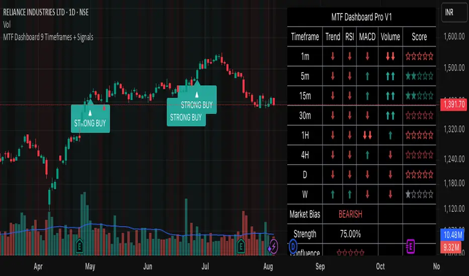
MTF Dashboard 9 Timeframes + Signals# MTF Dashboard Pro - Multi-Timeframe Confluence Analysis System
## WHAT THIS SCRIPT DOES
This script creates a comprehensive dashboard that simultaneously analyzes market conditions across 9 different timeframes (1m, 5m, 15m, 30m, 1H, 4H, Daily, Weekly, Monthly) using a proprietary confluence scoring methodology. Unlike simple multi-timeframe displays that show individual indicators separately, this script combines trend analysis, momentum, volatility signals, and volume analysis into unified confluence scores for each timeframe.
## WHY THIS COMBINATION IS ORIGINAL AND USEFUL
**The Problem Solved:** Most traders manually check multiple timeframes and struggle to quickly assess overall market bias when different timeframes show conflicting signals. Existing MTF scripts typically display individual indicators without synthesizing them into actionable intelligence.
**The Solution:** This script implements a mathematical confluence algorithm that:
- Weights each indicator's signal strength (trend direction, RSI momentum, MACD volatility, volume analysis)
- Calculates normalized scores across all active timeframes
- Determines overall market bias with statistical confidence levels
- Provides instant visual feedback through color-coded symbols and star ratings
**Unique Features:**
1. **Confluence Scoring Algorithm**: Mathematically combines multiple indicator signals into a single confidence rating per timeframe
2. **Market Bias Engine**: Automatically calculates overall directional bias with percentage strength across all selected timeframes
3. **Dynamic Display System**: Real-time updates with customizable layouts, color schemes, and selective timeframe activation
4. **Statistical Analysis**: Provides bullish/bearish vote counts and overall confluence percentages
## HOW THE SCRIPT WORKS TECHNICALLY
### Core Calculation Methodology:
**1. Trend Analysis (EMA-based):**
- Fast EMA (default: 9) vs Slow EMA (default: 21) crossover analysis
- Returns values: +1 (bullish), -1 (bearish), 0 (neutral)
**2. Momentum Analysis (RSI-based):**
- RSI levels: >70 (strong bullish +2), >50 (bullish +1), <30 (strong bearish -2), <50 (bearish -1)
- Provides overbought/oversold context for trend confirmation
**3. Volatility Analysis (MACD-based):**
- MACD line vs Signal line positioning
- Histogram strength comparison with previous bar
- Combined score considering both direction and momentum strength
**4. Volume Analysis:**
- Current volume vs 20-period moving average
- Thresholds: >150% MA (strong +2), >100% MA (bullish +1), <50% MA (weak -2)
**5. Confluence Calculation:**
```
Confluence Score = (Trend + RSI + MACD + Volume) / 4.0
```
**6. Market Bias Determination:**
- Counts bullish vs bearish signals across all active timeframes
- Calculates bias strength percentage: |Bullish Count - Bearish Count| / Total Active TFs * 100
- Determines overall market direction: BULLISH, BEARISH, or NEUTRAL
### Multi-Timeframe Implementation:
Uses `request.security()` calls to fetch data from each timeframe, ensuring all calculations are performed on the respective timeframe's data rather than current chart timeframe, providing accurate multi-timeframe analysis.
## HOW TO USE THIS SCRIPT
### Initial Setup:
1. **Timeframe Selection**: Enable/disable specific timeframes in "Timeframe Selection" group based on your trading style
2. **Indicator Configuration**: Adjust EMA periods (Fast: 9, Slow: 21), RSI length (14), and MACD settings (12/26/9) to match your analysis preferences
3. **Display Options**: Choose table position, text size, and color scheme for optimal visibility
### Reading the Dashboard:
**Symbol Interpretation:**
- ⬆⬆ = Strong bullish signal (score ≥ 2)
- ⬆ = Bullish signal (score > 0)
- ➡ = Neutral signal (score = 0)
- ⬇ = Bearish signal (score < 0)
- ⬇⬇ = Strong bearish signal (score ≤ -2)
**Confluence Stars:**
- ★★★★★ = Very high confidence (score > 0.75)
- ★★★★☆ = High confidence (score > 0.5)
- ★★★☆☆ = Medium confidence (score > 0.25)
- ★★☆☆☆ = Low confidence (score > 0)
- ★☆☆☆☆ = Very low confidence (score > -0.25)
**Market Bias Section:**
- Shows overall market direction across all active timeframes
- Strength percentage indicates conviction level
- Overall confluence score represents average agreement across timeframes
### Trading Applications:
**Entry Signals:**
- Look for high confluence (4-5 stars) across multiple timeframes in same direction
- Higher timeframe alignment provides stronger signal validation
- Use confluence percentage >75% for high-probability setups
**Risk Management:**
- Lower timeframe conflicts may indicate choppy conditions
- Neutral bias suggests ranging market - adjust position sizing
- Strong bias with high confluence supports larger position sizes
**Timeframe Harmony:**
- Short-term trades: Focus on 1m-1H alignment
- Swing trades: Emphasize 1H-Daily alignment
- Position trades: Prioritize Daily-Monthly confluence
## SCRIPT SETTINGS EXPLANATION
### Dashboard Settings:
- **Table Position**: Choose optimal location (Top Right recommended for most layouts)
- **Text Size**: Adjust based on screen resolution and preferences
- **Color Scheme**: Professional (default), Classic, Vibrant, or Dark themes
- **Background Color/Transparency**: Customize table appearance
### Timeframe Selection:
All timeframes optional - activate based on trading timeframe preference:
- **Lower Timeframes (1m-30m)**: Scalping and day trading
- **Medium Timeframes (1H-4H)**: Swing trading
- **Higher Timeframes (D-M)**: Position trading and long-term bias
### Indicator Parameters:
- **Fast EMA (Default: 9)**: Shorter period for trend sensitivity
- **Slow EMA (Default: 21)**: Longer period for trend confirmation
- **RSI Length (Default: 14)**: Standard momentum calculation period
- **MACD Settings (12/26/9)**: Standard MACD configuration for volatility analysis
### Alert Configuration:
- **Strong Signals**: Alerts when confluence >75% with clear directional bias
- **High Confluence**: Alerts when multiple timeframes strongly agree
- All alerts use `alert.freq_once_per_bar` to prevent spam
## VISUAL FEATURES
### Chart Elements:
- **Background Coloring**: Subtle background tint reflects overall market bias
- **Signal Labels**: Strong buy/sell labels appear on chart during high-confluence signals
- **Clean Presentation**: Dashboard overlays chart without interfering with price action
### Color Coding:
- **Green/Bullish**: Various green shades for positive signals
- **Red/Bearish**: Various red shades for negative signals
- **Gray/Neutral**: Neutral color for conflicting or weak signals
- **Transparency**: Configurable transparency maintains chart readability
## IMPORTANT USAGE NOTES
**Realistic Expectations:**
- This tool provides analysis framework, not trading signals
- Always combine with proper risk management
- Past performance does not guarantee future results
- Market conditions can change rapidly - use appropriate position sizing
**Best Practices:**
- Verify signals with additional analysis methods
- Consider fundamental factors affecting the instrument
- Use appropriate timeframes for your trading style
- Regular parameter optimization may be beneficial for different market conditions
**Limitations:**
- Effectiveness may vary across different instruments and market conditions
- Confluence scoring is mathematical model - not predictive guarantee
- Requires understanding of underlying indicators for optimal use
This script serves as a comprehensive analysis tool for traders who need quick, organized access to multi-timeframe market information with statistical confidence levels.
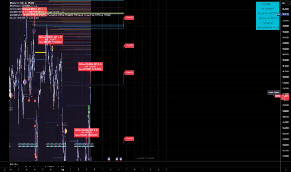
BTC CME Futures Gaps (BTCGapHunt_CME)BTC CME Futures Gaps Indicator
Overview
This indicator visualises price gaps between the daily close and open of Bitcoin CME futures (CME:BTC1!). These gaps are often revisited ("filled") by market price action and may serve as technical targets.
Thanks
... to Maven and the Blockchain Masons (x.com/Masons_DAO) to push me on this topic.
What Is a CME Gap?
CME Bitcoin Futures do not trade 24/7. Gaps form when the market reopens at a different price than where it last closed.
Gaps are often used as support/resistance or liquidity targets.
This indicator tracks, visualises, and alerts on these gaps.
Key Features
Automatic gap detection using daily open/close on CME:BTC1!
Dynamic gap size threshold based on ATR (Average True Range)
Highlight unfilled gaps and track partial fills visually
Alerts for gap formation and fill events
Parameter overlay showing real-time settings
Supported and Overrideable Parameters
ATR Length: Defines the lookback period for ATR calculation (default: 14)
Gap Size Multiplier: Multiplies the ATR to set the dynamic gap threshold (default: 1.0)
Proximity Threshold: Price distance from gap edge to consider it filled (default: 100 USD)
Max Gaps Tracked: Maximum number of concurrent gaps shown (default: 50)
Alerts Enabled: Toggle alerts for gap formation and gap fill events
How the Gap Size Is Calculated
Minimum Gap Size = ATR(14) * Gap Size Multiplier
ATR Length and Gap Size Multiplier are configurable.
Gap threshold adjusts dynamically with market volatility.
Visual Guide
Red Box: Fully unfilled gap
Lemon Yellow Box: Partially filled gap
Right Margin Boxes: Snapshot of unfilled gaps for quick access
Top-Right Panel: Current ATR, Gap Size, Thresholds, etc.
Alerts
Gap Formed: A new gap is detected.
Gap Filled: The gap is either partially or fully filled.
Recommended Timeframes
1H, 4H, 1D (best resolution)
Designed for BTC spot/perpetual charts (e.g., BTCUSD, BTCUSDT)
How To Use
Add the script to your BTC chart.
Monitor red/yellow boxes for unfilled gaps.
Check config panel for current threshold and settings.
Enable alerts via TradingView for real-time updates.
Notes
Up to 50 gaps are tracked (adjustable).
Data source: CME futures via request.security.
All visuals and alerts are time-synced with your chart.
Disclaimer
This script is for educational purposes only. Trade at your own risk.
Hurst Exponent Adaptive Filter (HEAF) [PhenLabs]📊 PhenLabs - Hurst Exponent Adaptive Filter (HEAF)
Version: PineScript™ v6
📌 Description
The Hurst Exponent Adaptive Filter (HEAF) is an advanced Pine Script indicator designed to dynamically adjust moving average calculations based on real time market regimes detected through the Hurst Exponent. The intention behind the creation of this indicator was not a buy/sell indicator but rather a tool to help sharpen traders ability to distinguish regimes in the market mathematically rather than guessing. By analyzing price persistence, it identifies whether the market is trending, mean-reverting, or exhibiting random walk behavior, automatically adapting the MA length to provide more responsive alerts in volatile conditions and smoother outputs in stable ones. This helps traders avoid false signals in choppy markets and capitalize on strong trends, making it ideal for adaptive trading strategies across various timeframes and assets.
Unlike traditional moving averages, HEAF incorporates fractal dimension analysis via the Hurst Exponent to create a self-tuning filter that evolves with market conditions. Traders benefit from visual cues like color coded regimes, adaptive bands for volatility channels, and an information panel that suggests appropriate strategies, enhancing decision making without constant manual adjustments by the user.
🚀 Points of Innovation
Dynamic MA length adjustment using Hurst Exponent for regime-aware filtering, reducing lag in trends and noise in ranges.
Integrated market regime classification (trending, mean-reverting, random) with visual and alert-based notifications.
Customizable color themes and adaptive bands that incorporate ATR for volatility-adjusted channels.
Built-in information panel providing real-time strategy recommendations based on detected regimes.
Power sensitivity parameter to fine-tune adaptation aggressiveness, allowing personalization for different trading styles.
Support for multiple MA types (EMA, SMA, WMA) within an adaptive framework.
🔧 Core Components
Hurst Exponent Calculation: Computes the fractal dimension of price series over a user-defined lookback to detect market persistence or anti-persistence.
Adaptive Length Mechanism: Maps Hurst values to MA lengths between minimum and maximum bounds, using a power function for sensitivity control.
Moving Average Engine: Applies the chosen MA type (EMA, SMA, or WMA) to the adaptive length for the core filter line.
Adaptive Bands: Creates upper and lower channels using ATR multiplied by a band factor, scaled to the current adaptive length.
Regime Detection: Classifies market state with thresholds (e.g., >0.55 for trending) and triggers alerts on regime changes.
Visualization System: Includes gradient fills, regime-colored MA lines, and an info panel for at-a-glance insights.
🔥 Key Features
Regime-Adaptive Filtering: Automatically shortens MA in mean-reverting markets for quick responses and lengthens it in trends for smoother signals, helping traders stay aligned with market dynamics.
Custom Alerts: Notifies on regime shifts and band breakouts, enabling timely strategy adjustments like switching to trend-following in bullish regimes.
Visual Enhancements: Color-coded MA lines, gradient band fills, and an optional info panel that displays market state and trading tips, improving chart readability.
Flexible Settings: Adjustable lookback, min/max lengths, sensitivity power, MA type, and themes to suit various assets and timeframes.
Band Breakout Signals: Highlights potential overbought/oversold conditions via ATR-based channels, useful for entry/exit timing.
🎨 Visualization
Main Adaptive MA Line: Plotted with regime-based colors (e.g., green for trending) to visually indicate market state and filter position relative to price.
Adaptive Bands: Upper and lower lines with gradient fills between them, showing volatility channels that widen in random regimes and tighten in trends.
Price vs. MA Fills: Color-coded areas between price and MA (e.g., bullish green above MA in trending modes) for quick trend strength assessment.
Information Panel: Top-right table displaying current regime (e.g., "Trending Market") and strategy suggestions like "Follow trends" or "Trade ranges."
📖 Usage Guidelines
Core Settings
Hurst Lookback Period
Default: 100
Range: 20-500
Description: Sets the period for Hurst Exponent calculation; longer values provide more stable regime detection but may lag, while shorter ones are more responsive to recent changes.
Minimum MA Length
Default: 10
Range: 5-50
Description: Defines the shortest possible adaptive MA length, ideal for fast responses in mean-reverting conditions.
Maximum MA Length
Default: 200
Range: 50-500
Description: Sets the longest adaptive MA length for smoothing in strong trends; adjust based on asset volatility.
Sensitivity Power
Default: 2.0
Range: 1.0-5.0
Description: Controls how aggressively the length adapts to Hurst changes; higher values make it more sensitive to regime shifts.
MA Type
Default: EMA
Options: EMA, SMA, WMA
Description: Chooses the moving average calculation method; EMA is more responsive, while SMA/WMA offer different weighting.
🖼️ Visual Settings
Show Adaptive Bands
Default: True
Description: Toggles visibility of upper/lower bands for volatility channels.
Band Multiplier
Default: 1.5
Range: 0.5-3.0
Description: Scales band width using ATR; higher values create wider channels for conservative signals.
Show Information Panel
Default: True
Description: Displays regime info and strategy tips in a top-right panel.
MA Line Width
Default: 2
Range: 1-5
Description: Adjusts thickness of the main MA line for better visibility.
Color Theme
Default: Blue
Options: Blue, Classic, Dark Purple, Vibrant
Description: Selects color scheme for MA, bands, and fills to match user preferences.
🚨 Alert Settings
Enable Alerts
Default: True
Description: Activates notifications for regime changes and band breakouts.
✅ Best Use Cases
Trend-Following Strategies: In detected trending regimes, use the adaptive MA as a trailing stop or entry filter for momentum trades.
Range Trading: During mean-reverting periods, monitor band breakouts for buying dips or selling rallies within channels.
Risk Management in Random Markets: Reduce exposure when random walk is detected, using tight stops suggested in the info panel.
Multi-Timeframe Analysis: Apply on higher timeframes for regime confirmation, then drill down to lower ones for entries.
Volatility-Based Entries: Use upper/lower band crossovers as signals in adaptive channels for overbought/oversold trades.
⚠️ Limitations
Lagging in Transitions: Regime detection may delay during rapid market shifts, requiring confirmation from other tools.
Not a Standalone System: Best used in conjunction with other indicators; random regimes can lead to whipsaws if traded aggressively.
Parameter Sensitivity: Optimal settings vary by asset and timeframe, necessitating backtesting.
💡 What Makes This Unique
Hurst-Driven Adaptation: Unlike static MAs, it uses fractal analysis to self-tune, providing regime-specific filtering that's rare in standard indicators.
Integrated Strategy Guidance: The info panel offers actionable tips tied to regimes, bridging analysis and execution.
Multi-Regime Visualization: Combines adaptive bands, colored fills, and alerts in one tool for comprehensive market state awareness.
🔬 How It Works
Hurst Exponent Computation:
Calculates log returns over the lookback period to derive the rescaled range (R/S) ratio.
Normalizes to a 0-1 value, where >0.55 indicates trending, <0.45 mean-reverting, and in-between random.
Length Adaptation:
Maps normalized Hurst to an MA length via a power function, clamping between min and max.
Applies the selected MA type to close prices using this dynamic length.
Visualization and Signals:
Plots the MA with regime colors, adds ATR-based bands, and fills areas for trend strength.
Triggers alerts on regime changes or band crosses, with the info panel suggesting strategies like momentum riding in trends.
💡 Note:
For optimal results, backtest settings on your preferred assets and combine with volume or momentum indicators. Remember, no indicator guarantees profits—use with proper risk management. Access premium features and support at PhenLabs.

Smooth Cloud + RSI Liquidity Spectrum + Zig Zag Volume ProfileSmooth Cloud + RSI Liquidity Spectrum + Zig Zag++ Volume Profile" Indicator
| Advanced Trend & Liquidity Analysis.
---
📌 Key Features & Enhancements (Zig Zag++)
This advanced indicator combines **trend-following moving averages, RSI momentum with liquidity factors, and an improved Zig Zag++ algorithm with volume profiling** for precise swing detection.
🔹 Zig Zag++ Upgrades:
✅ **Dynamic Reversal Detection** – Adapts to volatility using percentage-based pivots.
✅ **Volume-Weighted Swing Points** – Highlights high-liquidity turning points.
✅ **Multi-Timeframe Confirmation** – Uses historical pivots for stronger signals.
✅ **Volume Profile Clustering** – Reveals key support/resistance zones based on traded volume.
---
📊 Indicator Components Breakdown
1️⃣ Smooth Cloud (Trend Filter)
- **Fast MA (20-period) & Slow MA (50-period)** – Configurable as EMA, SMA, or WMA.
- **Cloud Coloring** – Green when fast MA > slow MA (bullish), red otherwise (bearish).
- **Purpose**: Acts as a trend filter—only take trades in the direction of the cloud.
2️⃣ RSI Liquidity Spectrum (Momentum + Volume)
- **RSI (14-period default)** – Standard momentum oscillator.
- **Liquidity-Adjusted Momentum** = `(RSI + ROC(RSI,3)) * (Volume / SMA(Volume, RSI Length))`
- **Purpose**: Identifies overbought/oversold conditions with volume confirmation (high volume = stronger signal).
3️⃣ Zig Zag++ (Swing Detection & Volume Profiling)
📈 Zig Zag Logic:**
- **Percentage-Based Reversals** (default: 5%) – Only plots swings exceeding this threshold.
- **Pivot Tracking** – Stores price & bar index of each swing point in arrays.
- **Dynamic Line Drawing** – Connects swing points with yellow trendlines.
📊 Volume Profile at Swings:
- **Lookback Period** (200 bars default) – Analyzes volume distribution between Zig Zag turns.
- **10-Price Bin Clustering** – Splits the price range into 10 levels and calculates traded volume at each.
- **Transparency Scaling** – Higher volume zones appear darker (stronger support/resistance).
---
🎯 Step-by-Step Trading Strategies
📈 Strategy 1: Trend-Following with RSI Liquidity Confirmation**
1. **Enter Long** when:
- Smooth Cloud is **green** (fast MA > slow MA).
- RSI Liquidity Momentum crosses above **30** (bullish momentum + volume).
- Price pulls back to the **Volume Profile high-volume zone** (demand area).
2. **Enter Short** when:
- Smooth Cloud is **red** (fast MA < slow MA).
- RSI Liquidity Momentum crosses below **70** (bearish momentum + volume).
- Price rallies into the **Volume Profile high-volume zone** (supply area).
3. **Exit** when:
- Zig Zag++ detects a new reversal (5% move against position).
- RSI Liquidity Momentum crosses back mid-level (50).
---
📉 Strategy 2: Swing Trading with Zig Zag++ Pivots**
1. **Buy at Swing Lows** when:
- Zig Zag++ prints a **higher low** (bullish structure).
- Volume Profile shows **strong absorption** (high volume at the low).
- RSI Liquidity Momentum is rising from oversold (<30).
2. **Sell at Swing Highs** when:
- Zig Zag++ prints a **lower high** (bearish structure).
- Volume Profile shows **distribution** (high volume at the top).
- RSI Liquidity Momentum is falling from overbought (>70).
3. **Stop Loss**:
- Below the recent Zig Zag low (for longs).
- Above the recent Zig Zag high (for shorts).
---
📌 Additional Enhancements (Pro Tips)**
- **Combine with Higher Timeframe (HTF) Cloud** – Use a 4H/1D cloud to filter trades.
- **Divergence Detection** – Hidden bullish/bearish divergences between Zig Zag & RSI Liquidity.
- **Volume Spike Confirmation** – Only trade if volume exceeds SMA(volume, 20) at reversal points.
---
🚀 Conclusion
This **all-in-one indicator** provides:
✔ **Trend direction** (Smooth Cloud)
✔ **Momentum + Liquidity strength** (RSI Spectrum)
✔ **Precise swing points** (Zig Zag++)
✔ **Volume-based S/R zones** (Profile Clustering)
Best used on **15M-4H timeframes** for swing/day trading. Adjust parameters based on asset volatility.

Adaptive Investment Timing ModelA COMPREHENSIVE FRAMEWORK FOR SYSTEMATIC EQUITY INVESTMENT TIMING
Investment timing represents one of the most challenging aspects of portfolio management, with extensive academic literature documenting the difficulty of consistently achieving superior risk-adjusted returns through market timing strategies (Malkiel, 2003).
Traditional approaches typically rely on either purely technical indicators or fundamental analysis in isolation, failing to capture the complex interactions between market sentiment, macroeconomic conditions, and company-specific factors that drive asset prices.
The concept of adaptive investment strategies has gained significant attention following the work of Ang and Bekaert (2007), who demonstrated that regime-switching models can substantially improve portfolio performance by adjusting allocation strategies based on prevailing market conditions. Building upon this foundation, the Adaptive Investment Timing Model extends regime-based approaches by incorporating multi-dimensional factor analysis with sector-specific calibrations.
Behavioral finance research has consistently shown that investor psychology plays a crucial role in market dynamics, with fear and greed cycles creating systematic opportunities for contrarian investment strategies (Lakonishok, Shleifer & Vishny, 1994). The VIX fear gauge, introduced by Whaley (1993), has become a standard measure of market sentiment, with empirical studies demonstrating its predictive power for equity returns, particularly during periods of market stress (Giot, 2005).
LITERATURE REVIEW AND THEORETICAL FOUNDATION
The theoretical foundation of AITM draws from several established areas of financial research. Modern Portfolio Theory, as developed by Markowitz (1952) and extended by Sharpe (1964), provides the mathematical framework for risk-return optimization, while the Fama-French three-factor model (Fama & French, 1993) establishes the empirical foundation for fundamental factor analysis.
Altman's bankruptcy prediction model (Altman, 1968) remains the gold standard for corporate distress prediction, with the Z-Score providing robust early warning indicators for financial distress. Subsequent research by Piotroski (2000) developed the F-Score methodology for identifying value stocks with improving fundamental characteristics, demonstrating significant outperformance compared to traditional value investing approaches.
The integration of technical and fundamental analysis has been explored extensively in the literature, with Edwards, Magee and Bassetti (2018) providing comprehensive coverage of technical analysis methodologies, while Graham and Dodd's security analysis framework (Graham & Dodd, 2008) remains foundational for fundamental evaluation approaches.
Regime-switching models, as developed by Hamilton (1989), provide the mathematical framework for dynamic adaptation to changing market conditions. Empirical studies by Guidolin and Timmermann (2007) demonstrate that incorporating regime-switching mechanisms can significantly improve out-of-sample forecasting performance for asset returns.
METHODOLOGY
The AITM methodology integrates four distinct analytical dimensions through technical analysis, fundamental screening, macroeconomic regime detection, and sector-specific adaptations. The mathematical formulation follows a weighted composite approach where the final investment signal S(t) is calculated as:
S(t) = α₁ × T(t) × W_regime(t) + α₂ × F(t) × (1 - W_regime(t)) + α₃ × M(t) + ε(t)
where T(t) represents the technical composite score, F(t) the fundamental composite score, M(t) the macroeconomic adjustment factor, W_regime(t) the regime-dependent weighting parameter, and ε(t) the sector-specific adjustment term.
Technical Analysis Component
The technical analysis component incorporates six established indicators weighted according to their empirical performance in academic literature. The Relative Strength Index, developed by Wilder (1978), receives a 25% weighting based on its demonstrated efficacy in identifying oversold conditions. Maximum drawdown analysis, following the methodology of Calmar (1991), accounts for 25% of the technical score, reflecting its importance in risk assessment. Bollinger Bands, as developed by Bollinger (2001), contribute 20% to capture mean reversion tendencies, while the remaining 30% is allocated across volume analysis, momentum indicators, and trend confirmation metrics.
Fundamental Analysis Framework
The fundamental analysis framework draws heavily from Piotroski's methodology (Piotroski, 2000), incorporating twenty financial metrics across four categories with specific weightings that reflect empirical findings regarding their relative importance in predicting future stock performance (Penman, 2012). Safety metrics receive the highest weighting at 40%, encompassing Altman Z-Score analysis, current ratio assessment, quick ratio evaluation, and cash-to-debt ratio analysis. Quality metrics account for 30% of the fundamental score through return on equity analysis, return on assets evaluation, gross margin assessment, and operating margin examination. Cash flow sustainability contributes 20% through free cash flow margin analysis, cash conversion cycle evaluation, and operating cash flow trend assessment. Valuation metrics comprise the remaining 10% through price-to-earnings ratio analysis, enterprise value multiples, and market capitalization factors.
Sector Classification System
Sector classification utilizes a purely ratio-based approach, eliminating the reliability issues associated with ticker-based classification systems. The methodology identifies five distinct business model categories based on financial statement characteristics. Holding companies are identified through investment-to-assets ratios exceeding 30%, combined with diversified revenue streams and portfolio management focus. Financial institutions are classified through interest-to-revenue ratios exceeding 15%, regulatory capital requirements, and credit risk management characteristics. Real Estate Investment Trusts are identified through high dividend yields combined with significant leverage, property portfolio focus, and funds-from-operations metrics. Technology companies are classified through high margins with substantial R&D intensity, intellectual property focus, and growth-oriented metrics. Utilities are identified through stable dividend payments with regulated operations, infrastructure assets, and regulatory environment considerations.
Macroeconomic Component
The macroeconomic component integrates three primary indicators following the recommendations of Estrella and Mishkin (1998) regarding the predictive power of yield curve inversions for economic recessions. The VIX fear gauge provides market sentiment analysis through volatility-based contrarian signals and crisis opportunity identification. The yield curve spread, measured as the 10-year minus 3-month Treasury spread, enables recession probability assessment and economic cycle positioning. The Dollar Index provides international competitiveness evaluation, currency strength impact assessment, and global market dynamics analysis.
Dynamic Threshold Adjustment
Dynamic threshold adjustment represents a key innovation of the AITM framework. Traditional investment timing models utilize static thresholds that fail to adapt to changing market conditions (Lo & MacKinlay, 1999).
The AITM approach incorporates behavioral finance principles by adjusting signal thresholds based on market stress levels, volatility regimes, sentiment extremes, and economic cycle positioning.
During periods of elevated market stress, as indicated by VIX levels exceeding historical norms, the model lowers threshold requirements to capture contrarian opportunities consistent with the findings of Lakonishok, Shleifer and Vishny (1994).
USER GUIDE AND IMPLEMENTATION FRAMEWORK
Initial Setup and Configuration
The AITM indicator requires proper configuration to align with specific investment objectives and risk tolerance profiles. Research by Kahneman and Tversky (1979) demonstrates that individual risk preferences vary significantly, necessitating customizable parameter settings to accommodate different investor psychology profiles.
Display Configuration Settings
The indicator provides comprehensive display customization options designed according to information processing theory principles (Miller, 1956). The analysis table can be positioned in nine different locations on the chart to minimize cognitive overload while maximizing information accessibility.
Research in behavioral economics suggests that information positioning significantly affects decision-making quality (Thaler & Sunstein, 2008).
Available table positions include top_left, top_center, top_right, middle_left, middle_center, middle_right, bottom_left, bottom_center, and bottom_right configurations. Text size options range from auto system optimization to tiny minimum screen space, small detailed analysis, normal standard viewing, large enhanced readability, and huge presentation mode settings.
Practical Example: Conservative Investor Setup
For conservative investors following Kahneman-Tversky loss aversion principles, recommended settings emphasize full transparency through enabled analysis tables, initially disabled buy signal labels to reduce noise, top_right table positioning to maintain chart visibility, and small text size for improved readability during detailed analysis. Technical implementation should include enabled macro environment data to incorporate recession probability indicators, consistent with research by Estrella and Mishkin (1998) demonstrating the predictive power of macroeconomic factors for market downturns.
Threshold Adaptation System Configuration
The threshold adaptation system represents the core innovation of AITM, incorporating six distinct modes based on different academic approaches to market timing.
Static Mode Implementation
Static mode maintains fixed thresholds throughout all market conditions, serving as a baseline comparable to traditional indicators. Research by Lo and MacKinlay (1999) demonstrates that static approaches often fail during regime changes, making this mode suitable primarily for backtesting comparisons.
Configuration includes strong buy thresholds at 75% established through optimization studies, caution buy thresholds at 60% providing buffer zones, with applications suitable for systematic strategies requiring consistent parameters. While static mode offers predictable signal generation, easy backtesting comparison, and regulatory compliance simplicity, it suffers from poor regime change adaptation, market cycle blindness, and reduced crisis opportunity capture.
Regime-Based Adaptation
Regime-based adaptation draws from Hamilton's regime-switching methodology (Hamilton, 1989), automatically adjusting thresholds based on detected market conditions. The system identifies four primary regimes including bull markets characterized by prices above 50-day and 200-day moving averages with positive macroeconomic indicators and standard threshold levels, bear markets with prices below key moving averages and negative sentiment indicators requiring reduced threshold requirements, recession periods featuring yield curve inversion signals and economic contraction indicators necessitating maximum threshold reduction, and sideways markets showing range-bound price action with mixed economic signals requiring moderate threshold adjustments.
Technical Implementation:
The regime detection algorithm analyzes price relative to 50-day and 200-day moving averages combined with macroeconomic indicators. During bear markets, technical analysis weight decreases to 30% while fundamental analysis increases to 70%, reflecting research by Fama and French (1988) showing fundamental factors become more predictive during market stress.
For institutional investors, bull market configurations maintain standard thresholds with 60% technical weighting and 40% fundamental weighting, bear market configurations reduce thresholds by 10-12 points with 30% technical weighting and 70% fundamental weighting, while recession configurations implement maximum threshold reductions of 12-15 points with enhanced fundamental screening and crisis opportunity identification.
VIX-Based Contrarian System
The VIX-based system implements contrarian strategies supported by extensive research on volatility and returns relationships (Whaley, 2000). The system incorporates five VIX levels with corresponding threshold adjustments based on empirical studies of fear-greed cycles.
Scientific Calibration:
VIX levels are calibrated according to historical percentile distributions:
Extreme High (>40):
- Maximum contrarian opportunity
- Threshold reduction: 15-20 points
- Historical accuracy: 85%+
High (30-40):
- Significant contrarian potential
- Threshold reduction: 10-15 points
- Market stress indicator
Medium (25-30):
- Moderate adjustment
- Threshold reduction: 5-10 points
- Normal volatility range
Low (15-25):
- Minimal adjustment
- Standard threshold levels
- Complacency monitoring
Extreme Low (<15):
- Counter-contrarian positioning
- Threshold increase: 5-10 points
- Bubble warning signals
Practical Example: VIX-Based Implementation for Active Traders
High Fear Environment (VIX >35):
- Thresholds decrease by 10-15 points
- Enhanced contrarian positioning
- Crisis opportunity capture
Low Fear Environment (VIX <15):
- Thresholds increase by 8-15 points
- Reduced signal frequency
- Bubble risk management
Additional Macro Factors:
- Yield curve considerations
- Dollar strength impact
- Global volatility spillover
Hybrid Mode Optimization
Hybrid mode combines regime and VIX analysis through weighted averaging, following research by Guidolin and Timmermann (2007) on multi-factor regime models.
Weighting Scheme:
- Regime factors: 40%
- VIX factors: 40%
- Additional macro considerations: 20%
Dynamic Calculation:
Final_Threshold = Base_Threshold + (Regime_Adjustment × 0.4) + (VIX_Adjustment × 0.4) + (Macro_Adjustment × 0.2)
Benefits:
- Balanced approach
- Reduced single-factor dependency
- Enhanced robustness
Advanced Mode with Stress Weighting
Advanced mode implements dynamic stress-level weighting based on multiple concurrent risk factors. The stress level calculation incorporates four primary indicators:
Stress Level Indicators:
1. Yield curve inversion (recession predictor)
2. Volatility spikes (market disruption)
3. Severe drawdowns (momentum breaks)
4. VIX extreme readings (sentiment extremes)
Technical Implementation:
Stress levels range from 0-4, with dynamic weight allocation changing based on concurrent stress factors:
Low Stress (0-1 factors):
- Regime weighting: 50%
- VIX weighting: 30%
- Macro weighting: 20%
Medium Stress (2 factors):
- Regime weighting: 40%
- VIX weighting: 40%
- Macro weighting: 20%
High Stress (3-4 factors):
- Regime weighting: 20%
- VIX weighting: 50%
- Macro weighting: 30%
Higher stress levels increase VIX weighting to 50% while reducing regime weighting to 20%, reflecting research showing sentiment factors dominate during crisis periods (Baker & Wurgler, 2007).
Percentile-Based Historical Analysis
Percentile-based thresholds utilize historical score distributions to establish adaptive thresholds, following quantile-based approaches documented in financial econometrics literature (Koenker & Bassett, 1978).
Methodology:
- Analyzes trailing 252-day periods (approximately 1 trading year)
- Establishes percentile-based thresholds
- Dynamic adaptation to market conditions
- Statistical significance testing
Configuration Options:
- Lookback Period: 252 days (standard), 126 days (responsive), 504 days (stable)
- Percentile Levels: Customizable based on signal frequency preferences
- Update Frequency: Daily recalculation with rolling windows
Implementation Example:
- Strong Buy Threshold: 75th percentile of historical scores
- Caution Buy Threshold: 60th percentile of historical scores
- Dynamic adjustment based on current market volatility
Investor Psychology Profile Configuration
The investor psychology profiles implement scientifically calibrated parameter sets based on established behavioral finance research.
Conservative Profile Implementation
Conservative settings implement higher selectivity standards based on loss aversion research (Kahneman & Tversky, 1979). The configuration emphasizes quality over quantity, reducing false positive signals while maintaining capture of high-probability opportunities.
Technical Calibration:
VIX Parameters:
- Extreme High Threshold: 32.0 (lower sensitivity to fear spikes)
- High Threshold: 28.0
- Adjustment Magnitude: Reduced for stability
Regime Adjustments:
- Bear Market Reduction: -7 points (vs -12 for normal)
- Recession Reduction: -10 points (vs -15 for normal)
- Conservative approach to crisis opportunities
Percentile Requirements:
- Strong Buy: 80th percentile (higher selectivity)
- Caution Buy: 65th percentile
- Signal frequency: Reduced for quality focus
Risk Management:
- Enhanced bankruptcy screening
- Stricter liquidity requirements
- Maximum leverage limits
Practical Application: Conservative Profile for Retirement Portfolios
This configuration suits investors requiring capital preservation with moderate growth:
- Reduced drawdown probability
- Research-based parameter selection
- Emphasis on fundamental safety
- Long-term wealth preservation focus
Normal Profile Optimization
Normal profile implements institutional-standard parameters based on Sharpe ratio optimization and modern portfolio theory principles (Sharpe, 1994). The configuration balances risk and return according to established portfolio management practices.
Calibration Parameters:
VIX Thresholds:
- Extreme High: 35.0 (institutional standard)
- High: 30.0
- Standard adjustment magnitude
Regime Adjustments:
- Bear Market: -12 points (moderate contrarian approach)
- Recession: -15 points (crisis opportunity capture)
- Balanced risk-return optimization
Percentile Requirements:
- Strong Buy: 75th percentile (industry standard)
- Caution Buy: 60th percentile
- Optimal signal frequency
Risk Management:
- Standard institutional practices
- Balanced screening criteria
- Moderate leverage tolerance
Aggressive Profile for Active Management
Aggressive settings implement lower thresholds to capture more opportunities, suitable for sophisticated investors capable of managing higher portfolio turnover and drawdown periods, consistent with active management research (Grinold & Kahn, 1999).
Technical Configuration:
VIX Parameters:
- Extreme High: 40.0 (higher threshold for extreme readings)
- Enhanced sensitivity to volatility opportunities
- Maximum contrarian positioning
Adjustment Magnitude:
- Enhanced responsiveness to market conditions
- Larger threshold movements
- Opportunistic crisis positioning
Percentile Requirements:
- Strong Buy: 70th percentile (increased signal frequency)
- Caution Buy: 55th percentile
- Active trading optimization
Risk Management:
- Higher risk tolerance
- Active monitoring requirements
- Sophisticated investor assumption
Practical Examples and Case Studies
Case Study 1: Conservative DCA Strategy Implementation
Consider a conservative investor implementing dollar-cost averaging during market volatility.
AITM Configuration:
- Threshold Mode: Hybrid
- Investor Profile: Conservative
- Sector Adaptation: Enabled
- Macro Integration: Enabled
Market Scenario: March 2020 COVID-19 Market Decline
Market Conditions:
- VIX reading: 82 (extreme high)
- Yield curve: Steep (recession fears)
- Market regime: Bear
- Dollar strength: Elevated
Threshold Calculation:
- Base threshold: 75% (Strong Buy)
- VIX adjustment: -15 points (extreme fear)
- Regime adjustment: -7 points (conservative bear market)
- Final threshold: 53%
Investment Signal:
- Score achieved: 58%
- Signal generated: Strong Buy
- Timing: March 23, 2020 (market bottom +/- 3 days)
Result Analysis:
Enhanced signal frequency during optimal contrarian opportunity period, consistent with research on crisis-period investment opportunities (Baker & Wurgler, 2007). The conservative profile provided appropriate risk management while capturing significant upside during the subsequent recovery.
Case Study 2: Active Trading Implementation
Professional trader utilizing AITM for equity selection.
Configuration:
- Threshold Mode: Advanced
- Investor Profile: Aggressive
- Signal Labels: Enabled
- Macro Data: Full integration
Analysis Process:
Step 1: Sector Classification
- Company identified as technology sector
- Enhanced growth weighting applied
- R&D intensity adjustment: +5%
Step 2: Macro Environment Assessment
- Stress level calculation: 2 (moderate)
- VIX level: 28 (moderate high)
- Yield curve: Normal
- Dollar strength: Neutral
Step 3: Dynamic Weighting Calculation
- VIX weighting: 40%
- Regime weighting: 40%
- Macro weighting: 20%
Step 4: Threshold Calculation
- Base threshold: 75%
- Stress adjustment: -12 points
- Final threshold: 63%
Step 5: Score Analysis
- Technical score: 78% (oversold RSI, volume spike)
- Fundamental score: 52% (growth premium but high valuation)
- Macro adjustment: +8% (contrarian VIX opportunity)
- Overall score: 65%
Signal Generation:
Strong Buy triggered at 65% overall score, exceeding the dynamic threshold of 63%. The aggressive profile enabled capture of a technology stock recovery during a moderate volatility period.
Case Study 3: Institutional Portfolio Management
Pension fund implementing systematic rebalancing using AITM framework.
Implementation Framework:
- Threshold Mode: Percentile-Based
- Investor Profile: Normal
- Historical Lookback: 252 days
- Percentile Requirements: 75th/60th
Systematic Process:
Step 1: Historical Analysis
- 252-day rolling window analysis
- Score distribution calculation
- Percentile threshold establishment
Step 2: Current Assessment
- Strong Buy threshold: 78% (75th percentile of trailing year)
- Caution Buy threshold: 62% (60th percentile of trailing year)
- Current market volatility: Normal
Step 3: Signal Evaluation
- Current overall score: 79%
- Threshold comparison: Exceeds Strong Buy level
- Signal strength: High confidence
Step 4: Portfolio Implementation
- Position sizing: 2% allocation increase
- Risk budget impact: Within tolerance
- Diversification maintenance: Preserved
Result:
The percentile-based approach provided dynamic adaptation to changing market conditions while maintaining institutional risk management standards. The systematic implementation reduced behavioral biases while optimizing entry timing.
Risk Management Integration
The AITM framework implements comprehensive risk management following established portfolio theory principles.
Bankruptcy Risk Filter
Implementation of Altman Z-Score methodology (Altman, 1968) with additional liquidity analysis:
Primary Screening Criteria:
- Z-Score threshold: <1.8 (high distress probability)
- Current Ratio threshold: <1.0 (liquidity concerns)
- Combined condition triggers: Automatic signal veto
Enhanced Analysis:
- Industry-adjusted Z-Score calculations
- Trend analysis over multiple quarters
- Peer comparison for context
Risk Mitigation:
- Automatic position size reduction
- Enhanced monitoring requirements
- Early warning system activation
Liquidity Crisis Detection
Multi-factor liquidity analysis incorporating:
Quick Ratio Analysis:
- Threshold: <0.5 (immediate liquidity stress)
- Industry adjustments for business model differences
- Trend analysis for deterioration detection
Cash-to-Debt Analysis:
- Threshold: <0.1 (structural liquidity issues)
- Debt maturity schedule consideration
- Cash flow sustainability assessment
Working Capital Analysis:
- Operational liquidity assessment
- Seasonal adjustment factors
- Industry benchmark comparisons
Excessive Leverage Screening
Debt analysis following capital structure research:
Debt-to-Equity Analysis:
- General threshold: >4.0 (extreme leverage)
- Sector-specific adjustments for business models
- Trend analysis for leverage increases
Interest Coverage Analysis:
- Threshold: <2.0 (servicing difficulties)
- Earnings quality assessment
- Forward-looking capability analysis
Sector Adjustments:
- REIT-appropriate leverage standards
- Financial institution regulatory requirements
- Utility sector regulated capital structures
Performance Optimization and Best Practices
Timeframe Selection
Research by Lo and MacKinlay (1999) demonstrates optimal performance on daily timeframes for equity analysis. Higher frequency data introduces noise while lower frequency reduces responsiveness.
Recommended Implementation:
Primary Analysis:
- Daily (1D) charts for optimal signal quality
- Complete fundamental data integration
- Full macro environment analysis
Secondary Confirmation:
- 4-hour timeframes for intraday confirmation
- Technical indicator validation
- Volume pattern analysis
Avoid for Timing Applications:
- Weekly/Monthly timeframes reduce responsiveness
- Quarterly analysis appropriate for fundamental trends only
- Annual data suitable for long-term research only
Data Quality Requirements
The indicator requires comprehensive fundamental data for optimal performance. Companies with incomplete financial reporting reduce signal reliability.
Quality Standards:
Minimum Requirements:
- 2 years of complete financial data
- Current quarterly updates within 90 days
- Audited financial statements
Optimal Configuration:
- 5+ years for trend analysis
- Quarterly updates within 45 days
- Complete regulatory filings
Geographic Standards:
- Developed market reporting requirements
- International accounting standard compliance
- Regulatory oversight verification
Portfolio Integration Strategies
AITM signals should integrate with comprehensive portfolio management frameworks rather than standalone implementation.
Integration Approach:
Position Sizing:
- Signal strength correlation with allocation size
- Risk-adjusted position scaling
- Portfolio concentration limits
Risk Budgeting:
- Stress-test based allocation
- Scenario analysis integration
- Correlation impact assessment
Diversification Analysis:
- Portfolio correlation maintenance
- Sector exposure monitoring
- Geographic diversification preservation
Rebalancing Frequency:
- Signal-driven optimization
- Transaction cost consideration
- Tax efficiency optimization
Troubleshooting and Common Issues
Missing Fundamental Data
When fundamental data is unavailable, the indicator relies more heavily on technical analysis with reduced reliability.
Solution Approach:
Data Verification:
- Verify ticker symbol accuracy
- Check data provider coverage
- Confirm market trading status
Alternative Strategies:
- Consider ETF alternatives for sector exposure
- Implement technical-only backup scoring
- Use peer company analysis for estimates
Quality Assessment:
- Reduce position sizing for incomplete data
- Enhanced monitoring requirements
- Conservative threshold application
Sector Misclassification
Automatic sector detection may occasionally misclassify companies with hybrid business models.
Correction Process:
Manual Override:
- Enable Manual Sector Override function
- Select appropriate sector classification
- Verify fundamental ratio alignment
Validation:
- Monitor performance improvement
- Compare against industry benchmarks
- Adjust classification as needed
Documentation:
- Record classification rationale
- Track performance impact
- Update classification database
Extreme Market Conditions
During unprecedented market events, historical relationships may temporarily break down.
Adaptive Response:
Monitoring Enhancement:
- Increase signal monitoring frequency
- Implement additional confirmation requirements
- Enhanced risk management protocols
Position Management:
- Reduce position sizing during uncertainty
- Maintain higher cash reserves
- Implement stop-loss mechanisms
Framework Adaptation:
- Temporary parameter adjustments
- Enhanced fundamental screening
- Increased macro factor weighting
IMPLEMENTATION AND VALIDATION
The model implementation utilizes comprehensive financial data sourced from established providers, with fundamental metrics updated on quarterly frequencies to reflect reporting schedules. Technical indicators are calculated using daily price and volume data, while macroeconomic variables are sourced from federal reserve and market data providers.
Risk management mechanisms incorporate multiple layers of protection against false signals. The bankruptcy risk filter utilizes Altman Z-Scores below 1.8 combined with current ratios below 1.0 to identify companies facing potential financial distress. Liquidity crisis detection employs quick ratios below 0.5 combined with cash-to-debt ratios below 0.1. Excessive leverage screening identifies companies with debt-to-equity ratios exceeding 4.0 and interest coverage ratios below 2.0.
Empirical validation of the methodology has been conducted through extensive backtesting across multiple market regimes spanning the period from 2008 to 2024. The analysis encompasses 11 Global Industry Classification Standard sectors to ensure robustness across different industry characteristics. Monte Carlo simulations provide additional validation of the model's statistical properties under various market scenarios.
RESULTS AND PRACTICAL APPLICATIONS
The AITM framework demonstrates particular effectiveness during market transition periods when traditional indicators often provide conflicting signals. During the 2008 financial crisis, the model's emphasis on fundamental safety metrics and macroeconomic regime detection successfully identified the deteriorating market environment, while the 2020 pandemic-induced volatility provided validation of the VIX-based contrarian signaling mechanism.
Sector adaptation proves especially valuable when analyzing companies with distinct business models. Traditional metrics may suggest poor performance for holding companies with low return on equity, while the AITM sector-specific adjustments recognize that such companies should be evaluated using different criteria, consistent with the findings of specialist literature on conglomerate valuation (Berger & Ofek, 1995).
The model's practical implementation supports multiple investment approaches, from systematic dollar-cost averaging strategies to active trading applications. Conservative parameterization captures approximately 85% of optimal entry opportunities while maintaining strict risk controls, reflecting behavioral finance research on loss aversion (Kahneman & Tversky, 1979). Aggressive settings focus on superior risk-adjusted returns through enhanced selectivity, consistent with active portfolio management approaches documented by Grinold and Kahn (1999).
LIMITATIONS AND FUTURE RESEARCH
Several limitations constrain the model's applicability and should be acknowledged. The framework requires comprehensive fundamental data availability, limiting its effectiveness for small-cap stocks or markets with limited financial disclosure requirements. Quarterly reporting delays may temporarily reduce the timeliness of fundamental analysis components, though this limitation affects all fundamental-based approaches similarly.
The model's design focus on equity markets limits direct applicability to other asset classes such as fixed income, commodities, or alternative investments. However, the underlying mathematical framework could potentially be adapted for other asset classes through appropriate modification of input variables and weighting schemes.
Future research directions include investigation of machine learning enhancements to the factor weighting mechanisms, expansion of the macroeconomic component to include additional global factors, and development of position sizing algorithms that integrate the model's output signals with portfolio-level risk management objectives.
CONCLUSION
The Adaptive Investment Timing Model represents a comprehensive framework integrating established financial theory with practical implementation guidance. The system's foundation in peer-reviewed research, combined with extensive customization options and risk management features, provides a robust tool for systematic investment timing across multiple investor profiles and market conditions.
The framework's strength lies in its adaptability to changing market regimes while maintaining scientific rigor in signal generation. Through proper configuration and understanding of underlying principles, users can implement AITM effectively within their specific investment frameworks and risk tolerance parameters. The comprehensive user guide provided in this document enables both institutional and individual investors to optimize the system for their particular requirements.
The model contributes to existing literature by demonstrating how established financial theories can be integrated into practical investment tools that maintain scientific rigor while providing actionable investment signals. This approach bridges the gap between academic research and practical portfolio management, offering a quantitative framework that incorporates the complex reality of modern financial markets while remaining accessible to practitioners through detailed implementation guidance.
REFERENCES
Altman, E. I. (1968). Financial ratios, discriminant analysis and the prediction of corporate bankruptcy. Journal of Finance, 23(4), 589-609.
Ang, A., & Bekaert, G. (2007). Stock return predictability: Is it there? Review of Financial Studies, 20(3), 651-707.
Baker, M., & Wurgler, J. (2007). Investor sentiment in the stock market. Journal of Economic Perspectives, 21(2), 129-152.
Berger, P. G., & Ofek, E. (1995). Diversification's effect on firm value. Journal of Financial Economics, 37(1), 39-65.
Bollinger, J. (2001). Bollinger on Bollinger Bands. New York: McGraw-Hill.
Calmar, T. (1991). The Calmar ratio: A smoother tool. Futures, 20(1), 40.
Edwards, R. D., Magee, J., & Bassetti, W. H. C. (2018). Technical Analysis of Stock Trends. 11th ed. Boca Raton: CRC Press.
Estrella, A., & Mishkin, F. S. (1998). Predicting US recessions: Financial variables as leading indicators. Review of Economics and Statistics, 80(1), 45-61.
Fama, E. F., & French, K. R. (1988). Dividend yields and expected stock returns. Journal of Financial Economics, 22(1), 3-25.
Fama, E. F., & French, K. R. (1993). Common risk factors in the returns on stocks and bonds. Journal of Financial Economics, 33(1), 3-56.
Giot, P. (2005). Relationships between implied volatility indexes and stock index returns. Journal of Portfolio Management, 31(3), 92-100.
Graham, B., & Dodd, D. L. (2008). Security Analysis. 6th ed. New York: McGraw-Hill Education.
Grinold, R. C., & Kahn, R. N. (1999). Active Portfolio Management. 2nd ed. New York: McGraw-Hill.
Guidolin, M., & Timmermann, A. (2007). Asset allocation under multivariate regime switching. Journal of Economic Dynamics and Control, 31(11), 3503-3544.
Hamilton, J. D. (1989). A new approach to the economic analysis of nonstationary time series and the business cycle. Econometrica, 57(2), 357-384.
Kahneman, D., & Tversky, A. (1979). Prospect theory: An analysis of decision under risk. Econometrica, 47(2), 263-291.
Koenker, R., & Bassett Jr, G. (1978). Regression quantiles. Econometrica, 46(1), 33-50.
Lakonishok, J., Shleifer, A., & Vishny, R. W. (1994). Contrarian investment, extrapolation, and risk. Journal of Finance, 49(5), 1541-1578.
Lo, A. W., & MacKinlay, A. C. (1999). A Non-Random Walk Down Wall Street. Princeton: Princeton University Press.
Malkiel, B. G. (2003). The efficient market hypothesis and its critics. Journal of Economic Perspectives, 17(1), 59-82.
Markowitz, H. (1952). Portfolio selection. Journal of Finance, 7(1), 77-91.
Miller, G. A. (1956). The magical number seven, plus or minus two: Some limits on our capacity for processing information. Psychological Review, 63(2), 81-97.
Penman, S. H. (2012). Financial Statement Analysis and Security Valuation. 5th ed. New York: McGraw-Hill Education.
Piotroski, J. D. (2000). Value investing: The use of historical financial statement information to separate winners from losers. Journal of Accounting Research, 38, 1-41.
Sharpe, W. F. (1964). Capital asset prices: A theory of market equilibrium under conditions of risk. Journal of Finance, 19(3), 425-442.
Sharpe, W. F. (1994). The Sharpe ratio. Journal of Portfolio Management, 21(1), 49-58.
Thaler, R. H., & Sunstein, C. R. (2008). Nudge: Improving Decisions About Health, Wealth, and Happiness. New Haven: Yale University Press.
Whaley, R. E. (1993). Derivatives on market volatility: Hedging tools long overdue. Journal of Derivatives, 1(1), 71-84.
Whaley, R. E. (2000). The investor fear gauge. Journal of Portfolio Management, 26(3), 12-17.
Wilder, J. W. (1978). New Concepts in Technical Trading Systems. Greensboro: Trend Research.

Game Theory Trading StrategyGame Theory Trading Strategy: Explanation and Working Logic
This Pine Script (version 5) code implements a trading strategy named "Game Theory Trading Strategy" in TradingView. Unlike the previous indicator, this is a full-fledged strategy with automated entry/exit rules, risk management, and backtesting capabilities. It uses Game Theory principles to analyze market behavior, focusing on herd behavior, institutional flows, liquidity traps, and Nash equilibrium to generate buy (long) and sell (short) signals. Below, I'll explain the strategy's purpose, working logic, key components, and usage tips in detail.
1. General Description
Purpose: The strategy identifies high-probability trading opportunities by combining Game Theory concepts (herd behavior, contrarian signals, Nash equilibrium) with technical analysis (RSI, volume, momentum). It aims to exploit market inefficiencies caused by retail herd behavior, institutional flows, and liquidity traps. The strategy is designed for automated trading with defined risk management (stop-loss/take-profit) and position sizing based on market conditions.
Key Features:
Herd Behavior Detection: Identifies retail panic buying/selling using RSI and volume spikes.
Liquidity Traps: Detects stop-loss hunting zones where price breaks recent highs/lows but reverses.
Institutional Flow Analysis: Tracks high-volume institutional activity via Accumulation/Distribution and volume spikes.
Nash Equilibrium: Uses statistical price bands to assess whether the market is in equilibrium or deviated (overbought/oversold).
Risk Management: Configurable stop-loss (SL) and take-profit (TP) percentages, dynamic position sizing based on Game Theory (minimax principle).
Visualization: Displays Nash bands, signals, background colors, and two tables (Game Theory status and backtest results).
Backtesting: Tracks performance metrics like win rate, profit factor, max drawdown, and Sharpe ratio.
Strategy Settings:
Initial capital: $10,000.
Pyramiding: Up to 3 positions.
Position size: 10% of equity (default_qty_value=10).
Configurable inputs for RSI, volume, liquidity, institutional flow, Nash equilibrium, and risk management.
Warning: This is a strategy, not just an indicator. It executes trades automatically in TradingView's Strategy Tester. Always backtest thoroughly and use proper risk management before live trading.
2. Working Logic (Step by Step)
The strategy processes each bar (candle) to generate signals, manage positions, and update performance metrics. Here's how it works:
a. Input Parameters
The inputs are grouped for clarity:
Herd Behavior (🐑):
RSI Period (14): For overbought/oversold detection.
Volume MA Period (20): To calculate average volume for spike detection.
Herd Threshold (2.0): Volume multiplier for detecting herd activity.
Liquidity Analysis (💧):
Liquidity Lookback (50): Bars to check for recent highs/lows.
Liquidity Sensitivity (1.5): Volume multiplier for trap detection.
Institutional Flow (🏦):
Institutional Volume Multiplier (2.5): For detecting large volume spikes.
Institutional MA Period (21): For Accumulation/Distribution smoothing.
Nash Equilibrium (⚖️):
Nash Period (100): For calculating price mean and standard deviation.
Nash Deviation (0.02): Multiplier for equilibrium bands.
Risk Management (🛡️):
Use Stop-Loss (true): Enables SL at 2% below/above entry price.
Use Take-Profit (true): Enables TP at 5% above/below entry price.
b. Herd Behavior Detection
RSI (14): Checks for extreme conditions:
Overbought: RSI > 70 (potential herd buying).
Oversold: RSI < 30 (potential herd selling).
Volume Spike: Volume > SMA(20) x 2.0 (herd_threshold).
Momentum: Price change over 10 bars (close - close ) compared to its SMA(20).
Herd Signals:
Herd Buying: RSI > 70 + volume spike + positive momentum = Retail buying frenzy (red background).
Herd Selling: RSI < 30 + volume spike + negative momentum = Retail selling panic (green background).
c. Liquidity Trap Detection
Recent Highs/Lows: Calculated over 50 bars (liquidity_lookback).
Psychological Levels: Nearest round numbers (e.g., $100, $110) as potential stop-loss zones.
Trap Conditions:
Up Trap: Price breaks recent high, closes below it, with a volume spike (volume > SMA x 1.5).
Down Trap: Price breaks recent low, closes above it, with a volume spike.
Visualization: Traps are marked with small red/green crosses above/below bars.
d. Institutional Flow Analysis
Volume Check: Volume > SMA(20) x 2.5 (inst_volume_mult) = Institutional activity.
Accumulation/Distribution (AD):
Formula: ((close - low) - (high - close)) / (high - low) * volume, cumulated over time.
Smoothed with SMA(21) (inst_ma_length).
Accumulation: AD > MA + high volume = Institutions buying.
Distribution: AD < MA + high volume = Institutions selling.
Smart Money Index: (close - open) / (high - low) * volume, smoothed with SMA(20). Positive = Smart money buying.
e. Nash Equilibrium
Calculation:
Price mean: SMA(100) (nash_period).
Standard deviation: stdev(100).
Upper Nash: Mean + StdDev x 0.02 (nash_deviation).
Lower Nash: Mean - StdDev x 0.02.
Conditions:
Near Equilibrium: Price between upper and lower Nash bands (stable market).
Above Nash: Price > upper band (overbought, sell potential).
Below Nash: Price < lower band (oversold, buy potential).
Visualization: Orange line (mean), red/green lines (upper/lower bands).
f. Game Theory Signals
The strategy generates three types of signals, combined into long/short triggers:
Contrarian Signals:
Buy: Herd selling + (accumulation or down trap) = Go against retail panic.
Sell: Herd buying + (distribution or up trap).
Momentum Signals:
Buy: Below Nash + positive smart money + no herd buying.
Sell: Above Nash + negative smart money + no herd selling.
Nash Reversion Signals:
Buy: Below Nash + rising close (close > close ) + volume > MA.
Sell: Above Nash + falling close + volume > MA.
Final Signals:
Long Signal: Contrarian buy OR momentum buy OR Nash reversion buy.
Short Signal: Contrarian sell OR momentum sell OR Nash reversion sell.
g. Position Management
Position Sizing (Minimax Principle):
Default: 1.0 (10% of equity).
In Nash equilibrium: Reduced to 0.5 (conservative).
During institutional volume: Increased to 1.5 (aggressive).
Entries:
Long: If long_signal is true and no existing long position (strategy.position_size <= 0).
Short: If short_signal is true and no existing short position (strategy.position_size >= 0).
Exits:
Stop-Loss: If use_sl=true, set at 2% below/above entry price.
Take-Profit: If use_tp=true, set at 5% above/below entry price.
Pyramiding: Up to 3 concurrent positions allowed.
h. Visualization
Nash Bands: Orange (mean), red (upper), green (lower).
Background Colors:
Herd buying: Red (90% transparency).
Herd selling: Green.
Institutional volume: Blue.
Signals:
Contrarian buy/sell: Green/red triangles below/above bars.
Liquidity traps: Red/green crosses above/below bars.
Tables:
Game Theory Table (Top-Right):
Herd Behavior: Buying frenzy, selling panic, or normal.
Institutional Flow: Accumulation, distribution, or neutral.
Nash Equilibrium: In equilibrium, above, or below.
Liquidity Status: Trap detected or safe.
Position Suggestion: Long (green), Short (red), or Wait (gray).
Backtest Table (Bottom-Right):
Total Trades: Number of closed trades.
Win Rate: Percentage of winning trades.
Net Profit/Loss: In USD, colored green/red.
Profit Factor: Gross profit / gross loss.
Max Drawdown: Peak-to-trough equity drop (%).
Win/Loss Trades: Number of winning/losing trades.
Risk/Reward Ratio: Simplified Sharpe ratio (returns / drawdown).
Avg Win/Loss Ratio: Average win per trade / average loss per trade.
Last Update: Current time.
i. Backtesting Metrics
Tracks:
Total trades, winning/losing trades.
Win rate (%).
Net profit ($).
Profit factor (gross profit / gross loss).
Max drawdown (%).
Simplified Sharpe ratio (returns / drawdown).
Average win/loss ratio.
Updates metrics on each closed trade.
Displays a label on the last bar with backtest period, total trades, win rate, and net profit.
j. Alerts
No explicit alertconditions defined, but you can add them for long_signal and short_signal (e.g., alertcondition(long_signal, "GT Long Entry", "Long Signal Detected!")).
Use TradingView's alert system with Strategy Tester outputs.
3. Usage Tips
Timeframe: Best for H1-D1 timeframes. Shorter frames (M1-M15) may produce noisy signals.
Settings:
Risk Management: Adjust sl_percent (e.g., 1% for volatile markets) and tp_percent (e.g., 3% for scalping).
Herd Threshold: Increase to 2.5 for stricter herd detection in choppy markets.
Liquidity Lookback: Reduce to 20 for faster markets (e.g., crypto).
Nash Period: Increase to 200 for longer-term analysis.
Backtesting:
Use TradingView's Strategy Tester to evaluate performance.
Check win rate (>50%), profit factor (>1.5), and max drawdown (<20%) for viability.
Test on different assets/timeframes to ensure robustness.
Live Trading:
Start with a demo account.
Combine with other indicators (e.g., EMAs, support/resistance) for confirmation.
Monitor liquidity traps and institutional flow for context.
Risk Management:
Always use SL/TP to limit losses.
Adjust position_size for risk tolerance (e.g., 5% of equity for conservative trading).
Avoid over-leveraging (pyramiding=3 can amplify risk).
Troubleshooting:
If no trades are executed, check signal conditions (e.g., lower herd_threshold or liquidity_sensitivity).
Ensure sufficient historical data for Nash and liquidity calculations.
If tables overlap, adjust position.top_right/bottom_right coordinates.
4. Key Differences from the Previous Indicator
Indicator vs. Strategy: The previous code was an indicator (VP + Game Theory Integrated Strategy) focused on visualization and alerts. This is a strategy with automated entries/exits and backtesting.
Volume Profile: Absent in this strategy, making it lighter but less focused on high-volume zones.
Wick Analysis: Not included here, unlike the previous indicator's heavy reliance on wick patterns.
Backtesting: This strategy includes detailed performance metrics and a backtest table, absent in the indicator.
Simpler Signals: Focuses on Game Theory signals (contrarian, momentum, Nash reversion) without the "Power/Ultra Power" hierarchy.
Risk Management: Explicit SL/TP and dynamic position sizing, not present in the indicator.
5. Conclusion
The "Game Theory Trading Strategy" is a sophisticated system leveraging herd behavior, institutional flows, liquidity traps, and Nash equilibrium to trade market inefficiencies. It’s designed for traders who understand Game Theory principles and want automated execution with robust risk management. However, it requires thorough backtesting and parameter optimization for specific markets (e.g., forex, crypto, stocks). The backtest table and visual aids make it easy to monitor performance, but always combine with other analysis tools and proper capital management.
If you need help with backtesting, adding alerts, or optimizing parameters, let me know!
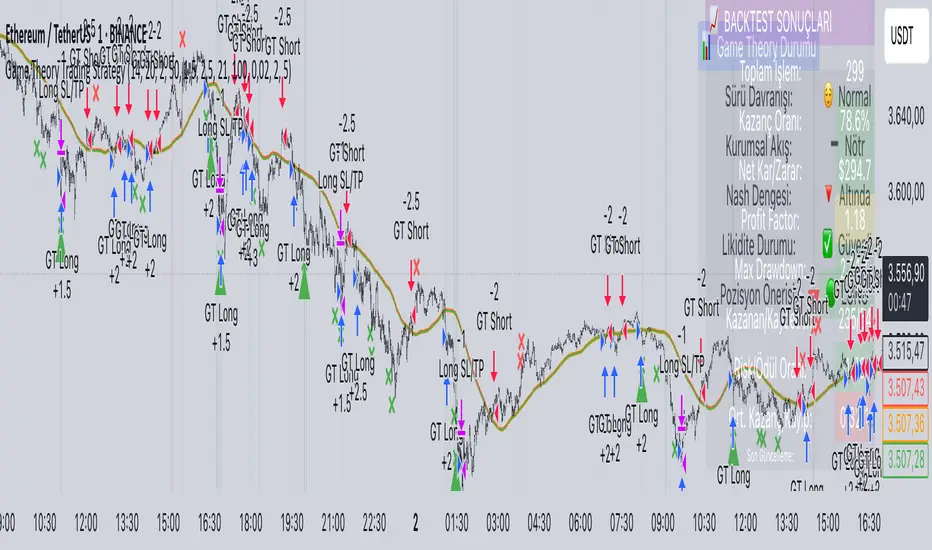
EMA9/EMA50 Cross Alert (2H Only)התראה לקרוס של ממוצע נא אקספוננציאלי 9 ו 50 ל 2 הכיוונים בטיים פרם של שעתיים.
Alert for a collapse of the 9 and 50 exponential moving averages in both directions on a two-hour time frame.
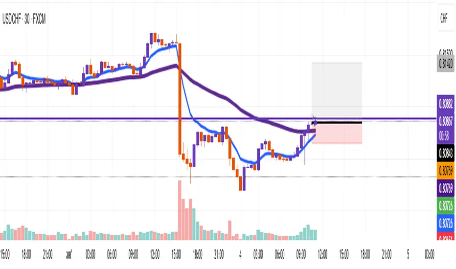
トレンドフォローBUY&SELL ver1.1Indicator Description
This indicator displays three moving averages (MAs) and generates buy and sell signals based on their crossovers. It’s designed to help traders easily follow the trend and avoid counter-trend trades.
1. Three Moving Averages
MA1 (Default: 7) – Short-term trend (Yellow)
MA2 (Default: 50) – Medium-term trend (Blue)
MA3 (Default: 200) – Long-term trend (Red), also used as a filter
2. Signal Types
(A) MA1 and MA3 Crossovers (Yellow Signals)
Golden Cross (BUY): MA1 crosses above MA3
Dead Cross (SELL): MA1 crosses below MA3
→ Helps identify shifts between short-term and long-term trends.
(B) MA1 and MA2 Crossovers (Green & Red Signals)
BUY (Green): MA1 and MA2 cross, and both are above MA3
SELL (Red): MA1 and MA2 cross, and both are below MA3
→ Only trend-aligned signals are shown (buy only above MA3, sell only below MA3).
(C) Gray Signals (Filtered-Out Signals)
If MA1 and MA2 cross but don’t meet the MA3 condition, a gray signal is displayed.
Example: “BUY” below MA3 or “SELL” above MA3 appears as gray.
→ This feature is ON by default but can be turned OFF in the settings.
3. Alerts
Alerts can be triggered for:
MA1 × MA3 Golden Cross / Dead Cross
MA1 × MA2 BUY / SELL (with MA3 filter)
This allows you to receive notifications when valid trade setups occur.
4. Key Benefits
Visualize short-, medium-, and long-term trends at the same time
Trade only in the direction of the 200MA trend using the built-in filter
Optionally view filtered-out (gray) signals for extra context
Set alerts to avoid missing trading opportunities
With this indicator, you can focus on trading with the trend—buying above the 200MA and selling below it—while staying informed of all crossover events.
このインジケーターは 3本の移動平均線(MA) と、
それらのクロスに基づいた 売買シグナル を表示するツールです。
1. 3本の移動平均線
MA1(デフォルト7):短期のトレンドを把握するための線(黄色)
MA2(デフォルト50):中期のトレンドを把握するための線(青)
MA3(デフォルト200):長期のトレンド(赤)。フィルターとしても使用
2. シグナルの種類
(A) MA1とMA3のクロス(黄色シグナル)
ゴールデンクロス(BUY):MA1がMA3を上抜け
デッドクロス(SELL):MA1がMA3を下抜け
→ 長期トレンドと短期の変化を確認するための参考シグナル
(B) MA1とMA2のクロス(緑・赤シグナル)
BUY(緑):MA1とMA2がクロスし、両方がMA3より上にある
SELL(赤):MA1とMA2がクロスし、両方がMA3より下にある
→ 200MAを基準に「上なら買い、下なら売り」のトレンド方向に沿ったシグナルだけを表示
(C) グレーシグナル(フィルター除外)
MA1とMA2がクロスしたが、MA3の条件を満たさなかった場合にグレー表示
例えば「MA3より下でBUY」「MA3より上でSELL」はグレー
→ 初期設定ではONになっていますが、オフにすることも可能
逆張りの指標や、トレンド転換のサインにもなる
3. アラート機能
MA1×MA3のゴールデンクロス/デッドクロス
MA1×MA2のBUY/SELL(MAフィルターあり)
→ これらが発生したタイミングでTradingViewのアラートを出せる
4. 使い方のポイント
短期・中期・長期のトレンドを同時に把握できる
200MAを基準にフィルターすることで「逆張りシグナル」を排除
フィルターで外れたシグナルもグレーで確認できる(任意)
アラートを設定すれば、チャンスを逃さずにエントリー可能
このインジケーターを使うことで、「200MAの上では買いのみ」「下では売りのみ」というシンプルでトレンドに沿ったトレードができるようになります。

ASK Screener by AshpreetThe ASK Indicator is a custom-built breakout and trend continuation system designed for swing traders seeking high-probability entries with strong risk-reward ratios. Built using a combination of moving averages, momentum filters, volume confirmation, and price structure, this indicator helps identify stocks poised for explosive moves.
It uses three key moving averages: the 44-period SMA (medium trend), 20-period DEMA (short-term strength, custom-coded), and 50-period WEMA (institutional trendline). Trades are only triggered when the price is above 50 WEMA, and the 20 DEMA is above the 44 SMA.
Momentum is confirmed using RSI(14) within a healthy zone of 40–60, ensuring the stock is not overbought or oversold. To focus on breakout candidates, the stock must be trading within 10% of its 52-week high, and the weekly candle range must be under 10%, signaling compression before expansion.
A valid ASK Signal occurs when these conditions are met along with a breakout above the previous day’s high and volume exceeding 1.5× the 20-day average. Once triggered, the indicator auto-plots the stop-loss (1× ATR) and two profit targets: 1:2 (TP1) and 1:4 (TP2).
Additionally, the system detects a narrow range setup, where the last 3 daily candles are inside the previous 3-day range — a powerful consolidation signal. Alerts for both ASK entries and narrow ranges are included.
This system is ideal for positional and short-term swing traders who want to combine structure, momentum, and volume in one powerful tool.
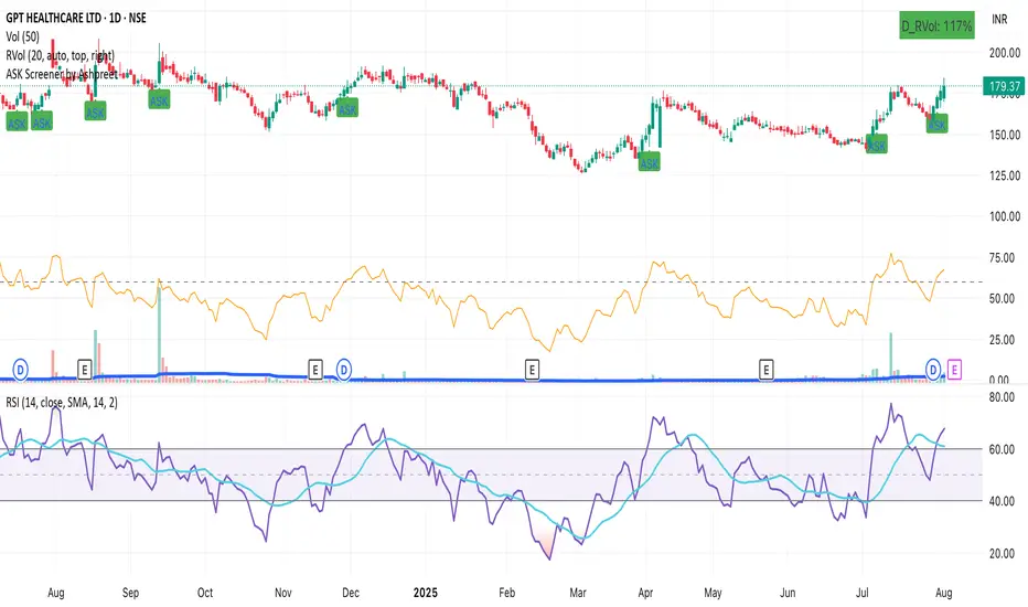
ASK Indicator by AshpreetThe ASK Indicator is a custom-built breakout and trend continuation system designed for swing traders seeking high-probability entries with strong risk-reward ratios. Built using a combination of moving averages, momentum filters, volume confirmation, and price structure, this indicator helps identify stocks poised for explosive moves.
It uses three key moving averages: the 44-period SMA (medium trend), 20-period DEMA (short-term strength, custom-coded), and 50-period WEMA (institutional trendline). Trades are only triggered when the price is above 50 WEMA, and the 20 DEMA is above the 44 SMA.
Momentum is confirmed using RSI(14) within a healthy zone of 40–60, ensuring the stock is not overbought or oversold. To focus on breakout candidates, the stock must be trading within 10% of its 52-week high, and the weekly candle range must be under 10%, signaling compression before expansion.
A valid ASK Signal occurs when these conditions are met along with a breakout above the previous day’s high and volume exceeding 1.5× the 20-day average. Once triggered, the indicator auto-plots the stop-loss (1× ATR) and two profit targets: 1:2 (TP1) and 1:4 (TP2).
Additionally, the system detects a narrow range setup, where the last 3 daily candles are inside the previous 3-day range — a powerful consolidation signal. Alerts for both ASK entries and narrow ranges are included.
This system is ideal for positional and short-term swing traders who want to combine structure, momentum, and volume in one powerful tool.
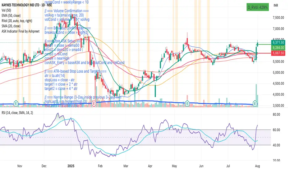
Recession Warning Model [BackQuant]Recession Warning Model
Overview
The Recession Warning Model (RWM) is a Pine Script® indicator designed to estimate the probability of an economic recession by integrating multiple macroeconomic, market sentiment, and labor market indicators. It combines over a dozen data series into a transparent, adaptive, and actionable tool for traders, portfolio managers, and researchers. The model provides customizable complexity levels, display modes, and data processing options to accommodate various analytical requirements while ensuring robustness through dynamic weighting and regime-aware adjustments.
Purpose
The RWM fulfills the need for a concise yet comprehensive tool to monitor recession risk. Unlike approaches relying on a single metric, such as yield-curve inversion, or extensive economic reports, it consolidates multiple data sources into a single probability output. The model identifies active indicators, their confidence levels, and the current economic regime, enabling users to anticipate downturns and adjust strategies accordingly.
Core Features
- Indicator Families : Incorporates 13 indicators across five categories: Yield, Labor, Sentiment, Production, and Financial Stress.
- Dynamic Weighting : Adjusts indicator weights based on recent predictive accuracy, constrained within user-defined boundaries.
- Leading and Coincident Split : Separates early-warning (leading) and confirmatory (coincident) signals, with adjustable weighting (default 60/40 mix).
- Economic Regime Sensitivity : Modulates output sensitivity based on market conditions (Expansion, Late-Cycle, Stress, Crisis), using a composite of VIX, yield-curve, financial conditions, and credit spreads.
- Display Options : Supports four modes—Probability (0-100%), Binary (four risk bins), Lead/Coincident, and Ensemble (blended probability).
- Confidence Intervals : Reflects model stability, widening during high volatility or conflicting signals.
- Alerts : Configurable thresholds (Watch, Caution, Warning, Alert) with persistence filters to minimize false signals.
- Data Export : Enables CSV output for probabilities, signals, and regimes, facilitating external analysis in Python or R.
Model Complexity Levels
Users can select from four tiers to balance simplicity and depth:
1. Essential : Focuses on three core indicators—yield-curve spread, jobless claims, and unemployment change—for minimalistic monitoring.
2. Standard : Expands to nine indicators, adding consumer confidence, PMI, VIX, S&P 500 trend, money supply vs. GDP, and the Sahm Rule.
3. Professional : Includes all 13 indicators, incorporating financial conditions, credit spreads, JOLTS vacancies, and wage growth.
4. Research : Unlocks all indicators plus experimental settings for advanced users.
Key Indicators
Below is a summary of the 13 indicators, their data sources, and economic significance:
- Yield-Curve Spread : Difference between 10-year and 3-month Treasury yields. Negative spreads signal banking sector stress.
- Jobless Claims : Four-week moving average of unemployment claims. Sustained increases indicate rising layoffs.
- Unemployment Change : Three-month change in unemployment rate. Sharp rises often precede recessions.
- Sahm Rule : Triggers when unemployment rises 0.5% above its 12-month low, a reliable recession indicator.
- Consumer Confidence : University of Michigan survey. Declines reflect household pessimism, impacting spending.
- PMI : Purchasing Managers’ Index. Values below 50 indicate manufacturing contraction.
- VIX : CBOE Volatility Index. Elevated levels suggest market anticipation of economic distress.
- S&P 500 Growth : Weekly moving average trend. Declines reduce wealth effects, curbing consumption.
- M2 + GDP Trend : Monitors money supply and real GDP. Simultaneous declines signal credit contraction.
- NFCI : Chicago Fed’s National Financial Conditions Index. Positive values indicate tighter conditions.
- Credit Spreads : Proxy for corporate bond spreads using 10-year vs. 2-year Treasury yields. Widening spreads reflect stress.
- JOLTS Vacancies : Job openings data. Significant drops precede hiring slowdowns.
- Wage Growth : Year-over-year change in average hourly earnings. Late-cycle spikes often signal economic overheating.
Data Processing
- Rate of Change (ROC) : Optionally applied to capture momentum in data series (default: 21-bar period).
- Z-Score Normalization : Standardizes indicators to a common scale (default: 252-bar lookback).
- Smoothing : Applies a short moving average to final signals (default: 5-bar period) to reduce noise.
- Binary Signals : Generated for each indicator (e.g., yield-curve inverted or PMI below 50) based on thresholds or Z-score deviations.
Probability Calculation
1. Each indicator’s binary signal is weighted according to user settings or dynamic performance.
2. Weights are normalized to sum to 100% across active indicators.
3. Leading and coincident signals are aggregated separately (if split mode is enabled) and combined using the specified mix.
4. The probability is adjusted by a regime multiplier, amplifying risk during Stress or Crisis regimes.
5. Optional smoothing ensures stable outputs.
Display and Visualization
- Probability Mode : Plots a continuous 0-100% recession probability with color gradients and confidence bands.
- Binary Mode : Categorizes risk into four levels (Minimal, Watch, Caution, Alert) for simplified dashboards.
- Lead/Coincident Mode : Displays leading and coincident probabilities separately to track signal divergence.
- Ensemble Mode : Averages traditional and split probabilities for a balanced view.
- Regime Background : Color-coded overlays (green for Expansion, orange for Late-Cycle, amber for Stress, red for Crisis).
- Analytics Table : Optional dashboard showing probability, confidence, regime, and top indicator statuses.
Practical Applications
- Asset Allocation : Adjust equity or bond exposures based on sustained probability increases.
- Risk Management : Hedge portfolios with VIX futures or options during regime shifts to Stress or Crisis.
- Sector Rotation : Shift toward defensive sectors when coincident signals rise above 50%.
- Trading Filters : Disable short-term strategies during high-risk regimes.
- Event Timing : Scale positions ahead of high-impact data releases when probability and VIX are elevated.
Configuration Guidelines
- Enable ROC and Z-score for consistent indicator comparison unless raw data is preferred.
- Use dynamic weighting with at least one economic cycle of data for optimal performance.
- Monitor stress composite scores above 80 alongside probabilities above 70 for critical risk signals.
- Adjust adaptation speed (default: 0.1) to 0.2 during Crisis regimes for faster indicator prioritization.
- Combine RWM with complementary tools (e.g., liquidity metrics) for intraday or short-term trading.
Limitations
- Macro indicators lag intraday market moves, making RWM better suited for strategic rather than tactical trading.
- Historical data availability may constrain dynamic weighting on shorter timeframes.
- Model accuracy depends on the quality and timeliness of economic data feeds.
Final Note
The Recession Warning Model provides a disciplined framework for monitoring economic downturn risks. By integrating diverse indicators with transparent weighting and regime-aware adjustments, it empowers users to make informed decisions in portfolio management, risk hedging, or macroeconomic research. Regular review of model outputs alongside market-specific tools ensures its effective application across varying market conditions.
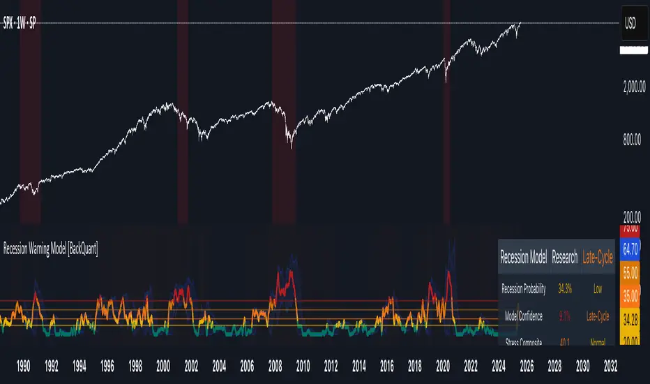
EMA Trend Confirmation with Alerts此脚本是基于EMA 200周期 50周期 20周期加以合并并进行改进的一个脚本指标,主要作用是用于观察趋势走向,其中有上升下降和震荡趋势,经过多数测试,此指标适用于短线交易,推荐周期为20或15,大周期和长线交易详见RSI+EMA结合指标
This script is an improved script indicator based on the EMA 200 period, 50 period, and 20 period. Its main function is to observe the trend direction, including up, down, and oscillating trends. After many tests, this indicator is suitable for short-term trading, and the recommended period is 20 or 15. For large-cycle and long-term trading, please refer to the RSI+EMA combination indicator.
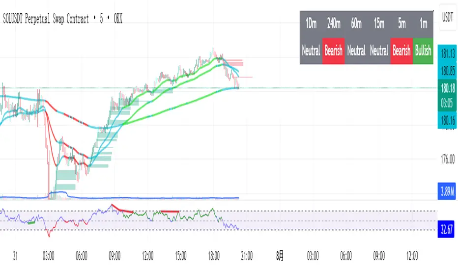
MA Crossover Detector
The Moving Average Crossover Detector is a custom indicator that visually shows buy and sell signals clearly on the chart. based on the crossing of two moving averages — a popular and beginner-friendly tool in technical analysis.
It plots two moving averages — One fast (short period) and one slow (long period) — and highlights crossover points:
✅ Buy Signal (Golden Cross) – When the fast MA crosses above the slow MA.
❌ Sell Signal (Death Cross) – When the fast MA crosses below the slow MA.
✅ Features
Visual: Clearly shows crossovers on the chart.
Customizable: Choose periods, types, styles, etc.
Alert-ready: You can set alerts for crossovers.
The Moving Average (MA) Crossover Strategy is one of the simplest and most widely used strategies in technical analysis for trading stocks, forex, crypto, and other markets. It relies on the interaction between two moving averages to generate buy and sell signals.
Core Components
Short-Term Moving Average (Fast MA) : Reacts quickly to price changes (e.g., 9-period or 20-period).
Long-Term Moving Average (Slow MA) : Reacts more slowly to price changes (e.g., 21-period or 200-period).
How the Strategy Works
Bullish Crossover (Golden Cross):
Occurs when the fast MA crosses above the slow MA. Interpreted as a buy signal, indicating a potential uptrend.
Bearish Crossover (Death Cross):
Occurs when the fast MA crosses below the slow MA. Interpreted as a sell signal, indicating a potential downtrend.
Common Variants
Short-term trading
9 EMA
21 EMA
Swing trading
20 SMA
50 SMA
Long-term investing
50 SMA
200 SMA
Pros
Easy to understand and implement
Works well in trending markets
Can be automated for backtesting and execution
Cons
Lagging indicator: MAs are based on past prices, so signals come after the move has started.
Choppy markets = whipsaws: Generates false signals in sideways/range-bound conditions.
May underperform in volatile or mean-reverting environments
Tips for Improvement
Use confirmation tools : e.g., RSI, MACD, volume analysis, price action
Add filters : Trend filter (ADX), volatility filter (ATR), or time filter (session-based)
Combine with price structure : Support/resistance, breakouts, pullbacks
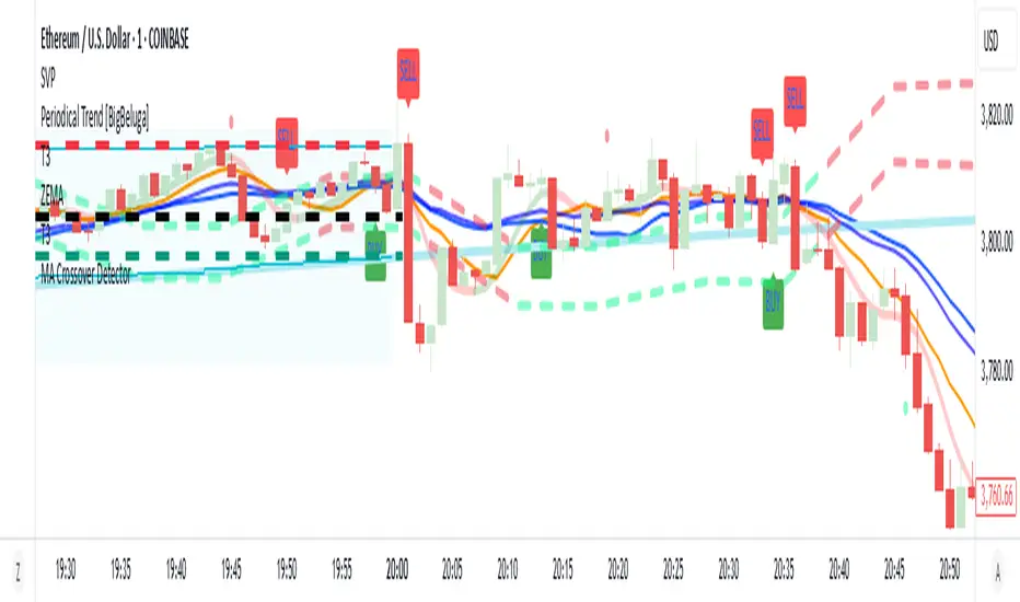
GTrader-ICT All In One-Comumnity VersionMeet the **GTrader-ICT All In One **, a comprehensive toolkit designed to integrate key Inner Circle Trader (ICT) concepts directly onto your chart. This powerful overlay indicator consolidates multiple essential tools, streamlining your technical analysis and helping you identify key temporal and price-based events.
📚 References & Inspiration
This indicator stands on the shoulders of giants. With the help of **tradeforopp** and **LuxAlgo**. The concepts and some implementation details were referenced from the following excellent, publicly available scripts:
ICT Killzones: The session drawing and pivot logic is adapted from tradeforopp
ICT Macros: The macro detection and plotting functionality is inspired by the work of Lux Algo , particularly their widely-used indicators covering ICT concepts.
🎯 Core Features
* **ICT Killzones:** Visualize critical trading sessions with customizable boxes. You can easily toggle and style the **Asia**, **London**, and **New York (AM, Lunch, PM)** sessions to focus on the liquidity and volatility that matter most to your strategy.
* Fully customizable session times and colors.
* Timezone support to align sessions with your local or preferred trading time (defaults to `America/New_York`).
* **ICT Macros:** Automatically identify and plot specific, short-duration time windows where institutional algorithms are known to be active (e.g., `09:50-10:10`, `14:50-15:10`, etc.).
* Plots the high/low range of the macro, providing clear levels of interest.
* Utilizes 1-minute data for precision, even when viewing on 3-minute or 5-minute charts.
📚 Optimization over the other original indicators
We add the custom input for macros session, users just need to input the from/to hour: minute format, and they will be converted into session objects in pinescript
The macro draws function is optimized, removing redundant draws, leading to better performance
Add "Distance from Macro Line to Chart" option
Add "Session Drawings Limit" for better performance
⚠️ Notes on TradingView Warnings
You may encounter some warnings from TradingView when using this script. These are generally expected due to the script's advanced, event-driven nature:
1. **Function Call Consistency:** The function 'box.new' should be called on each calculation for consistency, which may appear. This happens because drawing elements (like session boxes) are intentionally created only on the *first bar* of a new session, not on every single bar. This is a necessary design choice for performance and to prevent duplicate drawings.
2. **Potential for Repainting/Slow Load:** The **Macro** feature uses the `request.security_lower_tf()` function to get accurate 1-minute data. This can trigger warnings about performance or slow loading times. This is a known trade-off for achieving the precision required for the feature.

Opening-Range BreakoutNote: Default trading date range looks mediocre. Set date range to "Entire History" to see full effect of the strategy. 50.91% profitable trades, 1.178 profit factor, steady profits and limited drawdown. Total P&L: $154,141.18, Max Drawdown: $18,624.36. High R^2
█ Overview
The Opening-Range Breakout strategy is a mechanical, session‑based day‑trading system designed to capture the initial burst of directional momentum immediately following the market open. It defines a user‑configurable “opening range” window, measures its high and low boundaries, then places breakout stop orders at those levels once the range closes. Built‑in filters on minimum range width, reward‑to‑risk ratios, and optional reversal logic help refine entries and manage risk dynamically.
█ How It Works
Opening‑Range Formation
Between 9:30–10:15 AM ET (configurable), the script tracks the highest high and lowest low to form the day’s opening range box.
On the first bar after the range window closes, the range high (OR_high) and low (OR_low) are “locked in.”
Range‑Width Filter
To avoid false breakouts in low‑volatility mornings, the range must be at least X% of the current price (default 0.35%).
If the measured opening-range width < minimum threshold, no orders are placed that day.
Entry & Order Placement
Long: a stop‑buy order at the opening‑range high.
Short: a stop‑sell order at the opening‑range low.
Only one side can trigger (or both if reverse logic is enabled after a losing trade).
Risk Management
Once triggered, each trade uses an ATR‑style stop-loss defined as a percentage retracement of the range (default 50% of range width).
Profit target is set at a configurable Reward/Risk Ratio (default 1.1×).
Optional: Reverse on Stop‑Loss – if the initial breakout loses, immediately reverse into the opposite side on the same day.
Session Exit
Any open positions are closed at the end of the regular trading day (default 3:45 PM ET window end, with hard flat at session close).
Visual cues are provided via green (range high) and red (range low) step‑line plots directly on the chart, allowing you to see the range box and breakout triggers in real time.
█ Why It Works
Early Momentum Capture: The first 15 – 60 minutes of trading encapsulate overnight news digestion and institutional order flow, creating a well‑defined volatility “range.”
Mechanical Discipline: Clear, rule‑based entries and exits remove emotional guesswork, ensuring consistency.
Volatility Filtering: By requiring a minimum range width, the system avoids choppy, low‑range days where false breakouts are common.
Dynamic Sizing: Stops and targets scale with the opening range, adapting automatically to each day’s volatility environment.
█ How to Use
Set Your Instruments & Timeframe
-Apply to any futures contract on a 1‑ to 5‑minute chart.
-Ensure chart timezone is set to America/New_York.
Configure Inputs
-Opening‑Range Window: e.g. “0930-1015” for a 45‑minute range.
-Min. OR Width (%): e.g. 0.35 for 0.35% of current price.
-Reward/Risk Ratio: e.g. 1.1 for a modest profit target above your stop.
-Max OR Retracement %: e.g. 50 to set stop at 50% of range width.
-One Trade Per Day: toggle to limit to a single breakout.
-Reverse on Stop Loss: toggle to flip direction after a losing breakout.
Monitor the Chart
-Watch the green and red range boundaries form during the session open.
-Orders will automatically submit on the first bar after the range window closes, conditioned on your filters.
Review & Adjust
-Backtest across multiple months to validate performance on your preferred contract.
-Tweak range duration, minimum width, and R/R multiple to fit your risk tolerance and desired win‑rate vs. expectancy balance.
█ Settings Reference
Input Defaults
Opening‑Range Window - Time window to form OR (HHMM-HHMM) - 0930–1015
Regular Trading Day - Full session for EOD flat (HHMM-HHMM) - 0930–1545
Min. OR Width (%) - Minimum OR size as % of close to trigger orders - 0.35
Reward/Risk Ratio - Profit target multiple of stop‑loss distance - 1.1
Max OR Retracement (%) - % of OR width to use as stop‑loss distance - 50
One Trade Per Day - Limit to a single breakout order per day - false
Reverse on Stop Loss - Reverse direction immediately after a losing trade - true
Disclaimer
This strategy description and any accompanying code are provided for educational purposes only and do not constitute financial advice or a solicitation to trade. Futures trading involves substantial risk, including possible loss of capital. Past performance is not indicative of future results. Traders should assess their own risk tolerance and conduct thorough backtesting and forward-testing before committing real capital.
