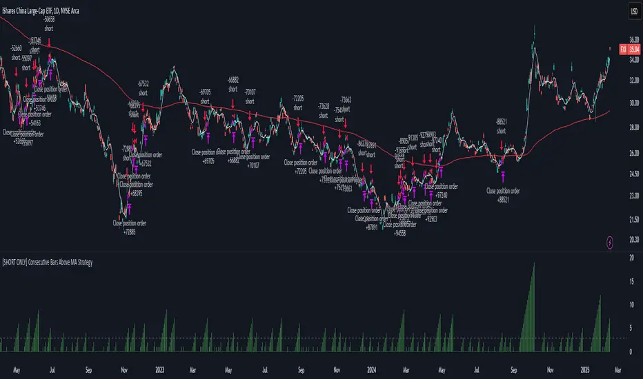
[SHORT ONLY] Consecutive Bars Above MA Strategy█ STRATEGY DESCRIPTION
The "Consecutive Bars Above MA Strategy" is a contrarian trading system aimed at exploiting overextended bullish moves in stocks and ETFs. It monitors the number of consecutive bars that close above a chosen short-term moving average (which can be either a Simple Moving Average or an Exponential Moving Average). Once the count reaches a preset threshold and the current bar’s close exceeds the previous bar’s high within a designated trading window, a short entry is initiated. An optional EMA filter further refines entries by requiring that the current close is below the 200-period EMA, helping to ensure that trades are taken in a bearish environment.
█ HOW ARE THE CONSECUTIVE BULLISH COUNTS CALCULATED?
The strategy utilizes a counter variable, `bullCount`, to track consecutive bullish bars based on their relation to the short-term moving average. Here’s how the count is determined:
Initialize the Counter
The counter is initialized at the start:
var int bullCount = na
Bullish Bar Detection
For each bar, if the close is above the selected moving average (either SMA or EMA, based on user input), the counter is incremented:
bullCount := close > signalMa ? (na(bullCount) ? 1 : bullCount + 1) : 0
Reset on Non-Bullish Condition
If the close does not exceed the moving average, the counter resets to zero, indicating a break in the consecutive bullish streak.
█ SIGNAL GENERATION
1. SHORT ENTRY
A short signal is generated when:
The number of consecutive bullish bars (i.e., bars closing above the short-term MA) meets or exceeds the defined threshold (default: 3).
The current bar’s close is higher than the previous bar’s high.
The signal occurs within the specified trading window (between Start Time and End Time).
Additionally, if the EMA filter is enabled, the entry is only executed when the current close is below the 200-period EMA.
2. EXIT CONDITION
An exit signal is triggered when the current close falls below the previous bar’s low, prompting the strategy to close the short position.
█ ADDITIONAL SETTINGS
Threshold: The number of consecutive bullish bars required to trigger a short entry (default is 3).
Trading Window: The Start Time and End Time inputs define when the strategy is active.
Moving Average Settings: Choose between SMA and EMA, and set the MA length (default is 5), which is used to assess each bar’s bullish condition.
EMA Filter (Optional): When enabled, this filter requires that the current close is below the 200-period EMA, supporting entries in a downtrend.
█ PERFORMANCE OVERVIEW
This strategy is designed for stocks and ETFs and can be applied across various timeframes.
It seeks to capture mean reversion by shorting after a series of bullish bars suggests an overextended move.
The approach employs a contrarian short entry by waiting for a breakout (close > previous high) following consecutive bullish bars.
The adjustable moving average settings and optional EMA filter allow for further optimization based on market conditions.
Comprehensive backtesting is recommended to fine-tune the threshold, moving average parameters, and filter settings for optimal performance.
Cerca negli script per "博时黄金ETF联接C基金同类基金的最大回撤率、波动率、夏普比率对比数据"
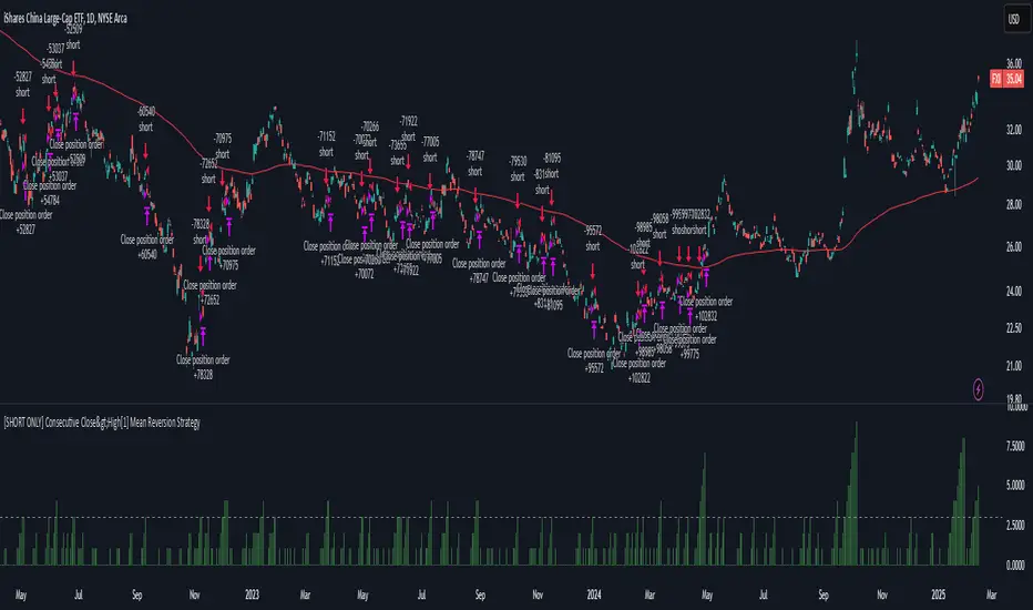
[SHORT ONLY] Consecutive Close>High[1] Mean Reversion Strategy█ STRATEGY DESCRIPTION
The "Consecutive Close > High " Mean Reversion Strategy is a contrarian daily trading system for stocks and ETFs. It identifies potential shorting opportunities by counting consecutive days where the closing price exceeds the previous day's high. When this consecutive day count reaches a predetermined threshold, and if the close is below a 200-period EMA (if enabled), a short entry is triggered, anticipating a corrective pullback.
█ HOW ARE THE CONSECUTIVE BULLISH COUNTS CALCULATED?
The strategy uses a counter variable called `bullCount` to track how many consecutive bars meet a bullish condition. Here’s a breakdown of the process:
Initialize the Counter
var int bullCount = 0
Bullish Bar Detection
Every time the close exceeds the previous bar's high, increment the counter:
if close > high
bullCount += 1
Reset on Bearish Bar
When there is a clear bearish reversal, the counter is reset to zero:
if close < low
bullCount := 0
█ SIGNAL GENERATION
1. SHORT ENTRY
A Short Signal is triggered when:
The count of consecutive bullish closes (where close > high ) reaches or exceeds the defined threshold (default: 3).
The signal occurs within the specified trading window (between Start Time and End Time).
2. EXIT CONDITION
An exit Signal is generated when the current close falls below the previous bar’s low (close < low ), prompting the strategy to exit the position.
█ ADDITIONAL SETTINGS
Threshold: The number of consecutive bullish closes required to trigger a short entry (default is 3).
Start Time and End Time: The time window during which the strategy is allowed to execute trades.
EMA Filter (Optional): When enabled, short entries are only triggered if the current close is below the 200-period EMA.
█ PERFORMANCE OVERVIEW
This strategy is designed for Stocks and ETFs on the Daily timeframe and targets overextended bullish moves.
It aims to capture mean reversion by entering short after a series of consecutive bullish closes.
Further optimization is possible with additional filters (e.g., EMA, volume, or volatility).
Backtesting should be used to fine-tune the threshold and filter settings for specific market conditions.
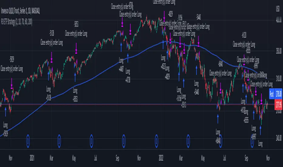
R3 ETF StrategyThis strategy is a modification of the “R3 Strategy” from the book "High Probability ETF Trading" by Larry Connors and Cesar Alvarez. This RSI strategy is for a 1-day time-frame and has these 3 simple rules:
Criteria:
The price must be above the 200 day moving average.
The 2-period (day) RSI drops 3 days in a row.
The 2-period RSI must have been below 60 3 days ago and below 10 today.
Entry and Exit:
If the 3 rules above are true, then buy on the close of the current day.
Exit on the day's close when the RSI crosses above 70.
How it works :
The Strategy will buy when the buy conditions above are true. The strategy will sell when the RSI crosses above 70. The RSI period/length, and RSI entry/exit criteria thresholds have all been coded to be adjustable with inputs.
Plots :
Blue line = 200 Day EMA (Used as Entry Criteria)
Disclaimer: Open-source scripts I publish in the community are largely meant to spark ideas that can be used as building blocks for part of a more robust trade management strategy. If you would like to implement a version of any script, I would recommend making significant additions/modifications to the strategy & risk management functions. If you don’t know how to program in Pine, then hire a Pine-coder. We can help!
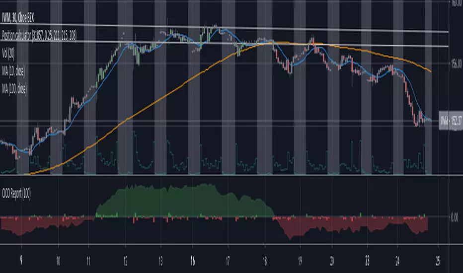
Cash in/Cash out Report (CICO) - Quiets market noiseThe cash in/cash out report (CICO for short) was built with the intent to quiet the market noise. The blunt way to say it, this indicator quiets the market manipulators voice and helps the retail investor make more money. I believe money is better of in the 99% hands versus the greedy hoarding that is currently going on. There are dozens of companies in the SP500 that have the same tax rate as unborn babies, nada. These hoarders also have machine learning high frequency trading bots that purposely create fear and anxiety in the markets. When all of the major markets move at the exact same time of day on frequent occasions, I see red flags. I recommend looking into Authorized participants in the ETF market to understand how the markets can be manipulated, specifically Creation and Redemption.
Enough of my rant. This indicator is open source. Directions on how to use the indicator can be found within the code. The basic summary is, clear your charts to bare minimums. Make the colors gray on all candles. Then apply this indicator. The indicator will color the "buy" and "sell" signals on the chart. Keep in mind, markets are manipulated to create fear in the retail investors little heart and can change drastically at any second. This indicator will show real time changes in running sum into and out of the market, it is estimated by average prices and not exact.
Once the chart is all greyed out and the indicator is applied you will see an area colored red and green. What this indicator does is takes a running sum of the new money into and out of the market. It takes the average of the high and low price times the volume. If the price is going up the value is positive, going down will be negative. Then the running sum is displayed. The area section is the running sum and the column bars are each value. When a market is steadily increasing in value you will see the large green area grow. When markets shift, values and display will change in color and vector. Full descriptions are available within the script in the comment sections.
I hope this help you make more money. If this helps you grow profits, give it a like!
Happy investing 99%er!
ETF / Stocks / Crypto - DCA Strategy v1Simple "benchmark" strategy for ETFs, Stocks and Crypto! Super-easy to implement for beginners, a DCA (dollar-cost-averaging) strategy means that you buy a fixed amount of an ETF / Stock / Crypto every several months. For instance, to DCA the S&P 500 (SPY), you could purchase $10,000 USD every 12 months, irrespective of the market price. Assuming the macro-economic conditions of the underlying country remain favourable, DCA strategies will result in capital gains over a period of many years, e.g. 10 years. DCA is the safest strategy that beginners can employ to make money in the markets, and all other types of strategies should be "benchmarked" against DCA; if your strategy cannot outperform DCA, then your strategy is useless.
Recommended Chart Settings:
Asset Class: ETF / Stocks / Crypto
Time Frame: H1 (Hourly) / D1 (Daily) / W1 (Weekly) / M1 (Monthly)
Necessary ETF Macro Conditions:
1. Country must have healthy demographics, good ratio of young > old
2. Country population must be increasing
3. Country must be experiencing price-inflation
Necessary Stock Conditions:
1. Growing revenue
2. Growing net income
3. Consistent net margins
4. Higher gross/net profit margin compared to its peers in the industry
5. Growing share holders equity
6. Current ratios > 1
7. Debt to equity ratio (compare to peers)
8. Debt servicing ratio < 30%
9. Wide economic moat
10. Products and services used daily, and will stay relevant for at least 1 decade
Necessary Crypto Conditions:
1. Honest founders
2. Competent technical co-founders
3. Fair or non-existent pre-mine
4. Solid marketing and PR
5. Legitimate use-cases / adoption
Default Robot Settings:
Contribution (USD): $10,000
Frequency (Months): 12
*Robot buys $10,000 worth of ETF, Stock, Crypto, regardless of the market price, every 12 months since its founding time.*
*Equity curve can be seen from the bottom panel*
Risk Warning:
This strategy is low-risk, however it assumes you have a long time horizon of at least 5 to 10 years. The longer your holding-period, the better your returns. The only thing the user has to keep-in-mind are the macro-economic conditions as stated above. If unsure, please stick to ETFs rather than buying individual stocks or cryptocurrencies.

BTC ETF Average Inflow Cost BasisConcept
Since the historic launch of Bitcoin Spot ETFs on January 11, 2024, institutional flows have become a major driver of price action. This indicator aims to visualize the aggregate Cost Basis (average entry price) of the major Bitcoin ETFs relative to the underlying asset.
It serves as an on-chain proxy for institutional positioning, helping traders identify critical support levels where ETF inflows have historically concentrated.
How it Works
The script aggregates daily volume data from the top Bitcoin ETFs (IBIT, FBTC, ARKB, GBTC, BITB) and compares it against the Bitcoin price (BTCUSDT).
ETF Cost Basis (Pink Line):
This is calculated as a Cumulative Volume-Weighted Average Price (VWAP), anchored specifically to the ETF launch date (Jan 11, 2024).
Formula: It accumulates (BTC Price * Total ETF Volume) and divides it by the Cumulative Total ETF Volume.
This creates a dynamic level representing the "breakeven" price for the aggregate volume traded through these funds.
True Market Mean (Gray Line):
This represents the simple cumulative average of the Bitcoin price since the ETF launch date. It acts as a neutral baseline for the post-ETF market era.
How to Use
Institutional Support: The Cost Basis line often acts as a strong dynamic support level during corrections. When price revisits this level, it suggests the market is returning to the average institutional entry price.
Trend Filter:
Price > Cost Basis: The market is in a net profit state relative to ETF flows (Bullish/Trend continuation).
Price < Cost Basis: The market is in a net loss state (Bearish/Capitulation risk).
Confluence: The intersection of the Cost Basis and the True Market Mean can signal pivotal moments of trend reset.
Features
Data Aggregation: Pulls data from 5 major ETFs via request.security without repainting (using closed bars).
Dashboard: Includes a table in the top-right corner displaying real-time values for Price, Cost Basis, and Market Mean.
Customization: You can toggle individual ETF Moving Averages in the settings (disabled by default due to price scale differences between BTC and ETF shares).
Disclaimer
This tool is for educational purposes only and attempts to estimate institutional cost basis using volume proxies. It does not represent financial advice.

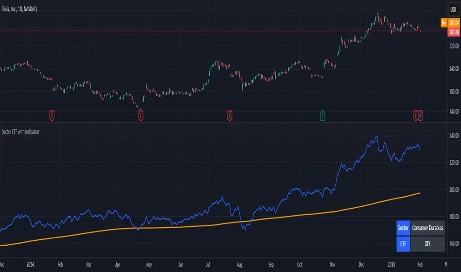
Stock ETF Tracker 2.0The Stock Sector ETF tracker with Indicators is a versatile tool designed to track the performance of sector-specific ETFs relative to the current asset. It automatically identifies the sector of the underlying symbol and displays the corresponding ETF’s price action alongside key technical indicators. This helps traders analyze sector trends and correlations in real time.
---
Key Features
Automatic Sector Detection:
Fetches the sector of the current asset (e.g., "Technology" for AAPL).
Maps the sector to a user-defined ETF (default: SPDR sector ETFs) .
Technical Indicators:
Simple Moving Average (SMA): Tracks the ETF’s trend.
Bollinger Bands: Highlights volatility and potential reversals.
Donchian High (52-Week High): Identifies long-term resistance levels.
SPY Regime Filter: Red background color if SP500 is below 200 day SMA.
Customizable Inputs:
Adjust indicator parameters (length, visibility).
Override default ETFs for specific sectors.
Informative Table:
Displays the current sector and ETF symbol in the bottom-right corner.
---
Input Settings
SMA Settings
SMA Length: Period for calculating the Simple Moving Average (default: 200).
Show SMA: Toggle visibility of the SMA line.
Bollinger Bands Settings
BB Length: Period for Bollinger Bands calculation (default: 20).
BB Multiplier: Standard deviation multiplier (default: 2.0).
Show Bollinger Bands: Toggle visibility of the bands.
Donchian High (52-Week High)
Daily High Length: Days used to calculate the high (default: 252, approx. 1 year).
Show High: Toggle visibility of the 52-week high line.
Sector Selections
Customize ETFs for each sector (e.g., replace XLU with another utilities ETF).
---
Example Use Cases
Trend Analysis: Compare a stock’s price action to its sector ETF’s SMA for trend confirmation.
Volatility Signals: Use Bollinger Bands to spot ETF price squeezes or breakouts.
Sector Strength: Monitor if the ETF is approaching its 52-week high to gauge sector momentum.
Enjoy tracking sector trends with ease! 🚀

Stock Sector ETF with IndicatorsThe Stock Sector ETF with Indicators is a versatile tool designed to track the performance of sector-specific ETFs relative to the current asset. It automatically identifies the sector of the underlying symbol and displays the corresponding ETF’s price action alongside key technical indicators. This helps traders analyze sector trends and correlations in real time.
---
Key Features
Automatic Sector Detection:
Fetches the sector of the current asset (e.g., "Technology" for AAPL).
Maps the sector to a user-defined ETF (default: SPDR sector ETFs) .
Technical Indicators:
Simple Moving Average (SMA): Tracks the ETF’s trend.
Bollinger Bands: Highlights volatility and potential reversals.
Donchian High (52-Week High): Identifies long-term resistance levels.
Customizable Inputs:
Adjust indicator parameters (length, visibility).
Override default ETFs for specific sectors.
Informative Table:
Displays the current sector and ETF symbol in the bottom-right corner.
---
Input Settings
SMA Settings
SMA Length: Period for calculating the Simple Moving Average (default: 200).
Show SMA: Toggle visibility of the SMA line.
Bollinger Bands Settings
BB Length: Period for Bollinger Bands calculation (default: 20).
BB Multiplier: Standard deviation multiplier (default: 2.0).
Show Bollinger Bands: Toggle visibility of the bands.
Donchian High (52-Week High)
Daily High Length: Days used to calculate the high (default: 252, approx. 1 year).
Show High: Toggle visibility of the 52-week high line.
Sector Selections
Customize ETFs for each sector (e.g., replace XLU with another utilities ETF).
---
Example Use Cases
Trend Analysis: Compare a stock’s price action to its sector ETF’s SMA for trend confirmation.
Volatility Signals: Use Bollinger Bands to spot ETF price squeezes or breakouts.
Sector Strength: Monitor if the ETF is approaching its 52-week high to gauge sector momentum.
Enjoy tracking sector trends with ease! 🚀
Crypto ETFs AUM📘 Description: BTC ETFs AUM Tracker
This indicator tracks the Assets Under Management (AUM) and daily inflows/outflows of the main U.S.-listed Bitcoin ETFs, allowing you to visualize institutional capital movement into Bitcoin products over time. It helps traders correlate institutional capital movement with Bitcoin price behavior.
🧩 Overview
The script adds up the daily AUM changes from selected Bitcoin ETFs to estimate the total net inflow/outflow of capital into spot BTC funds. It also accumulates those flows over time to display the total aggregated AUM balance, giving you a clearer sense of market direction and institutional sentiment. Two display modes are available: Balance view: plots the cumulative sum of net inflows (total ETF AUM). Inflows view: shows daily inflows (green) and outflows (red) as histogram columns, together with a smoothed moving average line.
⚙️ Inputs
Explained Base Settings Base Multiplier (base_multi) – Scaling factor applied to all AUM values. Leave at 1 for USD units, or adjust to display values in millions (1e6) or billions (1e9). Smoothing (c_smoothing) – Period length for the simple moving average used to calculate the smoothed mean inflow/outflow line. Show Balance (showBalance) – When enabled, displays the total cumulative AUM balance (sum of all net inflows over time). Show Inflows (showInflows) – When enabled, displays the daily inflows/outflows as colored columns. ETF Selection You can toggle which ETFs are included in the calculation:
BIT (BlackRock)
GBTC (Grayscale)
FBTC (Fidelity)
ARKB (ARK/21Shares)
BITB (Bitwise)
EZBC (Franklin Templeton)
BTCW (WisdomTree)
BTCO (Invesco Galaxy)
BRRR (Valkyrie)
HODL (VanEck)
Each switch determines whether the ETF’s AUM and daily flow data are included in the total calculation.
📊 Displayed Values Green Columns → Positive daily net inflows (AUM increased). Red Columns → Negative daily net outflows (AUM decreased). Orange Line → Smoothed moving average of net flows, used to identify persistent inflow/outflow trends. Blue Line (if enabled) → Total cumulative AUM balance (sum of all historical flows).
💡 Usage Notes Works best on daily timeframe, since ETF data is typically updated once per trading day. Not all ETFs have identical data history; missing data points are automatically skipped. The indicator doesn’t represent official fund NAV or guarantee data accuracy — it visualizes TradingView’s public financial feed. You can combine this tool with price action or on-chain metrics to analyze institutional Bitcoin flows.
Note: Some ETF data may not be available to all users depending on their TradingView data subscription or market access. Missing values are automatically skipped.
🧠 Disclaimer This script is for educational and analytical purposes only. It is not financial advice, and no investment decisions should be based solely on this indicator. Data accuracy depends on TradingView’s financial data sources and exchange reporting frequency.

[MAD] BTC ETF Volume In/OutflowThe " BTC ETF Volume In/Outflows" indicator is designed to analyze and visualize the volume data of various Bitcoin Exchange-Traded Funds (ETFs) across different exchanges. This indicator helps traders and analysts observe the inflows and outflows of trading volume in a structured and comparative manner.
Features
Multi-Ticker Support: The indicator is capable of handling volume data from multiple ETFs simultaneously, making it versatile for comparative analysis.
Volume Adjustments: Provides an option to view volume data either as the number of pieces (shares) traded or as monetary flow (value traded).
Compression Factor: Includes a volume compression factor setting that helps in emphasizing smaller volume changes or smoothing out volume spikes.
Data Calculation
Volume data is processed using a custom function that adjusts the data based on user settings for piece or monetary representation and applies a logarithmic compression factor.
This processed data is then fetched for each ticker.
Visualization
Volume data is visualized on the chart using column plots where each ETF's volume data is stacked and offset to provide a clear visual representation of in/outflows. Horizontal lines indicate the zero level for reference.
Usage Scenario
This indicator is particularly useful for traders who track multiple ETFs and need to compare their volume activities simultaneously. It provides insights into market trends, potentially indicating bullish or bearish shifts based on volume inflows and outflows across different instruments.
have fun :-)

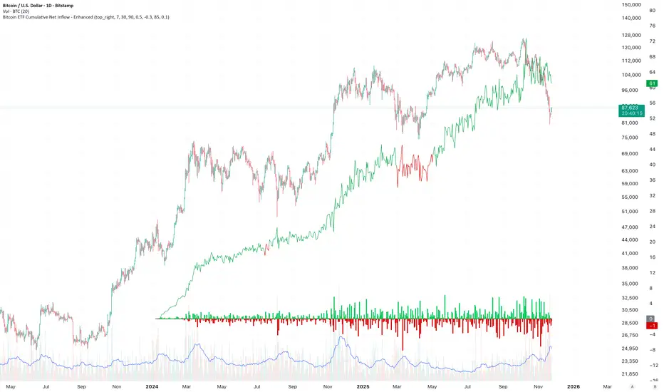
Bitcoin ETF Cumulative Net InflowIndicator Description:
This indicator calculates and plots the cumulative net inflow (in billions of USD) for selected Bitcoin ETFs on the main price chart. It uses AUM data from TradingView to estimate daily net flows, adjusted for BTC price changes, and accumulates them over time. The line is overlaid on the price chart (e.g., BTCUSD) with a right scale for better visibility, helping to identify correlations between ETF inflows and Bitcoin price movements.
Key Features:
Supports selection of 10 major Bitcoin ETFs (IBIT, FBTC, ARKB, etc.) via inputs.
Cumulative inflow line (purple, linewidth=2) for trend analysis.
Data sourced from request.financial("AUM", "D") for accuracy.
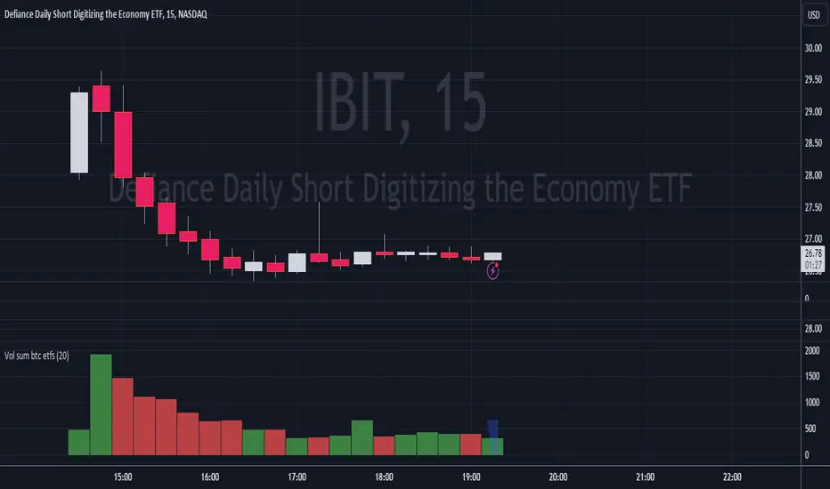
Volume Sum BTC ETFsThis volume indicator tracks the volume of these 10 bitcoin ETFS:
AMEX:GBTC, NASDAQ:IBIT, AMEX:BTCO, AMEX:ARKB, AMEX:HODL, AMEX:EZBC, NASDAQ:BRRR, AMEX:BTCW, AMEX:DEFI, AMEX:BITB
It multiplies the traded shares with the hl2 share price and then devides the volume by the bitcoin hl2 price.
You can change to usd volume in settings.
Enjoy!
Notice that historical volume comes from etfs which traded already before launch like GBTC.
Also notice that that btc trades also when tradfi markets are closed, so then the indicator will show the last available volume. Something to fix later.
Ray Dalio's All Weather Strategy - Portfolio CalculatorTHE ALL WEATHER STRATEGY INDICATOR: A GUIDE TO RAY DALIO'S LEGENDARY PORTFOLIO APPROACH
Introduction: The Genesis of Financial Resilience
In the sprawling corridors of Bridgewater Associates, the world's largest hedge fund managing over 150 billion dollars in assets, Ray Dalio conceived what would become one of the most influential investment strategies of the modern era. The All Weather Strategy, born from decades of market observation and rigorous backtesting, represents a paradigm shift from traditional portfolio construction methods that have dominated Wall Street since Harry Markowitz's seminal work on Modern Portfolio Theory in 1952.
Unlike conventional approaches that chase returns through market timing or stock picking, the All Weather Strategy embraces a fundamental truth that has humbled countless investors throughout history: nobody can consistently predict the future direction of markets. Instead of fighting this uncertainty, Dalio's approach harnesses it, creating a portfolio designed to perform reasonably well across all economic environments, hence the evocative name "All Weather."
The strategy emerged from Bridgewater's extensive research into economic cycles and asset class behavior, culminating in what Dalio describes as "the Holy Grail of investing" in his bestselling book "Principles" (Dalio, 2017). This Holy Grail isn't about achieving spectacular returns, but rather about achieving consistent, risk-adjusted returns that compound steadily over time, much like the tortoise defeating the hare in Aesop's timeless fable.
HISTORICAL DEVELOPMENT AND EVOLUTION
The All Weather Strategy's origins trace back to the tumultuous economic periods of the 1970s and 1980s, when traditional portfolio construction methods proved inadequate for navigating simultaneous inflation and recession. Raymond Thomas Dalio, born in 1949 in Queens, New York, founded Bridgewater Associates from his Manhattan apartment in 1975, initially focusing on currency and fixed-income consulting for corporate clients.
Dalio's early experiences during the 1970s stagflation period profoundly shaped his investment philosophy. Unlike many of his contemporaries who viewed inflation and deflation as opposing forces, Dalio recognized that both conditions could coexist with either economic growth or contraction, creating four distinct economic environments rather than the traditional two-factor models that dominated academic finance.
The conceptual breakthrough came in the late 1980s when Dalio began systematically analyzing asset class performance across different economic regimes. Working with a small team of researchers, Bridgewater developed sophisticated models that decomposed economic conditions into growth and inflation components, then mapped historical asset class returns against these regimes. This research revealed that traditional portfolio construction, heavily weighted toward stocks and bonds, left investors vulnerable to specific economic scenarios.
The formal All Weather Strategy emerged in 1996 when Bridgewater was approached by a wealthy family seeking a portfolio that could protect their wealth across various economic conditions without requiring active management or market timing. Unlike Bridgewater's flagship Pure Alpha fund, which relied on active trading and leverage, the All Weather approach needed to be completely passive and unleveraged while still providing adequate diversification.
Dalio and his team spent months developing and testing various allocation schemes, ultimately settling on the 30/40/15/7.5/7.5 framework that balances risk contributions rather than dollar amounts. This approach was revolutionary because it focused on risk budgeting—ensuring that no single asset class dominated the portfolio's risk profile—rather than the traditional approach of equal dollar allocations or market-cap weighting.
The strategy's first institutional implementation began in 1996 with a family office client, followed by gradual expansion to other wealthy families and eventually institutional investors. By 2005, Bridgewater was managing over $15 billion in All Weather assets, making it one of the largest systematic strategy implementations in institutional investing.
The 2008 financial crisis provided the ultimate test of the All Weather methodology. While the S&P 500 declined by 37% and many hedge funds suffered double-digit losses, the All Weather strategy generated positive returns, validating Dalio's risk-balancing approach. This performance during extreme market stress attracted significant institutional attention, leading to rapid asset growth in subsequent years.
The strategy's theoretical foundations evolved throughout the 2000s as Bridgewater's research team, led by co-chief investment officers Greg Jensen and Bob Prince, refined the economic framework and incorporated insights from behavioral economics and complexity theory. Their research, published in numerous institutional white papers, demonstrated that traditional portfolio optimization methods consistently underperformed simpler risk-balanced approaches across various time periods and market conditions.
Academic validation came through partnerships with leading business schools and collaboration with prominent economists. The strategy's risk parity principles influenced an entire generation of institutional investors, leading to the creation of numerous risk parity funds managing hundreds of billions in aggregate assets.
In recent years, the democratization of sophisticated financial tools has made All Weather-style investing accessible to individual investors through ETFs and systematic platforms. The availability of high-quality, low-cost ETFs covering each required asset class has eliminated many of the barriers that previously limited sophisticated portfolio construction to institutional investors.
The development of advanced portfolio management software and platforms like TradingView has further democratized access to institutional-quality analytics and implementation tools. The All Weather Strategy Indicator represents the culmination of this trend, providing individual investors with capabilities that previously required teams of portfolio managers and risk analysts.
Understanding the Four Economic Seasons
The All Weather Strategy's theoretical foundation rests on Dalio's observation that all economic environments can be characterized by two primary variables: economic growth and inflation. These variables create four distinct "economic seasons," each favoring different asset classes. Rising growth benefits stocks and commodities, while falling growth favors bonds. Rising inflation helps commodities and inflation-protected securities, while falling inflation benefits nominal bonds and stocks.
This framework, detailed extensively in Bridgewater's research papers from the 1990s, suggests that by holding assets that perform well in each economic season, an investor can create a portfolio that remains resilient regardless of which season unfolds. The elegance lies not in predicting which season will occur, but in being prepared for all of them simultaneously.
Academic research supports this multi-environment approach. Ang and Bekaert (2002) demonstrated that regime changes in economic conditions significantly impact asset returns, while Fama and French (2004) showed that different asset classes exhibit varying sensitivities to economic factors. The All Weather Strategy essentially operationalizes these academic insights into a practical investment framework.
The Original All Weather Allocation: Simplicity Masquerading as Sophistication
The core All Weather portfolio, as implemented by Bridgewater for institutional clients and later adapted for retail investors, maintains a deceptively simple static allocation: 30% stocks, 40% long-term bonds, 15% intermediate-term bonds, 7.5% commodities, and 7.5% Treasury Inflation-Protected Securities (TIPS). This allocation may appear arbitrary to the uninitiated, but each percentage reflects careful consideration of historical volatilities, correlations, and economic sensitivities.
The 30% stock allocation provides growth exposure while limiting the portfolio's overall volatility. Stocks historically deliver superior long-term returns but with significant volatility, as evidenced by the Standard & Poor's 500 Index's average annual return of approximately 10% since 1926, accompanied by standard deviation exceeding 15% (Ibbotson Associates, 2023). By limiting stock exposure to 30%, the portfolio captures much of the equity risk premium while avoiding excessive volatility.
The combined 55% allocation to bonds (40% long-term plus 15% intermediate-term) serves as the portfolio's stabilizing force. Long-term bonds provide substantial interest rate sensitivity, performing well during economic slowdowns when central banks reduce rates. Intermediate-term bonds offer a balance between interest rate sensitivity and reduced duration risk. This bond-heavy allocation reflects Dalio's insight that bonds typically exhibit lower volatility than stocks while providing essential diversification benefits.
The 7.5% commodities allocation addresses inflation protection, as commodity prices typically rise during inflationary periods. Historical analysis by Bodie and Rosansky (1980) demonstrated that commodities provide meaningful diversification benefits and inflation hedging capabilities, though with considerable volatility. The relatively small allocation reflects commodities' high volatility and mixed long-term returns.
Finally, the 7.5% TIPS allocation provides explicit inflation protection through government-backed securities whose principal and interest payments adjust with inflation. Introduced by the U.S. Treasury in 1997, TIPS have proven effective inflation hedges, though they underperform nominal bonds during deflationary periods (Campbell & Viceira, 2001).
Historical Performance: The Evidence Speaks
Analyzing the All Weather Strategy's historical performance reveals both its strengths and limitations. Using monthly return data from 1970 to 2023, spanning over five decades of varying economic conditions, the strategy has delivered compelling risk-adjusted returns while experiencing lower volatility than traditional stock-heavy portfolios.
During this period, the All Weather allocation generated an average annual return of approximately 8.2%, compared to 10.5% for the S&P 500 Index. However, the strategy's annual volatility measured just 9.1%, substantially lower than the S&P 500's 15.8% volatility. This translated to a Sharpe ratio of 0.67 for the All Weather Strategy versus 0.54 for the S&P 500, indicating superior risk-adjusted performance.
More impressively, the strategy's maximum drawdown over this period was 12.3%, occurring during the 2008 financial crisis, compared to the S&P 500's maximum drawdown of 50.9% during the same period. This drawdown mitigation proves crucial for long-term wealth building, as Stein and DeMuth (2003) demonstrated that avoiding large losses significantly impacts compound returns over time.
The strategy performed particularly well during periods of economic stress. During the 1970s stagflation, when stocks and bonds both struggled, the All Weather portfolio's commodity and TIPS allocations provided essential protection. Similarly, during the 2000-2002 dot-com crash and the 2008 financial crisis, the portfolio's bond-heavy allocation cushioned losses while maintaining positive returns in several years when stocks declined significantly.
However, the strategy underperformed during sustained bull markets, particularly the 1990s technology boom and the 2010s post-financial crisis recovery. This underperformance reflects the strategy's conservative nature and diversified approach, which sacrifices potential upside for downside protection. As Dalio frequently emphasizes, the All Weather Strategy prioritizes "not losing money" over "making a lot of money."
Implementing the All Weather Strategy: A Practical Guide
The All Weather Strategy Indicator transforms Dalio's institutional-grade approach into an accessible tool for individual investors. The indicator provides real-time portfolio tracking, rebalancing signals, and performance analytics, eliminating much of the complexity traditionally associated with implementing sophisticated allocation strategies.
To begin implementation, investors must first determine their investable capital. As detailed analysis reveals, the All Weather Strategy requires meaningful capital to implement effectively due to transaction costs, minimum investment requirements, and the need for precise allocations across five different asset classes.
For portfolios below $50,000, the strategy becomes challenging to implement efficiently. Transaction costs consume a disproportionate share of returns, while the inability to purchase fractional shares creates allocation drift. Consider an investor with $25,000 attempting to allocate 7.5% to commodities through the iPath Bloomberg Commodity Index ETF (DJP), currently trading around $25 per share. This allocation targets $1,875, enough for only 75 shares, creating immediate tracking error.
At $50,000, implementation becomes feasible but not optimal. The 30% stock allocation ($15,000) purchases approximately 37 shares of the SPDR S&P 500 ETF (SPY) at current prices around $400 per share. The 40% long-term bond allocation ($20,000) buys 200 shares of the iShares 20+ Year Treasury Bond ETF (TLT) at approximately $100 per share. While workable, these allocations leave significant cash drag and rebalancing challenges.
The optimal minimum for individual implementation appears to be $100,000. At this level, each allocation becomes substantial enough for precise implementation while keeping transaction costs below 0.4% annually. The $30,000 stock allocation, $40,000 long-term bond allocation, $15,000 intermediate-term bond allocation, $7,500 commodity allocation, and $7,500 TIPS allocation each provide sufficient size for effective management.
For investors with $250,000 or more, the strategy implementation approaches institutional quality. Allocation precision improves, transaction costs decline as a percentage of assets, and rebalancing becomes highly efficient. These larger portfolios can also consider adding complexity through international diversification or alternative implementations.
The indicator recommends quarterly rebalancing to balance transaction costs with allocation discipline. Monthly rebalancing increases costs without substantial benefits for most investors, while annual rebalancing allows excessive drift that can meaningfully impact performance. Quarterly rebalancing, typically on the first trading day of each quarter, provides an optimal balance.
Understanding the Indicator's Functionality
The All Weather Strategy Indicator operates as a comprehensive portfolio management system, providing multiple analytical layers that professional money managers typically reserve for institutional clients. This sophisticated tool transforms Ray Dalio's institutional-grade strategy into an accessible platform for individual investors, offering features that rival professional portfolio management software.
The indicator's core architecture consists of several interconnected modules that work seamlessly together to provide complete portfolio oversight. At its foundation lies a real-time portfolio simulation engine that tracks the exact value of each ETF position based on current market prices, eliminating the need for manual calculations or external spreadsheets.
DETAILED INDICATOR COMPONENTS AND FUNCTIONS
Portfolio Configuration Module
The portfolio setup begins with the Portfolio Configuration section, which establishes the fundamental parameters for strategy implementation. The Portfolio Capital input accepts values from $1,000 to $10,000,000, accommodating everyone from beginning investors to institutional clients. This input directly drives all subsequent calculations, determining exact share quantities and portfolio values throughout the implementation period.
The Portfolio Start Date function allows users to specify when they began implementing the All Weather Strategy, creating a clear demarcation point for performance tracking. This feature proves essential for investors who want to track their actual implementation against theoretical performance, providing realistic assessment of strategy effectiveness including timing differences and implementation costs.
Rebalancing Frequency settings offer two options: Monthly and Quarterly. While monthly rebalancing provides more precise allocation control, quarterly rebalancing typically proves more cost-effective for most investors due to reduced transaction costs. The indicator automatically detects the first trading day of each period, ensuring rebalancing occurs at optimal times regardless of weekends, holidays, or market closures.
The Rebalancing Threshold parameter, adjustable from 0.5% to 10%, determines when allocation drift triggers rebalancing recommendations. Conservative settings like 1-2% maintain tight allocation control but increase trading frequency, while wider thresholds like 3-5% reduce trading costs but allow greater allocation drift. This flexibility accommodates different risk tolerances and cost structures.
Visual Display System
The Show All Weather Calculator toggle controls the main dashboard visibility, allowing users to focus on chart visualization when detailed metrics aren't needed. When enabled, this comprehensive dashboard displays current portfolio value, individual ETF allocations, target versus actual weights, rebalancing status, and performance metrics in a professionally formatted table.
Economic Environment Display provides context about current market conditions based on growth and inflation indicators. While simplified compared to Bridgewater's sophisticated regime detection, this feature helps users understand which economic "season" currently prevails and which asset classes should theoretically benefit.
Rebalancing Signals illuminate when portfolio drift exceeds user-defined thresholds, highlighting specific ETFs that require adjustment. These signals use color coding to indicate urgency: green for balanced allocations, yellow for moderate drift, and red for significant deviations requiring immediate attention.
Advanced Label System
The rebalancing label system represents one of the indicator's most innovative features, providing three distinct detail levels to accommodate different user needs and experience levels. The "None" setting displays simple symbols marking portfolio start and rebalancing events without cluttering the chart with text. This minimal approach suits experienced investors who understand the implications of each symbol.
"Basic" label mode shows essential information including portfolio values at each rebalancing point, enabling quick assessment of strategy performance over time. These labels display "START $X" for portfolio initiation and "RBL $Y" for rebalancing events, providing clear performance tracking without overwhelming detail.
"Detailed" labels provide comprehensive trading instructions including exact buy and sell quantities for each ETF. These labels might display "RBL $125,000 BUY 15 SPY SELL 25 TLT BUY 8 IEF NO TRADES DJP SELL 12 SCHP" providing complete implementation guidance. This feature essentially transforms the indicator into a personal portfolio manager, eliminating guesswork about exact trades required.
Professional Color Themes
Eight professionally designed color themes adapt the indicator's appearance to different aesthetic preferences and market analysis styles. The "Gold" theme reflects traditional wealth management aesthetics, while "EdgeTools" provides modern professional appearance. "Behavioral" uses psychologically informed colors that reinforce disciplined decision-making, while "Quant" employs high-contrast combinations favored by quantitative analysts.
"Ocean," "Fire," "Matrix," and "Arctic" themes provide distinctive visual identities for traders who prefer unique chart aesthetics. Each theme automatically adjusts for dark or light mode optimization, ensuring optimal readability across different TradingView configurations.
Real-Time Portfolio Tracking
The portfolio simulation engine continuously tracks five separate ETF positions: SPY for stocks, TLT for long-term bonds, IEF for intermediate-term bonds, DJP for commodities, and SCHP for TIPS. Each position's value updates in real-time based on current market prices, providing instant feedback about portfolio performance and allocation drift.
Current share calculations determine exact holdings based on the most recent rebalancing, while target shares reflect optimal allocation based on current portfolio value. Trade calculations show precisely how many shares to buy or sell during rebalancing, eliminating manual calculations and potential errors.
Performance Analytics Suite
The indicator's performance measurement capabilities rival professional portfolio analysis software. Sharpe ratio calculations incorporate current risk-free rates obtained from Treasury yield data, providing accurate risk-adjusted performance assessment. Volatility measurements use rolling periods to capture changing market conditions while maintaining statistical significance.
Portfolio return calculations track both absolute and relative performance, comparing the All Weather implementation against individual asset classes and benchmark indices. These metrics update continuously, providing real-time assessment of strategy effectiveness and implementation quality.
Data Quality Monitoring
Sophisticated data quality checks ensure reliable indicator operation across different market conditions and potential data interruptions. The system monitors all five ETF price feeds plus economic data sources, providing quality scores that alert users to potential data issues that might affect calculations.
When data quality degrades, the indicator automatically switches to fallback values or alternative data sources, maintaining functionality during temporary market data interruptions. This robust design ensures consistent operation even during volatile market conditions when data feeds occasionally experience disruptions.
Risk Management and Behavioral Considerations
Despite its sophisticated design, the All Weather Strategy faces behavioral challenges that have derailed countless well-intentioned investment plans. The strategy's conservative nature means it will underperform growth stocks during bull markets, potentially by substantial margins. Maintaining discipline during these periods requires understanding that the strategy optimizes for risk-adjusted returns over absolute returns.
Behavioral finance research by Kahneman and Tversky (1979) demonstrates that investors feel losses approximately twice as intensely as equivalent gains. This loss aversion creates powerful psychological pressure to abandon defensive strategies during bull markets when aggressive portfolios appear more attractive. The All Weather Strategy's bond-heavy allocation will seem overly conservative when technology stocks double in value, as occurred repeatedly during the 2010s.
Conversely, the strategy's defensive characteristics provide psychological comfort during market stress. When stocks crash 30-50%, as they periodically do, the All Weather portfolio's modest losses feel manageable rather than catastrophic. This emotional stability enables investors to maintain their investment discipline when others capitulate, often at the worst possible times.
Rebalancing discipline presents another behavioral challenge. Selling winners to buy losers contradicts natural human tendencies but remains essential for the strategy's success. When stocks have outperformed bonds for several quarters, rebalancing requires selling high-performing stock positions to purchase seemingly stagnant bond positions. This action feels counterintuitive but captures the strategy's systematic approach to risk management.
Tax considerations add complexity for taxable accounts. Frequent rebalancing generates taxable events that can erode after-tax returns, particularly for high-income investors facing elevated capital gains rates. Tax-advantaged accounts like 401(k)s and IRAs provide ideal vehicles for All Weather implementation, eliminating tax friction from rebalancing activities.
Capital Requirements and Cost Analysis
Comprehensive cost analysis reveals the capital requirements for effective All Weather implementation. Annual expenses include management fees for each ETF, transaction costs from rebalancing, and bid-ask spreads from trading less liquid securities.
ETF expense ratios vary significantly across asset classes. The SPDR S&P 500 ETF charges 0.09% annually, while the iShares 20+ Year Treasury Bond ETF charges 0.20%. The iShares 7-10 Year Treasury Bond ETF charges 0.15%, the Schwab US TIPS ETF charges 0.05%, and the iPath Bloomberg Commodity Index ETF charges 0.75%. Weighted by the All Weather allocations, total expense ratios average approximately 0.19% annually.
Transaction costs depend heavily on broker selection and account size. Premium brokers like Interactive Brokers charge $1-2 per trade, resulting in $20-40 annually for quarterly rebalancing. Discount brokers may charge higher per-trade fees but offer commission-free ETF trading for selected funds. Zero-commission brokers eliminate explicit trading costs but often impose wider bid-ask spreads that function as hidden fees.
Bid-ask spreads represent the difference between buying and selling prices for each security. Highly liquid ETFs like SPY maintain spreads of 1-2 basis points, while less liquid commodity ETFs may exhibit spreads of 5-10 basis points. These costs accumulate through rebalancing activities, typically totaling 10-15 basis points annually.
For a $100,000 portfolio, total annual costs including expense ratios, transaction fees, and spreads typically range from 0.35% to 0.45%, or $350-450 annually. These costs decline as a percentage of assets as portfolio size increases, reaching approximately 0.25% for portfolios exceeding $250,000.
Comparing costs to potential benefits reveals the strategy's value proposition. Historical analysis suggests the All Weather approach reduces portfolio volatility by 35-40% compared to stock-heavy allocations while maintaining competitive returns. This volatility reduction provides substantial value during market stress, potentially preventing behavioral mistakes that destroy long-term wealth.
Alternative Implementations and Customizations
While the original All Weather allocation provides an excellent starting point, investors may consider modifications based on personal circumstances, market conditions, or geographic considerations. International diversification represents one potential enhancement, adding exposure to developed and emerging market bonds and equities.
Geographic customization becomes important for non-US investors. European investors might replace US Treasury bonds with German Bunds or broader European government bond indices. Currency hedging decisions add complexity but may reduce volatility for investors whose spending occurs in non-dollar currencies.
Tax-location strategies optimize after-tax returns by placing tax-inefficient assets in tax-advantaged accounts while holding tax-efficient assets in taxable accounts. TIPS and commodity ETFs generate ordinary income taxed at higher rates, making them candidates for retirement account placement. Stock ETFs generate qualified dividends and long-term capital gains taxed at lower rates, making them suitable for taxable accounts.
Some investors prefer implementing the bond allocation through individual Treasury securities rather than ETFs, eliminating management fees while gaining precise maturity control. Treasury auctions provide access to new securities without bid-ask spreads, though this approach requires more sophisticated portfolio management.
Factor-based implementations replace broad market ETFs with factor-tilted alternatives. Value-tilted stock ETFs, quality-focused bond ETFs, or momentum-based commodity indices may enhance returns while maintaining the All Weather framework's diversification benefits. However, these modifications introduce additional complexity and potential tracking error.
Conclusion: Embracing the Long Game
The All Weather Strategy represents more than an investment approach; it embodies a philosophy of financial resilience that prioritizes sustainable wealth building over speculative gains. In an investment landscape increasingly dominated by algorithmic trading, meme stocks, and cryptocurrency volatility, Dalio's methodical approach offers a refreshing alternative grounded in economic theory and historical evidence.
The strategy's greatest strength lies not in its potential for extraordinary returns, but in its capacity to deliver reasonable returns across diverse economic environments while protecting capital during market stress. This characteristic becomes increasingly valuable as investors approach or enter retirement, when portfolio preservation assumes greater importance than aggressive growth.
Implementation requires discipline, adequate capital, and realistic expectations. The strategy will underperform growth-oriented approaches during bull markets while providing superior downside protection during bear markets. Investors must embrace this trade-off consciously, understanding that the strategy optimizes for long-term wealth building rather than short-term performance.
The All Weather Strategy Indicator democratizes access to institutional-quality portfolio management, providing individual investors with tools previously available only to wealthy families and institutions. By automating allocation tracking, rebalancing signals, and performance analysis, the indicator removes much of the complexity that has historically limited sophisticated strategy implementation.
For investors seeking a systematic, evidence-based approach to long-term wealth building, the All Weather Strategy provides a compelling framework. Its emphasis on diversification, risk management, and behavioral discipline aligns with the fundamental principles that have created lasting wealth throughout financial history. While the strategy may not generate headlines or inspire cocktail party conversations, it offers something more valuable: a reliable path toward financial security across all economic seasons.
As Dalio himself notes, "The biggest mistake investors make is to believe that what happened in the recent past is likely to persist, and they design their portfolios accordingly." The All Weather Strategy's enduring appeal lies in its rejection of this recency bias, instead embracing the uncertainty of markets while positioning for success regardless of which economic season unfolds.
STEP-BY-STEP INDICATOR SETUP GUIDE
Setting up the All Weather Strategy Indicator requires careful attention to each configuration parameter to ensure optimal implementation. This comprehensive setup guide walks through every setting and explains its impact on strategy performance.
Initial Setup Process
Begin by adding the indicator to your TradingView chart. Search for "Ray Dalio's All Weather Strategy" in the indicator library and apply it to any chart. The indicator operates independently of the underlying chart symbol, drawing data directly from the five required ETFs regardless of which security appears on the chart.
Portfolio Configuration Settings
Start with the Portfolio Capital input, which drives all subsequent calculations. Enter your exact investable capital, ranging from $1,000 to $10,000,000. This input determines share quantities, trade recommendations, and performance calculations. Conservative recommendations suggest minimum capitals of $50,000 for basic implementation or $100,000 for optimal precision.
Select your Portfolio Start Date carefully, as this establishes the baseline for all performance calculations. Choose the date when you actually began implementing the All Weather Strategy, not when you first learned about it. This date should reflect when you first purchased ETFs according to the target allocation, creating realistic performance tracking.
Choose your Rebalancing Frequency based on your cost structure and precision preferences. Monthly rebalancing provides tighter allocation control but increases transaction costs. Quarterly rebalancing offers the optimal balance for most investors between allocation precision and cost control. The indicator automatically detects appropriate trading days regardless of your selection.
Set the Rebalancing Threshold based on your tolerance for allocation drift and transaction costs. Conservative investors preferring tight control should use 1-2% thresholds, while cost-conscious investors may prefer 3-5% thresholds. Lower thresholds maintain more precise allocations but trigger more frequent trading.
Display Configuration Options
Enable Show All Weather Calculator to display the comprehensive dashboard containing portfolio values, allocations, and performance metrics. This dashboard provides essential information for portfolio management and should remain enabled for most users.
Show Economic Environment displays current economic regime classification based on growth and inflation indicators. While simplified compared to Bridgewater's sophisticated models, this feature provides useful context for understanding current market conditions.
Show Rebalancing Signals highlights when portfolio allocations drift beyond your threshold settings. These signals use color coding to indicate urgency levels, helping prioritize rebalancing activities.
Advanced Label Customization
Configure Show Rebalancing Labels based on your need for chart annotations. These labels mark important portfolio events and can provide valuable historical context, though they may clutter charts during extended time periods.
Select appropriate Label Detail Levels based on your experience and information needs. "None" provides minimal symbols suitable for experienced users. "Basic" shows portfolio values at key events. "Detailed" provides complete trading instructions including exact share quantities for each ETF.
Appearance Customization
Choose Color Themes based on your aesthetic preferences and trading style. "Gold" reflects traditional wealth management appearance, while "EdgeTools" provides modern professional styling. "Behavioral" uses psychologically informed colors that reinforce disciplined decision-making.
Enable Dark Mode Optimization if using TradingView's dark theme for optimal readability and contrast. This setting automatically adjusts all colors and transparency levels for the selected theme.
Set Main Line Width based on your chart resolution and visual preferences. Higher width values provide clearer allocation lines but may overwhelm smaller charts. Most users prefer width settings of 2-3 for optimal visibility.
Troubleshooting Common Setup Issues
If the indicator displays "Data not available" messages, verify that all five ETFs (SPY, TLT, IEF, DJP, SCHP) have valid price data on your selected timeframe. The indicator requires daily data availability for all components.
When rebalancing signals seem inconsistent, check your threshold settings and ensure sufficient time has passed since the last rebalancing event. The indicator only triggers signals on designated rebalancing days (first trading day of each period) when drift exceeds threshold levels.
If labels appear at unexpected chart locations, verify that your chart displays percentage values rather than price values. The indicator forces percentage formatting and 0-40% scaling for optimal allocation visualization.
COMPREHENSIVE BIBLIOGRAPHY AND FURTHER READING
PRIMARY SOURCES AND RAY DALIO WORKS
Dalio, R. (2017). Principles: Life and work. New York: Simon & Schuster.
Dalio, R. (2018). A template for understanding big debt crises. Bridgewater Associates.
Dalio, R. (2021). Principles for dealing with the changing world order: Why nations succeed and fail. New York: Simon & Schuster.
BRIDGEWATER ASSOCIATES RESEARCH PAPERS
Jensen, G., Kertesz, A. & Prince, B. (2010). All Weather strategy: Bridgewater's approach to portfolio construction. Bridgewater Associates Research.
Prince, B. (2011). An in-depth look at the investment logic behind the All Weather strategy. Bridgewater Associates Daily Observations.
Bridgewater Associates. (2015). Risk parity in the context of larger portfolio construction. Institutional Research.
ACADEMIC RESEARCH ON RISK PARITY AND PORTFOLIO CONSTRUCTION
Ang, A. & Bekaert, G. (2002). International asset allocation with regime shifts. The Review of Financial Studies, 15(4), 1137-1187.
Bodie, Z. & Rosansky, V. I. (1980). Risk and return in commodity futures. Financial Analysts Journal, 36(3), 27-39.
Campbell, J. Y. & Viceira, L. M. (2001). Who should buy long-term bonds? American Economic Review, 91(1), 99-127.
Clarke, R., De Silva, H. & Thorley, S. (2013). Risk parity, maximum diversification, and minimum variance: An analytic perspective. Journal of Portfolio Management, 39(3), 39-53.
Fama, E. F. & French, K. R. (2004). The capital asset pricing model: Theory and evidence. Journal of Economic Perspectives, 18(3), 25-46.
BEHAVIORAL FINANCE AND IMPLEMENTATION CHALLENGES
Kahneman, D. & Tversky, A. (1979). Prospect theory: An analysis of decision under risk. Econometrica, 47(2), 263-292.
Thaler, R. H. & Sunstein, C. R. (2008). Nudge: Improving decisions about health, wealth, and happiness. New Haven: Yale University Press.
Montier, J. (2007). Behavioural investing: A practitioner's guide to applying behavioural finance. Chichester: John Wiley & Sons.
MODERN PORTFOLIO THEORY AND QUANTITATIVE METHODS
Markowitz, H. (1952). Portfolio selection. The Journal of Finance, 7(1), 77-91.
Sharpe, W. F. (1964). Capital asset prices: A theory of market equilibrium under conditions of risk. The Journal of Finance, 19(3), 425-442.
Black, F. & Litterman, R. (1992). Global portfolio optimization. Financial Analysts Journal, 48(5), 28-43.
PRACTICAL IMPLEMENTATION AND ETF ANALYSIS
Gastineau, G. L. (2010). The exchange-traded funds manual. 2nd ed. Hoboken: John Wiley & Sons.
Poterba, J. M. & Shoven, J. B. (2002). Exchange-traded funds: A new investment option for taxable investors. American Economic Review, 92(2), 422-427.
Israelsen, C. L. (2005). A refinement to the Sharpe ratio and information ratio. Journal of Asset Management, 5(6), 423-427.
ECONOMIC CYCLE ANALYSIS AND ASSET CLASS RESEARCH
Ilmanen, A. (2011). Expected returns: An investor's guide to harvesting market rewards. Chichester: John Wiley & Sons.
Swensen, D. F. (2009). Pioneering portfolio management: An unconventional approach to institutional investment. Rev. ed. New York: Free Press.
Siegel, J. J. (2014). Stocks for the long run: The definitive guide to financial market returns & long-term investment strategies. 5th ed. New York: McGraw-Hill Education.
RISK MANAGEMENT AND ALTERNATIVE STRATEGIES
Taleb, N. N. (2007). The black swan: The impact of the highly improbable. New York: Random House.
Lowenstein, R. (2000). When genius failed: The rise and fall of Long-Term Capital Management. New York: Random House.
Stein, D. M. & DeMuth, P. (2003). Systematic withdrawal from retirement portfolios: The impact of asset allocation decisions on portfolio longevity. AAII Journal, 25(7), 8-12.
CONTEMPORARY DEVELOPMENTS AND FUTURE DIRECTIONS
Asness, C. S., Frazzini, A. & Pedersen, L. H. (2012). Leverage aversion and risk parity. Financial Analysts Journal, 68(1), 47-59.
Roncalli, T. (2013). Introduction to risk parity and budgeting. Boca Raton: CRC Press.
Ibbotson Associates. (2023). Stocks, bonds, bills, and inflation 2023 yearbook. Chicago: Morningstar.
PERIODICALS AND ONGOING RESEARCH
Journal of Portfolio Management - Quarterly publication featuring cutting-edge research on portfolio construction and risk management
Financial Analysts Journal - Bi-monthly publication of the CFA Institute with practical investment research
Bridgewater Associates Daily Observations - Regular market commentary and research from the creators of the All Weather Strategy
RECOMMENDED READING SEQUENCE
For investors new to the All Weather Strategy, begin with Dalio's "Principles" for philosophical foundation, then proceed to the Bridgewater research papers for technical details. Supplement with Markowitz's original portfolio theory work and behavioral finance literature from Kahneman and Tversky.
Intermediate students should focus on academic papers by Ang & Bekaert on regime shifts, Clarke et al. on risk parity methods, and Ilmanen's comprehensive analysis of expected returns across asset classes.
Advanced practitioners will benefit from Roncalli's technical treatment of risk parity mathematics, Asness et al.'s academic critique of leverage aversion, and ongoing research in the Journal of Portfolio Management.

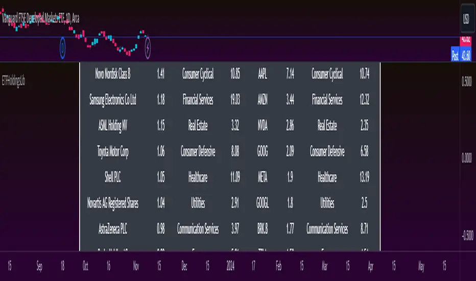
ETFHoldingsLibLibrary "ETFHoldingsLib"
spy_get()
: pulls SPY ETF data
Returns: : tickers held (string array), percent ticker holding (float array), sectors (string array), percent secture positioning (float array)
qqq_get()
: pulls QQQ ETF data
Returns: : tickers held (string array), percent ticker holding (float array), sectors (string array), percent secture positioning (float array)
arkk_get()
: pulls ARKK ETF data
Returns: : tickers held (string array), percent ticker holding (float array), sectors (string array), percent secture positioning (float array)
xle_get()
: pulls XLE ETF data
Returns: : tickers held (string array), percent ticker holding (float array), sectors (string array), percent secture positioning (float array)
brk_get()
: pulls BRK ETF data
Returns: : tickers held (string array), percent ticker holding (float array), sectors (string array), percent secture positioning (float array)
ita_get()
: pulls ITA ETF data
Returns: : tickers held (string array), percent ticker holding (float array), sectors (string array), percent secture positioning (float array)
iwm_get()
: pulls IWM ETF data
Returns: : tickers held (string array), percent ticker holding (float array), sectors (string array), percent secture positioning (float array)
xlf_get()
: pulls XLF ETF data
Returns: : tickers held (string array), percent ticker holding (float array), sectors (string array), percent secture positioning (float array)
xlv_get()
: pulls XLV ETF data
Returns: : tickers held (string array), percent ticker holding (float array), sectors (string array), percent secture positioning (float array)
vnq_get()
: pulls VNQ ETF data
Returns: : tickers held (string array), percent ticker holding (float array), sectors (string array), percent secture positioning (float array)
xbi_get()
: pulls XBI ETF data
Returns: : tickers held (string array), percent ticker holding (float array), sectors (string array), percent secture positioning (float array)
blcr_get()
: pulls BLCR ETF data
Returns: : tickers held (string array), percent ticker holding (float array), sectors (string array), percent secture positioning (float array)
vgt_get()
: pulls VGT ETF data
Returns: : tickers held (string array), percent ticker holding (float array), sectors (string array), percent secture positioning (float array)
vwo_get()
: pulls VWO ETF data
Returns: : tickers held (string array), percent ticker holding (float array), sectors (string array), percent secture positioning (float array)
vig_get()
: pulls VIG ETF data
Returns: : tickers held (string array), percent ticker holding (float array), sectors (string array), percent secture positioning (float array)
vug_get()
: pulls VUG ETF data
Returns: : tickers held (string array), percent ticker holding (float array), sectors (string array), percent secture positioning (float array)
vtv_get()
: pulls VTV ETF data
Returns: : tickers held (string array), percent ticker holding (float array), sectors (string array), percent secture positioning (float array)
vea_get()
: pulls VEA ETF data
Returns: : tickers held (string array), percent ticker holding (float array), sectors (string array), percent secture positioning (float array)
Monthly Purchase Strategy with Dynamic Contract Size This trading strategy is designed to automate monthly purchases of a security, adjusting the size of each purchase based on the percentage of the portfolio's equity. The key features of this strategy include:
Monthly Purchases: The strategy buys the security on a specified day of each month, based on the user's input.
Dynamic Position Sizing: The size of each purchase is calculated as a percentage of the current equity. This allows the position size to adjust dynamically with the portfolio's performance.
Slippage and Commission Considerations: Slippage is simulated by adjusting the entry price by a set number of ticks, while commissions are factored in as fixed costs per trade.
Drawdown Calculation: The strategy tracks the highest equity value and calculates the drawdown, which is the percentage decrease from this peak equity. This helps in assessing the performance and risk of the strategy.
Benefits of the Strategy
Automated Investment: The strategy automates the investment process, reducing the need for manual trading decisions and ensuring consistent execution.
Dynamic Position Sizing: By adjusting the purchase size based on the portfolio’s equity, the strategy helps in managing risk and capitalizing on market movements proportionally to the portfolio’s performance.
Regular Investments: Investing on a regular schedule helps in averaging the purchase price of the security, which can reduce the impact of short-term volatility.
Risk Management: Monitoring drawdown helps in assessing the risk and performance of the strategy, providing insights into potential losses relative to the highest equity value.
Scientific Documentation on ETF Savings Plans
1. Dollar-Cost Averaging and Investment Behavior:
Title: "The Benefits of Dollar-Cost Averaging: A Study of Investment Behavior"
Authors: William F. Sharpe
Journal: Financial Analysts Journal, 1994
Summary: This study discusses the concept of dollar-cost averaging (DCA), which involves investing a fixed amount of money at regular intervals regardless of market conditions. The study highlights that DCA can reduce the impact of market volatility and lower the average cost of investments over time.
Reference: Sharpe, W. F. (1994). The Benefits of Dollar-Cost Averaging: A Study of Investment Behavior. Financial Analysts Journal, 50(4), 27-36.
2. ETFs and Long-Term Investment Strategies:
Title: "Exchange-Traded Funds and Their Role in Long-Term Investment Strategies"
Authors: John C. Bogle
Journal: The Journal of Portfolio Management, 2007
Summary: This paper explores the advantages of using ETFs for long-term investment strategies, emphasizing their low costs, tax efficiency, and diversification benefits. It also discusses how ETFs can be used effectively in automated investment plans like ETF savings plans.
Reference: Bogle, J. C. (2007). Exchange-Traded Funds and Their Role in Long-Term Investment Strategies. The Journal of Portfolio Management, 33(4), 14-25.
3. Risk and Return in ETF Investments:
Title: "Risk and Return Characteristics of Exchange-Traded Funds"
Authors: Eugene F. Fama and Kenneth R. French
Journal: Journal of Financial Economics, 2010
Summary: Fama and French analyze the risk and return characteristics of ETFs compared to traditional mutual funds. The study provides insights into how ETFs can be a viable option for investors seeking diversified exposure while managing risk and optimizing returns.
Reference: Fama, E. F., & French, K. R. (2010). Risk and Return Characteristics of Exchange-Traded Funds. Journal of Financial Economics, 96(2), 257-278.
4. The Impact of Automated Investment Plans:
Title: "The Impact of Automated Investment Plans on Portfolio Performance"
Authors: David G. Blanchflower and Andrew J. Oswald
Journal: Journal of Behavioral Finance, 2012
Summary: This research examines how automated investment plans, including ETF savings plans, affect portfolio performance. It highlights the benefits of automation in reducing behavioral biases and ensuring consistent investment practices.
Reference: Blanchflower, D. G., & Oswald, A. J. (2012). The Impact of Automated Investment Plans on Portfolio Performance. Journal of Behavioral Finance, 13(2), 77-89.
Summary
The "Monthly Purchase Strategy with Dynamic Contract Size and Drawdown" provides a disciplined approach to investing by automating purchases and adjusting position sizes based on portfolio equity. It leverages the benefits of dollar-cost averaging and regular investment, with risk management through drawdown monitoring. Scientific literature supports the effectiveness of ETF savings plans and automated investment strategies in optimizing returns and managing investment risk.

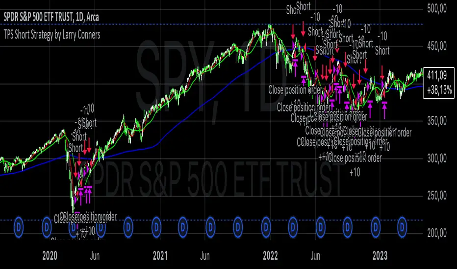
TPS Short Strategy by Larry ConnersThe TPS Short strategy aims to capitalize on extreme overbought conditions in an ETF by employing a scaling-in approach when certain technical indicators signal potential reversals. The strategy is designed to short the ETF when it is deemed overextended, based on the Relative Strength Index (RSI) and moving averages.
Components:
200-Day Simple Moving Average (SMA):
Purpose: Acts as a long-term trend filter. The ETF must be below its 200-day SMA to be eligible for shorting.
Rationale: The 200-day SMA is widely used to gauge the long-term trend of a security. When the price is below this moving average, it is often considered to be in a downtrend (Tushar S. Chande & Stanley Kroll, "The New Technical Trader: Boost Your Profit by Plugging Into the Latest Indicators").
2-Period RSI:
Purpose: Measures the speed and change of price movements to identify overbought conditions.
Criteria: Short 10% of the position when the 2-period RSI is above 75 for two consecutive days.
Rationale: A high RSI value (above 75) indicates that the ETF may be overbought, which could precede a price reversal (J. Welles Wilder, "New Concepts in Technical Trading Systems").
Scaling-In Mechanism:
Purpose: Gradually increase the short position as the ETF price rises beyond previous entry points.
Scaling Strategy:
20% more when the price is higher than the first entry.
30% more when the price is higher than the second entry.
40% more when the price is higher than the third entry.
Rationale: This incremental approach allows for an increased position size in a worsening trend, potentially increasing profitability if the trend continues to align with the strategy’s premise (Marty Schwartz, "Pit Bull: Lessons from Wall Street's Champion Day Trader").
Exit Conditions:
Criteria: Close all positions when the 2-period RSI drops below 30 or the 10-day SMA crosses above the 30-day SMA.
Rationale: A low RSI value (below 30) suggests that the ETF may be oversold and could be poised for a rebound, while the SMA crossover indicates a potential change in the trend (Martin J. Pring, "Technical Analysis Explained").
Risks and Considerations:
Market Risk:
The strategy assumes that the ETF will continue to decline once shorted. However, markets can be unpredictable, and price movements might not align with the strategy's expectations, especially in a volatile market (Nassim Nicholas Taleb, "The Black Swan: The Impact of the Highly Improbable").
Scaling Risks:
Scaling into a position as the price increases may increase exposure to adverse price movements. This method can amplify losses if the market moves against the position significantly before any reversal occurs.
Liquidity Risk:
Depending on the ETF’s liquidity, executing large trades in increments might affect the price and increase trading costs. It is crucial to ensure that the ETF has sufficient liquidity to handle large trades without significant slippage (James Altucher, "Trade Like a Hedge Fund").
Execution Risk:
The strategy relies on timely execution of trades based on specific conditions. Delays or errors in order execution can impact performance, especially in fast-moving markets.
Technical Indicator Limitations:
Technical indicators like RSI and SMA are based on historical data and may not always predict future price movements accurately. They can sometimes produce false signals, leading to potential losses if used in isolation (John Murphy, "Technical Analysis of the Financial Markets").
Conclusion
The TPS Short strategy utilizes a combination of long-term trend filtering, overbought conditions, and incremental shorting to potentially profit from price reversals. While the strategy has a structured approach and leverages well-known technical indicators, it is essential to be aware of the inherent risks, including market volatility, liquidity issues, and potential limitations of technical indicators. As with any trading strategy, thorough backtesting and risk management are crucial to its successful implementation.
TASC 2023.12 Growth and Value Switching System█ OVERVIEW
This script implements a rotation system for trading value and growth ETFs, as developed by Markos Katsanos and detailed in the article titled 'Growth Or Value?' in TASC's December 2023 edition of Traders' Tips . The purpose of this script is to demonstrate how short-term momentum can be employed to track market trends and provide clarity on when to switch between value and growth.
█ CONCEPTS
The central concept of the presented rotation strategy is based on the observation that the stock market undergoes cycles favoring either growth or value stocks. Consequently, the script introduces a momentum trading system that is designed to switch between value and growth equities based on prevailing market conditions. Specifically tailored for long-term index investors, the system focuses on trading Vanguard's value and growth ETFs ( VTV and VUG ) on a weekly timeframe.
To identify the ETF likely to outperform, the script uses a custom relative strength indicator applied to both VTV and VUG in comparison with an index ( SPY ). To minimize risk and drawdowns during bear markets, when both value and growth experience downtrends, the script employs the author's custom volume flow indicator (VFI) and blocks trades when its reading indicates money outflow . Positions are closed if the relative strength of the current open trade ETF falls below that of the other ETF for two consecutive weeks and is also below its moving average. Additionally, the script implements a stop-loss when the ETF is trading below its 40-week moving average, but only during bear markets.
The script plots the relative strengths of the value and growth equities along with the signals triggered by the aforementioned rules. Information about the current readings of the relative strength and volume flow indicators, along with the current open position, is displayed in a table.
█ CALCULATIONS
The script uses the request.security() function to gather price data for both equities and the reference index. Custom relative strength and volume flow indicators are calculated based on the formulas presented in the original article. By default, the script employs the same parameters for these indicators as proposed in the original article for VTV and VUG on a weekly timeframe.

Sector Rotation & Money Flow Dashboard📊 Overview
The Sector Rotation & Money Flow Dashboard is a comprehensive market analysis tool that tracks 39 major sector ETFs in real-time, providing institutional-grade insights into sector rotation, momentum shifts, and money flow patterns. This indicator helps traders identify which sectors are attracting capital, which are losing favor, and where the next opportunities might emerge.
Perfect for swing traders, position traders, and investors who want to stay ahead of sector rotation and ride the strongest trends while avoiding weak sectors.
🎯 What This Indicator Does
Tracks 39 Major Sectors: From technology to utilities, cryptocurrencies to commodities
Calculates Multiple Timeframes: 1-week, 1-month, 3-month, and 6-month performance
Advanced Momentum Metrics: Proprietary momentum score and acceleration calculations
Relative Strength Analysis: Compare sector performance against any benchmark index
Money Flow Signals: Visual indicators showing where institutional money is moving
Smart Filtering: Pre-built strategy filters for different trading styles
Trend Detection: Emoji-based visual system for quick trend identification
💡 Key Features
1. Performance Metrics
Multiple timeframe analysis (1W, 1M, 3M, 6M)
Month-over-month change tracking
Relative strength vs benchmark index
2. Advanced Analytics
Momentum Score: Weighted composite of recent performance
Acceleration: Rate of change in momentum (second derivative)
Money Flow Signals: IN/OUT/TURN/WATCH indicators
3. Strategy Preset Filters
🎯 Swing Trade: High momentum opportunities
📈 Trend Follow: Established uptrends
🔄 Mean Reversion: Oversold bounce candidates
💎 Value Hunt: Deep value opportunities
🚀 Breakout: Emerging strength
⚠️ Risk Off: Sectors to avoid
4. Customization
All 39 sector ETFs can be customized
Adjustable benchmark index
Flexible display options
Multiple sorting methods
📋 Settings Documentation
Display Settings
Show Table (Default: On)
Toggles the entire dashboard display
Table Position (Default: Middle Center)
Choose from 9 positions on your chart
Options: Top/Middle/Bottom × Left/Center/Right
Rows to Show (Default: 15)
Number of sectors displayed (5-40)
Useful for focusing on top/bottom performers
Sort By (Default: Momentum)
1M/3M/6M: Sort by specific timeframe performance
Momentum: Weighted recent performance score
Acceleration: Rate of momentum change
1M Change: Month-over-month improvement
RS: Relative strength vs benchmark
Flow: IN First: Prioritize sectors with inflows
Flow: TURN First: Focus on reversal candidates
Recovery Plays: Oversold sectors recovering
Oversold Bounce: Deepest declines with positive signs
Top Gainers/Losers 3M: Best/worst quarterly performers
Best Acc + Mom: Combined strength score
Worst Acc (Topping): Sectors losing momentum
Filter Settings
Strategy Preset Filter (Default: All)
All: No filtering
🎯 Swing Trade: Mom >5, Acc >2, Money flowing in
📈 Trend Follow: Positive 1M & 3M, RS >0
🔄 Mean Reversion: Oversold but improving
💎 Value Hunt: Down >10% with recovery signs
🚀 Breakout: Rapid momentum surge
⚠️ Risk Off: Declining or topping sectors
Custom Flow Filter: Use manual flow filter
Custom Flow Signal Filter (Default: All)
Only active when Strategy Preset = "Custom Flow Filter"
IN Only: Strong inflows
TURN Only: Reversal signals
WATCH Only: Recovery candidates
OUT Only: Outflow sectors
Active Flows Only: Any non-neutral signal
Hide Low Volume ETFs (Default: Off)
Filters out illiquid sectors (future enhancement)
Visual Settings
Show Trend Emojis (Default: On)
🚀 Breakout (Strong 1M + High Acceleration)
🔥 Hot Recovery (From -10% to positive)
💪 Steady Uptrend (All timeframes positive)
➡️ Sideways/Ranging
⚠️ Warning/Topping (Up >15%, now slowing)
📉 Falling (Negative + declining)
🔄 Bottoming (Improving from lows)
Compact Mode (Default: Off)
Removes decimals for cleaner display
Useful when showing many rows
Min Data Points Required (Default: 3)
Minimum data points needed to display a sector
Prevents showing sectors with insufficient data
Relative Strength Settings
RS Benchmark Index (Default: AMEX:SPY)
Index to compare all sectors against
Can use SPY, QQQ, IWM, or any other index
RS Period (Days) (Default: 21)
Lookback period for RS calculation
21 days = 1 month, 63 days = 3 months, etc.
Sector ETF Settings (Groups 1-39)
Each sector has two inputs:
Symbol: The ticker (e.g., "AMEX:XLF")
Name: Display name (e.g., "Financials")
All 39 sectors can be customized to track different ETFs or markets.
📈 Column Explanations
Sector: ETF name/description
1M%: 1-month (21-day) performance
3M%: 3-month (63-day) performance
6M%: 6-month (126-day) performance
Mom: Momentum score (weighted average, recent-biased)
Acc: Acceleration (momentum rate of change)
Δ1M: Month-over-month change
RS: Relative strength vs benchmark
Flow: Money flow signal
↗️ IN: Strong inflows
🔄 TURN: Potential reversal
👀 WATCH: Recovery candidate
↘️ OUT: Outflows
—: Neutral
🎮 Usage Tips
For Swing Traders (3-14 days)
Use "🎯 Swing Trade" filter
Sort by "Acceleration" or "Momentum"
Look for Flow = "IN" and Mom >10
Confirm with positive RS
For Position Traders (2-8 weeks)
Use "📈 Trend Follow" filter
Sort by "RS" or "Best Acc + Mom"
Focus on consistent green across timeframes
Ensure RS >3 for market leaders
For Value Investors
Use "💎 Value Hunt" filter
Sort by "Recovery Plays" or "Top Losers 3M"
Look for improving Δ1M
Check for "WATCH" or "TURN" signals
For Risk Management
Regularly check "⚠️ Risk Off" filter
Sort by "Worst Acc (Topping)"
Review holdings for ⚠️ warning emojis
Exit sectors showing "OUT" flow
Market Regime Recognition
Bull Market: Many sectors showing "IN" flow, positive RS
Bear Market: Widespread "OUT" flows, negative RS
Rotation: Mixed flows, some "IN" while others "OUT"
Recovery: Multiple "TURN" and "WATCH" signals
🔧 Pro Tips
Combine Filters + Sorting: Filter first to narrow candidates, then sort to prioritize
Multi-Timeframe Confirmation: Best setups show alignment across 1M, 3M, and momentum
RS is Key: Sectors outperforming SPY (RS >0) tend to continue outperforming
Acceleration Matters: Positive acceleration often precedes price breakouts
Flow Transitions: "WATCH" → "TURN" → "IN" progression identifies new trends early
Regular Scans:
Daily: Check "Acceleration" sort
Weekly: Review "1M Change"
Monthly: Analyze "RS" shifts
Divergence Signals:
Price up but Acceleration down = Potential top
Price down but Acceleration up = Potential bottom
Sector Pairs Trading: Long sectors with "IN" flow, short sectors with "OUT" flow
⚠️ Important Notes
This indicator makes 40 security requests (maximum allowed)
Best used on Daily timeframe
Data updates in real-time during market hours
Some ETFs may show "—" if data is unavailable
🎯 Common Strategies
"Follow the Flow"
Only trade sectors showing "IN" flow with positive RS
"Rotation Catcher"
Focus on "TURN" signals in sectors down >15% from highs
"Momentum Rider"
Trade top 3 sectors by Momentum score, exit when Acceleration turns negative
"Mean Reversion"
Buy sectors in bottom 20% by 3M performance when Δ1M improves
"Relative Strength Leader"
Maintain positions only in sectors with RS >5
Not financial advice - always do additional research

MSTY-WNTR Rebalancing SignalMSTY-WNTR Rebalancing Signal
## Overview
The **MSTY-WNTR Rebalancing Signal** is a custom TradingView indicator designed to help investors dynamically allocate between two YieldMax ETFs: **MSTY** (YieldMax MSTR Option Income Strategy ETF) and **WNTR** (YieldMax Short MSTR Option Income Strategy ETF). These ETFs are tied to MicroStrategy (MSTR) stock, which is heavily influenced by Bitcoin's price due to MSTR's significant Bitcoin holdings.
MSTY benefits from upward movements in MSTR (and thus Bitcoin) through a covered call strategy that generates income but caps upside potential. WNTR, on the other hand, provides inverse exposure, profiting from MSTR declines but losing in rallies. This indicator uses Bitcoin's momentum and MSTR's relative strength to signal when to hold MSTY (bullish phases), WNTR (bearish phases), or stay neutral, aiming to optimize returns by switching allocations at key turning points.
Inspired by strategies discussed in crypto communities (e.g., X posts analyzing MSTR-linked ETFs), this indicator promotes an active rebalancing approach over a "set and forget" buy-and-hold strategy. In simulated backtests over the past 12 months (as of August 4, 2025), the optimized version has shown potential to outperform holding 100% MSTY or 100% WNTR alone, with an illustrative APY of ~125% vs. ~6% for MSTY and ~-15% for WNTR in one scenario.
**Important Disclaimer**: This is not financial advice. Past performance does not guarantee future results. Always consult a financial advisor. Trading involves risk, and you could lose money. The indicator is for educational and informational purposes only.
## Key Features
- **Momentum-Based Signals**: Uses a Simple Moving Average (SMA) on Bitcoin's price to detect bullish (price > SMA) or bearish (price < SMA) trends.
- **RSI Confirmation**: Incorporates MSTR's Relative Strength Index (RSI) to filter signals, avoiding overbought conditions for MSTY and oversold for WNTR.
- **Visual Cues**:
- Green upward triangle for "Hold MSTY".
- Red downward triangle for "Hold WNTR".
- Yellow cross for "Switch" signals.
- Background color: Green for MSTY, red for WNTR.
- **Information Panel**: A table in the top-right corner displays real-time data: BTC Price, SMA value, MSTR RSI, and current Allocation (MSTY, WNTR, or Neutral).
- **Alerts**: Configurable alerts for holding MSTY, holding WNTR, or switching.
- **Optimized Parameters**: Defaults are tuned (SMA: 10 days, RSI: 15 periods, Overbought: 80, Oversold: 20) based on simulations to reduce whipsaws and capture trends effectively.
## How It Works
The indicator's logic is straightforward yet effective for volatile assets like Bitcoin and MSTR:
1. **Primary Trigger (Bitcoin Momentum)**:
- Calculate the SMA of Bitcoin's closing price (default: 10-day).
- Bullish: Current BTC price > SMA → Potential MSTY hold.
- Bearish: Current BTC price < SMA → Potential WNTR hold.
2. **Secondary Filter (MSTR RSI Confirmation)**:
- Compute RSI on MSTR stock (default: 15-period).
- For bullish signals: If RSI > Overbought (80), signal Neutral (avoid overextended rallies).
- For bearish signals: If RSI < Oversold (20), signal Neutral (avoid capitulation bottoms).
3. **Allocation Rules**:
- Hold 100% MSTY if bullish and not overbought.
- Hold 100% WNTR if bearish and not oversold.
- Neutral otherwise (e.g., during choppy or extreme markets) – consider holding cash or avoiding trades.
4. **Rebalancing**:
- Switch signals trigger when the hold changes (e.g., from MSTY to WNTR).
- Recommended frequency: Weekly reviews or on 5% BTC moves to minimize trading costs (aim for 4-6 trades/year).
This approach leverages Bitcoin's influence on MSTR while mitigating the risks of MSTY's covered call drag during downtrends and WNTR's losses in uptrends.
## Setup and Usage
1. **Chart Requirements**:
- Apply this indicator to a Bitcoin chart (e.g., BTCUSD on Binance or Coinbase, daily timeframe recommended).
- Ensure MSTR stock data is accessible (TradingView supports it natively).
2. **Adding to TradingView**:
- Open the Pine Editor.
- Paste the script code.
- Save and add to your chart.
- Customize inputs if needed (e.g., adjust SMA/RSI lengths for different timeframes).
3. **Interpretation**:
- **Green Background/Triangle**: Allocate 100% to MSTY – Bitcoin is in an uptrend, MSTR not overbought.
- **Red Background/Triangle**: Allocate 100% to WNTR – Bitcoin in downtrend, MSTR not oversold.
- **Yellow Switch Cross**: Rebalance your portfolio immediately.
- **Neutral (No Signal)**: Panel shows "Neutral" – Hold cash or previous position; reassess weekly.
- Monitor the panel for key metrics to validate signals manually.
4. **Backtesting and Strategy Integration**:
- Convert to a strategy script by changing `indicator()` to `strategy()` and adding entry/exit logic for automated testing.
- In simulations (e.g., using Python or TradingView's backtester), it has outperformed buy-and-hold in volatile markets by ~100-200% relative APY, but results vary.
- Factor in fees: ETF expense ratios (~0.99%), trading commissions (~$0.40/trade), and slippage.
5. **Risk Management**:
- Use with a diversified portfolio; never allocate more than you can afford to lose.
- Add stop-losses (e.g., 10% trailing) to protect against extreme moves.
- Rebalance sparingly to avoid over-trading in sideways markets.
- Dividends: Reinvest MSTY/WNTR payouts into the current hold for compounding.
## Performance Insights (Simulated as of August 4, 2025)
Based on synthetic backtests modeling the last 12 months:
- **Optimized Strategy APY**: ~125% (by timing switches effectively).
- **Hold 100% MSTY APY**: ~6% (gains from BTC rallies offset by downtrends).
- **Hold 100% WNTR APY**: ~-15% (losses in bull phases outweigh bear gains).
In one scenario with stronger volatility, the strategy achieved ~4533% APY vs. 10% for MSTY and -34% for WNTR, highlighting its potential in dynamic markets. However, these are illustrative; real results depend on actual BTC/MSTR movements. Test thoroughly on historical data.
## Limitations and Considerations
- **Data Dependency**: Relies on accurate BTC and MSTR data; delays or gaps can affect signals.
- **Market Risks**: Bitcoin's volatility can lead to false signals (whipsaws); the RSI filter helps but isn't perfect.
- **No Guarantees**: This indicator doesn't predict the future. MSTR's correlation to BTC may change (e.g., due to regulatory events).
- **Not for All Users**: Best for intermediate/advanced traders familiar with ETFs and crypto. Beginners should paper trade first.
- **Updates**: As of August 4, 2025, this is version 1.0. Future updates may include volume filters or EMA options.
If you find this indicator useful, consider leaving a like or comment on TradingView. Feedback welcome for improvements!

VIX Counter-Trend StrategyVIX Panic Index VOO Bottom-Fishing Strategy
📊 Strategy Overview
This strategy utilizes the VIX (Volatility Index) as a market sentiment indicator to help investors rationally enter positions during periods of extreme market panic, using objective technical signals to avoid emotional decision-making. It is designed to capture rebound opportunities in VOO (or other US equity ETFs) following panic-driven selloffs.
🎯 Entry and Exit Conditions
Entry Conditions (both must be met):
VIX reaches or exceeds the set threshold (default 25, adjustable)
VIX death crosses below its moving average (default 5-day MA), confirming panic sentiment is beginning to recede
Exit Conditions (three modes available):
Holding Period Mode: Exit after holding for the set number of days (default 100 days)
VIX Decline Mode: Exit when VIX falls below the set threshold (default 20)
Either Condition Mode: Exit when either condition is met
⚠️ Important Warnings
Not Suitable for Leveraged ETF Bottom-Fishing: VIX reflects market volatility. Using leveraged ETFs (such as TQQQ, SOXL) increases risk due to decay effects and greater volatility, potentially causing larger losses during panic periods.
Bear Market Inaccuracy Risk: This strategy assumes markets will rebound from panic. However, during prolonged bear markets or systemic risks (such as the 2008 financial crisis or 2022 rate hike cycle), VIX may remain elevated for extended periods, triggering multiple buy signals while prices continue declining, rendering the strategy ineffective.
Recommended to Combine with Market Trend Analysis: Works better in bull market conditions. In bear markets, consider raising VIX thresholds or suspending use.
For Reference Only, Not Investment Advice: Historical performance does not guarantee future results. Please use cautiously according to your personal risk tolerance.
VIX 恐慌指數 VOO 抄底策略
📊 策略目的
本策略利用 VIX 恐慌指數作為市場情緒指標,幫助投資人在市場極度恐慌時理性進場抄底,並透過客觀的技術訊號避免情緒化操作。適合用於捕捉 VOO(或其他美股 ETF)在恐慌性下跌後的反彈機會。
🎯 進出場條件
進場條件(同時滿足):
VIX 指數達到設定門檻以上(預設 25,可調整)
VIX 死亡交叉其均線(預設 5 日均線),確認恐慌情緒開始回落
出場條件(三種模式可選):
持有天數模式:持有達到設定天數後出場(預設 100 天)
VIX 回落模式:VIX 降至設定門檻以下時出場(預設 20)
兩者皆可模式:任一條件滿足即出場
⚠️ 重要警語
不適合槓桿型 ETF 抄底:VIX 反映的是市場波動度,使用槓桿 ETF(如 TQQQ、SOXL)會因為衰減效應和更大波動而增加風險,可能在恐慌期間造成更大虧損。
空頭市場失準風險:本策略假設市場會從恐慌中反彈,但在長期空頭或系統性風險(如 2008 金融危機、2022 升息循環)中,VIX 可能長期處於高檔,多次觸發買入訊號卻持續下跌,導致策略失效。
建議搭配大盤趨勢判斷:在多頭格局中使用效果較佳,空頭格局建議提高 VIX 門檻或暫停使用。
僅供參考,非投資建議:歷史績效不代表未來表現,請依個人風險承受度謹慎使用。

Bollinger DCA v1Simple "benchmark" strategy for ETFs, Stocks and Crypto! Super-easy to implement for beginners, a BTD (buy-the-dip) strategy means that you buy a fixed amount of an ETF / Stock / Crypto every time it falls. For instance, to BTD the S&P 500 ( SPY ), you could purchase $500 USD each time the price falls. Assuming the macro-economic conditions of the underlying country remain favourable, BTD strategies will result in capital gains over a period of many years, e.g. 10 years.
Recommended Chart Settings:
Asset Class: ETF / Stocks / Crypto
Time Frame: H1 (Hourly) / D1 (Daily) / W1 (Weekly) / M1 (Monthly)
Necessary ETF Macro Conditions:
1. Country must have healthy demographics, good ratio of young > old
2. Country population must be increasing
3. Country must be experiencing price-inflation
Necessary Stock Conditions:
1. Growing revenue
2. Growing net income
3. Consistent net margins
4. Higher gross/net profit margin compared to its peers in the industry
5. Growing share holders equity
6. Current ratios > 1
7. Debt to equity ratio (compare to peers )
8. Debt servicing ratio < 30%
9. Wide economic moat
10. Products and services used daily, and will stay relevant for at least 1 decade
Necessary Crypto Conditions:
1. Honest founders
2. Competent technical co-founders
3. Fair or non-existent pre-mine
4. Solid marketing and PR
5. Legitimate use-cases / adoption
Default Robot Settings:
Contribution (USD): $500
When: Dips below lower Bollinger Band
*Robot buys $500 worth of ETF , Stock, Crypto, every time price falls below the lower Bollinger Band
*Equity curve can be seen from the bottom panel*
Risk Warning:
This strategy is low-risk, however it assumes you have a long time horizon of at least 5 to 10 years. The longer your holding-period, the better your returns. The only thing the user has to keep-in-mind are the macro-economic conditions as stated above. If unsure, please stick to ETFs rather than buying individual stocks or cryptocurrencies.

Relative Performance Analyzer [AstrideUnicorn]Relative Performance Analyzer (RPA) is a performance analysis tool inspired by the data comparison features found in professional trading terminals. The RPA replicates the analytical approach used by portfolio managers and institutional analysts who routinely compare multiple securities or other types of data to identify relative strength opportunities, make allocation decisions, choose the most optimal investment from several alternatives, and much more.
Key Features:
Multi-Symbol Comparison: Track up to 5 different symbols simultaneously across any asset class or dataset
Two Performance Calculation Methods: Choose between percentage returns or risk-adjusted returns
Interactive Analysis: Drag the start date line on the chart or manually choose the start date in the settings
Professional Visualization: High-contrast color scheme designed for both dark and light chart themes
Live Performance Table: Real-time display of current return values sorted from the top to the worst performers
Practical Use Cases:
ETF Selection: Compare similar ETFs (e.g., SPY vs IVV vs VOO) to identify the most efficient investment
Sector Rotation: Analyze which sectors are showing relative strength for strategic allocation
Competitive Analysis: Compare companies within the same industry to identify leaders (e.g., APPLE vs SAMSUNG vs XIAOMI)
Cross-Asset Allocation: Evaluate performance across stocks, bonds, commodities, and currencies to guide portfolio rebalancing
Risk-Adjusted Decisions: Use risk-adjusted performance to find investments with the best returns per unit of risk
Example Scenarios:
Analyze whether tech stocks are outperforming the broader market by comparing XLK to SPY
Evaluate which emerging market ETF (EEM vs VWO) has provided better risk-adjusted returns over the past year
HOW DOES IT WORK
The indicator calculates and visualizes performance from a user-defined starting point using two methodologies:
Percentage Returns: Standard total return calculation showing percentage change from the start date
Risk-Adjusted Returns: Cumulative returns divided by the volatility (standard deviation), providing insight into the efficiency of performance. An expanding window is used to calculate the volatility, ensuring accurate risk-adjusted comparisons throughout the analysis period.
HOW TO USE
Setup Your Comparison: Enable up to 5 assets and input their symbols in the settings
Set Analysis Period: When you first launch the indicator, select the start date by clicking on the price chart. The vertical start date line will appear. Drag it on the chart or manually input a specific date to change the start date.
Choose Return Type: Select between percentage or risk-adjusted returns based on your analysis needs
Interpret Results
Use the real-time table for precise current values
SETTINGS
Assets 1-5: Toggle on/off and input symbols for comparison (stocks, ETFs, indices, forex, crypto, fundamental data, etc.)
Start Date: Set the initial point for return calculations (drag on chart or input manually)
Return Type: Choose between "Percentage" or "Risk-Adjusted" performance.

Three-Year Pullback Indicator根據 VOO (Vanguard S&P 500 ETF) 和 0050 (元大台灣50) 的歷史數據,製作了一個 「回檔百分比」 指標,幫助大家在市場回調時,有更明確的底部加碼參考依據!
📌 指標特色與設計概念:
觀察過去走勢,像 VOO 和 0050 這種追蹤大盤的 ETF,自歷史高點回檔通常極少超過 30%。
分批加碼策略: 30% 以下的回檔區間,分為三個等份級距
30% 回檔 (紅色線): 第一筆加碼區
20% 回檔 (橘色線): 第二筆加碼區
10% 回檔 (綠色線): 第三筆加碼區
兩種回檔計算:
指標同時顯示兩種回檔百分比 (黑色/藍色線),讓您對價格所處位置一目瞭然:
黑色線表式從「歷史高點」 的回檔
藍色線表示從「自定義期間高點」 (預設 3 年/720 根 K 棒) 的回檔
請注意: 本指標僅供技術參考與研究交流。指標非投資建議! 投資人仍須根據自身的資金狀況、風險承受度及獨立判斷進行調整與決策。
Based on the historical data of VOO (Vanguard S&P 500 ETF) and 0050 (Yuanta Taiwan 50), I've created a practical "Drawdown Percentage" indicator. It aims to provide a clearer reference point for dollar-cost averaging (DCA) during market pullbacks!
📌 Indicator Features and Design Concept:
Historical Basis: Observing past trends, broad market tracking ETFs like VOO and 0050 have historically experienced very few drawdowns exceeding 30% from their all-time highs.Staged Accumulation Strategy: The drawdown range below 30% is divided into three equal tiers, serving as a reference for investors to deploy funds in stages:
30% Drawdown (Red Line): First Accumulation Zone
20% Drawdown (Orange Line): Second Accumulation Zone
10% Drawdown (Green Line): Third Accumulation Zone
🔍 Two Drawdown Calculations:
The indicator simultaneously displays two drawdown percentages (Black/Blue lines) for a clear view of the price's current position:
Black Line: Represents the drawdown from the "All-Time High".
Blue Line: Represents the drawdown from the "User-Defined Period High" (default is 3 years / 720 bars).
Please note: This indicator is provided for technical reference and educational purposes only. It is NOT investment advice! Investors must make adjustments and decisions based on their own financial condition, risk tolerance, and independent judgment.
