[AA] - Market Valuation (Mean Based) - Market Valuation (Mean Based)
What it does
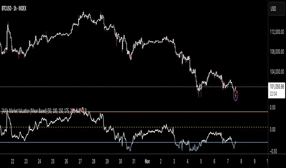
This indicator estimates whether price is overvalued, undervalued, or fairly valued relative to its structural mean across multiple lookback windows. It builds a single normalized oscillator from short-, mid-, and long-term ranges so traders can quickly see when price is stretched away from equilibrium.
This is not a mashup of existing tools. It’s a custom mean-deviation model that aggregates multi-window range positioning into one score.
How it works (concepts)
For each lookback length (13, 25, 30, 50, 100, 200):
Range & midpoint:
Highest high H and lowest low L.
Structural midpoint Mid = (H + L)/2.
Normalized deviation:
Dev = (Close − Mid) / (H − L) → location of price within its own range.
Aggregation:
The oscillator z_struct is the average of the deviations from the five windows.
Result: a smoothed, dimensionless value (roughly −1 to +1 in typical markets) showing multi-horizon displacement from the mean.
Plots & levels
Oscillator (area): z_struct
Reference lines: +0.40 (OB), 0.00 (equilibrium), −0.30 (OS)
Coloring:
Red when z_struct > OB (extended above mean)
Blue when z_struct < OS (extended below mean)
White in between
Suggested use
Mean reversion context: Fade extremes in range-bound conditions; take profits into OB/OS.
Trend awareness: In strong trends, extremes can persist—use levels as exhaustion context rather than standalone entry.
Filter/confirm: Combine with your trend filter or structure tools to time pullbacks and avoid chasing extended moves.
Inputs
Lookbacks: 13, 25, 30, 50, 100, 200
Thresholds: OB = 0.40, OS = −0.30
Notes & limitations
Works on the current symbol/timeframe only; no security() calls and no repainting beyond normal bar completion.
In very tight or flat ranges (H ≈ L), normalized deviations can become sensitive; consider longer windows or higher timeframes.
This is an indicator, not a strategy. No signals are generated; use with risk management.
Originality statement
This script implements an original, multi-window mean-deviation aggregation. It does not replicate a built-in or a public indicator; its purpose is to quantify cross-horizon valuation in a single, normalized measure.
Cerca negli script per "如何用wind搜索股票的发行价和份数"
Egg vs Tennis Ball — Drop/Rebound StrengthEgg vs Tennis Ball — Drop/Rebound Meter
What it does
Classifies selloffs as either:
Eggs — dead‑cat, no bounce
Tennis Balls — fast, decisive rebound
Core features
Detects swing drops from a Pivot High (PH) to a Pivot Low (PL)
Requires drops to be meaningful (volatility‑aware, ATR‑scaled)
Draws a bounce threshold line and a deadline
Decides outcome based on speed and extent of rebound
Tracks scores and win rates across multiple lookback windows
Includes a color‑coded meter and current streak display
Visuals at a glance
Gray diagonal — drop from PH to PL
Teal dotted horizontal — bounce threshold, from PH to the deadline
Solid green — Tennis Ball (bounce line broken before the deadline)
Solid red — Egg (deadline expired before the bounce)
Optional PH / PL labels for clarity
How the decision is made
1) Find pivots — symmetric pivots using Pivot Left / Right; PL confirms after Right bars.
2) Qualify the drop — Drop Size = PH − PL; must be ≥ (Drop Threshold × ATR at PL).
3) Define the bounce line — PL + (Bounce Multiple × Drop Size). 1.00× = full retrace to PH; up to 2.00× for overshoot.
4) Set the deadline — Drop Bars = PL index − PH index; Deadline = Drop Bars × Recovery Factor; timer starts from PH or PL.
5) Resolve — Tennis Ball if price hits the bounce line before the deadline; Egg if the deadline passes first.
Scoring system (−100 to +100)
+100 = perfect Tennis Ball (fastest possible + full overshoot)
−100 = perfect Egg (no recovery)
In between: scored by rebound speed and extent, shaped by your weight settings
Meter Table
Columns (toggle on/off)
All (off by default)
Last N1 (default 5)
Last N2 (default 10)
Last N3 (default 20)
Rows
Tennis / Eggs — counts
% Tennis — win rate
Avg Score — normalized quality from −100 to +100
Streak — overall (not windowed), e.g., +3 = 3 Tennis Balls in a row, −4 = 4 Eggs in a row
Alerts
Tennis Ball – Fast Rebound — triggers when the bounce line is broken in time
Egg – Window Expired — triggers when the deadline passes without a bounce
Inputs
① Drop Detection
Pivot Left / Right
ATR Length
Drop Threshold × ATR
② Bounce Requirement
Bounce Multiple × Drop Size (0.10–2.00×)
③ Timing
Timer Start — PH or PL
Recovery Factor × Drop Bars
Break Trigger — Close or High
④ Display
Show Pivot/Outcome Labels
Line Width
Table Position (corner)
⑤ Meter Columns
Show All (off by default)
Show N1 / N2 / N3 (5, 10, 20 by default)
⑥ Scoring Weights
Tennis — Base, Speed, Extent
Egg — Base, Strength
How to use it
Pick strictness — start with Drop Threshold = 2.0 ATR, Bounce Multiple = 1.0×, Recovery Factor = 3.0×; adjust to timeframe and volatility.
Watch the dotted line — it ends at the deadline; turns solid green (Tennis) if broken in time, solid red (Egg) if it expires.
Read the meter — short windows (5–10) show current behavior; Avg Score captures quality; Streak shows momentum.
Blend with your system — combine with trend filters, volume, or regime detection.
Tips
Close vs High trigger: Close is stricter; High is more responsive.
PH vs PL timer start: PH measures round‑trip; PL measures recovery only.
Increase pivot strength for fewer, more reliable signals.
Higher timeframes generally produce cleaner patterns.
Defaults
Pivot L/R: 5 / 5
ATR Length: 14
Drop Threshold: 2.0× ATR
Bounce Multiple: 1.00×
Recovery Factor: 3.0×
Break Trigger: Close
Windows: Last 5, 10, 20 (All off)
Interpreting results
Tennis‑y: Avg Score +30 to +70, %Tennis > 55%
Mixed: Avg Score near 0
Egg‑y: Avg Score −30 to −80, %Tennis < 45%
Kinetic EMA & Volume with State EngineKinetic EMA & Volume with State Engine (EMVOL)
1. Introduction & Concept
The EMVOL indicator converts a dense family of EMA signals and volume flows into a compact “state engine”. Instead of looking at individual EMA lines or simple crossovers, the script treats each EMA as part of a kinetic vector field and classifies the market into interpretable states:
- Trend direction and strength (from a grid of prime‑period EMAs).
- Volume regime (expansion, contraction, climax, dry‑up).
- Order‑flow bias via delta (buy versus sell volume).
- A combined scenario label that summarises how these three layers interact.
The goal is educational: to help traders see that moving averages and volume become more meaningful when observed as a structure, not as isolated lines. EMVOL is therefore designed as a real‑time teaching tool, not as an automatic signal generator.
2. Volume Settings
Group: “Volume Settings”
A. Calculation Method
- Geometry (Source File) – Default mode.
Buy and sell volume are estimated from each candle’s geometry: the close is compared to the high/low range and the bar’s total volume is split proportionally between buyers and sellers. This approximation works on any TradingView plan and does not require lower‑timeframe data.
- Intrabar (Precise) – Reconstructs buy/sell volume using a lower timeframe via requestUpAndDownVolume(). The script asks TradingView for historical intrabar data (e.g., 15‑second bars) and builds buy/sell volume and delta from that stream. This mode can produce a more accurate view of order flow, but coverage is limited by your account’s history limits and the symbol’s available lower‑timeframe data.
B. Intrabar Resolution (If Precise)
- Intrabar Resolution (If Precise) – Selected only when the calculation method is “Intrabar (Precise)”. It defines which lower timeframe (for example 15S, 30S, 1m) is used to compute up/down volume. Smaller intrabar timeframes may give smoother and more granular deltas, but require more historical depth from the platform.
When “Intrabar (Precise)” is active, the dashboard’s extended section shows the resolution and the number of bars for which precise volume has been successfully retrieved, in the format:
- Mode: Intrabar (15S) – where N is the count of bars with valid high‑resolution volume data.
In Geometry mode this counter simply reflects the processed bars in the current session.
3. Kinetic Vector Settings
Group: “Kinetic Vector”
A. Vector Window
- Vector Window – Controls the temporal smoothing applied to the aggregated vectors (trend, volume, delta, etc.). Internally, each bar’s vector value is averaged with a simple moving window of this length.
- Shorter windows make the state engine more reactive and sensitive to local swings.
- Longer windows make the states more stable and better suited to higher‑timeframe structure.
B. Max Prime Period
- Max Prime Period – Sets the largest prime number used in the EMA grid. The engine builds a family of EMAs on prime lengths (2, 3, 5, 7, …) up to this limit and converts their slopes into angles.
- A higher limit increases the number of long‑horizon EMAs in the grid and makes the vectors sensitive to broader structure.
- A lower limit focuses the analysis on short- and medium‑term behaviour.
C. Price Source
- Price Source – The price series from which the kinetic EMA grid is built (e.g., Close, HLC3, OHLC4). Changing the source modifies the context that the state engine is reading but does not change the core logic.
4. State Engine Settings
Group: “State Engine Settings”
These inputs define how the continuous vectors are translated into discrete states.
A. Trend Thresholds
- Strong Trend Threshold – Value above which the trend vector is treated as “extreme bullish” and below which it is “extreme bearish”.
- Weak Trend Threshold – Inner boundary between neutral and directional conditions.
Roughly:
- |trend| < weak → Neutral trend state.
- weak < |trend| ≤ strong → Bullish/Bearish.
- |trend| > strong → Extreme Bullish/Extreme Bearish.
B. Volume Thresholds
- Volume Climax Threshold – Upper bound at which volume is considered “climax” (unusually expanded participation).
- Volume Expansion Threshold – Boundary for normal expansion versus contraction.
Conceptually:
- Volume above “expansion” indicates increasing activity.
- Volume near or above “climax” marks extreme participation.
- Negative values below the symmetric thresholds map to contraction and extreme dry‑up (liquidity vacuum) states.
C. Delta Thresholds
- Strong Delta Threshold – Cut‑off for extreme buying or selling dominance in delta.
- Weak Delta Threshold – Threshold for mild buy/sell bias versus neutral order flow.
Combined with the sign of the delta vector, these thresholds classify order flow as:
- Extreme Buy, Buy‑Dominant, Neutral, Sell‑Dominant, Extreme Sell.
D. State Hysteresis Bars
- State Hysteresis Bars – Minimum number of bars for which a new state must persist before the engine commits to the change. This prevents the dashboard from flickering during fast spikes and emphasises persistent market behaviour.
- Smaller values switch states quickly; larger values demand more confirmation.
5. Visual Interface
Group: “Visual Interface”
A. Ribbon Base Color
- Ribbon Base Color – Base hue for the multi‑layer EMA ribbon drawn around price. The script plots a dense grid of hidden EMAs and fills the gaps between them to form a semi‑transparent band. Narrow, overlapping bands hint at compression; wider separation hints at dispersion across EMA horizons.
B. Show Dashboard
- Show Dashboard – Toggles the on‑chart table which summarises the current state engine output. Disable this if you only want to keep the EMA ribbon and volume‑based structure on the price chart.
C. Color Theme
- Color Theme – Switch between a dark and light style for the dashboard background and text colours so that the table matches your chart theme.
D. Table Position
- Table Position – Places the dashboard at any corner or edge of the chart (Top / Middle / Bottom × Left / Centre / Right).
E. Table Size
- Table Size – Changes the dashboard’s text size (Tiny, Small, Normal, Large). Use a larger size on high‑resolution screens or when streaming.
F. Show Extended Info
- Show Extended Info – Adds diagnostic rows under the main state summary:
- Mode / Primes / Vector – Shows the current calculation mode (Geometry / Intrabar), the selected intrabar resolution and coverage in bars ( ), how many prime periods are active, and the vector window.
- Values – Displays the current aggregated vectors:
- P: price vector
- V: volume vector
- B: buy‑volume vector
- S: sell‑volume vector
- D: delta vector
Values are bounded between ‑1 and +1.
- Volume Stats – Prints the last bar’s raw buy volume, sell volume and delta as formatted numbers.
- Footer – A final row with the symbol and current time: #SYMBOL | HH:MM.
These extended rows are meant for inspecting how the engine is behaving under the hood while you scroll the chart and compare different assets or timeframes.
6. Language Settings
Group: “Language Settings”
- Select Language – Switches the entire dashboard between English and Turkish.
The underlying calculations and scenario logic are identical; only the labels, titles and comments in the table are translated.
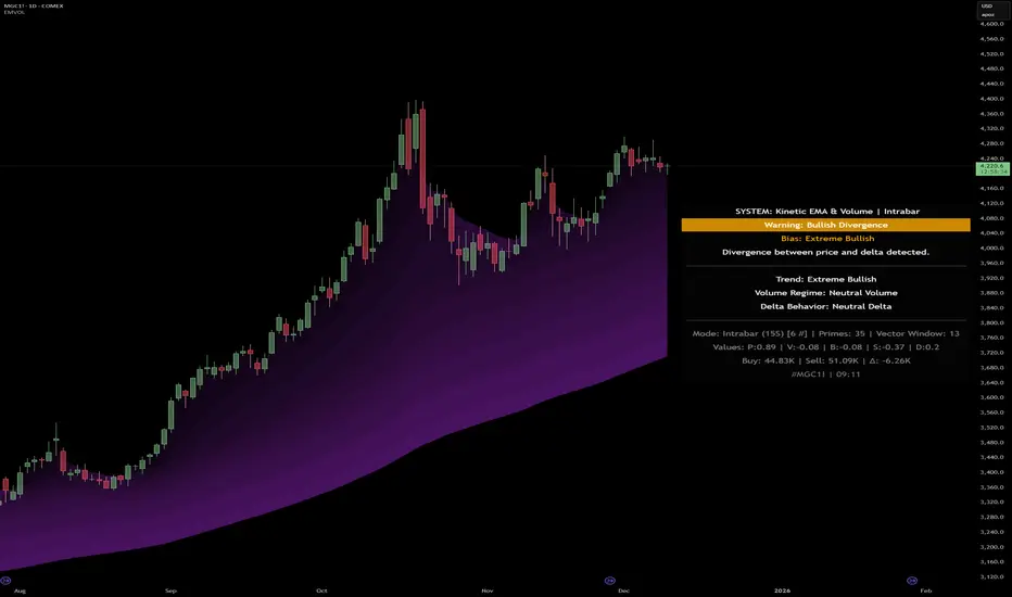
7. Dashboard Structure & Reading Guide
The table summarises the current situation in a few rows:
1. System Header – Shows the script name and the active calculation method (“Geometry” or “Intrabar”).
2. Scenario Title – High‑level description of the current combined scenario (e.g., “Trending Buy Confirmed”, “Sideways Balanced”, “Bull Trap”, “Blow‑Off Top”). The background colour is derived from the scenario family (trending, compression, exhaustion, anomaly, etc.).
3. Bias / Trend Line – States the dominant trend bias derived from the trend vector (Extreme Bullish, Bullish, Neutral, Bearish, Extreme Bearish).
4. Signal / Consideration Line – A short sentence giving qualitative guidance about the current state (for example: continuation risk, exhaustion risk, trap‑like behaviour, or compression). This is deliberately phrased as a consideration, not as a direct trading signal.
5. Trend / Volume / Delta Rows – Three separate rows explain, in plain language, how the trend, volume regime and delta are classified at this bar.
6. Extended Info (optional) – Mode / primes / vector settings, current vector values, and last‑bar volume statistics, as described above.
Together, these rows are meant to be read as a narrative of what price, volume and order‑flow are doing, not as mechanical instructions.
8. State Taxonomy
The state engine organizes market behaviour in three stages.
8.1 Trend States (from the Price Vector)
- Extreme Bullish Trend – The prime‑grid price vector is strongly upward; most EMAs are aligned to the upside.
- Bullish Trend – Upward bias is present, but less extreme.
- Neutral Trend – EMAs are mixed or flat; price is effectively sideways relative to the grid.
- Bearish Trend – Downward bias, with the EMA grid sloping down.
- Extreme Bearish Trend – Strong downside alignment across the grid.
8.2 Volume Regime States (from the Volume Vector)
- Volume Climax (Buy‑Side) – Strong positive volume vector; participation is unusually high in the current direction.
- Volume Expansion – Activity above normal but below the climax threshold.
- Neutral Volume – No major expansion or contraction versus recent history.
- Volume Contraction – Activity is drying up compared with the past.
- Extreme Dry‑Up / Liquidity Vacuum – Very low participation; the market is thin and prone to slippage.
8.3 Delta Behaviour States (from the Delta Vector)
- Extreme Buy Delta – Buying pressure dominates strongly.
- Buy‑Dominant Delta – Buy volume exceeds sell volume, but not at an extreme.
- Neutral Delta – Buy and sell flows are roughly balanced.
- Sell‑Dominant Delta – Selling pressure dominates.
- Extreme Sell Delta – Aggressive, one‑sided selling.
8.4 Combined Scenario State s
EMVOL uses the three base states above to generate a single scenario label. These scenarios are designed to be read as context, not as entry or exit signals.
Trending Scenarios
1. Trending Buy Confirmed
- Bullish or extreme bullish trend, supported by expanding or climax volume and buy‑side delta.
- Educational idea: a healthy uptrend where both participation and order flow agree with the direction.
2. Trending Buy – Weak Volume
- Bullish trend, but volume is neutral, contracting or in dry‑up while delta is still buy‑side.
- Educational idea: price is advancing, yet participation is thinning; trend continuation becomes more fragile.
3. Trending Sell Confirmed
- Bearish or extreme bearish trend, with expanding or climax volume and sell‑side delta.
- Educational idea: strong downtrend with both volume and order‑flow confirmation.
4. Trending Sell – Weak Volume
- Bearish trend, but volume is neutral, contracting or very low while delta remains sell‑side.
- Educational idea: downside continues but with limited participation; vulnerable to short‑covering.
Sideways / Range Scenarios
5. Sideways Balanced
- Neutral trend, neutral delta, neutral volume.
- Classic range environment; low directional edge, suitable for observation and context rather than trend trading.
6. Sideways with Buy Pressure
- Neutral trend, but buy‑side delta is dominant or extreme.
- Range with latent accumulation: price may still appear sideways, but buyers are quietly more active.
7. Sideways with Sell Pressure
- Neutral trend with dominant or extreme sell‑side delta.
- Distribution‑like environment where price chops while sellers are gradually more aggressive.
Exhaustion & Volume Extremes
8. Exhaustion – Buy Risk
- Extreme bullish trend, volume climax and strong buy‑side delta.
- Educational idea: very strong up‑move where both participation and delta are already stretched; risk of exhaustion or blow‑off.
9. Exhaustion – Sell Risk
- Extreme bearish trend, volume dry‑up and strong sell‑side delta.
- Suggests one‑sided selling into increasingly thin liquidity.
10. Volume Climax (Buy)
- Neutral trend, neutral delta, but volume at climax levels.
- Often associated with a “big event” bar where participation spikes without a clear directional commitment.
11. Volume Climax (Sell / Dry‑Up)
- Neutral trend and neutral delta, while the volume vector indicates an extreme dry‑up.
- Highlights a stand‑still episode: very limited interest from both sides, increasing the sensitivity to future impulses.
Divergences
12. Divergence – Bullish Context
- Bullish or extreme bullish trend, but delta has faded back to neutral.
- Price trend continues while order‑flow conviction softens; can precede pauses or complex corrections.
13. Divergence – Bearish Context
- Bearish or extreme bearish trend with a neutral delta.
- Downtrend persists, but selling pressure no longer dominates as clearly.
Consolidation & Compression
14. Consolidation
- Default state when no specific pattern dominates and the market is broadly balanced.
- Educational use: treat this as a “no strong edge” label; focus on structure rather than direction.
15. Breakout Imminent
- Neutral trend with contracting volume.
- Compression phase where energy is building up; often precedes transitions into trending or shock scenarios.
Traps & Hidden Divergences
16. Bull Trap
- Bullish trend, with neutral or contracting volume and sell‑side delta.
- Price appears strong, but order‑flow shifts against it; often seen near fake breakouts or failing rallies.
17. Bear Trap
- Bearish trend, neutral or contracting volume, but buy‑side delta.
- Downtrend “looks” intact, while buyers become more aggressive underneath the surface.
18. Hidden Bullish Divergence
- Bullish trend, contracting volume, but strong buy‑side delta.
- Educational idea: price dips or slows while aggressive buyers step in, often inside an ongoing uptrend.
19. Hidden Bearish Divergence
- Bearish trend, volume expansion and strong sell‑side delta.
- Reinforced downside pressure even if price is temporarily retracing.
Reversal & Transition Patterns
20. Reversal to Bearish
- Neutral trend, volume climax and strong sell‑side delta.
- Suggests that heavy selling appears at the top of a move, turning a previously neutral or rising context into potential downside.
21. Reversal to Bullish
- Neutral trend, extreme volume dry‑up and strong buy‑side delta.
- Often associated with selling exhaustion where buyers start to take control.
22. Indecision Spike
- Neutral trend with extreme volume (climax or dry‑up) but neutral delta.
- Crowd participation changes sharply while order‑flow remains undecided; treat as an informational spike rather than a direction.
Extended Compression & Acceleration
23. Coiling Phase
- Neutral trend, contracting volume, and delta that is neutral or only mildly one‑sided.
- Extended compression where price, volume and delta all contract into a tightly coiled range, often preceding a strong move.
24. Bullish Acceleration
- Bullish trend with volume expansion and strong buy‑side delta.
- Uptrend not only continues but gains kinetic strength; educationally, this illustrates how trend, volume and delta align in the strongest phases of a move.
25. Bearish Acceleration
- Bearish trend with volume expansion and strong sell‑side delta.
- Mirror image of Bullish Acceleration on the downside.
Trend Exhaustion & Climax Reversal
26. Bull Exhaustion
- Bullish or extreme bullish trend, with contraction or dry‑up in volume and buy‑side or neutral delta.
- The move has already travelled far; participation fades while price is still elevated.
27. Bear Exhaustion
- Bearish or extreme bearish trend, with volume climax or contraction and sell‑side or neutral delta.
- Down‑move may be approaching a point where additional selling pressure has diminishing impact.
28. Blow‑Off Top
- Extreme bullish trend, volume climax and extreme buy delta all at once.
- Classic blow‑off behaviour: price, volume and order‑flow are simultaneously stretched in the same direction.
29. Selling Climax Reversal
- Extreme bearish trend with extreme volume dry‑up and extreme sell‑side delta.
- Marks a very aggressive capitulation phase that can precede major rebounds.
Advanced VSA / Anomaly Scenarios
30. Absorption
- Typically neutral trend with expanding or climax volume and extreme delta (either buy or sell).
- Educational focus: large participants are aggressively absorbing liquidity from the opposite side, while price remains relatively contained.
31. Distribution
- Scenario where volume remains elevated while directional conviction weakens and the trend slows.
- Represents potential “selling into strength” or “buying into weakness”, depending on the active side.
32. Liquidity Vacuum
- Combination of thin liquidity (extreme dry‑up) with a directional trend or strong delta.
- Highlights environments where even small orders can move price disproportionately.
33. Anomaly / Shock Event
- Triggered when the vector z‑scores detect rare combinations of price, volume and delta behaviour that deviate from their own historical distribution.
- Intended as a warning label for unusual events rather than a specific tradeable pattern.
9. Educational Usage Notes
- EMVOL does not produce mechanical “buy” or “sell” commands. Instead, it classes each bar into an interpretable state so that traders can study how trends, volume and order‑flow interact over time.
- A common exercise is to overlay your usual EMA crossovers, support/resistance or price patterns and observe which EMVOL scenarios appear around entries, exits, traps and climaxes.
- Because the vectors are normalized (bounded between ‑1 and +1) and then discretized, the same conceptual states can be compared across different symbols and timeframes.
10. Disclaimer & Educational Purpose
This indicator is provided strictly as an educational and analytical tool. Its purpose is to help visualise how price, volume and order‑flow interact; it is not designed to function as a stand‑alone trading system.
Please note:
1. No Automated Strategy – The script does not implement a complete trading strategy. Scenario labels and dashboard messages are descriptive and should not be followed as unconditional entry or exit signals.
2. No Financial Advice – All information produced by this indicator is general market analysis. It must not be interpreted as investment, financial or trading advice, or as a recommendation to buy or sell any instrument.
3. Risk Warning – Trading and investing involve substantial risk, including the risk of loss. Always perform your own analysis, use appropriate position sizing and risk management, and consult a qualified professional if needed. You are solely responsible for any decisions made using this tool.
4. Data Precision & Platform Limits – The “Intrabar (Precise)” mode depends on the availability of high‑resolution historical data at the chosen intrabar timeframe. If your TradingView plan or the symbol’s history does not provide sufficient depth, this mode may only partially cover the visible chart. In such cases, consider switching to “Geometry (Source File)” for a fully populated view.
NY 4H Wyckoff State Machine [CHE] NY 4H Wyckoff State Machine — Full (Re-Entry, Breakout, Wick, Re-Accum/Distrib, Dynamic Table) — One-Candle Wyckoff Re-Entry (OCWR)
Summary
OCWR operationalizes a one-candle session workflow: mark the first four-hour New York candle, fix its high and low as the session range when the window closes, and drive entries through a Wyckoff-style state machine on intraday bars. The script adds an ATR-scaled buffer around the range and requires multi-bar acceptance before treating breaks or re-entries as valid. Optional wick-cluster evidence, a proximity retest, and simple volume or RSI gates increase selectivity. Background tints expose regimes, shapes mark events, a dynamic table explains the current state, and hidden plots supply alert payloads. The design reduces random flips and makes state transitions auditable without higher-timeframe calls.
Origin and name
Method name: One-Candle Wyckoff Re-Entry (OCWR)
Transcript origin: The source idea is a “stupid simple one-candle scalping” routine: mark the first New York four-hour candle (commonly between one and five in the morning New York time), drop to five minutes, observe accumulation inside, wait for a manipulation move outside, then trade the re-entry back inside. Stops go beyond the excursion extreme; targets are either a fixed reward multiple or the opposite side of the range. Preference is given to several manipulation candles. This indicator codifies that workflow with explicit states, acceptance counters, buffers, and optional quality filters. Any external performance claims are not part of the code.
Motivation: Why this design?
Session levels are widely respected, yet single-bar breaches around them are noisy. OCWR separates range discovery from trade logic. It locks the range at the end of the window, applies an ATR-scaled buffer to ignore marginal oversteps, and requires acceptance over several bars for breaks and re-entries. Wick evidence and optional retest proximity help confirm that an excursion likely cleared liquidity rather than launched a trend. This yields cleaner transitions from test to commitment.
What’s different vs. standard approaches?
Baseline: Static session lines or one-shot Wyckoff tags without process control.
Architecture: Dual long and short state machines; ATR-buffered edges; multi-bar acceptance for breaks and re-entries; optional wick dominance and cluster checks; optional retest tolerance; direct and opposite breakout paths; cooldown after fires; distribution timeout; dynamic table with highlighted row.
Practical effect: Fewer single-bar head-fakes, clearer hand-offs, and on-chart explanations of the machine’s view.
Wyckoff structure by example — OCWR on five minutes
One-candle setup:
On the four-hour chart, mark the first New York candle’s high and low, then switch to five minutes. Solid lines show the fixed range; dashed lines show ATR-buffered edges.
Long path (verbal mapping):
Phase A, Stopping Action: Price stabilizes inside the range.
Phase B, Consolidation: Sustained balance while the window is closed and after the range is fixed.
Phase C, Test (Spring): Excursion below the buffered low with preference for several outside bars and dominant lower wicks, then a return inside.
Re-entry acceptance: A required run of inside bars validates the test.
Phase D, Breakout to Markup: Long signal fires; stop beyond the excursion extreme; objective is the opposite range or a fixed reward multiple.
Phase E, Trend (Markup) and Re-Accumulation: Advance continues until target, stop, confirmation back against the box, or timeout. A pause inside trend may register as re-accumulation.
Short path mirrors the above: A UTAD-style move forms above the buffered high, then re-entry leads to Markdown and possible re-distribution.
Variant map (verbal):
Accumulation after a downtrend: with Spring and Test, or without Spring; both proceed to Markup and may pause in Re-Accumulation.
Distribution after an uptrend: with UTAD and Test, or without UTAD; both proceed to Markdown and may pause in Re-Distribution.
Note: Phases A through E occur within each variant and are not separate variants.
How it works (technical)
Session window: A configurable four-hour New York window records its high and low. At window end, the bounds are fixed for the session.
ATR buffer: A margin above and below the fixed range discourages triggers from tiny oversteps.
Inside and outside: Users choose close-based or wick-based detection. Overshoot requirements are expressed verbally as a fraction of the range with an optional absolute minimum.
Manipulation tracking: The machine counts bars spent outside and records the side extreme.
Re-entry acceptance: After a return inside, a specified number of inside bars must print before acceptance.
Direct and opposite breakouts: Direct breakouts from accumulation and opposite breakouts after manipulation are supported, subject to acceptance and optional filters.
Targets and exits: Choose the opposite boundary or a fixed reward multiple. Distribution ends on target, stop, confirmation back against the range, or timeout.
Context filters (optional): Volume above a scaled SMA, RSI thresholds, and a trend SMA for simple regime context.
Diagnostics: Background tints for regimes; arrows for re-entries; triangles for breakouts; table with row highlights; hidden plots for alert values.
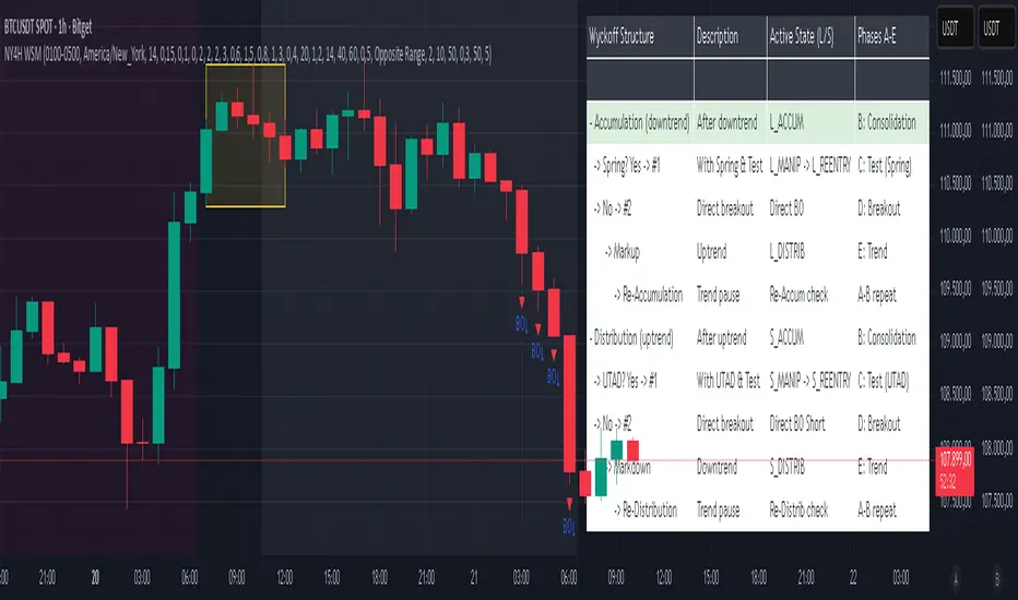
Central table (Wyckoff console)
The table sits top-right and explains the machine’s stance. Columns: Structure label, plain-English description, active state pair for long and short, and human phase tags. Rows: Start and range building; accumulation branch with Spring and Test as well as direct breakout; Markup and re-accumulation; distribution branch with UTAD and Test as well as direct short breakout; Markdown and re-distribution. Only the active state cell is rewritten each last bar, for example “L_ACCUM slash S_ACCUM”. Row highlighting is context-aware: accumulation, Spring or UTAD, breakout, Markup or Markdown, and re-accumulation or re-distribution checks can highlight independently so users see simultaneous conditions. The table is created once, updated only on the last bar for efficiency, and functions as a read-only console to audit why a signal fired and where the path currently sits.
Parameter Guide
Session window and time zone: First four hours of New York by default; time zone “America/New_York”.
ATR length and buffer factor: Control buffer size; larger reduces sensitivity, smaller reacts faster.
Minimum overshoot (fraction and absolute): Demand meaningful extension beyond the buffer.
Break mode: Close-based is stricter; wick-based is more reactive.
Acceptance counts: Separate counts for break, re-entry, and opposite breakout; higher values reduce noise.
Minimum bars outside: Ensures manipulation is not a single spike.
Wick detection and clusters (optional): Dominance thresholds and cluster size within a short window.
Retest required and tolerance (optional): Gate re-entry by proximity to the buffered edge.
Volume and RSI filters (optional): Simple gates on activity and momentum.
TP mode and reward multiple: Opposite range or fixed multiple.
Cooldown and distribution timeout: Rate-limit signals and prevent endless distribution.
Visualization toggles: Background phases, labels, table, and helper lines.
Reading & Interpretation
Solid lines are the fixed session bounds; dashed lines are buffers. Backgrounds tint accumulation, manipulation, and distribution. Arrows show accepted re-entries; triangles show direct or opposite breakouts. Labels can summarize entry, stop, target, and risk. The table highlights the active row and the current state pair.
Practical Workflows & Combinations
OCWR baseline: Each morning, mark the New York four-hour candle, move to five minutes, prefer multi-bar manipulation outside, then wait for a qualified re-entry inside. Stop beyond the excursion extreme. Target the opposite range for conservative management or a fixed multiple for uniform sizing.
Trend following: Favor direct breakouts with trend alignment and no contradictory wick evidence.
Quality control: When noise rises, increase acceptance, raise the buffer factor, enable retest, and require wick clusters.
Discretionary confluences: Fair-value gaps and trend lines can be added by the user; they are not computed by this script.
Behavior, Constraints & Performance
Closed-bar confirmation is recommended when you require finality; live-bar conditions can change until close. The script does not call higher-timeframe data. It uses arrays, lines, labels, boxes, and a table; maximum bars back is five thousand; table updates are last-bar only. Known limits include compressed buffers in quiet sessions, unreliable wick evidence in thin markets, and session misalignment if the platform time zone is not New York.
Sensible Defaults & Quick Tuning
Start with ATR length fourteen, buffer factor near zero point fifteen, overshoot fraction near zero point ten, acceptance counts of two, minimum outside duration three, retest required on.
Too many flips: increase acceptance, raise buffer, enable retest, and tighten wick thresholds.
Too slow: reduce acceptance, lower buffer, switch to wick-based breaks, disable retest.
Noisy wicks: increase minimum wick ratio and cluster size, or disable wick detection.
What this indicator is—and isn’t
A session-anchored visualization and signal layer that formalizes a Wyckoff-style re-entry and breakout workflow derived from a single four-hour New York candle. It is not predictive and not a complete trading system. Use with structure analysis, risk controls, and position management.
Disclaimer
The content provided, including all code and materials, is strictly for educational and informational purposes only. It is not intended as, and should not be interpreted as, financial advice, a recommendation to buy or sell any financial instrument, or an offer of any financial product or service. All strategies, tools, and examples discussed are provided for illustrative purposes to demonstrate coding techniques and the functionality of Pine Script within a trading context.
Any results from strategies or tools provided are hypothetical, and past performance is not indicative of future results. Trading and investing involve high risk, including the potential loss of principal, and may not be suitable for all individuals. Before making any trading decisions, please consult with a qualified financial professional to understand the risks involved.
By using this script, you acknowledge and agree that any trading decisions are made solely at your discretion and risk.
Do not use this indicator on Heikin-Ashi, Renko, Kagi, Point-and-Figure, or Range charts, as these chart types can produce unrealistic results for signal markers and alerts.
Best regards and happy trading
Chervolino
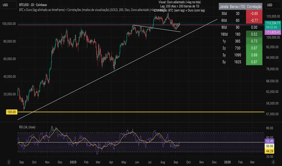
Bitcoin vs. Gold correlation with lagBTC vs Gold (Lag) + Correlation — multi-timeframe, publication notes
What it does
Plots Gold on the same chart as Bitcoin, with a configurable lead/lag.
Lets you choose how the series is displayed:
Gold shifted forward (+lag on chart) — shows gold ahead of BTC on the time axis (visual offset).
Gold aligned to BTC (gold lag) — standard alignment; gold is lagged for calculation and plotted in place.
BTC 200D Lag (BTC shifted forward) — visualizes BTC shifted forward (like popular “BTC 200D Lag” charts).
Computes Pearson correlations between BTC (no lag) and Gold (with lag) over multiple lookback windows equivalent to:
30d, 60d, 90d, 180d, 365d, 2y (730d), 3y (1095d), 5y (1825d).
Shows a table with the correlation values, automatically scaled to the current timeframe.
Why this is useful
A common macro claim is that BTC tends to follow Gold with a delay (e.g., ~200 trading days). This tool lets you:
Visually advance Gold (or BTC) to see that lead-lag relationship on the chart.
Quantify the relationship with rolling correlations.
Switch timeframes (D/W/M/…): everything automatically stays in sync.
Quick start
Open a BTC chart (any exchange).
Add the indicator.
Set Gold symbol (default TVC:GOLD; alternatives: OANDA:XAUUSD, COMEX:GC1!, etc.).
Choose Lag value and Lag unit (Days/Weeks/Months/Years/Bars).
Pick Visual Mode:
To mirror those “BTC 200D Lag” posts: choose “BTC 200D Lag (BTC shifted forward)” with 200 Days.
To view Gold 200D ahead of BTC: select “Gold shifted forward (+lag on chart)” with 200 Days.
Keep Rebase to 100 ON for an apples-to-apples visual scale. (You can move the study to the left price scale if needed.)
Inputs
Gold symbol: external series to pair with BTC.
Lag value: numeric value.
Lag unit: Days, Weeks, Months (≈30d), Years (≈365d), or direct Bars.
Visual mode:
Gold shifted forward (+lag on chart) → gold is offset to the right by the lag (visual only).
Gold aligned to BTC (gold lag) → standard plot (no visual offset); correlations still use lagged gold.
BTC 200D Lag (BTC shifted forward) → BTC is offset to the right by the lag (visual only).
Rebase to 100 (visual): rescales each series to 100 on its first valid bar for clearer comparison.
Show gold without lag (debug): optional reference line.
Show price tag for gold (lag): toggles the track price label.
Timeframe handling
The study uses the current chart timeframe for both BTC and Gold (timeframe.period).
Lag in time units (Days/Weeks/Months/Years) is internally converted to an integer number of bars of the active timeframe (using timeframe.in_seconds).
Example: on W (weekly), 200 days ≈ 29 bars.
On intraday timeframes, days are converted proportionally.
Correlation math
Correlation = ta.correlation(BTC, Gold_lagged, length_in_bars)
Lookback lengths are the bar-equivalents of 30/60/90/180/365/730/1095/1825 days in the active timeframe.
Important: correlations are computed on prices (not returns). If you prefer returns-based correlation (often more statistically robust), duplicate the script and replace price inputs with change(close) or ta.roc(close, 1).
Reading the table
Window: nominal day label (e.g., 30d, 1y, 5y).
Bars (TF): how many bars that window equals on the current timeframe.
Correlation: Pearson coefficient . Background tint shows intensity and sign.
Tips & caveats
Visual offsets (offset=) move series on screen only; they don’t affect the math. The math always uses BTC (no lag) × Gold (lagged).
With large lags on high timeframes, early bars will be na (normal). Scroll forward / reduce lag.
If your Gold feed doesn’t load, try an alternative symbol that your plan supports.
Rebase to 100 helps visibility when BTC ($100k) and Gold ($2k) share a scale.
Months/Years use 30/365-day approximations. For exact control, use Days or Bars.
Correlations on very short lengths or sparse data can be unstable; consider the longer windows for sturdier signals.
This is a visual/analytical tool, not a trading signal. Always apply independent risk management.
Suggested setups
Replicate “BTC 200D Lag” charts:
Visual Mode: BTC 200D Lag (BTC shifted forward)
Lag: 200 Days
Rebase: ON
Gold leads BTC (Gold ahead):
Visual Mode: Gold shifted forward (+lag on chart)
Lag: 200 Days
Rebase: ON
Compatibility: Pine v6, overlay study.
Best with: BTCUSD (any exchange) + a reliable Gold feed.
Author’s note: Lead-lag relationships are not stable over time; treat correlations as descriptive, not predictive.
ATAI Volume analysis with price action V 1.00ATAI Volume Analysis with Price Action
1. Introduction
1.1 Overview
ATAI Volume Analysis with Price Action is a composite indicator designed for TradingView. It combines per‑side volume data —that is, how much buying and selling occurs during each bar—with standard price‑structure elements such as swings, trend lines and support/resistance. By blending these elements the script aims to help a trader understand which side is in control, whether a breakout is genuine, when markets are potentially exhausted and where liquidity providers might be active.
The indicator is built around TradingView’s up/down volume feed accessed via the TradingView/ta/10 library. The following excerpt from the script illustrates how this feed is configured:
import TradingView/ta/10 as tvta
// Determine lower timeframe string based on user choice and chart resolution
string lower_tf_breakout = use_custom_tf_input ? custom_tf_input :
timeframe.isseconds ? "1S" :
timeframe.isintraday ? "1" :
timeframe.isdaily ? "5" : "60"
// Request up/down volume (both positive)
= tvta.requestUpAndDownVolume(lower_tf_breakout)
Lower‑timeframe selection. If you do not specify a custom lower timeframe, the script chooses a default based on your chart resolution: 1 second for second charts, 1 minute for intraday charts, 5 minutes for daily charts and 60 minutes for anything longer. Smaller intervals provide a more precise view of buyer and seller flow but cover fewer bars. Larger intervals cover more history at the cost of granularity.
Tick vs. time bars. Many trading platforms offer a tick / intrabar calculation mode that updates an indicator on every trade rather than only on bar close. Turning on one‑tick calculation will give the most accurate split between buy and sell volume on the current bar, but it typically reduces the amount of historical data available. For the highest fidelity in live trading you can enable this mode; for studying longer histories you might prefer to disable it. When volume data is completely unavailable (some instruments and crypto pairs), all modules that rely on it will remain silent and only the price‑structure backbone will operate.
Figure caption, Each panel shows the indicator’s info table for a different volume sampling interval. In the left chart, the parentheses “(5)” beside the buy‑volume figure denote that the script is aggregating volume over five‑minute bars; the center chart uses “(1)” for one‑minute bars; and the right chart uses “(1T)” for a one‑tick interval. These notations tell you which lower timeframe is driving the volume calculations. Shorter intervals such as 1 minute or 1 tick provide finer detail on buyer and seller flow, but they cover fewer bars; longer intervals like five‑minute bars smooth the data and give more history.
Figure caption, The values in parentheses inside the info table come directly from the Breakout — Settings. The first row shows the custom lower-timeframe used for volume calculations (e.g., “(1)”, “(5)”, or “(1T)”)
2. Price‑Structure Backbone
Even without volume, the indicator draws structural features that underpin all other modules. These features are always on and serve as the reference levels for subsequent calculations.
2.1 What it draws
• Pivots: Swing highs and lows are detected using the pivot_left_input and pivot_right_input settings. A pivot high is identified when the high recorded pivot_right_input bars ago exceeds the highs of the preceding pivot_left_input bars and is also higher than (or equal to) the highs of the subsequent pivot_right_input bars; pivot lows follow the inverse logic. The indicator retains only a fixed number of such pivot points per side, as defined by point_count_input, discarding the oldest ones when the limit is exceeded.
• Trend lines: For each side, the indicator connects the earliest stored pivot and the most recent pivot (oldest high to newest high, and oldest low to newest low). When a new pivot is added or an old one drops out of the lookback window, the line’s endpoints—and therefore its slope—are recalculated accordingly.
• Horizontal support/resistance: The highest high and lowest low within the lookback window defined by length_input are plotted as horizontal dashed lines. These serve as short‑term support and resistance levels.
• Ranked labels: If showPivotLabels is enabled the indicator prints labels such as “HH1”, “HH2”, “LL1” and “LL2” near each pivot. The ranking is determined by comparing the price of each stored pivot: HH1 is the highest high, HH2 is the second highest, and so on; LL1 is the lowest low, LL2 is the second lowest. In the case of equal prices the newer pivot gets the better rank. Labels are offset from price using ½ × ATR × label_atr_multiplier, with the ATR length defined by label_atr_len_input. A dotted connector links each label to the candle’s wick.
2.2 Key settings
• length_input: Window length for finding the highest and lowest values and for determining trend line endpoints. A larger value considers more history and will generate longer trend lines and S/R levels.
• pivot_left_input, pivot_right_input: Strictness of swing confirmation. Higher values require more bars on either side to form a pivot; lower values create more pivots but may include minor swings.
• point_count_input: How many pivots are kept in memory on each side. When new pivots exceed this number the oldest ones are discarded.
• label_atr_len_input and label_atr_multiplier: Determine how far pivot labels are offset from the bar using ATR. Increasing the multiplier moves labels further away from price.
• Styling inputs for trend lines, horizontal lines and labels (color, width and line style).
Figure caption, The chart illustrates how the indicator’s price‑structure backbone operates. In this daily example, the script scans for bars where the high (or low) pivot_right_input bars back is higher (or lower) than the preceding pivot_left_input bars and higher or lower than the subsequent pivot_right_input bars; only those bars are marked as pivots.
These pivot points are stored and ranked: the highest high is labelled “HH1”, the second‑highest “HH2”, and so on, while lows are marked “LL1”, “LL2”, etc. Each label is offset from the price by half of an ATR‑based distance to keep the chart clear, and a dotted connector links the label to the actual candle.
The red diagonal line connects the earliest and latest stored high pivots, and the green line does the same for low pivots; when a new pivot is added or an old one drops out of the lookback window, the end‑points and slopes adjust accordingly. Dashed horizontal lines mark the highest high and lowest low within the current lookback window, providing visual support and resistance levels. Together, these elements form the structural backbone that other modules reference, even when volume data is unavailable.
3. Breakout Module
3.1 Concept
This module confirms that a price break beyond a recent high or low is supported by a genuine shift in buying or selling pressure. It requires price to clear the highest high (“HH1”) or lowest low (“LL1”) and, simultaneously, that the winning side shows a significant volume spike, dominance and ranking. Only when all volume and price conditions pass is a breakout labelled.
3.2 Inputs
• lookback_break_input : This controls the number of bars used to compute moving averages and percentiles for volume. A larger value smooths the averages and percentiles but makes the indicator respond more slowly.
• vol_mult_input : The “spike” multiplier; the current buy or sell volume must be at least this multiple of its moving average over the lookback window to qualify as a breakout.
• rank_threshold_input (0–100) : Defines a volume percentile cutoff: the current buyer/seller volume must be in the top (100−threshold)%(100−threshold)% of all volumes within the lookback window. For example, if set to 80, the current volume must be in the top 20 % of the lookback distribution.
• ratio_threshold_input (0–1) : Specifies the minimum share of total volume that the buyer (for a bullish breakout) or seller (for bearish) must hold on the current bar; the code also requires that the cumulative buyer volume over the lookback window exceeds the seller volume (and vice versa for bearish cases).
• use_custom_tf_input / custom_tf_input : When enabled, these inputs override the automatic choice of lower timeframe for up/down volume; otherwise the script selects a sensible default based on the chart’s timeframe.
• Label appearance settings : Separate options control the ATR-based offset length, offset multiplier, label size and colors for bullish and bearish breakout labels, as well as the connector style and width.
3.3 Detection logic
1. Data preparation : Retrieve per‑side volume from the lower timeframe and take absolute values. Build rolling arrays of the last lookback_break_input values to compute simple moving averages (SMAs), cumulative sums and percentile ranks for buy and sell volume.
2. Volume spike: A spike is flagged when the current buy (or, in the bearish case, sell) volume is at least vol_mult_input times its SMA over the lookback window.
3. Dominance test: The buyer’s (or seller’s) share of total volume on the current bar must meet or exceed ratio_threshold_input. In addition, the cumulative sum of buyer volume over the window must exceed the cumulative sum of seller volume for a bullish breakout (and vice versa for bearish). A separate requirement checks the sign of delta: for bullish breakouts delta_breakout must be non‑negative; for bearish breakouts it must be non‑positive.
4. Percentile rank: The current volume must fall within the top (100 – rank_threshold_input) percent of the lookback distribution—ensuring that the spike is unusually large relative to recent history.
5. Price test: For a bullish signal, the closing price must close above the highest pivot (HH1); for a bearish signal, the close must be below the lowest pivot (LL1).
6. Labeling: When all conditions above are satisfied, the indicator prints “Breakout ↑” above the bar (bullish) or “Breakout ↓” below the bar (bearish). Labels are offset using half of an ATR‑based distance and linked to the candle with a dotted connector.
Figure caption, (Breakout ↑ example) , On this daily chart, price pushes above the red trendline and the highest prior pivot (HH1). The indicator recognizes this as a valid breakout because the buyer‑side volume on the lower timeframe spikes above its recent moving average and buyers dominate the volume statistics over the lookback period; when combined with a close above HH1, this satisfies the breakout conditions. The “Breakout ↑” label appears above the candle, and the info table highlights that up‑volume is elevated relative to its 11‑bar average, buyer share exceeds the dominance threshold and money‑flow metrics support the move.
Figure caption, In this daily example, price breaks below the lowest pivot (LL1) and the lower green trendline. The indicator identifies this as a bearish breakout because sell‑side volume is sharply elevated—about twice its 11‑bar average—and sellers dominate both the bar and the lookback window. With the close falling below LL1, the script triggers a Breakout ↓ label and marks the corresponding row in the info table, which shows strong down volume, negative delta and a seller share comfortably above the dominance threshold.
4. Market Phase Module (Volume Only)
4.1 Concept
Not all markets trend; many cycle between periods of accumulation (buying pressure building up), distribution (selling pressure dominating) and neutral behavior. This module classifies the current bar into one of these phases without using ATR , relying solely on buyer and seller volume statistics. It looks at net flows, ratio changes and an OBV‑like cumulative line with dual‑reference (1‑ and 2‑bar) trends. The result is displayed both as on‑chart labels and in a dedicated row of the info table.
4.2 Inputs
• phase_period_len: Number of bars over which to compute sums and ratios for phase detection.
• phase_ratio_thresh : Minimum buyer share (for accumulation) or minimum seller share (for distribution, derived as 1 − phase_ratio_thresh) of the total volume.
• strict_mode: When enabled, both the 1‑bar and 2‑bar changes in each statistic must agree on the direction (strict confirmation); when disabled, only one of the two references needs to agree (looser confirmation).
• Color customisation for info table cells and label styling for accumulation and distribution phases, including ATR length, multiplier, label size, colors and connector styles.
• show_phase_module: Toggles the entire phase detection subsystem.
• show_phase_labels: Controls whether on‑chart labels are drawn when accumulation or distribution is detected.
4.3 Detection logic
The module computes three families of statistics over the volume window defined by phase_period_len:
1. Net sum (buyers minus sellers): net_sum_phase = Σ(buy) − Σ(sell). A positive value indicates a predominance of buyers. The code also computes the differences between the current value and the values 1 and 2 bars ago (d_net_1, d_net_2) to derive up/down trends.
2. Buyer ratio: The instantaneous ratio TF_buy_breakout / TF_tot_breakout and the window ratio Σ(buy) / Σ(total). The current ratio must exceed phase_ratio_thresh for accumulation or fall below 1 − phase_ratio_thresh for distribution. The first and second differences of the window ratio (d_ratio_1, d_ratio_2) determine trend direction.
3. OBV‑like cumulative net flow: An on‑balance volume analogue obv_net_phase increments by TF_buy_breakout − TF_sell_breakout each bar. Its differences over the last 1 and 2 bars (d_obv_1, d_obv_2) provide trend clues.
The algorithm then combines these signals:
• For strict mode , accumulation requires: (a) current ratio ≥ threshold, (b) cumulative ratio ≥ threshold, (c) both ratio differences ≥ 0, (d) net sum differences ≥ 0, and (e) OBV differences ≥ 0. Distribution is the mirror case.
• For loose mode , it relaxes the directional tests: either the 1‑ or the 2‑bar difference needs to agree in each category.
If all conditions for accumulation are satisfied, the phase is labelled “Accumulation” ; if all conditions for distribution are satisfied, it’s labelled “Distribution” ; otherwise the phase is “Neutral” .
4.4 Outputs
• Info table row : Row 8 displays “Market Phase (Vol)” on the left and the detected phase (Accumulation, Distribution or Neutral) on the right. The text colour of both cells matches a user‑selectable palette (typically green for accumulation, red for distribution and grey for neutral).
• On‑chart labels : When show_phase_labels is enabled and a phase persists for at least one bar, the module prints a label above the bar ( “Accum” ) or below the bar ( “Dist” ) with a dashed or dotted connector. The label is offset using ATR based on phase_label_atr_len_input and phase_label_multiplier and is styled according to user preferences.
Figure caption, The chart displays a red “Dist” label above a particular bar, indicating that the accumulation/distribution module identified a distribution phase at that point. The detection is based on seller dominance: during that bar, the net buyer-minus-seller flow and the OBV‑style cumulative flow were trending down, and the buyer ratio had dropped below the preset threshold. These conditions satisfy the distribution criteria in strict mode. The label is placed above the bar using an ATR‑based offset and a dashed connector. By the time of the current bar in the screenshot, the phase indicator shows “Neutral” in the info table—signaling that neither accumulation nor distribution conditions are currently met—yet the historical “Dist” label remains to mark where the prior distribution phase began.
Figure caption, In this example the market phase module has signaled an Accumulation phase. Three bars before the current candle, the algorithm detected a shift toward buyers: up‑volume exceeded its moving average, down‑volume was below average, and the buyer share of total volume climbed above the threshold while the on‑balance net flow and cumulative ratios were trending upwards. The blue “Accum” label anchored below that bar marks the start of the phase; it remains on the chart because successive bars continue to satisfy the accumulation conditions. The info table confirms this: the “Market Phase (Vol)” row still reads Accumulation, and the ratio and sum rows show buyers dominating both on the current bar and across the lookback window.
5. OB/OS Spike Module
5.1 What overbought/oversold means here
In many markets, a rapid extension up or down is often followed by a period of consolidation or reversal. The indicator interprets overbought (OB) conditions as abnormally strong selling risk at or after a price rally and oversold (OS) conditions as unusually strong buying risk after a decline. Importantly, these are not direct trade signals; rather they flag areas where caution or contrarian setups may be appropriate.
5.2 Inputs
• minHits_obos (1–7): Minimum number of oscillators that must agree on an overbought or oversold condition for a label to print.
• syncWin_obos: Length of a small sliding window over which oscillator votes are smoothed by taking the maximum count observed. This helps filter out choppy signals.
• Volume spike criteria: kVolRatio_obos (ratio of current volume to its SMA) and zVolThr_obos (Z‑score threshold) across volLen_obos. Either threshold can trigger a spike.
• Oscillator toggles and periods: Each of RSI, Stochastic (K and D), Williams %R, CCI, MFI, DeMarker and Stochastic RSI can be independently enabled; their periods are adjustable.
• Label appearance: ATR‑based offset, size, colors for OB and OS labels, plus connector style and width.
5.3 Detection logic
1. Directional volume spikes: Volume spikes are computed separately for buyer and seller volumes. A sell volume spike (sellVolSpike) flags a potential OverBought bar, while a buy volume spike (buyVolSpike) flags a potential OverSold bar. A spike occurs when the respective volume exceeds kVolRatio_obos times its simple moving average over the window or when its Z‑score exceeds zVolThr_obos.
2. Oscillator votes: For each enabled oscillator, calculate its overbought and oversold state using standard thresholds (e.g., RSI ≥ 70 for OB and ≤ 30 for OS; Stochastic %K/%D ≥ 80 for OB and ≤ 20 for OS; etc.). Count how many oscillators vote for OB and how many vote for OS.
3. Minimum hits: Apply the smoothing window syncWin_obos to the vote counts using a maximum‑of‑last‑N approach. A candidate bar is only considered if the smoothed OB hit count ≥ minHits_obos (for OverBought) or the smoothed OS hit count ≥ minHits_obos (for OverSold).
4. Tie‑breaking: If both OverBought and OverSold spike conditions are present on the same bar, compare the smoothed hit counts: the side with the higher count is selected; ties default to OverBought.
5. Label printing: When conditions are met, the bar is labelled as “OverBought X/7” above the candle or “OverSold X/7” below it. “X” is the number of oscillators confirming, and the bracket lists the abbreviations of contributing oscillators. Labels are offset from price using half of an ATR‑scaled distance and can optionally include a dotted or dashed connector line.
Figure caption, In this chart the overbought/oversold module has flagged an OverSold signal. A sell‑off from the prior highs brought price down to the lower trend‑line, where the bar marked “OverSold 3/7 DeM” appears. This label indicates that on that bar the module detected a buy‑side volume spike and that at least three of the seven enabled oscillators—in this case including the DeMarker—were in oversold territory. The label is printed below the candle with a dotted connector, signaling that the market may be temporarily exhausted on the downside. After this oversold print, price begins to rebound towards the upper red trend‑line and higher pivot levels.
Figure caption, This example shows the overbought/oversold module in action. In the left‑hand panel you can see the OB/OS settings where each oscillator (RSI, Stochastic, Williams %R, CCI, MFI, DeMarker and Stochastic RSI) can be enabled or disabled, and the ATR length and label offset multiplier adjusted. On the chart itself, price has pushed up to the descending red trendline and triggered an “OverBought 3/7” label. That means the sell‑side volume spiked relative to its average and three out of the seven enabled oscillators were in overbought territory. The label is offset above the candle by half of an ATR and connected with a dashed line, signaling that upside momentum may be overextended and a pause or pullback could follow.
6. Buyer/Seller Trap Module
6.1 Concept
A bull trap occurs when price appears to break above resistance, attracting buyers, but fails to sustain the move and quickly reverses, leaving a long upper wick and trapping late entrants. A bear trap is the opposite: price breaks below support, lures in sellers, then snaps back, leaving a long lower wick and trapping shorts. This module detects such traps by looking for price structure sweeps, order‑flow mismatches and dominance reversals. It uses a scoring system to differentiate risk from confirmed traps.
6.2 Inputs
• trap_lookback_len: Window length used to rank extremes and detect sweeps.
• trap_wick_threshold: Minimum proportion of a bar’s range that must be wick (upper for bull traps, lower for bear traps) to qualify as a sweep.
• trap_score_risk: Minimum aggregated score required to flag a trap risk. (The code defines a trap_score_confirm input, but confirmation is actually based on price reversal rather than a separate score threshold.)
• trap_confirm_bars: Maximum number of bars allowed for price to reverse and confirm the trap. If price does not reverse in this window, the risk label will expire or remain unconfirmed.
• Label settings: ATR length and multiplier for offsetting, size, colours for risk and confirmed labels, and connector style and width. Separate settings exist for bull and bear traps.
• Toggle inputs: show_trap_module and show_trap_labels enable the module and control whether labels are drawn on the chart.
6.3 Scoring logic
The module assigns points to several conditions and sums them to determine whether a trap risk is present. For bull traps, the score is built from the following (bear traps mirror the logic with highs and lows swapped):
1. Sweep (2 points): Price trades above the high pivot (HH1) but fails to close above it and leaves a long upper wick at least trap_wick_threshold × range. For bear traps, price dips below the low pivot (LL1), fails to close below and leaves a long lower wick.
2. Close break (1 point): Price closes beyond HH1 or LL1 without leaving a long wick.
3. Candle/delta mismatch (2 points): The candle closes bullish yet the order flow delta is negative or the seller ratio exceeds 50%, indicating hidden supply. Conversely, a bearish close with positive delta or buyer dominance suggests hidden demand.
4. Dominance inversion (2 points): The current bar’s buyer volume has the highest rank in the lookback window while cumulative sums favor sellers, or vice versa.
5. Low‑volume break (1 point): Price crosses the pivot but total volume is below its moving average.
The total score for each side is compared to trap_score_risk. If the score is high enough, a “Bull Trap Risk” or “Bear Trap Risk” label is drawn, offset from the candle by half of an ATR‑scaled distance using a dashed outline. If, within trap_confirm_bars, price reverses beyond the opposite level—drops back below the high pivot for bull traps or rises above the low pivot for bear traps—the label is upgraded to a solid “Bull Trap” or “Bear Trap” . In this version of the code, there is no separate score threshold for confirmation: the variable trap_score_confirm is unused; confirmation depends solely on a successful price reversal within the specified number of bars.
Figure caption, In this example the trap module has flagged a Bear Trap Risk. Price initially breaks below the most recent low pivot (LL1), but the bar closes back above that level and leaves a long lower wick, suggesting a failed push lower. Combined with a mismatch between the candle direction and the order flow (buyers regain control) and a reversal in volume dominance, the aggregate score exceeds the risk threshold, so a dashed “Bear Trap Risk” label prints beneath the bar. The green and red trend lines mark the current low and high pivot trajectories, while the horizontal dashed lines show the highest and lowest values in the lookback window. If, within the next few bars, price closes decisively above the support, the risk label would upgrade to a solid “Bear Trap” label.
Figure caption, In this example the trap module has identified both ends of a price range. Near the highs, price briefly pushes above the descending red trendline and the recent pivot high, but fails to close there and leaves a noticeable upper wick. That combination of a sweep above resistance and order‑flow mismatch generates a Bull Trap Risk label with a dashed outline, warning that the upside break may not hold. At the opposite extreme, price later dips below the green trendline and the labelled low pivot, then quickly snaps back and closes higher. The long lower wick and subsequent price reversal upgrade the previous bear‑trap risk into a confirmed Bear Trap (solid label), indicating that sellers were caught on a false breakdown. Horizontal dashed lines mark the highest high and lowest low of the lookback window, while the red and green diagonals connect the earliest and latest pivot highs and lows to visualize the range.
7. Sharp Move Module
7.1 Concept
Markets sometimes display absorption or climax behavior—periods when one side steadily gains the upper hand before price breaks out with a sharp move. This module evaluates several order‑flow and volume conditions to anticipate such moves. Users can choose how many conditions must be met to flag a risk and how many (plus a price break) are required for confirmation.
7.2 Inputs
• sharp Lookback: Number of bars in the window used to compute moving averages, sums, percentile ranks and reference levels.
• sharpPercentile: Minimum percentile rank for the current side’s volume; the current buy (or sell) volume must be greater than or equal to this percentile of historical volumes over the lookback window.
• sharpVolMult: Multiplier used in the volume climax check. The current side’s volume must exceed this multiple of its average to count as a climax.
• sharpRatioThr: Minimum dominance ratio (current side’s volume relative to the opposite side) used in both the instant and cumulative dominance checks.
• sharpChurnThr: Maximum ratio of a bar’s range to its ATR for absorption/churn detection; lower values indicate more absorption (large volume in a small range).
• sharpScoreRisk: Minimum number of conditions that must be true to print a risk label.
• sharpScoreConfirm: Minimum number of conditions plus a price break required for confirmation.
• sharpCvdThr: Threshold for cumulative delta divergence versus price change (positive for bullish accumulation, negative for bearish distribution).
• Label settings: ATR length (sharpATRlen) and multiplier (sharpLabelMult) for positioning labels, label size, colors and connector styles for bullish and bearish sharp moves.
• Toggles: enableSharp activates the module; show_sharp_labels controls whether labels are drawn.
7.3 Conditions (six per side)
For each side, the indicator computes six boolean conditions and sums them to form a score:
1. Dominance (instant and cumulative):
– Instant dominance: current buy volume ≥ sharpRatioThr × current sell volume.
– Cumulative dominance: sum of buy volumes over the window ≥ sharpRatioThr × sum of sell volumes (and vice versa for bearish checks).
2. Accumulation/Distribution divergence: Over the lookback window, cumulative delta rises by at least sharpCvdThr while price fails to rise (bullish), or cumulative delta falls by at least sharpCvdThr while price fails to fall (bearish).
3. Volume climax: The current side’s volume is ≥ sharpVolMult × its average and the product of volume and bar range is the highest in the lookback window.
4. Absorption/Churn: The current side’s volume divided by the bar’s range equals the highest value in the window and the bar’s range divided by ATR ≤ sharpChurnThr (indicating large volume within a small range).
5. Percentile rank: The current side’s volume percentile rank is ≥ sharp Percentile.
6. Mirror logic for sellers: The above checks are repeated with buyer and seller roles swapped and the price break levels reversed.
Each condition that passes contributes one point to the corresponding side’s score (0 or 1). Risk and confirmation thresholds are then applied to these scores.
7.4 Scoring and labels
• Risk: If scoreBull ≥ sharpScoreRisk, a “Sharp ↑ Risk” label is drawn above the bar. If scoreBear ≥ sharpScoreRisk, a “Sharp ↓ Risk” label is drawn below the bar.
• Confirmation: A risk label is upgraded to “Sharp ↑” when scoreBull ≥ sharpScoreConfirm and the bar closes above the highest recent pivot (HH1); for bearish cases, confirmation requires scoreBear ≥ sharpScoreConfirm and a close below the lowest pivot (LL1).
• Label positioning: Labels are offset from the candle by ATR × sharpLabelMult (full ATR times multiplier), not half, and may include a dashed or dotted connector line if enabled.
Figure caption, In this chart both bullish and bearish sharp‑move setups have been flagged. Earlier in the range, a “Sharp ↓ Risk” label appears beneath a candle: the sell‑side score met the risk threshold, signaling that the combination of strong sell volume, dominance and absorption within a narrow range suggested a potential sharp decline. The price did not close below the lower pivot, so this label remains a “risk” and no confirmation occurred. Later, as the market recovered and volume shifted back to the buy side, a “Sharp ↑ Risk” label prints above a candle near the top of the channel. Here, buy‑side dominance, cumulative delta divergence and a volume climax aligned, but price has not yet closed above the upper pivot (HH1), so the alert is still a risk rather than a confirmed sharp‑up move.
Figure caption, In this chart a Sharp ↑ label is displayed above a candle, indicating that the sharp move module has confirmed a bullish breakout. Prior bars satisfied the risk threshold — showing buy‑side dominance, positive cumulative delta divergence, a volume climax and strong absorption in a narrow range — and this candle closes above the highest recent pivot, upgrading the earlier “Sharp ↑ Risk” alert to a full Sharp ↑ signal. The green label is offset from the candle with a dashed connector, while the red and green trend lines trace the high and low pivot trajectories and the dashed horizontals mark the highest and lowest values of the lookback window.
8. Market‑Maker / Spread‑Capture Module
8.1 Concept
Liquidity providers often “capture the spread” by buying and selling in almost equal amounts within a very narrow price range. These bars can signal temporary congestion before a move or reflect algorithmic activity. This module flags bars where both buyer and seller volumes are high, the price range is only a few ticks and the buy/sell split remains close to 50%. It helps traders spot potential liquidity pockets.
8.2 Inputs
• scalpLookback: Window length used to compute volume averages.
• scalpVolMult: Multiplier applied to each side’s average volume; both buy and sell volumes must exceed this multiple.
• scalpTickCount: Maximum allowed number of ticks in a bar’s range (calculated as (high − low) / minTick). A value of 1 or 2 captures ultra‑small bars; increasing it relaxes the range requirement.
• scalpDeltaRatio: Maximum deviation from a perfect 50/50 split. For example, 0.05 means the buyer share must be between 45% and 55%.
• Label settings: ATR length, multiplier, size, colors, connector style and width.
• Toggles : show_scalp_module and show_scalp_labels to enable the module and its labels.
8.3 Signal
When, on the current bar, both TF_buy_breakout and TF_sell_breakout exceed scalpVolMult times their respective averages and (high − low)/minTick ≤ scalpTickCount and the buyer share is within scalpDeltaRatio of 50%, the module prints a “Spread ↔” label above the bar. The label uses the same ATR offset logic as other modules and draws a connector if enabled.
Figure caption, In this chart the spread‑capture module has identified a potential liquidity pocket. Buyer and seller volumes both spiked above their recent averages, yet the candle’s range measured only a couple of ticks and the buy/sell split stayed close to 50 %. This combination met the module’s criteria, so it printed a grey “Spread ↔” label above the bar. The red and green trend lines link the earliest and latest high and low pivots, and the dashed horizontals mark the highest high and lowest low within the current lookback window.
9. Money Flow Module
9.1 Concept
To translate volume into a monetary measure, this module multiplies each side’s volume by the closing price. It tracks buying and selling system money default currency on a per-bar basis and sums them over a chosen period. The difference between buy and sell currencies (Δ$) shows net inflow or outflow.
9.2 Inputs
• mf_period_len_mf: Number of bars used for summing buy and sell dollars.
• Label appearance settings: ATR length, multiplier, size, colors for up/down labels, and connector style and width.
• Toggles: Use enableMoneyFlowLabel_mf and showMFLabels to control whether the module and its labels are displayed.
9.3 Calculations
• Per-bar money: Buy $ = TF_buy_breakout × close; Sell $ = TF_sell_breakout × close. Their difference is Δ$ = Buy $ − Sell $.
• Summations: Over mf_period_len_mf bars, compute Σ Buy $, Σ Sell $ and ΣΔ$ using math.sum().
• Info table entries: Rows 9–13 display these values as texts like “↑ USD 1234 (1M)” or “ΣΔ USD −5678 (14)”, with colors reflecting whether buyers or sellers dominate.
• Money flow status: If Δ$ is positive the bar is marked “Money flow in” ; if negative, “Money flow out” ; if zero, “Neutral”. The cumulative status is similarly derived from ΣΔ.Labels print at the bar that changes the sign of ΣΔ, offset using ATR × label multiplier and styled per user preferences.
Figure caption, The chart illustrates a steady rise toward the highest recent pivot (HH1) with price riding between a rising green trend‑line and a red trend‑line drawn through earlier pivot highs. A green Money flow in label appears above the bar near the top of the channel, signaling that net dollar flow turned positive on this bar: buy‑side dollar volume exceeded sell‑side dollar volume, pushing the cumulative sum ΣΔ$ above zero. In the info table, the “Money flow (bar)” and “Money flow Σ” rows both read In, confirming that the indicator’s money‑flow module has detected an inflow at both bar and aggregate levels, while other modules (pivots, trend lines and support/resistance) remain active to provide structural context.
In this example the Money Flow module signals a net outflow. Price has been trending downward: successive high pivots form a falling red trend‑line and the low pivots form a descending green support line. When the latest bar broke below the previous low pivot (LL1), both the bar‑level and cumulative net dollar flow turned negative—selling volume at the close exceeded buying volume and pushed the cumulative Δ$ below zero. The module reacts by printing a red “Money flow out” label beneath the candle; the info table confirms that the “Money flow (bar)” and “Money flow Σ” rows both show Out, indicating sustained dominance of sellers in this period.
10. Info Table
10.1 Purpose
When enabled, the Info Table appears in the lower right of your chart. It summarises key values computed by the indicator—such as buy and sell volume, delta, total volume, breakout status, market phase, and money flow—so you can see at a glance which side is dominant and which signals are active.
10.2 Symbols
• ↑ / ↓ — Up (↑) denotes buy volume or money; down (↓) denotes sell volume or money.
• MA — Moving average. In the table it shows the average value of a series over the lookback period.
• Σ (Sigma) — Cumulative sum over the chosen lookback period.
• Δ (Delta) — Difference between buy and sell values.
• B / S — Buyer and seller share of total volume, expressed as percentages.
• Ref. Price — Reference price for breakout calculations, based on the latest pivot.
• Status — Indicates whether a breakout condition is currently active (True) or has failed.
10.3 Row definitions
1. Up volume / MA up volume – Displays current buy volume on the lower timeframe and its moving average over the lookback period.
2. Down volume / MA down volume – Shows current sell volume and its moving average; sell values are formatted in red for clarity.
3. Δ / ΣΔ – Lists the difference between buy and sell volume for the current bar and the cumulative delta volume over the lookback period.
4. Σ / MA Σ (Vol/MA) – Total volume (buy + sell) for the bar, with the ratio of this volume to its moving average; the right cell shows the average total volume.
5. B/S ratio – Buy and sell share of the total volume: current bar percentages and the average percentages across the lookback period.
6. Buyer Rank / Seller Rank – Ranks the bar’s buy and sell volumes among the last (n) bars; lower rank numbers indicate higher relative volume.
7. Σ Buy / Σ Sell – Sum of buy and sell volumes over the lookback window, indicating which side has traded more.
8. Breakout UP / DOWN – Shows the breakout thresholds (Ref. Price) and whether the breakout condition is active (True) or has failed.
9. Market Phase (Vol) – Reports the current volume‑only phase: Accumulation, Distribution or Neutral.
10. Money Flow – The final rows display dollar amounts and status:
– ↑ USD / Σ↑ USD – Buy dollars for the current bar and the cumulative sum over the money‑flow period.
– ↓ USD / Σ↓ USD – Sell dollars and their cumulative sum.
– Δ USD / ΣΔ USD – Net dollar difference (buy minus sell) for the bar and cumulatively.
– Money flow (bar) – Indicates whether the bar’s net dollar flow is positive (In), negative (Out) or neutral.
– Money flow Σ – Shows whether the cumulative net dollar flow across the chosen period is positive, negative or neutral.
The chart above shows a sequence of different signals from the indicator. A Bull Trap Risk appears after price briefly pushes above resistance but fails to hold, then a green Accum label identifies an accumulation phase. An upward breakout follows, confirmed by a Money flow in print. Later, a Sharp ↓ Risk warns of a possible sharp downturn; after price dips below support but quickly recovers, a Bear Trap label marks a false breakdown. The highlighted info table in the center summarizes key metrics at that moment, including current and average buy/sell volumes, net delta, total volume versus its moving average, breakout status (up and down), market phase (volume), and bar‑level and cumulative money flow (In/Out).
11. Conclusion & Final Remarks
This indicator was developed as a holistic study of market structure and order flow. It brings together several well‑known concepts from technical analysis—breakouts, accumulation and distribution phases, overbought and oversold extremes, bull and bear traps, sharp directional moves, market‑maker spread bars and money flow—into a single Pine Script tool. Each module is based on widely recognized trading ideas and was implemented after consulting reference materials and example strategies, so you can see in real time how these concepts interact on your chart.
A distinctive feature of this indicator is its reliance on per‑side volume: instead of tallying only total volume, it separately measures buy and sell transactions on a lower time frame. This approach gives a clearer view of who is in control—buyers or sellers—and helps filter breakouts, detect phases of accumulation or distribution, recognize potential traps, anticipate sharp moves and gauge whether liquidity providers are active. The money‑flow module extends this analysis by converting volume into currency values and tracking net inflow or outflow across a chosen window.
Although comprehensive, this indicator is intended solely as a guide. It highlights conditions and statistics that many traders find useful, but it does not generate trading signals or guarantee results. Ultimately, you remain responsible for your positions. Use the information presented here to inform your analysis, combine it with other tools and risk‑management techniques, and always make your own decisions when trading.

ICT Macro Zone Boxes w/ Individual H/L Tracking v3.1ICT Macro Zones (Grey Box Version
This indicator dynamically highlights key intraday time-based macro sessions using a clean, minimalistic grey box overlay, helping traders align with institutional trading cycles. Inspired by ICT (Inner Circle Trader) concepts, it tracks real-time highs and lows for each session and optionally extends the zone box after the session ends — making it a precision tool for intraday setups, order flow analysis, and macro-level liquidity sweeps.
### 🔍 **What It Does**
- Plots **six predefined macro sessions** used in Smart Money Concepts:
- AM Macro (09:50–10:10)
- London Close (10:50–11:10)
- Lunch Macro (11:30–13:30)
- PM Macro (14:50–15:10)
- London SB (03:00–04:00)
- PM SB (15:00–16:00)
- Each zone:
- **Tracks high and low dynamically** throughout the session.
- **Draws a consistent grey shaded box** to visualize price boundaries.
- **Displays a label** at the first bar of the session (optional).
- **Optionally extends** the box to the right after the session closes.
### 🧠 **How It Works**
- Uses Pine Script arrays to define each session’s time window, label, and color.
- Detects session entry using `time()` within a New York timezone context.
- High/Low values are updated per bar inside the session window.
- Once a session ends, the box is optionally closed and fixed in place.
- All visual zones use a standardized grey tone for clarity and consistency across charts.
### 🛠️ **Settings**
- **Shade Zone High→Low:** Enable/disable the grey macro box.
- **Extend Box After Session:** Keep the zone visible after it ends.
- **Show Entry Label:** Display a label at the start of each session.
### 🎯 **Why This Script is Unique**
Unlike basic session markers or colored backgrounds, this tool:
- Focuses on **macro moments of liquidity and reversal**, not just open/close times.
- Uses **per-session logic** to individually track price behavior inside key time windows.
- Supports **real-time high/low tracking and clean zone drawing**, ideal for Smart Money and ICT-style strategies.
Perfect — based on your list, here's a **bundle-style description** that not only explains the function of each script but also shows how they **work together** in a Smart Money/ICT workflow. This kind of cross-script explanation is exactly what TradingView wants to see to justify closed-source mashups or interdependent tools.
---
📚 ICT SMC Toolkit — Script Integration Guide
This set of advanced Smart Money Concept (SMC) tools is designed for traders who follow ICT-based methodologies, combining liquidity theory, time-based precision, and engineered confluences for high-probability trades. Each indicator is optimized to work both independently and synergistically, forming a comprehensive trading framework.
---
First FVG Custom Time Range
**Purpose:**
Plots the **first Fair Value Gap (FVG)** that appears within a defined session (e.g., NY Kill Zone, Custom range). Includes optional retest alerts.
**Best Used With:**
- Use with **ICT Macro Zones (Grey Box Version)** to isolate FVGs during high-probability times like AM Macro or PM SB.
- Combine with **Liquidity Levels** to assess whether FVGs form near swing points or liquidity voids.
---
ICT SMC Liquidity Grabs and OB s
**Purpose:**
Detects **liquidity grabs** (stop hunts above/below swing highs/lows) and **bullish/bearish order blocks**. Includes optional Fibonacci OTE levels for sniper entries.
**Best Used With:**
- Use with **ICT Turtle Soup (Reversal)** for confirmation after a liquidity grab.
- Combine with **Macro Zones** to catch order blocks forming inside timed macro windows.
- Match with **Smart Swing Levels** to confirm structure breaks before entry.
ICT SMC Liquidity Levels (Smart Swing Lows)
**Purpose:**
Automatically marks swing highs/lows based on user-defined lookbacks. Tracks whether those levels have been breached or respected.
**Best Used With:**
- Combine with **Turtle Soup** to detect if a swing level was swept, then reversed.
- Use with **Liquidity Grabs** to confirm a grab occurred at a meaningful structural point.
- Align with **Macro Zones** to understand when liquidity events occur within macro session timing.
ICT Turtle Soup (Liquidity Reversal)
**Purpose:**
Implements the classic ICT Turtle Soup model. Looks for swing failure and quick reversals after a liquidity sweep — ideal for catching traps.
Best Used With:
- Confirm with **Liquidity Grabs + OBs** to identify institutional activity at the reversal point.
- Use **Liquidity Levels** to ensure the reversal is happening at valid previous swing highs/lows.
- Amplify probability when pattern appears during **Macro Zones** or near the **First FVG**.
ICT Turtle Soup Ultimate V2
**Purpose:**
An enhanced, multi-layer version of the Turtle Soup setup that includes built-in liquidity checks, OTE levels, structure validation, and customizable visual output.
**Best Used With:**
- Use as an **entry signal generator** when other indicators (e.g., OBs, liquidity grabs) are aligned.
- Pair with **Macro Zones** for high-precision timing.
- Combine with **First FVG** to anticipate price rebalancing before explosive moves.
---
## 🧠 Workflow Example:
1. **Start with Macro Zones** to focus only on institutional trading windows.
2. Look for **Liquidity Grabs or Swing Sweeps** around key highs/lows.
3. Check for a **Turtle Soup Reversal** or **Order Block Reaction** near that level.
4. Confirm confluence with a **Fair Value Gap**.
5. Execute using the **OTE level** from the Liquidity Grabs + OB script.
---
Let me know which script you want to publish first — I’ll tailor its **individual TradingView description** and flag its ideal **“Best Used With” partners** to help users see the value in your ecosystem.
Bullish Reversal Bar Strategy [Skyrexio]Overview
Bullish Reversal Bar Strategy leverages the combination of candlestick pattern Bullish Reversal Bar (description in Methodology and Justification of Methodology), Williams Alligator indicator and Williams Fractals to create the high probability setups. Candlestick pattern is used for the entering into trade, while the combination of Williams Alligator and Fractals is used for the trend approximation as close condition. Strategy uses only long trades.
Unique Features
No fixed stop-loss and take profit: Instead of fixed stop-loss level strategy utilizes technical condition obtained by Fractals and Alligator or the candlestick pattern invalidation to identify when current uptrend is likely to be over (more information in "Methodology" and "Justification of Methodology" paragraphs)
Configurable Trading Periods: Users can tailor the strategy to specific market windows, adapting to different market conditions.
Trend Trade Filter: strategy uses Alligator and Fractal combination as high probability trend filter.
Methodology
The strategy opens long trade when the following price met the conditions:
1.Current candle's high shall be below the Williams Alligator's lines (Jaw, Lips, Teeth)(all details in "Justification of Methodology" paragraph)
2.Price shall create the candlestick pattern "Bullish Reversal Bar". Optionally if MFI and AO filters are enabled current candle shall have the decreasing AO and at least one of three recent bars shall have the squat state on the MFI (all details in "Justification of Methodology" paragraph)
3.If price breaks through the high of the candle marked as the "Bullish Reversal Bar" the long trade is open at the price one tick above the candle's high
4.Initial stop loss is placed at the Bullish Reversal Bar's candle's low
5.If price hit the Bullish Reversal Bar's low before hitting the entry price potential trade is cancelled
6.If trade is active and initial stop loss has not been hit, trade is closed when the combination of Alligator and Williams Fractals shall consider current trend change from upward to downward.
Strategy settings
In the inputs window user can setup strategy setting:
Enable MFI (if true trades are filtered using Market Facilitation Index (MFI) condition all details in "Justification of Methodology" paragraph), by default = false)
Enable AO (if true trades are filtered using Awesome Oscillator (AO) condition all details in "Justification of Methodology" paragraph), by default = false)
Justification of Methodology
Let's explore the key concepts of this strategy and understand how they work together. The first and key concept is the Bullish Reversal Bar candlestick pattern. This is just the single bar pattern. The rules are simple:
Candle shall be closed in it's upper half
High of this candle shall be below all three Alligator's lines (Jaw, Lips, Teeth)
Next, let’s discuss the short-term trend filter, which combines the Williams Alligator and Williams Fractals. Williams Alligator
Developed by Bill Williams, the Alligator is a technical indicator that identifies trends and potential market reversals. It consists of three smoothed moving averages:
Jaw (Blue Line): The slowest of the three, based on a 13-period smoothed moving average shifted 8 bars ahead.
Teeth (Red Line): The medium-speed line, derived from an 8-period smoothed moving average shifted 5 bars forward.
Lips (Green Line): The fastest line, calculated using a 5-period smoothed moving average shifted 3 bars forward.
When the lines diverge and align in order, the "Alligator" is "awake," signaling a strong trend. When the lines overlap or intertwine, the "Alligator" is "asleep," indicating a range-bound or sideways market. This indicator helps traders determine when to enter or avoid trades.
Fractals, another tool by Bill Williams, help identify potential reversal points on a price chart. A fractal forms over at least five consecutive bars, with the middle bar showing either:
Up Fractal: Occurs when the middle bar has a higher high than the two preceding and two following bars, suggesting a potential downward reversal.
Down Fractal: Happens when the middle bar shows a lower low than the surrounding two bars, hinting at a possible upward reversal.
Traders often use fractals alongside other indicators to confirm trends or reversals, enhancing decision-making accuracy.
How do these tools work together in this strategy? Let’s consider an example of an uptrend.
When the price breaks above an up fractal, it signals a potential bullish trend. This occurs because the up fractal represents a shift in market behavior, where a temporary high was formed due to selling pressure. If the price revisits this level and breaks through, it suggests the market sentiment has turned bullish.
The breakout must occur above the Alligator’s teeth line to confirm the trend. A breakout below the teeth is considered invalid, and the downtrend might still persist. Conversely, in a downtrend, the same logic applies with down fractals.
How we can use all these indicators in this strategy? This strategy is a counter trend one. Candle's high shall be below all Alligator's lines. During this market stage the bullish reversal bar candlestick pattern shall be printed. This bar during the downtrend is a high probability setup for the potential reversal to the upside: bulls were able to close the price in the upper half of a candle. The breaking of its high is a high probability signal that trend change is confirmed and script opens long trade. If market continues going down and break down the bullish reversal bar's low potential trend change has been invalidated and strategy close long trade.
If market really reversed and started moving to the upside strategy waits for the trend change form the downtrend to the uptrend according to approximation of Alligator and Fractals combination. If this change happens strategy close the trade. This approach helps to stay in the long trade while the uptrend continuation is likely and close it if there is a high probability of the uptrend finish.
Optionally users can enable MFI and AO filters. First of all, let's briefly explain what are these two indicators. The Awesome Oscillator (AO), created by Bill Williams, is a momentum-based indicator that evaluates market momentum by comparing recent price activity to a broader historical context. It assists traders in identifying potential trend reversals and gauging trend strength.
AO = SMA5(Median Price) − SMA34(Median Price)
where:
Median Price = (High + Low) / 2
SMA5 = 5-period Simple Moving Average of the Median Price
SMA 34 = 34-period Simple Moving Average of the Median Price
This indicator is filtering signals in the following way: if current AO bar is decreasing this candle can be interpreted as a bullish reversal bar. This logic is applicable because initially this strategy is a trend reversal, it is searching for the high probability setup against the current trend. Decreasing AO is the additional high probability filter of a downtrend.
Let's briefly look what is MFI. The Market Facilitation Index (MFI) is a technical indicator that measures the price movement per unit of volume, helping traders gauge the efficiency of price movement in relation to trading volume. Here's how you can calculate it:
MFI = (High−Low)/Volume
MFI can be used in combination with volume, so we can divide 4 states. Bill Williams introduced these to help traders interpret the interaction between volume and price movement. Here’s a quick summary:
Green Window (Increased MFI & Increased Volume): Indicates strong momentum with both price and volume increasing. Often a sign of trend continuation, as both buying and selling interest are rising.
Fake Window (Increased MFI & Decreased Volume): Shows that price is moving but with lower volume, suggesting weak support for the trend. This can signal a potential end of the current trend.
Squat Window (Decreased MFI & Increased Volume): Shows high volume but little price movement, indicating a tug-of-war between buyers and sellers. This often precedes a breakout as the pressure builds.
Fade Window (Decreased MFI & Decreased Volume): Indicates a lack of interest from both buyers and sellers, leading to lower momentum. This typically happens in range-bound markets and may signal consolidation before a new move.
For our purposes we are interested in squat bars. This is the sign that volume cannot move the price easily. This type of bar increases the probability of trend reversal. In this indicator we added to enable the MFI filter of reversal bars. If potential reversal bar or two preceding bars have squat state this bar can be interpret as a reversal one.
Backtest Results
Operating window: Date range of backtests is 2023.01.01 - 2024.12.31. It is chosen to let the strategy to close all opened positions.
Commission and Slippage: Includes a standard Binance commission of 0.1% and accounts for possible slippage over 5 ticks.
Initial capital: 10000 USDT
Percent of capital used in every trade: 50%
Maximum Single Position Loss: -5.29%
Maximum Single Profit: +29.99%
Net Profit: +5472.66 USDT (+54.73%)
Total Trades: 103 (33.98% win rate)
Profit Factor: 1.634
Maximum Accumulated Loss: 1231.15 USDT (-8.32%)
Average Profit per Trade: 53.13 USDT (+0.94%)
Average Trade Duration: 76 hours
How to Use
Add the script to favorites for easy access.
Apply to the desired timeframe and chart (optimal performance observed on 4h ETH/USDT).
Configure settings using the dropdown choice list in the built-in menu.
Set up alerts to automate strategy positions through web hook with the text: {{strategy.order.alert_message}}
Disclaimer:
Educational and informational tool reflecting Skyrex commitment to informed trading. Past performance does not guarantee future results. Test strategies in a simulated environment before live implementation
These results are obtained with realistic parameters representing trading conditions observed at major exchanges such as Binance and with realistic trading portfolio usage parameters.

(MA-EWMA) with ChannelsHamming Windowed Volume-Weighted Bidirectional Momentum-Adaptive Exponential Weighted Moving Average
This script is an advanced financial indicator that calculates a Hamming Windowed Volume-Weighted Bidirectional Momentum-Adaptive Exponential Weighted Moving Average (MA-EWMA). It adapts dynamically to market conditions, adjusting key parameters like lookback period, momentum length, and volatility sensitivity based on price volatility.
Key Components:
Dynamic Adjustments: The indicator adjusts its lookback and momentum length using the ATR (Average True Range), making it more responsive to volatile markets.
Volume Weighting: It incorporates volume data, weighting the moving average based on the volume activity, adding further sensitivity to price movement.
Bidirectional Momentum: It calculates upward and downward momentum separately, using these values to determine the directional weighting of the moving average.
Hamming Window: This technique smooths the price data by applying a Hamming window, which helps to reduce noise in the data and enhances the accuracy of the moving average.
Channels: Instead of plotting a single line, the script creates dynamic channels, providing more context for support and resistance levels based on the market's behavior.
The result is a highly adaptive and sophisticated moving average indicator that responds dynamically to both price momentum and volume trends.

Prometheus Topological Persistent EntropyPersistence Entropy falls under the branch of math topology. Topology is a study of shapes as they twist and contort. It can be useful in the context of markets to determine how volatile they may be and different from the past.
The key idea is to create a persistence diagram from these log return segments. The persistence diagram tracks the "birth" and "death" of price features:
A birth occurs when a new price pattern or feature emerges in the data.
A death occurs when that pattern disappears.
By comparing prices within each segment, the script tracks how long specific price features persist before they die out. The lifetime of each feature (difference between death and birth) represents how robust or fleeting the pattern is. Persistent price features tend to reflect stable trends, while shorter-lived features indicate volatility.
Entropy Calculation: The lifetimes of these patterns are then used to compute the entropy of the system. Entropy, in this case, measures the amount of disorder or randomness in the price movements. The more varied the lifetimes, the higher the entropy, indicating a more volatile market. If the price patterns exhibit longer, more consistent lifetimes, the entropy is lower, signaling a more stable market.
Calculation:
We start by getting log returns for a user defined look back value. In the compute_persistent_entropy function we separate the overall log returns into windows. We then compute persistence diagrams of the windows. It tracks the birth and death of price patterns to see how persistent they are. Then we calculate the entropy of the windows.
After we go through that process we get an array of entropies, we then smooth it by taking the sum of all of them and dividing it by how many we have so the indicator can function better.
// Calculate log returns
log_returns = array.new()
for i = 1 to lgr_lkb
array.push(log_returns, math.log(close / close ))
// Function to compute a simplified persistence diagram
compute_persistence_diagram(segment) =>
n = array.size(segment)
lifetimes = array.new()
for i = 0 to n - 1
for j = i + 1 to n - 1
birth = array.get(segment, i)
death = array.get(segment, j-1)
if birth != death
array.push(lifetimes, math.abs(death - birth))
lifetimes
// Function to compute entropy of a list of values
compute_entropy(values) =>
n = array.size(values)
if n == 0
0.0
else
freq_map = map.new()
total_sum = 0.0
for i = 0 to n - 1
value = array.get(values, i)
//freq_map := freq_map.get(value, 0.0) + 1
map.put(freq_map, value, value + 1)
total_sum += 1
entropy = 0.0
for in freq_map
p = count / total_sum
entropy -= p * math.log(p)
entropy
compute_persistent_entropy(log_returns, window_size) =>
n = (lgr_lkb) - (2 * window_size) + 1
entropies = array.new()
for i = 0 to n - 1
segment1 = array.new()
segment2 = array.new()
for j = 0 to window_size - 1
array.push(segment1, array.get(log_returns, i + j))
array.push(segment2, array.get(log_returns, i + window_size + j))
dgm1 = compute_persistence_diagram(segment1)
dgm2 = compute_persistence_diagram(segment2)
combined_diagram = array.concat(dgm1, dgm2)
entropy = compute_entropy(combined_diagram)
array.push(entropies, entropy)
entropies
//---------------------------------------------
//---------------PE----------------------------
//---------------------------------------------
// Calculate Persistent Entropy
entropies = compute_persistent_entropy(log_returns, window_size)
smooth_pe = array.sum(entropies) / array.size(entropies)
This image illustrates how the indicator works for traders. The purple line is the actual indicator value. The line that changes from green to red is a SMA of the indicator value, we use this to determine bullish or bearish. When the smoothed persistence entropy is above it’s SMA that signals bearishness.
The indicator tends to look prettier on higher time frames, we see NASDAQ:TSLA on a 4 hour here and below we see it on the 5 minute.
On a lower time frame it looks a little weird but still functions the same way.
Prometheus encourages users to use indicators as tools along with their own discretion. No indicator is 100% accurate. We encourage comments about requested features and criticism.

chrono_utilsLibrary "chrono_utils"
Collection of objects and common functions that are related to datetime windows session days and time
ranges. The main purpose of this library is to handle time-related functionality and make it easy to reason about a
future bar checking if it will be part of a predefined session and/or inside a datetime window. All existing session
functionality I found in the documentation e.g. "not na(time(timeframe, session, timezone))" are not suitable for
strategy scripts, since the execution of the orders is delayed by one bar, due to the script execution happening at
the bar close. Moreover, a history operator with a negative value that looks forward is not allowed in any pinescript
expression. So, a prediction for the next bar using the bars_back argument of "time()"" and "time_close()" was
necessary. Thus, I created this library to overcome this small but very important limitation. In the meantime, I
added useful functionality to handle session-based behavior. An interesting utility that emerged from this
development is the data anomaly detection where a comparison between the prediction and the actual value is happening.
If those two values are different then a data inconsistency happened between the prediction bar and the actual bar
(probably due to a holiday, half session day, a timezone change etc..)
exTimezone(timezone)
exTimezone - Convert extended timezone to timezone string
Parameters:
timezone (simple string) : - The timezone or a special string
Returns: string representing the timezone
nameOfDay(day)
nameOfDay - Convert the day id into a short nameOfDay
Parameters:
day (int) : - The day id to convert
Returns: - The short name of the day
today()
today - Get the day id of this day
Returns: - The day id
nthDayAfter(day, n)
nthDayAfter - Get the day id of n days after the given day
Parameters:
day (int) : - The day id of the reference day
n (int) : - The number of days to go forward
Returns: - The day id of the day that is n days after the reference day
nextDayAfter(day)
nextDayAfter - Get the day id of next day after the given day
Parameters:
day (int) : - The day id of the reference day
Returns: - The day id of the next day after the reference day
nthDayBefore(day, n)
nthDayBefore - Get the day id of n days before the given day
Parameters:
day (int) : - The day id of the reference day
n (int) : - The number of days to go forward
Returns: - The day id of the day that is n days before the reference day
prevDayBefore(day)
prevDayBefore - Get the day id of previous day before the given day
Parameters:
day (int) : - The day id of the reference day
Returns: - The day id of the previous day before the reference day
tomorrow()
tomorrow - Get the day id of the next day
Returns: - The next day day id
normalize(num, min, max)
normalizeHour - Check if number is inthe range of
Parameters:
num (int)
min (int)
max (int)
Returns: - The normalized number
normalizeHour(hourInDay)
normalizeHour - Check if hour is valid and return a noralized hour range from
Parameters:
hourInDay (int)
Returns: - The normalized hour
normalizeMinute(minuteInHour)
normalizeMinute - Check if minute is valid and return a noralized minute from
Parameters:
minuteInHour (int)
Returns: - The normalized minute
monthInMilliseconds(mon)
monthInMilliseconds - Calculate the miliseconds in one bar of the timeframe
Parameters:
mon (int) : - The month of reference to get the miliseconds
Returns: - The number of milliseconds of the month
barInMilliseconds()
barInMilliseconds - Calculate the miliseconds in one bar of the timeframe
Returns: - The number of milliseconds in one bar
method to_string(this)
to_string - Formats the time window into a human-readable string
Namespace types: DateTimeWindow
Parameters:
this (DateTimeWindow) : - The time window object with the from and to datetimes
Returns: - The string of the time window
method to_string(this)
to_string - Formats the session days into a human-readable string with short day names
Namespace types: SessionDays
Parameters:
this (SessionDays) : - The session days object with the day selection
Returns: - The string of the session day short names
method to_string(this)
to_string - Formats the session time into a human-readable string
Namespace types: SessionTime
Parameters:
this (SessionTime) : - The session time object with the hour and minute of the time of the day
Returns: - The string of the session time
method to_string(this)
to_string - Formats the session time into a human-readable string
Namespace types: SessionTimeRange
Parameters:
this (SessionTimeRange) : - The session time range object with the start and end time of the daily session
Returns: - The string of the session time
method to_string(this)
to_string - Formats the session into a human-readable string
Namespace types: Session
Parameters:
this (Session) : - The session object with the day and the time range selection
Returns: - The string of the session
method init(this, fromDateTime, toDateTime)
init - Initialize the time window object from boolean values of each session day
Namespace types: DateTimeWindow
Parameters:
this (DateTimeWindow) : - The time window object that will hold the from and to datetimes
fromDateTime (int) : - The starting datetime of the time window
toDateTime (int) : - The ending datetime of the time window
Returns: - The time window object
method init(this, refTimezone, chTimezone, fromDateTime, toDateTime)
init - Initialize the time window object from boolean values of each session day
Namespace types: DateTimeWindow
Parameters:
this (DateTimeWindow) : - The time window object that will hold the from and to datetimes
refTimezone (simple string) : - The timezone of reference of the 'from' and 'to' dates
chTimezone (simple string) : - The target timezone to convert the 'from' and 'to' dates
fromDateTime (int) : - The starting datetime of the time window
toDateTime (int) : - The ending datetime of the time window
Returns: - The time window object
method init(this, sun, mon, tue, wed, thu, fri, sat)
init - Initialize the session days object from boolean values of each session day
Namespace types: SessionDays
Parameters:
this (SessionDays) : - The session days object that will hold the day selection
sun (bool) : - Is Sunday a trading day?
mon (bool) : - Is Monday a trading day?
tue (bool) : - Is Tuesday a trading day?
wed (bool) : - Is Wednesday a trading day?
thu (bool) : - Is Thursday a trading day?
fri (bool) : - Is Friday a trading day?
sat (bool) : - Is Saturday a trading day?
Returns: - The session days object
method init(this, unixTime)
init - Initialize the object from the hour and minute of the session time in exchange timezone (syminfo.timezone)
Namespace types: SessionTime
Parameters:
this (SessionTime) : - The session time object with the hour and minute of the time of the day
unixTime (int) : - The unix time
Returns: - The session time object
method init(this, hourInDay, minuteInHour)
init - Initialize the object from the hour and minute of the session time in exchange timezone (syminfo.timezone)
Namespace types: SessionTime
Parameters:
this (SessionTime) : - The session time object with the hour and minute of the time of the day
hourInDay (int) : - The hour of the time
minuteInHour (int) : - The minute of the time
Returns: - The session time object
method init(this, hourInDay, minuteInHour, refTimezone)
init - Initialize the object from the hour and minute of the session time
Namespace types: SessionTime
Parameters:
this (SessionTime) : - The session time object with the hour and minute of the time of the day
hourInDay (int) : - The hour of the time
minuteInHour (int) : - The minute of the time
refTimezone (string) : - The timezone of reference of the 'hour' and 'minute'
Returns: - The session time object
method init(this, startTime, endTime)
init - Initialize the object from the start and end session time in exchange timezone (syminfo.timezone)
Namespace types: SessionTimeRange
Parameters:
this (SessionTimeRange) : - The session time range object that will hold the start and end time of the daily session
startTime (SessionTime) : - The time the session begins
endTime (SessionTime) : - The time the session ends
Returns: - The session time range object
method init(this, startTimeHour, startTimeMinute, endTimeHour, endTimeMinute, refTimezone)
init - Initialize the object from the start and end session time
Namespace types: SessionTimeRange
Parameters:
this (SessionTimeRange) : - The session time range object that will hold the start and end time of the daily session
startTimeHour (int) : - The time hour the session begins
startTimeMinute (int) : - The time minute the session begins
endTimeHour (int) : - The time hour the session ends
endTimeMinute (int) : - The time minute the session ends
refTimezone (string)
Returns: - The session time range object
method init(this, days, timeRanges)
init - Initialize the session object from session days and time range
Namespace types: Session
Parameters:
this (Session) : - The session object that will hold the day and the time range selection
days (SessionDays) : - The session days object that defines the days the session is happening
timeRanges (array) : - The array of all the session time ranges during a session day
Returns: - The session object
method init(this, days, timeRanges, names, colors)
init - Initialize the session object from session days and time range
Namespace types: SessionView
Parameters:
this (SessionView) : - The session view object that will hold the session, the names and the color selections
days (SessionDays) : - The session days object that defines the days the session is happening
timeRanges (array) : - The array of all the session time ranges during a session day
names (array) : - The array of the names of the sessions
colors (array) : - The array of the colors of the sessions
Returns: - The session object
method get_size_in_secs(this)
get_size_in_secs - Count the seconds from start to end in the given timeframe
Namespace types: DateTimeWindow
Parameters:
this (DateTimeWindow) : - The time window object with the from and to datetimes
Returns: - The number of seconds inside the time widow for the given timeframe
method get_size_in_secs(this)
get_size_in_secs - Calculate the seconds inside the session
Namespace types: SessionTimeRange
Parameters:
this (SessionTimeRange) : - The session time range object with the start and end time of the daily session
Returns: - The number of seconds inside the session
method get_size_in_bars(this)
get_size_in_bars - Count the bars from start to end in the given timeframe
Namespace types: DateTimeWindow
Parameters:
this (DateTimeWindow) : - The time window object with the from and to datetimes
Returns: - The number of bars inside the time widow for the given timeframe
method get_size_in_bars(this)
get_size_in_bars - Calculate the bars inside the session
Namespace types: SessionTimeRange
Parameters:
this (SessionTimeRange) : - The session time range object with the start and end time of the daily session
Returns: - The number of bars inside the session for the given timeframe
method is_bar_included(this, offset_forward)
is_bar_included - Check if the given bar is between the start and end dates of the window
Namespace types: DateTimeWindow
Parameters:
this (DateTimeWindow) : - The time window object with the from and to datetimes
offset_forward (simple int) : - The number of bars forward. Default is 1
Returns: - Whether the current bar is inside the datetime window
method is_bar_included(this, offset_forward)
is_bar_included - Check if the given bar is inside the session as defined by the input params (what "not na(time(timeframe.period, this.to_sess_string()) )" should return if you could write it
Namespace types: Session
Parameters:
this (Session) : - The session with the day and the time range selection
offset_forward (simple int) : - The bar forward to check if it is between the from and to datetimes. Default is 1
Returns: - Whether the current time is inside the session
method to_sess_string(this)
to_sess_string - Formats the session days into a session string with day ids
Namespace types: SessionDays
Parameters:
this (SessionDays) : - The session days object
Returns: - The string of the session day ids
method to_sess_string(this)
to_sess_string - Formats the session time into a session string
Namespace types: SessionTime
Parameters:
this (SessionTime) : - The session time object with the hour and minute of the time of the day
Returns: - The string of the session time
method to_sess_string(this)
to_sess_string - Formats the session time into a session string
Namespace types: SessionTimeRange
Parameters:
this (SessionTimeRange) : - The session time range object with the start and end time of the daily session
Returns: - The string of the session time
method to_sess_string(this)
to_sess_string - Formats the session into a session string
Namespace types: Session
Parameters:
this (Session) : - The session object with the day and the time range selection
Returns: - The string of the session
method from_sess_string(this, sess)
from_sess_string - Initialize the session days object from the session string
Namespace types: SessionDays
Parameters:
this (SessionDays) : - The session days object that will hold the day selection
sess (string) : - The session string part that represents the days
Returns: - The session days object
method from_sess_string(this, sess)
from_sess_string - Initialize the session time object from the session string in exchange timezone (syminfo.timezone)
Namespace types: SessionTime
Parameters:
this (SessionTime) : - The session time object that will hold the hour and minute of the time
sess (string) : - The session string part that represents the time HHmm
Returns: - The session time object
method from_sess_string(this, sess, refTimezone)
from_sess_string - Initialize the session time object from the session string
Namespace types: SessionTime
Parameters:
this (SessionTime) : - The session time object that will hold the hour and minute of the time
sess (string) : - The session string part that represents the time HHmm
refTimezone (simple string) : - The timezone of reference of the 'hour' and 'minute'
Returns: - The session time object
method from_sess_string(this, sess)
from_sess_string - Initialize the session time range object from the session string in exchange timezone (syminfo.timezone)
Namespace types: SessionTimeRange
Parameters:
this (SessionTimeRange) : - The session time range object that will hold the start and end time of the daily session
sess (string) : - The session string part that represents the time range HHmm-HHmm
Returns: - The session time range object
method from_sess_string(this, sess, refTimezone)
from_sess_string - Initialize the session time range object from the session string
Namespace types: SessionTimeRange
Parameters:
this (SessionTimeRange) : - The session time range object that will hold the start and end time of the daily session
sess (string) : - The session string part that represents the time range HHmm-HHmm
refTimezone (simple string) : - The timezone of reference of the time ranges
Returns: - The session time range object
method from_sess_string(this, sess)
from_sess_string - Initialize the session object from the session string in exchange timezone (syminfo.timezone)
Namespace types: Session
Parameters:
this (Session) : - The session object that will hold the day and the time range selection
sess (string) : - The session string that represents the session HHmm-HHmm,HHmm-HHmm:ddddddd
Returns: - The session time range object
method from_sess_string(this, sess, refTimezone)
from_sess_string - Initialize the session object from the session string
Namespace types: Session
Parameters:
this (Session) : - The session object that will hold the day and the time range selection
sess (string) : - The session string that represents the session HHmm-HHmm,HHmm-HHmm:ddddddd
refTimezone (simple string) : - The timezone of reference of the time ranges
Returns: - The session time range object
method nth_day_after(this, day, n)
nth_day_after - The nth day after the given day that is a session day (true) in the object
Namespace types: SessionDays
Parameters:
this (SessionDays) : - The session days object with the day selection
day (int) : - The day id of the reference day
n (int) : - The number of days after
Returns: - The day id of the nth session day of the week after the given day
method nth_day_before(this, day, n)
nth_day_before - The nth day before the given day that is a session day (true) in the object
Namespace types: SessionDays
Parameters:
this (SessionDays) : - The session days object with the day selection
day (int) : - The day id of the reference day
n (int) : - The number of days after
Returns: - The day id of the nth session day of the week before the given day
method next_day(this)
next_day - The next day that is a session day (true) in the object
Namespace types: SessionDays
Parameters:
this (SessionDays) : - The session days object with the day selection
Returns: - The day id of the next session day of the week
method previous_day(this)
previous_day - The previous day that is session day (true) in the object
Namespace types: SessionDays
Parameters:
this (SessionDays) : - The session days object with the day selection
Returns: - The day id of the previous session day of the week
method get_sec_in_day(this)
get_sec_in_day - Count the seconds since the start of the day this session time represents
Namespace types: SessionTime
Parameters:
this (SessionTime) : - The session time object with the hour and minute of the time of the day
Returns: - The number of seconds passed from the start of the day until that session time
method get_ms_in_day(this)
get_ms_in_day - Count the milliseconds since the start of the day this session time represents
Namespace types: SessionTime
Parameters:
this (SessionTime) : - The session time object with the hour and minute of the time of the day
Returns: - The number of milliseconds passed from the start of the day until that session time
method is_day_included(this, day)
is_day_included - Check if the given day is inside the session days
Namespace types: SessionDays
Parameters:
this (SessionDays) : - The session days object with the day selection
day (int) : - The day to check if it is a trading day
Returns: - Whether the current day is included in the session days
DateTimeWindow
DateTimeWindow - Object that represents a datetime window with a beginning and an end
Fields:
fromDateTime (series int) : - The beginning of the datetime window
toDateTime (series int) : - The end of the datetime window
SessionDays
SessionDays - Object that represent the trading days of the week
Fields:
days (map) : - The map that contains all days of the week and their session flag
SessionTime
SessionTime - Object that represents the time (hour and minutes)
Fields:
hourInDay (series int) : - The hour of the day that ranges from 0 to 24
minuteInHour (series int) : - The minute of the hour that ranges from 0 to 59
minuteInDay (series int) : - The minute of the day that ranges from 0 to 1440. They will be calculated based on hourInDay and minuteInHour when method is called
SessionTimeRange
SessionTimeRange - Object that represents a range that extends from the start to the end time
Fields:
startTime (SessionTime) : - The beginning of the time range
endTime (SessionTime) : - The end of the time range
isOvernight (series bool) : - Whether or not this is an overnight time range
Session
Session - Object that represents a session
Fields:
days (SessionDays) : - The map of the trading days
timeRanges (array) : - The array with all time ranges of the session during the trading days
SessionView
SessionView - Object that visualize a session
Fields:
sess (Session) : - The Session object to be visualized
names (array) : - The names of the session time ranges
colors (array) : - The colors of the session time ranges

chrono_utilsLibrary "chrono_utils"
Collection of objects and common functions that are related to datetime windows session days and time
ranges. The main purpose of this library is to handle time-related functionality and make it easy to reason about a
future bar and see if it is part of a predefined user session and/or inside a datetime window. All existing session
functions I found in the documentation e.g. "not na(time(timeframe, session, timezone))" are not suitable for
strategies, since the execution of the orders is delayed by one bar due to the execution happening at the bar close.
So a prediction for the next bar is necessary. Moreover, a history operator with a negative value is not allowed e.g.
`not na(time(timeframe, session, timezone) )` expression is not valid. Thus, I created this library to overcome
this small but very important limitation. In the meantime, I added useful functionality to handle session-based
behavior. An interesting utility that emerged from this development is data anomaly detection where a comparison
between the prediction and the actual value is happening. If those two values are different then a data inconsistency
happens between the prediction bar and the actual bar (probably due to a holiday or half session day etc..)
exTimezone(timezone)
exTimezone - Convert extended timezone to timezone string
Parameters:
timezone (simple string) : - The timezone or a special string
Returns: string representing the timezone
nameOfDay(day)
nameOfDay - Convert the day id into a short nameOfDay
Parameters:
day (int) : - The day id to convert
Returns: - The short name of the day
today()
today - Get the day id of this day
Returns: - The day id
nthDayAfter(day, n)
nthDayAfter - Get the day id of n days after the given day
Parameters:
day (int) : - The day id of the reference day
n (int) : - The number of days to go forward
Returns: - The day id of the day that is n days after the reference day
nextDayAfter(day)
nextDayAfter - Get the day id of next day after the given day
Parameters:
day (int) : - The day id of the reference day
Returns: - The day id of the next day after the reference day
nthDayBefore(day, n)
nthDayBefore - Get the day id of n days before the given day
Parameters:
day (int) : - The day id of the reference day
n (int) : - The number of days to go forward
Returns: - The day id of the day that is n days before the reference day
prevDayBefore(day)
prevDayBefore - Get the day id of previous day before the given day
Parameters:
day (int) : - The day id of the reference day
Returns: - The day id of the previous day before the reference day
tomorrow()
tomorrow - Get the day id of the next day
Returns: - The next day day id
normalize(num, min, max)
normalizeHour - Check if number is inthe range of
Parameters:
num (int)
min (int)
max (int)
Returns: - The normalized number
normalizeHour(hourInDay)
normalizeHour - Check if hour is valid and return a noralized hour range from
Parameters:
hourInDay (int)
Returns: - The normalized hour
normalizeMinute(minuteInHour)
normalizeMinute - Check if minute is valid and return a noralized minute from
Parameters:
minuteInHour (int)
Returns: - The normalized minute
monthInMilliseconds(mon)
monthInMilliseconds - Calculate the miliseconds in one bar of the timeframe
Parameters:
mon (int) : - The month of reference to get the miliseconds
Returns: - The number of milliseconds of the month
barInMilliseconds()
barInMilliseconds - Calculate the miliseconds in one bar of the timeframe
Returns: - The number of milliseconds in one bar
method init(this, fromDateTime, toDateTime)
init - Initialize the time window object from boolean values of each session day
Namespace types: DateTimeWindow
Parameters:
this (DateTimeWindow) : - The time window object that will hold the from and to datetimes
fromDateTime (int) : - The starting datetime of the time window
toDateTime (int) : - The ending datetime of the time window
Returns: - The time window object
method init(this, refTimezone, chTimezone, fromDateTime, toDateTime)
init - Initialize the time window object from boolean values of each session day
Namespace types: DateTimeWindow
Parameters:
this (DateTimeWindow) : - The time window object that will hold the from and to datetimes
refTimezone (simple string) : - The timezone of reference of the 'from' and 'to' dates
chTimezone (simple string) : - The target timezone to convert the 'from' and 'to' dates
fromDateTime (int) : - The starting datetime of the time window
toDateTime (int) : - The ending datetime of the time window
Returns: - The time window object
method init(this, sun, mon, tue, wed, thu, fri, sat)
init - Initialize the session days object from boolean values of each session day
Namespace types: SessionDays
Parameters:
this (SessionDays) : - The session days object that will hold the day selection
sun (bool) : - Is Sunday a trading day?
mon (bool) : - Is Monday a trading day?
tue (bool) : - Is Tuesday a trading day?
wed (bool) : - Is Wednesday a trading day?
thu (bool) : - Is Thursday a trading day?
fri (bool) : - Is Friday a trading day?
sat (bool) : - Is Saturday a trading day?
Returns: - The session days objectfrom_chart
method init(this, unixTime)
init - Initialize the object from the hour and minute of the session time in exchange timezone (syminfo.timezone)
Namespace types: SessionTime
Parameters:
this (SessionTime) : - The session time object with the hour and minute of the time of the day
unixTime (int) : - The unix time
Returns: - The session time object
method init(this, hourInDay, minuteInHour)
init - Initialize the object from the hour and minute of the session time in exchange timezone (syminfo.timezone)
Namespace types: SessionTime
Parameters:
this (SessionTime) : - The session time object with the hour and minute of the time of the day
hourInDay (int) : - The hour of the time
minuteInHour (int) : - The minute of the time
Returns: - The session time object
method init(this, hourInDay, minuteInHour, refTimezone)
init - Initialize the object from the hour and minute of the session time
Namespace types: SessionTime
Parameters:
this (SessionTime) : - The session time object with the hour and minute of the time of the day
hourInDay (int) : - The hour of the time
minuteInHour (int) : - The minute of the time
refTimezone (string) : - The timezone of reference of the 'hour' and 'minute'
Returns: - The session time object
method init(this, startTime, endTime)
init - Initialize the object from the start and end session time in exchange timezone (syminfo.timezone)
Namespace types: SessionTimeRange
Parameters:
this (SessionTimeRange) : - The session time range object that will hold the start and end time of the daily session
startTime (SessionTime) : - The time the session begins
endTime (SessionTime) : - The time the session ends
Returns: - The session time range object
method init(this, startTimeHour, startTimeMinute, endTimeHour, endTimeMinute, refTimezone)
init - Initialize the object from the start and end session time
Namespace types: SessionTimeRange
Parameters:
this (SessionTimeRange) : - The session time range object that will hold the start and end time of the daily session
startTimeHour (int) : - The time hour the session begins
startTimeMinute (int) : - The time minute the session begins
endTimeHour (int) : - The time hour the session ends
endTimeMinute (int) : - The time minute the session ends
refTimezone (string)
Returns: - The session time range object
method init(this, days, timeRanges)
init - Initialize the user session object from session days and time range
Namespace types: UserSession
Parameters:
this (UserSession) : - The user-defined session object that will hold the day and the time range selection
days (SessionDays) : - The session days object that defines the days the session is happening
timeRanges (SessionTimeRange ) : - The array of all the session time ranges during a session day
Returns: - The user session object
method to_string(this)
to_string - Formats the time window into a human-readable string
Namespace types: DateTimeWindow
Parameters:
this (DateTimeWindow) : - The time window object with the from and to datetimes
Returns: - The string of the time window
method to_string(this)
to_string - Formats the session days into a human-readable string with short day names
Namespace types: SessionDays
Parameters:
this (SessionDays) : - The session days object with the day selection
Returns: - The string of the session day short names
method to_string(this)
to_string - Formats the session time into a human-readable string
Namespace types: SessionTime
Parameters:
this (SessionTime) : - The session time object with the hour and minute of the time of the day
Returns: - The string of the session time
method to_string(this)
to_string - Formats the session time into a human-readable string
Namespace types: SessionTimeRange
Parameters:
this (SessionTimeRange) : - The session time range object with the start and end time of the daily session
Returns: - The string of the session time
method to_string(this)
to_string - Formats the user session into a human-readable string
Namespace types: UserSession
Parameters:
this (UserSession) : - The user-defined session object with the day and the time range selection
Returns: - The string of the user session
method to_string(this)
to_string - Formats the bar into a human-readable string
Namespace types: Bar
Parameters:
this (Bar) : - The bar object with the open and close times
Returns: - The string of the bar times
method to_string(this)
to_string - Formats the chart session into a human-readable string
Namespace types: ChartSession
Parameters:
this (ChartSession) : - The chart session object that contains the days and the time range shown in the chart
Returns: - The string of the chart session
method get_size_in_secs(this)
get_size_in_secs - Count the seconds from start to end in the given timeframe
Namespace types: DateTimeWindow
Parameters:
this (DateTimeWindow) : - The time window object with the from and to datetimes
Returns: - The number of seconds inside the time widow for the given timeframe
method get_size_in_secs(this)
get_size_in_secs - Calculate the seconds inside the session
Namespace types: SessionTimeRange
Parameters:
this (SessionTimeRange) : - The session time range object with the start and end time of the daily session
Returns: - The number of seconds inside the session
method get_size_in_bars(this)
get_size_in_bars - Count the bars from start to end in the given timeframe
Namespace types: DateTimeWindow
Parameters:
this (DateTimeWindow) : - The time window object with the from and to datetimes
Returns: - The number of bars inside the time widow for the given timeframe
method get_size_in_bars(this)
get_size_in_bars - Calculate the bars inside the session
Namespace types: SessionTimeRange
Parameters:
this (SessionTimeRange) : - The session time range object with the start and end time of the daily session
Returns: - The number of bars inside the session for the given timeframe
method from_chart(this)
from_chart - Initialize the session days object from the chart
Namespace types: SessionDays
Parameters:
this (SessionDays) : - The session days object that will hold the day selection
Returns: - The user session object
method from_chart(this)
from_chart - Initialize the session time range object from the chart
Namespace types: SessionTimeRange
Parameters:
this (SessionTimeRange) : - The session time range object that will hold the start and end time of the daily session
Returns: - The session time range object
method from_chart(this)
from_chart - Initialize the session object from the chart
Namespace types: ChartSession
Parameters:
this (ChartSession) : - The chart session object that will hold the days and the time range shown in the chart
Returns: - The chart session object
method to_sess_string(this)
to_sess_string - Formats the session days into a session string with day ids
Namespace types: SessionDays
Parameters:
this (SessionDays) : - The session days object
Returns: - The string of the session day ids
method to_sess_string(this)
to_sess_string - Formats the session time into a session string
Namespace types: SessionTime
Parameters:
this (SessionTime) : - The session time object with the hour and minute of the time of the day
Returns: - The string of the session time
method to_sess_string(this)
to_sess_string - Formats the session time into a session string
Namespace types: SessionTimeRange
Parameters:
this (SessionTimeRange) : - The session time range object with the start and end time of the daily session
Returns: - The string of the session time
method to_sess_string(this)
to_sess_string - Formats the user session into a session string
Namespace types: UserSession
Parameters:
this (UserSession) : - The user-defined session object with the day and the time range selection
Returns: - The string of the user session
method to_sess_string(this)
to_sess_string - Formats the chart session into a session string
Namespace types: ChartSession
Parameters:
this (ChartSession) : - The chart session object that contains the days and the time range shown in the chart
Returns: - The string of the chart session
method from_sess_string(this, sess)
from_sess_string - Initialize the session days object from the session string
Namespace types: SessionDays
Parameters:
this (SessionDays) : - The session days object that will hold the day selection
sess (string) : - The session string part that represents the days
Returns: - The session days object
method from_sess_string(this, sess)
from_sess_string - Initialize the session time object from the session string in exchange timezone (syminfo.timezone)
Namespace types: SessionTime
Parameters:
this (SessionTime) : - The session time object that will hold the hour and minute of the time
sess (string) : - The session string part that represents the time HHmm
Returns: - The session time object
method from_sess_string(this, sess, refTimezone)
from_sess_string - Initialize the session time object from the session string
Namespace types: SessionTime
Parameters:
this (SessionTime) : - The session time object that will hold the hour and minute of the time
sess (string) : - The session string part that represents the time HHmm
refTimezone (simple string) : - The timezone of reference of the 'hour' and 'minute'
Returns: - The session time object
method from_sess_string(this, sess)
from_sess_string - Initialize the session time range object from the session string in exchange timezone (syminfo.timezone)
Namespace types: SessionTimeRange
Parameters:
this (SessionTimeRange) : - The session time range object that will hold the start and end time of the daily session
sess (string) : - The session string part that represents the time range HHmm-HHmm
Returns: - The session time range object
method from_sess_string(this, sess, refTimezone)
from_sess_string - Initialize the session time range object from the session string
Namespace types: SessionTimeRange
Parameters:
this (SessionTimeRange) : - The session time range object that will hold the start and end time of the daily session
sess (string) : - The session string part that represents the time range HHmm-HHmm
refTimezone (simple string) : - The timezone of reference of the time ranges
Returns: - The session time range object
method from_sess_string(this, sess)
from_sess_string - Initialize the user session object from the session string in exchange timezone (syminfo.timezone)
Namespace types: UserSession
Parameters:
this (UserSession) : - The user-defined session object that will hold the day and the time range selection
sess (string) : - The session string that represents the user session HHmm-HHmm,HHmm-HHmm:ddddddd
Returns: - The session time range object
method from_sess_string(this, sess, refTimezone)
from_sess_string - Initialize the user session object from the session string
Namespace types: UserSession
Parameters:
this (UserSession) : - The user-defined session object that will hold the day and the time range selection
sess (string) : - The session string that represents the user session HHmm-HHmm,HHmm-HHmm:ddddddd
refTimezone (simple string) : - The timezone of reference of the time ranges
Returns: - The session time range object
method nth_day_after(this, day, n)
nth_day_after - The nth day after the given day that is a session day (true) in the object
Namespace types: SessionDays
Parameters:
this (SessionDays) : - The session days object with the day selection
day (int) : - The day id of the reference day
n (int) : - The number of days after
Returns: - The day id of the nth session day of the week after the given day
method nth_day_before(this, day, n)
nth_day_before - The nth day before the given day that is a session day (true) in the object
Namespace types: SessionDays
Parameters:
this (SessionDays) : - The session days object with the day selection
day (int) : - The day id of the reference day
n (int) : - The number of days after
Returns: - The day id of the nth session day of the week before the given day
method next_day(this)
next_day - The next day that is a session day (true) in the object
Namespace types: SessionDays
Parameters:
this (SessionDays) : - The session days object with the day selection
Returns: - The day id of the next session day of the week
method previous_day(this)
previous_day - The previous day that is session day (true) in the object
Namespace types: SessionDays
Parameters:
this (SessionDays) : - The session days object with the day selection
Returns: - The day id of the previous session day of the week
method get_sec_in_day(this)
get_sec_in_day - Count the seconds since the start of the day this session time represents
Namespace types: SessionTime
Parameters:
this (SessionTime) : - The session time object with the hour and minute of the time of the day
Returns: - The number of seconds passed from the start of the day until that session time
method get_ms_in_day(this)
get_ms_in_day - Count the milliseconds since the start of the day this session time represents
Namespace types: SessionTime
Parameters:
this (SessionTime) : - The session time object with the hour and minute of the time of the day
Returns: - The number of milliseconds passed from the start of the day until that session time
method eq(this, other)
eq - Compare two bars
Namespace types: Bar
Parameters:
this (Bar) : - The bar object with the open and close times
other (Bar) : - The bar object to compare with
Returns: - Whether this bar is equal to the other one
method get_open_time(this)
get_open_time - The open time object
Namespace types: Bar
Parameters:
this (Bar) : - The bar object with the open and close times
Returns: - The open time object
method get_close_time(this)
get_close_time - The close time object
Namespace types: Bar
Parameters:
this (Bar) : - The bar object with the open and close times
Returns: - The close time object
method get_time_range(this)
get_time_range - Get the time range of the bar
Namespace types: Bar
Parameters:
this (Bar) : - The bar object with the open and close times
Returns: - The time range that the bar is in
getBarNow()
getBarNow - Get the current bar object with time and time_close timestamps
Returns: - The current bar
getFixedBarNow()
getFixedBarNow - Get the current bar with fixed width defined by the timeframe. Note: There are case like SPX 15min timeframe where the last session bar is only 10min. This will return a bar of 15 minutes
Returns: - The current bar
method is_in_window(this, win)
is_in_window - Check if the given bar is between the start and end dates of the window
Namespace types: Bar
Parameters:
this (Bar) : - The bar to check if it is between the from and to datetimes of the window
win (DateTimeWindow) : - The time window object with the from and to datetimes
Returns: - Whether the current bar is inside the datetime window
method is_in_timerange(this, rng)
is_in_timerange - Check if the given bar is inside the session time range
Namespace types: Bar
Parameters:
this (Bar) : - The bar to check if it is between the from and to datetimes
rng (SessionTimeRange) : - The session time range object with the start and end time of the daily session
Returns: - Whether the bar is inside the session time range and if this part of the next trading day
method is_in_days(this, days)
is_in_days - Check if the given bar is inside the session days
Namespace types: Bar
Parameters:
this (Bar) : - The bar to check if its day is a trading day
days (SessionDays) : - The session days object with the day selection
Returns: - Whether the current bar day is inside the session
method is_in_session(this, sess)
is_in_session - Check if the given bar is inside the session as defined by the input params (what "not na(time(timeframe.period, this.to_sess_string()) )" should return if you could write it
Namespace types: Bar
Parameters:
this (Bar) : - The bar to check if it is between the from and to datetimes
sess (UserSession) : - The user-defined session object with the day and the time range selection
Returns: - Whether the current time is inside the session
method next_bar(this, offsetBars)
next_bar - Predicts the next bars open and close time based on the charts session
Namespace types: ChartSession
Parameters:
this (ChartSession) : - The chart session object that contains the days and the time range shown in the chart
offsetBars (simple int) : - The number of bars forward
Returns: - Whether the current time is inside the session
DateTimeWindow
DateTimeWindow - Object that represents a datetime window with a beginning and an end
Fields:
fromDateTime (series int) : - The beginning of the datetime window
toDateTime (series int) : - The end of the datetime window
SessionDays
SessionDays - Object that represent the trading days of the week
Fields:
days (map) : - The map that contains all days of the week and their session flag
SessionTime
SessionTime - Object that represents the time (hour and minutes)
Fields:
hourInDay (series int) : - The hour of the day that ranges from 0 to 24
minuteInHour (series int) : - The minute of the hour that ranges from 0 to 59
minuteInDay (series int) : - The minute of the day that ranges from 0 to 1440. They will be calculated based on hourInDay and minuteInHour when method is called
SessionTimeRange
SessionTimeRange - Object that represents a range that extends from the start to the end time
Fields:
startTime (SessionTime) : - The beginning of the time range
endTime (SessionTime) : - The end of the time range
isOvernight (series bool) : - Whether or not this is an overnight time range
UserSession
UserSession - Object that represents a user-defined session
Fields:
days (SessionDays) : - The map of the user-defined trading days
timeRanges (SessionTimeRange ) : - The array with all time ranges of the user-defined session during the trading days
Bar
Bar - Object that represents the bars' open and close times
Fields:
openUnixTime (series int) : - The open time of the bar
closeUnixTime (series int) : - The close time of the bar
chartDayOfWeek (series int)
ChartSession
ChartSession - Object that represents the default session that is shown in the chart
Fields:
days (SessionDays) : - A map with the trading days shown in the chart
timeRange (SessionTimeRange) : - The time range of the session during a trading day
isFinalized (series bool)

One for AllOne for All (OFA) - Complete ICT Analysis Suite
Version 3.3.0 by theCodeman
📊 Overview
One for All (OFA) is a comprehensive TradingView indicator designed for traders who follow Inner Circle Trader (ICT) concepts. This all-in-one tool combines essential ICT analysis features—sessions, kill zones, previous period levels, and higher timeframe candles with Fair Value Gaps (FVGs) and Volume Imbalances (VIs)—into a single, highly customizable indicator. Whether you're a beginner learning ICT concepts or an experienced trader refining your edge, OFA provides the visual structure needed for precise market analysis and execution.
✨ Key Features
- 🏷️ Customizable Watermark**: Display your trading identity with customizable titles, subtitles, symbol info, and full style control
- 🌍 Trading Sessions**: Visualize Asian, London, and New York sessions with high/low lines, range boxes, and open/close markers
- 🎯 Kill Zones**: Highlight 5 critical ICT kill zones with precise timing and visual boxes
- 📈 Previous Period H/L**: Track Daily, Weekly, and Monthly highs/lows with customizable styles and lookback periods
- 🕐 Higher Timeframe Candles**: Display up to 5 HTF timeframes with OHLC trace lines, timers, and interval labels
- 🔍 FVG & VI Detection**: Automatically detect and visualize Fair Value Gaps and Volume Imbalances on HTF candles
- ⚙️ Universal Timezone Support**: Works globally with GMT-12 to GMT+14 timezone selection
- 🎨 Full Customization**: Control colors, styles, visibility, and layout for every feature
🚀 How to Use
Watermark Setup
The watermark overlay helps you identify your charts and maintain focus on your trading principles:
1. Enable/disable watermark via "Show Watermark" toggle
2. Customize the title (default: "Name") to display your trading name or account identifier
3. Set up to 3 subtitles (default: "Patience", "Confidence", "Execution") as trading reminders
4. Choose position (9 locations available), size, color, and transparency
5. Toggle symbol and timeframe display as needed
Use Case: Display your trading principles or account name for multi-monitor setups or content creation.
Trading Sessions Analysis
Sessions define market character and liquidity availability:
1. Enable "Show All Sessions" to visualize all three sessions
2. Adjust timezone to match your local market (default: UTC-5 for EST)
3. Customize session times if needed (defaults cover standard hours)
4. Enable session range boxes to see consolidation zones
5. Use session high/low lines to identify key levels for the current session
6. Enable open/close markers to track session transitions
Use Case: Identify which session you're trading in, track session highs/lows for liquidity, and anticipate session transition volatility.
Kill Zones Trading
Kill zones are ICT's high-probability trading windows:
1. Enable individual kill zones or use "Show All Kill Zones"
2. **Asian Kill Zone** (2000-0000 GMT): Early positioning and smart money accumulation
3. **London Kill Zone** (0300-0500 GMT): European market opening volatility
4. **NY AM Kill Zone** (0930-1100 EST): Post-NYSE open expansion
5. **NY Lunch Kill Zone** (1200-1300 EST): Midday consolidation or manipulation
6. **NY PM Kill Zone** (1330-1600 EST): Afternoon positioning and closes
7. Customize colors and times to match your trading style
8. Set max days display to control historical visibility (default: 30 days)
Use Case: Focus entries during high-probability windows. Watch for liquidity sweeps at kill zone openings and institutional positioning.
Previous Period High/Low Levels
Previous period levels act as magnetic price targets and support/resistance:
1. Enable Daily (PDH/PDL), Weekly (PWH/PWL), or Monthly (PMH/PML) levels individually
2. Set lookback period (how many previous periods to display)
3. Choose line style: Solid (current emphasis), Dashed (standard), or Dotted (subtle)
4. Customize colors per timeframe for visual hierarchy
5. Adjust line width (1-5) for visibility preference
6. Enable gradient effect to fade older periods
7. Position labels left or right based on chart layout
8. Customize label text for your preferred notation
Use Case: Identify key levels where price is likely to react. Daily levels work on intraday timeframes, Weekly on daily charts, Monthly for swing trading.
Higher Timeframe (HTF) Candles
HTF candles reveal the larger market context while trading lower timeframes:
1. Enable up to 5 HTF slots simultaneously (default: 5m, 15m, 1H, 4H, Daily)
2. Choose display mode: "Below Chart" (stacked rows) or "Right Side" (compact column)
3. Customize timeframe, colors (bull/bear), and titles for each slot
4. **OHLC Trace Lines**: Visual lines connecting HTF candle levels to chart bars
5. **HTF Timer**: Countdown showing time remaining until HTF candle close
6. **Interval Labels**: Display day of week (Daily+) or time (intraday) on each candle
7. For Daily candles: Choose open time (Midnight, 8:30, 9:30) to match your market structure preference
Use Case: Trade lower timeframes while respecting higher timeframe structure. Watch for HTF candle closes to confirm directional bias.
FVG & VI Detection
Fair Value Gaps and Volume Imbalances highlight inefficiencies that price often revisits:
1. **Fair Value Gaps (FVGs)**: Detected when HTF candle wicks don't overlap between 3 consecutive candles
- Bullish FVG: Gap between candle 1 high and candle 3 low (green box by default)
- Bearish FVG: Gap between candle 1 low and candle 3 high (red box by default)
2. **Volume Imbalances (VIs)**: Similar detection but focuses on body gaps
- Bullish VI: Gap between candle 1 close and candle 3 open
- Bearish VI: Gap between candle 1 open and candle 3 close
3. Enable FVG/VI detection per HTF slot individually
4. Customize colors and transparency for each imbalance type
5. Boxes appear on chart at formation and remain visible as retracement targets
**Use Case**: Identify high-probability retracement zones. Price often returns to fill FVGs and VIs before continuing the trend. Use as entry zones or profit targets.
🎨 Customization
OFA is built for flexibility. Every feature includes extensive customization options:
Visual Customization
- **Colors**: Independent color control for every element (sessions, kill zones, lines, labels, FVGs, VIs)
- **Transparency**: Adjust box and label transparency (0-100%) for clean charts
- **Line Styles**: Choose Solid, Dashed, or Dotted for previous period lines
- **Sizes**: Control text size, line width, and box borders
- **Positions**: Place watermark in 9 positions, labels left/right
Layout Control
- **HTF Display Mode**: "Below Chart" for detailed analysis, "Right Side" for space efficiency
- **Drawing Limits**: Set max days for sessions/kill zones to manage chart clutter
- **Lookback Periods**: Control how many previous periods to display (1-10)
- **Gradient Effects**: Enable fading for older previous period lines
Timing Adjustments
- **Timezone**: Universal GMT offset selector (-12 to +14) for global markets
- **Session Times**: Customize each session's start/end times
- **Kill Zone Times**: Adjust kill zone windows to match your market's characteristics
- **Daily Open**: Choose Midnight, 8:30, or 9:30 for Daily HTF candle open time
💡 Best Practices
1. Start Simple: Enable one feature at a time to learn how each element affects your analysis
2. Match Your Timeframe: Use Daily levels on intraday charts, Weekly on daily charts, HTF candles one or two levels above your trading timeframe
3. Kill Zone Focus: Concentrate your trading activity during kill zones for higher probability setups
4. HTF Confirmation: Wait for HTF candle closes before committing to directional bias
5. FVG/VI Entries: Look for price to return to unfilled FVGs/VIs for entry opportunities with favorable risk/reward
6. Customize Colors: Use a consistent color scheme that matches your chart theme and reduces visual fatigue
7. Reduce Clutter: Disable features you're not actively using in your current trading plan
8. Session Context: Understand which session controls the market—trade with session direction or anticipate reversals at session transitions
⚙️ Settings Guide
OFA organizes settings into logical groups for easy navigation:
- **═══ WATERMARK ═══**: Title, subtitles, position, style, symbol/timeframe display
- **═══ SESSIONS ═══**: Enable/disable sessions, times, colors, high/low lines, boxes, markers
- **═══ KILL ZONES ═══**: Individual kill zone toggles, times, colors, max days display
- **═══ PREVIOUS H/L - DAILY ═══**: Daily high/low lines, style, color, lookback, labels
- **═══ PREVIOUS H/L - WEEKLY ═══**: Weekly high/low lines, style, color, lookback, labels
- **═══ PREVIOUS H/L - MONTHLY ═══**: Monthly high/low lines, style, color, lookback, labels
- **═══ HTF CANDLES ═══**: Global display mode, layout settings
- **═══ HTF SLOT 1-5 ═══**: Individual HTF configuration (timeframe, colors, title, FVG/VI detection, trace lines, timer, interval labels)
Each setting includes tooltips explaining its function. Hover over any input for detailed guidance.
📝 Final Notes
One for All (OFA) represents a complete ICT analysis toolkit in a single indicator. By combining watermark customization, session visualization, kill zone highlighting, previous period levels, and higher timeframe candles with FVG/VI detection, OFA eliminates the need for multiple indicators cluttering your chart.
**Version**: 3.3.0
**Author**: theCodeman
**Pine Script**: v6
**License**: Mozilla Public License 2.0
Start with default settings to learn the indicator's structure, then customize extensively to match your personal trading style. Remember: tools provide information, but your edge comes from disciplined execution of a proven strategy.
Happy Trading! 📈

Total Returns indicator by PtahXPtahX Total Returns – True Total-Return View for Any Symbol
Most charts only show price. This script shows what your position actually did once you include dividends and, optionally, inflation.
What this indicator does
1. Builds a Total Return series
You choose how dividends are treated:
* Reinvest (default): All gross dividends are automatically reinvested into more shares on the ex-dividend bar.
* Cash: Dividends are kept as cash added on top of your initial position.
* Ignore: Price only, like a regular chart.
This answers: “If I bought once at the start and held, how much would that position be worth now, given this dividend policy?”
2. Optional inflation-adjusted (real) returns
You can also plot a real total-return line, which adjusts for inflation using a CPI series.
This answers: “How did my purchasing power change after inflation?”
3. Stats window and exponential trendline
You can pick the time window:
* Since inception (full available history)
* YTD
* Last 1 Year
* Last 5 Years
* Custom start date
For that window, the script:
* Normalizes Total Return to 1.0 at the window start.
* Fits an exponential trendline (pink) to the normalized series.
* Displays a stats table in the bottom-right showing:
• Overall Return (%) over the selected range
• CAGR (compound annual growth rate, % per year)
• Trendline growth (% per year)
• R² of the trendline (fit quality)
• A separate “Since inception” block (overall return and CAGR from the first bar on the chart)
How to use it
1. Add the indicator to your chart.
2. Open the settings:
Total Return & Dividends
* Dividend mode
• Reinvest: closest to a true total-return curve (default).
• Cash: price plus cash dividends.
• Ignore: price only.
* Plot inflation-adjusted TR line
• Turn this on if you want to see a real (CPI-adjusted) total-return line.
Inflation / Real Returns
* Inflation country code and field code
• Leave defaults if you just want a standard CPI series.
* Use real TR for stats & trendline
• On: stats and trendline use the inflation-adjusted curve.
• Off: stats use the nominal (non-adjusted) total return.
Stats Range & Trendline
* Stats range: Since inception, YTD, 1 Year, 5 Years, or Custom date.
* Custom date: set year, month, and day if you choose “Custom date”.
* Plot TR exponential trendline: show or hide the pink curve.
* Show stats table / Show Overall Return / Show Trendline stats: toggle what appears in the table.
3. Zoom and change timeframe as usual. The stats range is based on calendar time (YTD, 1Y, 5Y, etc.), not bar count, so the numbers stay meaningful as you change resolutions.
How to read the outputs
* Teal line: Nominal Total Return (using your chosen dividend mode).
* Orange line (if enabled): Real (inflation-adjusted) Total Return.
* Pink line (if enabled): Exponential trendline for the selected stats window.
On the right edge, small labels show the latest value of each active line.
In the bottom-right stats table:
* Overall Return: total percentage gain or loss over the chosen stats range.
* CAGR: the smoothed annual rate that would turn 1.0 into the current value over that range.
* Exponential Trendline: the average trendline growth per year and the R².
• R² near 1 means prices follow a clean exponential path.
• Lower R² means more noise or sideways movement around the trend.
* Range: which window those stats apply to (YTD, 1Y, 5Y, etc.).
* Since inception: overall return and CAGR from the first bar on the chart up to the latest bar, independent of the current stats range.
Use this when you want to compare true performance, not just price – especially for dividend-heavy ETFs, funds, and income strategies.

NY VIX Channel Trend US Futures Day Trade StrategyNY VIX Channel Trend Strategy
Summary in one paragraph
Session anchored intraday strategy for index futures such as ES and NQ on one to fifteen minute charts. It acts only after the first configurable window of New York Regular Trading Hours and uses a VIX derived daily implied move to form a realistic channel from the session open. Originality comes from using a pure implied volatility yardstick as portable support and resistance, then committing in the direction of the first window close relative to the open. Add it to a clean chart and trade the simple visuals. For conservative alerts use on bar close.
Scope and intent
• Markets. Index futures ES and NQ
• Timeframes. One to thirty minutes
• Default demo. ES1 on five minutes
• Purpose. Provide a portable intraday yardstick for entries and exits without curve fitting
• Limits. This is a strategy. Orders are simulated on standard candles
Originality and usefulness
• Unique concept. A VIX only channel anchored at 09:30 New York plus a single window trend test
• Addresses. False urgency at session open and unrealistic bands from arbitrary multipliers
• Testability. Every input is visible and the channel is plotted so users can audit behavior
• Portable yardstick. Daily implied move equals VIX percent divided by square root of two hundred fifty two
• Protected status. None. Method and use are fully disclosed
Method overview in plain language
Take the daily VIX or VIX9D value, convert it to a daily fraction by dividing by square root of two hundred fifty two, then anchor a symmetric channel at the New York session open. Observe the first N minutes. If that window closes above the open the bias is long. If it closes below the open the bias is short. One trade per session. Exits occur at the channel boundary or at a bracket based on a user selected VIX factor. Positions are closed a set number of minutes before the session ends.
Base measures
Return basis. The daily implied move unit equals VIX percent divided by square root of two hundred fifty two and serves as the distance unit for targets and stops.
Components
• VIX Channel. Top, mid, bottom lines anchored at 09:30 New York. No extra multipliers
• Window Trend. Close of the first N minutes relative to the session open sets direction
• Risk Bracket. Take profit and stop loss equal to VIX unit times user factor
• Session Window. Uses the exchange time of the chart
Fusion rule
Minimum gates count equals one. The trade only arms after the window has elapsed and a direction exists. One entry per session.
Signal rule
• Long when the window close is above the session open and the window has completed
• Short when the window close is below the session open and the window has completed
• Exit on channel touch. Long exits at the top. Short exits at the bottom
• Flat thirty minutes before the session close or at the user setting
Inputs with guidance
Setup
• Use VIX9D. Width source. Typical true for fast tone or false for baseline
• Use daily OPEN. Toggle for sensitivity to overnight changes
Logic
• Window minutes. Five to one hundred twenty. Larger values delay entries and reduce whipsaw
• VIX factor for TP. Zero point five to two. Raising it widens the profit target
• VIX factor for SL. Zero point five to two. Raising it widens the stop
• Exit minutes before close. Fifteen to ninety. Raising it exits earlier
Properties visible in this publication
• Initial capital one hundred thousand USD
• Base currency USD
• request.security uses lookahead off
• Commission cash per contract two point five $ per each contract. Slippage one tick
• Default order size method FIXED with value one contract. Pyramiding zero. Process orders on close ON. Bar magnifier OFF. Recalculate after order is filled OFF. Calc on every tick ON
Realism and responsible publication
No performance claims. Past results never guarantee future outcomes. Fills and slippage vary by venue. Shapes can move while a bar forms and settle on close. Strategy uses standard candles.
Honest limitations and failure modes
Economic releases and thin liquidity can break the channel. Very quiet regimes can reduce signal contrast. Session windows follow the exchange time of the chart. If both stop and target can be hit within one bar, assume stop first for conservative reading without bar magnifier.
Works best in liquid hours of New York RTH. Very large gaps and surprise news may exceed the implied channel. Always validate on the symbols you trade.
Entries and exits
• Entry logic. After the first window, go long if the window close is above the session open, go short if below
• Exit logic. Long exits at the channel top or at the take profit or stop. Short exits at the channel bottom or at the take profit or stop. Flat before session close by the configured minutes
• Risk model. Initial stop and target based on the VIX unit times user factors. No trail and no break even. No cooldown
• Tie handling. Treat as stop first for conservative interpretation
Position sizing
Fixed size one contract per trade. Target risk per trade should generally remain near one percent of account equity. Risk is based on the daily volatility value, the max loss from the tests for one year duration with 5min chart was 4%, while the avg loss was below <1% of the total capital.
If you have any questions please let me know. Thank you for coming by !

Quantile Regression Bands [BackQuant]Quantile Regression Bands
Tail-aware trend channeling built from quantiles of real errors, not just standard deviations.
What it does
This indicator fits a simple linear trend over a rolling lookback and then measures how price has actually deviated from that trend during the window. It then places two pairs of bands at user-chosen quantiles of those deviations (inner and outer). Because bands are based on empirical quantiles rather than a symmetric standard deviation, they adapt to skewed and fat-tailed behaviour and often hug price better in trending or asymmetric markets.
Why “quantile” bands instead of Bollinger-style bands?
Bollinger Bands assume a (roughly) symmetric spread around the mean; quantiles don’t—upper and lower bands can sit at different distances if the error distribution is skewed.
Quantiles are robust to outliers; a single shock won’t inflate the bands for many bars.
You can choose tails precisely (e.g., 1%/99% or 5%/95%) to match your risk appetite.
How it works (intuitive)
Center line — a rolling linear regression approximates the local trend.
Residuals — for each bar in the lookback, the indicator looks at the gap between actual price and where the line “expected” price to be.
Quantiles — those gaps are sorted; you select which percentiles become your inner/outer offsets.
Bands — the chosen quantile offsets are added to the current end of the regression line to draw parallel support/resistance rails.
Smoothing — a light EMA can be applied to reduce jitter in the line and bands.
What you see
Center (linear regression) line (optional).
Inner quantile bands (e.g., 25th/75th) with optional translucent fill.
Outer quantile bands (e.g., 1st/99th) with a multi-step gradient to visualise “tail zones.”
Optional bar coloring: bars trend-colored by whether price is rising above or falling below the center line.
Alerts when price crosses the outer bands (upper or lower).
How to read it
Trend & drift — the slope of the center line is your local trend. Persistent closes on the same side of the center line indicate directional drift.
Pullbacks — tags of the inner band often mark routine pullbacks within trend. Reaction back to the center line can be used for continuation entries/partials.
Tails & squeezes — outer-band touches highlight statistically rare excursions for the chosen window. Frequent outer-band activity can signal regime change or volatility expansion.
Asymmetry — if the upper band sits much further from the center than the lower (or vice versa), recent behaviour has been skewed. Trade management can be adjusted accordingly (e.g., wider take-profit upslope than downslope).
A simple trend interpretation can be derived from the bar colouring
Good use-cases
Volatility-aware mean reversion — fade moves into outer bands back toward the center when trend is flat.
Trend participation — buy pullbacks to the inner band above a rising center; flip logic for shorts below a falling center.
Risk framing — set dynamic stops/targets at quantile rails so position sizing respects recent tail behaviour rather than fixed ticks.
Inputs (quick guide)
Source — price input used for the fit (default: close).
Lookback Length — bars in the regression window and residual sample. Longer = smoother, slower bands; shorter = tighter, more reactive.
Inner/Outer Quantiles (τ) — choose your “typical” vs “tail” levels (e.g., 0.25/0.75 inner, 0.01/0.99 outer).
Show toggles — independently toggle center line, inner bands, outer bands, and their fills.
Colors & transparency — customize band and fill appearance; gradient shading highlights the tail zone.
Band Smoothing Length — small EMA on lines to reduce stair-step artefacts without meaningfully changing levels.
Bar Coloring — optional trend tint from the center line’s momentum.
Practical settings
Swing trading — Length 75–150; inner τ = 0.25/0.75, outer τ = 0.05/0.95.
Intraday — Length 50–100 for liquid futures/FX; consider 0.20/0.80 inner and 0.02/0.98 outer in high-vol assets.
Crypto — Because of fat tails, try slightly wider outers (0.01/0.99) and keep smoothing at 2–4 to tame weekend jumps.
Signal ideas
Continuation — in an uptrend, look for pullback into the lower inner band with a close back above the center as a timing cue.
Exhaustion probe — in ranges, first touch of an outer band followed by a rejection candle back inside the inner band often precedes mean-reversion swings.
Regime shift — repeated closes beyond an outer band or a sharp re-tilt in the center line can mark a new trend phase; adjust tactics (stop-following along the opposite inner band).
Alerts included
“Price Crosses Upper Outer Band” — potential overextension or breakout risk.
“Price Crosses Lower Outer Band” — potential capitulation or breakdown risk.
Notes
The fit and quantiles are computed on a fixed rolling window and do not repaint; bands update as the window moves forward.
Quantiles are based on the recent distribution; if conditions change abruptly, expect band widths and skew to adapt over the next few bars.
Parameter choices directly shape behaviour: longer windows favour stability, tighter inner quantiles increase touch frequency, and extreme outer quantiles highlight only the rarest moves.
Final thought
Quantile bands answer a simple question: “How unusual is this move given the current trend and the way price has been missing it lately?” By scoring that question with real, distribution-aware limits rather than one-size-fits-all volatility you get cleaner pullback zones in trends, more honest “extreme” tags in ranges, and a framework for risk that matches the market’s recent personality.

Queso Heat IndexQueso Heat Index (QHI) — ATR-Adaptive Edge-Pressure Gauge
QHI measures how strongly price is pressing the edges of a rolling consolidation window. It heats up when price repeatedly pushes the window up , cools down when it pushes down , and drifts back toward neutral when price wanders in the middle. Everything is ATR-normalized so it adapts across symbols and timeframes.
Output: a signed score from −100 … +100
> 0 = bullish pressure (hot)
< 0 = bearish pressure (cold)
≈ 0 = neutral (no side dominating)
What you’ll see on the chart
Rolling “box” (Donchian window): top, bottom, and midline.
Optional compact-box shading when the window height is small relative to ATR.
Background “thermals”: tinted red when Heat > Hot threshold, blue when Heat < Cold threshold (intensity scales with the score).
Optional Heat line (−100..+100), optional 0/±80 thresholds, and optional push markers (PU/PD).
Optional table showing the current Heat score, placeable in any corner.
How it works (under the hood)
Consolidation window — Over lookback bars we track highest high (top), lowest low (bottom), and midpoint. The window is called “compact” when box height ≤ ATR × maxRangeATR .
ATR-based push detection — A bar is a push-up if high > prior window high + (epsATR × ATR + tick buffer) . A push-down if low < prior window low − (epsATR × ATR + tick buffer) . We also measure how many ATRs beyond the edge the bar traveled.
Heat gains (symmetric) — Each push adds/subtracts Heat:
base gain + streak bonus × consecutive pushes + magnitude bonus × ATRs beyond edge .
Decay toward neutral — Each bar, Heat decays by a percentage. Decay is:
– higher in the middle band of the box, and
– adaptive : the farther (in ATRs) from the relevant band (top when hot, bottom when cold), the faster it decays; hugging the band slows decay.
Midpoint bias (optional) — Gentle drift toward hot when trading above mid, toward cold when below mid, with a dead-zone near mid so tiny wobbles don’t matter.
Reset on regime flip (optional) — First valid push from the opposite side can snap Heat back to 0 before applying new gains.
How to read it
Rising hot with slow decay → strong upside pressure; pullbacks that hold near the top band often continue.
Flip to cold after being hot → regime change risk; tighten risk or consider the other side.
Compact window + rising hot (or cold) → squeeze-and-go conditions.
Neutral (≈ 0) → edges aren’t being pressured; expect mean-reversion inside the box.
Key inputs (what they do)
Window & ATR
lookback : size of the Donchian window (longer = smoother, slower).
atrLen : ATR period for all volatility-scaled thresholds.
maxRangeATR : defines “compact” windows for optional shading.
topBottomFrac : how thick the top/bottom bands are (used for decay/pressure logic).
Push detection (ATR-based)
epsATR : how many ATRs beyond the prior edge to count as a real push.
tickBuff : fixed extra ticks beyond the ATR epsilon (filters micro-breaches).
Heat gains
gainBase : main fuel per push.
gainPerStreak : rewards consecutive pushes.
gainPer1ATRBrk : adds more for stronger breakouts past the edge.
resetOppSide : snap back to 0 on the first opposite-side push.
Decay
decayPct : baseline % removed each bar.
decayAccelMid : multiplies decay when price is in the middle band.
adaptiveDecay , decayMinMult , decayPerATR , decayMaxMult : scale decay with ATR distance from the nearest “target” band (top if hot, bottom if cold).
Midpoint bias
useMidBias : enable/disable drift above/below midpoint.
midDeadFrac : width of neutral (no-drift) zone around mid.
midBiasPerBar : max drift per bar at the box edge.
Visuals (all default to OFF for a clean chart)
Plot Heat line + Show 0/±80 lines (only shows thresholds if Heat line is on).
Hot/Cold thresholds & transparency floors for background shading.
Push markers (PU/PD).
Heat score table : toggle on; choose any corner.
Tuning quick-starts
Daily trending equities : lookback 40–60; epsATR 0.10–0.25; gainBase 12–18; gainPerStreak 0.5–1.5; gainPer1ATRBrk 1–2; decayPct 3–6; adaptiveDecay ON (decayPerATR 0.5–0.8).
Intraday / noisy : raise epsATR and tickBuff to filter noise; keep decayPct modest so Heat can build.
Weekly swing : longer lookback/atrLen; slightly lower decayPct so regimes persist.
Alerts (included)
New window HIGH (push-up)
New window LOW (push-down)
Heat turned HOT (crosses above your Hot threshold)
Heat turned COLD (crosses below your Cold threshold)
Best practices & notes
Use QHI as a pressure gauge , not a standalone system—combine with your entry/exit plan and risk rules.
On thin symbols, increase epsATR and/or tickBuff to avoid spurious pushes.
Gap days can register large pushes; ATR scaling helps but consider context.
Want the Heat in a separate pane? Use the companion panel version; keep this overlay for background/box visuals.
Pine v6. Warm-up: values appear as soon as one bar of window history exists.
TL;DR
QHI quantifies how hard price is leaning on a consolidation edge.
It’s ATR-adaptive, streak- and magnitude-aware, and cools off intelligently when momentum fades.
Watch for thermals (background), the score (−100..+100), and fresh push alerts to time entries in the direction of pressure.
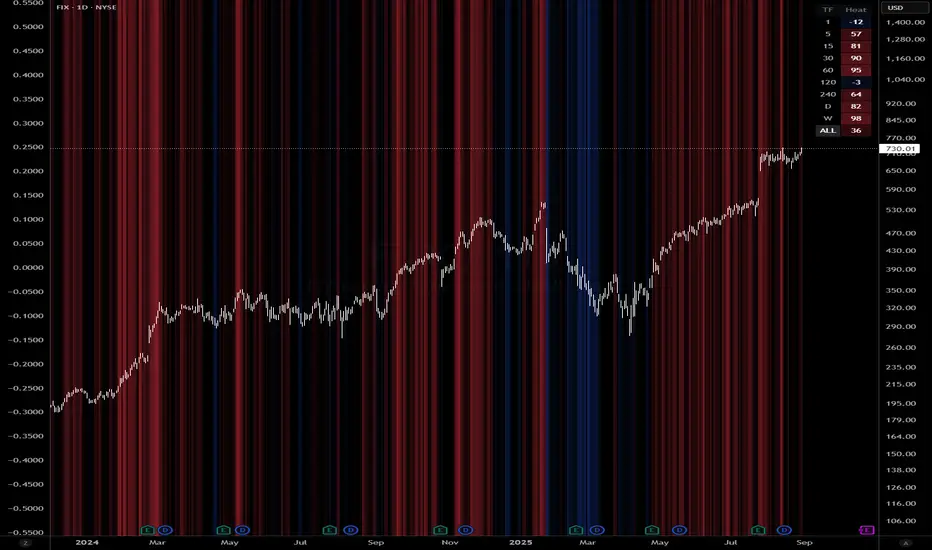
Harmonic Rolling VWAP (Zeiierman)█ Overview
The Harmonic Rolling VWAP (Zeiierman) indicator combines the concept of the Rolling Volume Weighted Average Price (VWAP) with advanced harmonic analysis using Discrete Fourier Transform (DFT). This innovative indicator aims to provide traders with a dynamic view of price action, capturing both the volume-weighted price and underlying harmonic patterns. By leveraging this combination, traders can gain deeper insights into market trends and potential reversal points.
█ How It Works
The Harmonic Rolling VWAP calculates the rolling VWAP over a specified window of bars, giving more weight to periods with higher trading volume. This VWAP is then subjected to harmonic analysis using the Discrete Fourier Transform (DFT), which decomposes the VWAP into its frequency components.
Key Components:
Rolling VWAP (RVWAP): A moving average that gives more weight to higher volume periods, calculated over a user-defined window.
True Range (TR): Measures volatility by comparing the current high and low prices, considering the previous close price.
Discrete Fourier Transform (DFT): Analyzes the harmonic patterns within the RVWAP by decomposing it into its frequency components.
Standard Deviation Bands: These bands provide a visual representation of price volatility around the RVWAP, helping traders identify potential overbought or oversold conditions.
█ How to Use
Identify Trends: The RVWAP line helps in identifying the underlying trend by smoothing out short-term price fluctuations and focusing on volume-weighted prices.
Assess Volatility: The standard deviation bands around the RVWAP give a clear view of price volatility, helping traders identify potential breakout or breakdown points.
Find Entry and Exit Points: Traders can look for entries when the price is near the lower bands in an uptrend or near the upper bands in a downtrend. Exits can be considered when the price approaches the opposite bands or shows harmonic divergence.
█ Settings
VWAP Source: Defines the price data used for VWAP calculations. The source input defines the price data used for calculations. This setting affects the VWAP calculations and the resulting bands.
Window: Sets the number of bars used for the rolling calculations. The window input sets the number of bars used for the rolling calculations. A larger window smooths the VWAP and standard deviation bands, making the indicator less sensitive to short-term price fluctuations. A smaller window makes the indicator more responsive to recent price changes.
-----------------
Disclaimer
The information contained in my Scripts/Indicators/Ideas/Algos/Systems does not constitute financial advice or a solicitation to buy or sell any securities of any type. I will not accept liability for any loss or damage, including without limitation any loss of profit, which may arise directly or indirectly from the use of or reliance on such information.
All investments involve risk, and the past performance of a security, industry, sector, market, financial product, trading strategy, backtest, or individual's trading does not guarantee future results or returns. Investors are fully responsible for any investment decisions they make. Such decisions should be based solely on an evaluation of their financial circumstances, investment objectives, risk tolerance, and liquidity needs.
My Scripts/Indicators/Ideas/Algos/Systems are only for educational purposes!

Nick_OS RangesUNDERSTANDING THE SCRIPT:
TIMEFRAME RESOLUTION:
* You have the option to choose Daily , Weekly , or Monthly
LOOKBACK WINDOW:
* This number represents how far back you want the data to pull from
- Example: "250" would represent the past 250 Days, Weeks, or Months depending on what is selected in the Timeframe Resolution
RANGE 1 nth (Gray lines):
* This number represents the range of the nth biggest day, week, or month in the Lookback Window
- Example: "30" would represent the range of the 30th biggest day in the past 250 days. (If the Lookback Window is "250")
RANGE 2 nth (Blue lines):
* This number represents the range of the nth biggest day, week, or month in the Lookback Window
- Example: "10" would represent the range of the 10th biggest day in the past 250 days. (If the Lookback Window is "250")
RANGE 3 nth (Pink lines):
* This number represents the range of the nth biggest day, week, or month in the Lookback Window
- Example: "3" would represent the range of the 3rd biggest day in the past 250 days. (If the Lookback Window is "250")
YELLOW LINES:
* The yellow lines are the average percentage move of the inputted number in the Lookback Window
SUGGESTED INPUTS:
FOR DAILY:
Lookback Window: 250
Range 1 nth: 30
Range 2 nth: 10
Range 3 nth: 3
FOR WEEKLY:
Lookback Window: 50
Range 1 nth: 10
Range 2 nth: 5
Range 3 nth: 2
FOR MONTHLY:
Lookback Window: 12
Range 1 nth: 3
Range 2 nth: 2
Range 3 nth: 1
TIMEFRAMES TO USE (If You Have TradingView Premium):
Daily: 5 minute timeframe and higher (15 minute timeframe and higher for Futures)
Weekly: 15 minute timeframe and higher
Monthly: Daily timeframe and higher (Monthly still has issues)
TIMEFRAMES TO USE (If You DO NOT Have TradingView Premium):
Daily: 15 minute timeframe and higher
Weekly: 30 minute timeframe and higher
Monthly: Daily timeframe and higher (Monthly still has issues)
IMPORTANT RELATED NOTE:
If you decide to use a higher Lookback Window, the ranges might be off and the timeframes listed above might not apply
ISSUES THAT MIGHT BE RESOLVED IN THE FUTURE
1. If it is a shortened week (No Monday or Friday), then the Weekly Ranges will show the same ranges as last week
2. Monthly ranges will change based on any timeframe used

Variety, Low-Pass, FIR Filter Impulse Response Explorer [Loxx]Variety Low-Pass FIR Filter, Impulse Response Explorer is a simple impulse response explorer of 16 of the most popular FIR digital filtering windowing techniques. Y-values are the values of the coefficients produced by the selected algorithms; X-values are the index of sample. This indicator also allows you to turn on Sinc Windowing for all window types except for Rectangular, Triangular, and Linear. This is an educational indicator to demonstrate the differences between popular FIR filters in terms of their coefficient outputs. This is also used to compliment other indicators I've published or will publish that implement advanced FIR digital filters (see below to find applicable indicators).
Inputs:
Number of Coefficients to Calculate = Sample size; for example, this would be the period used in SMA or WMA
FIR Digital Filter Type = FIR windowing method you would like to explore
Multiplier (Sinc only) = applies a multiplier effect to the Sinc Windowing
Frequency Cutoff = this is necessary to smooth the output and get rid of noise. the lower the number, the smoother the output.
Turn on Sinc? = turn this on if you want to convert the windowing function from regular function to a Windowed-Sinc filter
Order = This is used for power of cosine filter only. This is the N-order, or depth, of the filter you wish to create.
What are FIR Filters?
In discrete-time signal processing, windowing is a preliminary signal shaping technique, usually applied to improve the appearance and usefulness of a subsequent Discrete Fourier Transform. Several window functions can be defined, based on a constant (rectangular window), B-splines, other polynomials, sinusoids, cosine-sums, adjustable, hybrid, and other types. The windowing operation consists of multipying the given sampled signal by the window function. For trading purposes, these FIR filters act as advanced weighted moving averages.
A finite impulse response (FIR) filter is a filter whose impulse response (or response to any finite length input) is of finite duration, because it settles to zero in finite time. This is in contrast to infinite impulse response (IIR) filters, which may have internal feedback and may continue to respond indefinitely (usually decaying).
The impulse response (that is, the output in response to a Kronecker delta input) of an Nth-order discrete-time FIR filter lasts exactly {\displaystyle N+1}N+1 samples (from first nonzero element through last nonzero element) before it then settles to zero.
FIR filters can be discrete-time or continuous-time, and digital or analog.
A FIR filter is (similar to, or) just a weighted moving average filter, where (unlike a typical equally weighted moving average filter) the weights of each delay tap are not constrained to be identical or even of the same sign. By changing various values in the array of weights (the impulse response, or time shifted and sampled version of the same), the frequency response of a FIR filter can be completely changed.
An FIR filter simply CONVOLVES the input time series (price data) with its IMPULSE RESPONSE. The impulse response is just a set of weights (or "coefficients") that multiply each data point. Then you just add up all the products and divide by the sum of the weights and that is it; e.g., for a 10-bar SMA you just add up 10 bars of price data (each multiplied by 1) and divide by 10. For a weighted-MA you add up the product of the price data with triangular-number weights and divide by the total weight.
What's a Low-Pass Filter?
A low-pass filter is the type of frequency domain filter that is used for smoothing sound, image, or data. This is different from a high-pass filter that is used for sharpening data, images, or sound.
Whats a Windowed-Sinc Filter?
Windowed-sinc filters are used to separate one band of frequencies from another. They are very stable, produce few surprises, and can be pushed to incredible performance levels. These exceptional frequency domain characteristics are obtained at the expense of poor performance in the time domain, including excessive ripple and overshoot in the step response. When carried out by standard convolution, windowed-sinc filters are easy to program, but slow to execute.
The sinc function sinc (x), also called the "sampling function," is a function that arises frequently in signal processing and the theory of Fourier transforms.
In mathematics, the historical unnormalized sinc function is defined for x ≠ 0 by
sinc x = sinx / x
In digital signal processing and information theory, the normalized sinc function is commonly defined for x ≠ 0 by
sinc x = sin(pi * x) / (pi * x)
For our purposes here, we are used a normalized Sinc function
Included Windowing Functions
N-Order Power-of-Cosine (this one is really N-different types of FIR filters)
Hamming
Hanning
Blackman
Blackman Harris
Blackman Nutall
Nutall
Bartlet Zero End Points
Bartlet-Hann
Hann
Sine
Lanczos
Flat Top
Rectangular
Linear
Triangular
If you wish to dive deeper to get a full explanation of these windowing functions, see here: en.wikipedia.org
Related indicators
STD-Filtered, Variety FIR Digital Filters w/ ATR Bands
STD/C-Filtered, N-Order Power-of-Cosine FIR Filter
STD/C-Filtered, Truncated Taylor Family FIR Filter
STD/Clutter-Filtered, Kaiser Window FIR Digital Filter
STD/Clutter Filtered, One-Sided, N-Sinc-Kernel, EFIR Filt
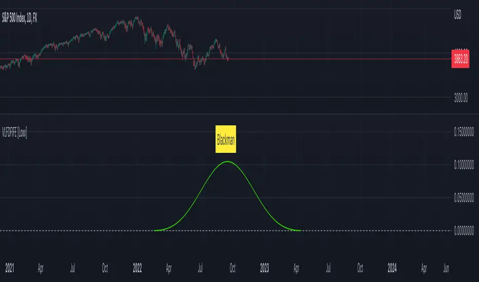
DR/IDR fractals break candle (ChadAnt)This indicator is an Opening Range Breakout (ORB) tool. It identifies the high and low price range established during a specific time window (e.g., the first hour of trading, 9:30–10:30 AM NY time). Once that time window closes, it watches for the price to "break out" of that range and projects profit targets based on the size of the initial range.
Key Features & How They Work
1. The Opening Range (The Box)
Time Window: The indicator waits for your specific start time (default 9:30 AM NY). It does not draw anything before this time.
The "Wicks": It tracks the absolute highest and lowest prices reached during this time (the Wicks). These act as your Breakout Triggers.
The "Body": It tracks the highest and lowest candle closes/opens during this time. This creates a shaded "zone" on your chart, representing the core area where most trading occurred.
Shading: To keep your chart clean, the background shading only appears during the forming time window.
2. Breakout Signals
Once the time window ends (e.g., 10:30 AM), the indicator "locks" the levels.
It then waits for a candle to move above the Wick High or below the Wick Low.
The Signal: When this happens, a label ("BREAK") appears on the chart.
Green Label: Bullish breakout (price went above the range).
Red Label: Bearish breakout (price went below the range).
Note: It only signals the first breakout of the day to avoid false alarms during choppy markets.
3. Extension Targets (Profit Levels)
When a breakout signal occurs, the indicator automatically draws target lines (extensions).
Calculation: These targets are based on the height of the "Body" zone (the shaded area).
Example: If your setting is 1.0, the indicator measures the height of the shaded body range and projects that exact distance above the breakout point. This is often used as a "Measured Move" target.
You can customize how many lines appear and how far apart they are (e.g., 0.5, 1.0, 1.5 times the range size).
4. Williams Fractals
During the opening range time, the indicator looks for specific price patterns called "Williams Fractals" (a 5-candle pattern that highlights potential turning points).
If a fractal peak or valley occurs inside your opening range, it marks it with a small triangle (▲ or ▼). Traders often use these as early signs of support or resistance forming inside the range.
5. Clean Visuals
Line Cutoff: You can set a "Stop Time" (e.g., 16:00 or 4:00 PM). The lines will stop drawing at that time so they don't clutter your chart overnight.
Gap Handling: The lines are programmed to break cleanly between days, so you don't see messy diagonal lines connecting yesterday's close to today's open.
Summary of Settings You Can Change
Session Time: When the range starts and ends.
Line Stop Time: When the lines should disappear for the day.
Visuals: Colors, line width, and style (solid, dotted, dashed).
Extensions: How many target lines to draw and the step size (e.g., 0.5x, 1.0x).
Fractals: Toggle the triangle icons on/off.

ALN Sessions Box — Auto- DSTDevoleper: Sheikh Rakib
What it does
Draws candle-synced high/low range boxes for the three major sessions—Asia (Dhaka view), London, and New York—on any timeframe. London and New York are DST-aware (times auto-shift on DST changes). Boxes update live with session high/low and close exactly on the session’s final bar.
Key features
Auto-DST: Uses Europe/London and America/New_York time zones, so session windows auto-adjust when DST turns on/off.
Asia (BDT) window: Default 06:00–15:00 Asia/Dhaka (no DST).
Candle-linked boxes: Top/bottom track session High/Low; right edge finalizes on the session end bar—clean breakout zones.
Clean UI: Optional labels, outline toggle, and three opacity presets (Dark/Medium/Light).
Plug & play: Drop in, customize colors/times, done.
Inputs you can tweak
Time Range (LOCAL) for each session
Defaults: Asia 06:00–15:00 (Asia/Dhaka), London 08:00–17:00 (Europe/London), New York 08:00–17:00 (America/New_York)
For equities, switch New York to 09:30–16:00—DST handling remains automatic.
Colour per session, Show Session Labels, Show Range Outline, Opacity Preset.
UTC Offset input is retained for compatibility but not used for session detection.
Quick BDT reference (for the default 08:00–17:00 local windows)
London → DST ON (BST): 13:00–22:00 BDT · DST OFF (GMT): 14:00–23:00 BDT
New York → DST ON (EDT): 18:00–03:00 BDT (next day) · DST OFF (EST): 19:00–04:00 BDT (next day)
Asia (Dhaka) → 06:00–15:00 BDT (no DST)
Tips
If you see dotted vertical lines, that’s TradingView Session breaks (Chart Settings → Appearance). Turn off if you prefer a cleaner view.
Some symbols don’t trade during parts of a session—adjust Time Range as needed.
Labels are placed inside the box; adjust opacity/colors to suit your theme.
A sharp, professional session map for spotting breakouts, reversals, and volatility windows at a glance.
Quantum Rotational Field MappingQuantum Rotational Field Mapping (QRFM):
Phase Coherence Detection Through Complex-Plane Oscillator Analysis
Quantum Rotational Field Mapping applies complex-plane mathematics and phase-space analysis to oscillator ensembles, identifying high-probability trend ignition points by measuring when multiple independent oscillators achieve phase coherence. Unlike traditional multi-oscillator approaches that simply stack indicators or use boolean AND/OR logic, this system converts each oscillator into a rotating phasor (vector) in the complex plane and calculates the Coherence Index (CI) —a mathematical measure of how tightly aligned the ensemble has become—then generates signals only when alignment, phase direction, and pairwise entanglement all converge.
The indicator combines three mathematical frameworks: phasor representation using analytic signal theory to extract phase and amplitude from each oscillator, coherence measurement using vector summation in the complex plane to quantify group alignment, and entanglement analysis that calculates pairwise phase agreement across all oscillator combinations. This creates a multi-dimensional confirmation system that distinguishes between random oscillator noise and genuine regime transitions.
What Makes This Original
Complex-Plane Phasor Framework
This indicator implements classical signal processing mathematics adapted for market oscillators. Each oscillator—whether RSI, MACD, Stochastic, CCI, Williams %R, MFI, ROC, or TSI—is first normalized to a common scale, then converted into a complex-plane representation using an in-phase (I) and quadrature (Q) component. The in-phase component is the oscillator value itself, while the quadrature component is calculated as the first difference (derivative proxy), creating a velocity-aware representation.
From these components, the system extracts:
Phase (φ) : Calculated as φ = atan2(Q, I), representing the oscillator's position in its cycle (mapped to -180° to +180°)
Amplitude (A) : Calculated as A = √(I² + Q²), representing the oscillator's strength or conviction
This mathematical approach is fundamentally different from simply reading oscillator values. A phasor captures both where an oscillator is in its cycle (phase angle) and how strongly it's expressing that position (amplitude). Two oscillators can have the same value but be in opposite phases of their cycles—traditional analysis would see them as identical, while QRFM sees them as 180° out of phase (contradictory).
Coherence Index Calculation
The core innovation is the Coherence Index (CI) , borrowed from physics and signal processing. When you have N oscillators, each with phase φₙ, you can represent each as a unit vector in the complex plane: e^(iφₙ) = cos(φₙ) + i·sin(φₙ).
The CI measures what happens when you sum all these vectors:
Resultant Vector : R = Σ e^(iφₙ) = Σ cos(φₙ) + i·Σ sin(φₙ)
Coherence Index : CI = |R| / N
Where |R| is the magnitude of the resultant vector and N is the number of active oscillators.
The CI ranges from 0 to 1:
CI = 1.0 : Perfect coherence—all oscillators have identical phase angles, vectors point in the same direction, creating maximum constructive interference
CI = 0.0 : Complete decoherence—oscillators are randomly distributed around the circle, vectors cancel out through destructive interference
0 < CI < 1 : Partial alignment—some clustering with some scatter
This is not a simple average or correlation. The CI captures phase synchronization across the entire ensemble simultaneously. When oscillators phase-lock (align their cycles), the CI spikes regardless of their individual values. This makes it sensitive to regime transitions that traditional indicators miss.
Dominant Phase and Direction Detection
Beyond measuring alignment strength, the system calculates the dominant phase of the ensemble—the direction the resultant vector points:
Dominant Phase : φ_dom = atan2(Σ sin(φₙ), Σ cos(φₙ))
This gives the "average direction" of all oscillator phases, mapped to -180° to +180°:
+90° to -90° (right half-plane): Bullish phase dominance
+90° to +180° or -90° to -180° (left half-plane): Bearish phase dominance
The combination of CI magnitude (coherence strength) and dominant phase angle (directional bias) creates a two-dimensional signal space. High CI alone is insufficient—you need high CI plus dominant phase pointing in a tradeable direction. This dual requirement is what separates QRFM from simple oscillator averaging.
Entanglement Matrix and Pairwise Coherence
While the CI measures global alignment, the entanglement matrix measures local pairwise relationships. For every pair of oscillators (i, j), the system calculates:
E(i,j) = |cos(φᵢ - φⱼ)|
This represents the phase agreement between oscillators i and j:
E = 1.0 : Oscillators are in-phase (0° or 360° apart)
E = 0.0 : Oscillators are in quadrature (90° apart, orthogonal)
E between 0 and 1 : Varying degrees of alignment
The system counts how many oscillator pairs exceed a user-defined entanglement threshold (e.g., 0.7). This entangled pairs count serves as a confirmation filter: signals require not just high global CI, but also a minimum number of strong pairwise agreements. This prevents false ignitions where CI is high but driven by only two oscillators while the rest remain scattered.
The entanglement matrix creates an N×N symmetric matrix that can be visualized as a web—when many cells are bright (high E values), the ensemble is highly interconnected. When cells are dark, oscillators are moving independently.
Phase-Lock Tolerance Mechanism
A complementary confirmation layer is the phase-lock detector . This calculates the maximum phase spread across all oscillators:
For all pairs (i,j), compute angular distance: Δφ = |φᵢ - φⱼ|, wrapping at 180°
Max Spread = maximum Δφ across all pairs
If max spread < user threshold (e.g., 35°), the ensemble is considered phase-locked —all oscillators are within a narrow angular band.
This differs from entanglement: entanglement measures pairwise cosine similarity (magnitude of alignment), while phase-lock measures maximum angular deviation (tightness of clustering). Both must be satisfied for the highest-conviction signals.
Multi-Layer Visual Architecture
QRFM includes six visual components that represent the same underlying mathematics from different perspectives:
Circular Orbit Plot : A polar coordinate grid showing each oscillator as a vector from origin to perimeter. Angle = phase, radius = amplitude. This is a real-time snapshot of the complex plane. When vectors converge (point in similar directions), coherence is high. When scattered randomly, coherence is low. Users can see phase alignment forming before CI numerically confirms it.
Phase-Time Heat Map : A 2D matrix with rows = oscillators and columns = time bins. Each cell is colored by the oscillator's phase at that time (using a gradient where color hue maps to angle). Horizontal color bands indicate sustained phase alignment over time. Vertical color bands show moments when all oscillators shared the same phase (ignition points). This provides historical pattern recognition.
Entanglement Web Matrix : An N×N grid showing E(i,j) for all pairs. Cells are colored by entanglement strength—bright yellow/gold for high E, dark gray for low E. This reveals which oscillators are driving coherence and which are lagging. For example, if RSI and MACD show high E but Stochastic shows low E with everything, Stochastic is the outlier.
Quantum Field Cloud : A background color overlay on the price chart. Color (green = bullish, red = bearish) is determined by dominant phase. Opacity is determined by CI—high CI creates dense, opaque cloud; low CI creates faint, nearly invisible cloud. This gives an atmospheric "feel" for regime strength without looking at numbers.
Phase Spiral : A smoothed plot of dominant phase over recent history, displayed as a curve that wraps around price. When the spiral is tight and rotating steadily, the ensemble is in coherent rotation (trending). When the spiral is loose or erratic, coherence is breaking down.
Dashboard : A table showing real-time metrics: CI (as percentage), dominant phase (in degrees with directional arrow), field strength (CI × average amplitude), entangled pairs count, phase-lock status (locked/unlocked), quantum state classification ("Ignition", "Coherent", "Collapse", "Chaos"), and collapse risk (recent CI change normalized to 0-100%).
Each component is independently toggleable, allowing users to customize their workspace. The orbit plot is the most essential—it provides intuitive, visual feedback on phase alignment that no numerical dashboard can match.
Core Components and How They Work Together
1. Oscillator Normalization Engine
The foundation is creating a common measurement scale. QRFM supports eight oscillators:
RSI : Normalized from to using overbought/oversold levels (70, 30) as anchors
MACD Histogram : Normalized by dividing by rolling standard deviation, then clamped to
Stochastic %K : Normalized from using (80, 20) anchors
CCI : Divided by 200 (typical extreme level), clamped to
Williams %R : Normalized from using (-20, -80) anchors
MFI : Normalized from using (80, 20) anchors
ROC : Divided by 10, clamped to
TSI : Divided by 50, clamped to
Each oscillator can be individually enabled/disabled. Only active oscillators contribute to phase calculations. The normalization removes scale differences—a reading of +0.8 means "strongly bullish" regardless of whether it came from RSI or TSI.
2. Analytic Signal Construction
For each active oscillator at each bar, the system constructs the analytic signal:
In-Phase (I) : The normalized oscillator value itself
Quadrature (Q) : The bar-to-bar change in the normalized value (first derivative approximation)
This creates a 2D representation: (I, Q). The phase is extracted as:
φ = atan2(Q, I) × (180 / π)
This maps the oscillator to a point on the unit circle. An oscillator at the same value but rising (positive Q) will have a different phase than one that is falling (negative Q). This velocity-awareness is critical—it distinguishes between "at resistance and stalling" versus "at resistance and breaking through."
The amplitude is extracted as:
A = √(I² + Q²)
This represents the distance from origin in the (I, Q) plane. High amplitude means the oscillator is far from neutral (strong conviction). Low amplitude means it's near zero (weak/transitional state).
3. Coherence Calculation Pipeline
For each bar (or every Nth bar if phase sample rate > 1 for performance):
Step 1 : Extract phase φₙ for each of the N active oscillators
Step 2 : Compute complex exponentials: Zₙ = e^(i·φₙ·π/180) = cos(φₙ·π/180) + i·sin(φₙ·π/180)
Step 3 : Sum the complex exponentials: R = Σ Zₙ = (Σ cos φₙ) + i·(Σ sin φₙ)
Step 4 : Calculate magnitude: |R| = √
Step 5 : Normalize by count: CI_raw = |R| / N
Step 6 : Smooth the CI: CI = SMA(CI_raw, smoothing_window)
The smoothing step (default 2 bars) removes single-bar noise spikes while preserving structural coherence changes. Users can adjust this to control reactivity versus stability.
The dominant phase is calculated as:
φ_dom = atan2(Σ sin φₙ, Σ cos φₙ) × (180 / π)
This is the angle of the resultant vector R in the complex plane.
4. Entanglement Matrix Construction
For all unique pairs of oscillators (i, j) where i < j:
Step 1 : Get phases φᵢ and φⱼ
Step 2 : Compute phase difference: Δφ = φᵢ - φⱼ (in radians)
Step 3 : Calculate entanglement: E(i,j) = |cos(Δφ)|
Step 4 : Store in symmetric matrix: matrix = matrix = E(i,j)
The matrix is then scanned: count how many E(i,j) values exceed the user-defined threshold (default 0.7). This count is the entangled pairs metric.
For visualization, the matrix is rendered as an N×N table where cell brightness maps to E(i,j) intensity.
5. Phase-Lock Detection
Step 1 : For all unique pairs (i, j), compute angular distance: Δφ = |φᵢ - φⱼ|
Step 2 : Wrap angles: if Δφ > 180°, set Δφ = 360° - Δφ
Step 3 : Find maximum: max_spread = max(Δφ) across all pairs
Step 4 : Compare to tolerance: phase_locked = (max_spread < tolerance)
If phase_locked is true, all oscillators are within the specified angular cone (e.g., 35°). This is a boolean confirmation filter.
6. Signal Generation Logic
Signals are generated through multi-layer confirmation:
Long Ignition Signal :
CI crosses above ignition threshold (e.g., 0.80)
AND dominant phase is in bullish range (-90° < φ_dom < +90°)
AND phase_locked = true
AND entangled_pairs >= minimum threshold (e.g., 4)
Short Ignition Signal :
CI crosses above ignition threshold
AND dominant phase is in bearish range (φ_dom < -90° OR φ_dom > +90°)
AND phase_locked = true
AND entangled_pairs >= minimum threshold
Collapse Signal :
CI at bar minus CI at current bar > collapse threshold (e.g., 0.55)
AND CI at bar was above 0.6 (must collapse from coherent state, not from already-low state)
These are strict conditions. A high CI alone does not generate a signal—dominant phase must align with direction, oscillators must be phase-locked, and sufficient pairwise entanglement must exist. This multi-factor gating dramatically reduces false signals compared to single-condition triggers.
Calculation Methodology
Phase 1: Oscillator Computation and Normalization
On each bar, the system calculates the raw values for all enabled oscillators using standard Pine Script functions:
RSI: ta.rsi(close, length)
MACD: ta.macd() returning histogram component
Stochastic: ta.stoch() smoothed with ta.sma()
CCI: ta.cci(close, length)
Williams %R: ta.wpr(length)
MFI: ta.mfi(hlc3, length)
ROC: ta.roc(close, length)
TSI: ta.tsi(close, short, long)
Each raw value is then passed through a normalization function:
normalize(value, overbought_level, oversold_level) = 2 × (value - oversold) / (overbought - oversold) - 1
This maps the oscillator's typical range to , where -1 represents extreme bearish, 0 represents neutral, and +1 represents extreme bullish.
For oscillators without fixed ranges (MACD, ROC, TSI), statistical normalization is used: divide by a rolling standard deviation or fixed divisor, then clamp to .
Phase 2: Phasor Extraction
For each normalized oscillator value val:
I = val (in-phase component)
Q = val - val (quadrature component, first difference)
Phase calculation:
phi_rad = atan2(Q, I)
phi_deg = phi_rad × (180 / π)
Amplitude calculation:
A = √(I² + Q²)
These values are stored in arrays: osc_phases and osc_amps for each oscillator n.
Phase 3: Complex Summation and Coherence
Initialize accumulators:
sum_cos = 0
sum_sin = 0
For each oscillator n = 0 to N-1:
phi_rad = osc_phases × (π / 180)
sum_cos += cos(phi_rad)
sum_sin += sin(phi_rad)
Resultant magnitude:
resultant_mag = √(sum_cos² + sum_sin²)
Coherence Index (raw):
CI_raw = resultant_mag / N
Smoothed CI:
CI = SMA(CI_raw, smoothing_window)
Dominant phase:
phi_dom_rad = atan2(sum_sin, sum_cos)
phi_dom_deg = phi_dom_rad × (180 / π)
Phase 4: Entanglement Matrix Population
For i = 0 to N-2:
For j = i+1 to N-1:
phi_i = osc_phases × (π / 180)
phi_j = osc_phases × (π / 180)
delta_phi = phi_i - phi_j
E = |cos(delta_phi)|
matrix_index_ij = i × N + j
matrix_index_ji = j × N + i
entangle_matrix = E
entangle_matrix = E
if E >= threshold:
entangled_pairs += 1
The matrix uses flat array storage with index mapping: index(row, col) = row × N + col.
Phase 5: Phase-Lock Check
max_spread = 0
For i = 0 to N-2:
For j = i+1 to N-1:
delta = |osc_phases - osc_phases |
if delta > 180:
delta = 360 - delta
max_spread = max(max_spread, delta)
phase_locked = (max_spread < tolerance)
Phase 6: Signal Evaluation
Ignition Long :
ignition_long = (CI crosses above threshold) AND
(phi_dom > -90 AND phi_dom < 90) AND
phase_locked AND
(entangled_pairs >= minimum)
Ignition Short :
ignition_short = (CI crosses above threshold) AND
(phi_dom < -90 OR phi_dom > 90) AND
phase_locked AND
(entangled_pairs >= minimum)
Collapse :
CI_prev = CI
collapse = (CI_prev - CI > collapse_threshold) AND (CI_prev > 0.6)
All signals are evaluated on bar close. The crossover and crossunder functions ensure signals fire only once when conditions transition from false to true.
Phase 7: Field Strength and Visualization Metrics
Average Amplitude :
avg_amp = (Σ osc_amps ) / N
Field Strength :
field_strength = CI × avg_amp
Collapse Risk (for dashboard):
collapse_risk = (CI - CI) / max(CI , 0.1)
collapse_risk_pct = clamp(collapse_risk × 100, 0, 100)
Quantum State Classification :
if (CI > threshold AND phase_locked):
state = "Ignition"
else if (CI > 0.6):
state = "Coherent"
else if (collapse):
state = "Collapse"
else:
state = "Chaos"
Phase 8: Visual Rendering
Orbit Plot : For each oscillator, convert polar (phase, amplitude) to Cartesian (x, y) for grid placement:
radius = amplitude × grid_center × 0.8
x = radius × cos(phase × π/180)
y = radius × sin(phase × π/180)
col = center + x (mapped to grid coordinates)
row = center - y
Heat Map : For each oscillator row and time column, retrieve historical phase value at lookback = (columns - col) × sample_rate, then map phase to color using a hue gradient.
Entanglement Web : Render matrix as table cell with background color opacity = E(i,j).
Field Cloud : Background color = (phi_dom > -90 AND phi_dom < 90) ? green : red, with opacity = mix(min_opacity, max_opacity, CI).
All visual components render only on the last bar (barstate.islast) to minimize computational overhead.
How to Use This Indicator
Step 1 : Apply QRFM to your chart. It works on all timeframes and asset classes, though 15-minute to 4-hour timeframes provide the best balance of responsiveness and noise reduction.
Step 2 : Enable the dashboard (default: top right) and the circular orbit plot (default: middle left). These are your primary visual feedback tools.
Step 3 : Optionally enable the heat map, entanglement web, and field cloud based on your preference. New users may find all visuals overwhelming; start with dashboard + orbit plot.
Step 4 : Observe for 50-100 bars to let the indicator establish baseline coherence patterns. Markets have different "normal" CI ranges—some instruments naturally run higher or lower coherence.
Understanding the Circular Orbit Plot
The orbit plot is a polar grid showing oscillator vectors in real-time:
Center point : Neutral (zero phase and amplitude)
Each vector : A line from center to a point on the grid
Vector angle : The oscillator's phase (0° = right/east, 90° = up/north, 180° = left/west, -90° = down/south)
Vector length : The oscillator's amplitude (short = weak signal, long = strong signal)
Vector label : First letter of oscillator name (R = RSI, M = MACD, etc.)
What to watch :
Convergence : When all vectors cluster in one quadrant or sector, CI is rising and coherence is forming. This is your pre-signal warning.
Scatter : When vectors point in random directions (360° spread), CI is low and the market is in a non-trending or transitional regime.
Rotation : When the cluster rotates smoothly around the circle, the ensemble is in coherent oscillation—typically seen during steady trends.
Sudden flips : When the cluster rapidly jumps from one side to the opposite (e.g., +90° to -90°), a phase reversal has occurred—often coinciding with trend reversals.
Example: If you see RSI, MACD, and Stochastic all pointing toward 45° (northeast) with long vectors, while CCI, TSI, and ROC point toward 40-50° as well, coherence is high and dominant phase is bullish. Expect an ignition signal if CI crosses threshold.
Reading Dashboard Metrics
The dashboard provides numerical confirmation of what the orbit plot shows visually:
CI : Displays as 0-100%. Above 70% = high coherence (strong regime), 40-70% = moderate, below 40% = low (poor conditions for trend entries).
Dom Phase : Angle in degrees with directional arrow. ⬆ = bullish bias, ⬇ = bearish bias, ⬌ = neutral.
Field Strength : CI weighted by amplitude. High values (> 0.6) indicate not just alignment but strong alignment.
Entangled Pairs : Count of oscillator pairs with E > threshold. Higher = more confirmation. If minimum is set to 4, you need at least 4 pairs entangled for signals.
Phase Lock : 🔒 YES (all oscillators within tolerance) or 🔓 NO (spread too wide).
State : Real-time classification:
🚀 IGNITION: CI just crossed threshold with phase-lock
⚡ COHERENT: CI is high and stable
💥 COLLAPSE: CI has dropped sharply
🌀 CHAOS: Low CI, scattered phases
Collapse Risk : 0-100% scale based on recent CI change. Above 50% warns of imminent breakdown.
Interpreting Signals
Long Ignition (Blue Triangle Below Price) :
Occurs when CI crosses above threshold (e.g., 0.80)
Dominant phase is in bullish range (-90° to +90°)
All oscillators are phase-locked (within tolerance)
Minimum entangled pairs requirement met
Interpretation : The oscillator ensemble has transitioned from disorder to coherent bullish alignment. This is a high-probability long entry point. The multi-layer confirmation (CI + phase direction + lock + entanglement) ensures this is not a single-oscillator whipsaw.
Short Ignition (Red Triangle Above Price) :
Same conditions as long, but dominant phase is in bearish range (< -90° or > +90°)
Interpretation : Coherent bearish alignment has formed. High-probability short entry.
Collapse (Circles Above and Below Price) :
CI has dropped by more than the collapse threshold (e.g., 0.55) over a 5-bar window
CI was previously above 0.6 (collapsing from coherent state)
Interpretation : Phase coherence has broken down. If you are in a position, this is an exit warning. If looking to enter, stand aside—regime is transitioning.
Phase-Time Heat Map Patterns
Enable the heat map and position it at bottom right. The rows represent individual oscillators, columns represent time bins (most recent on left).
Pattern: Horizontal Color Bands
If a row (e.g., RSI) shows consistent color across columns (say, green for several bins), that oscillator has maintained stable phase over time. If all rows show horizontal bands of similar color, the entire ensemble has been phase-locked for an extended period—this is a strong trending regime.
Pattern: Vertical Color Bands
If a column (single time bin) shows all cells with the same or very similar color, that moment in time had high coherence. These vertical bands often align with ignition signals or major price pivots.
Pattern: Rainbow Chaos
If cells are random colors (red, green, yellow mixed with no pattern), coherence is low. The ensemble is scattered. Avoid trading during these periods unless you have external confirmation.
Pattern: Color Transition
If you see a row transition from red to green (or vice versa) sharply, that oscillator has phase-flipped. If multiple rows do this simultaneously, a regime change is underway.
Entanglement Web Analysis
Enable the web matrix (default: opposite corner from heat map). It shows an N×N grid where N = number of active oscillators.
Bright Yellow/Gold Cells : High pairwise entanglement. For example, if the RSI-MACD cell is bright gold, those two oscillators are moving in phase. If the RSI-Stochastic cell is bright, they are entangled as well.
Dark Gray Cells : Low entanglement. Oscillators are decorrelated or in quadrature.
Diagonal : Always marked with "—" because an oscillator is always perfectly entangled with itself.
How to use :
Scan for clustering: If most cells are bright, coherence is high across the board. If only a few cells are bright, coherence is driven by a subset (e.g., RSI and MACD are aligned, but nothing else is—weak signal).
Identify laggards: If one row/column is entirely dark, that oscillator is the outlier. You may choose to disable it or monitor for when it joins the group (late confirmation).
Watch for web formation: During low-coherence periods, the matrix is mostly dark. As coherence builds, cells begin lighting up. A sudden "web" of connections forming visually precedes ignition signals.
Trading Workflow
Step 1: Monitor Coherence Level
Check the dashboard CI metric or observe the orbit plot. If CI is below 40% and vectors are scattered, conditions are poor for trend entries. Wait.
Step 2: Detect Coherence Building
When CI begins rising (say, from 30% to 50-60%) and you notice vectors on the orbit plot starting to cluster, coherence is forming. This is your alert phase—do not enter yet, but prepare.
Step 3: Confirm Phase Direction
Check the dominant phase angle and the orbit plot quadrant where clustering is occurring:
Clustering in right half (0° to ±90°): Bullish bias forming
Clustering in left half (±90° to 180°): Bearish bias forming
Verify the dashboard shows the corresponding directional arrow (⬆ or ⬇).
Step 4: Wait for Signal Confirmation
Do not enter based on rising CI alone. Wait for the full ignition signal:
CI crosses above threshold
Phase-lock indicator shows 🔒 YES
Entangled pairs count >= minimum
Directional triangle appears on chart
This ensures all layers have aligned.
Step 5: Execute Entry
Long : Blue triangle below price appears → enter long
Short : Red triangle above price appears → enter short
Step 6: Position Management
Initial Stop : Place stop loss based on your risk management rules (e.g., recent swing low/high, ATR-based buffer).
Monitoring :
Watch the field cloud density. If it remains opaque and colored in your direction, the regime is intact.
Check dashboard collapse risk. If it rises above 50%, prepare for exit.
Monitor the orbit plot. If vectors begin scattering or the cluster flips to the opposite side, coherence is breaking.
Exit Triggers :
Collapse signal fires (circles appear)
Dominant phase flips to opposite half-plane
CI drops below 40% (coherence lost)
Price hits your profit target or trailing stop
Step 7: Post-Exit Analysis
After exiting, observe whether a new ignition forms in the opposite direction (reversal) or if CI remains low (transition to range). Use this to decide whether to re-enter, reverse, or stand aside.
Best Practices
Use Price Structure as Context
QRFM identifies when coherence forms but does not specify where price will go. Combine ignition signals with support/resistance levels, trendlines, or chart patterns. For example:
Long ignition near a major support level after a pullback: high-probability bounce
Long ignition in the middle of a range with no structure: lower probability
Multi-Timeframe Confirmation
Open QRFM on two timeframes simultaneously:
Higher timeframe (e.g., 4-hour): Use CI level to determine regime bias. If 4H CI is above 60% and dominant phase is bullish, the market is in a bullish regime.
Lower timeframe (e.g., 15-minute): Execute entries on ignition signals that align with the higher timeframe bias.
This prevents counter-trend trades and increases win rate.
Distinguish Between Regime Types
High CI, stable dominant phase (State: Coherent) : Trending market. Ignitions are continuation signals; collapses are profit-taking or reversal warnings.
Low CI, erratic dominant phase (State: Chaos) : Ranging or choppy market. Avoid ignition signals or reduce position size. Wait for coherence to establish.
Moderate CI with frequent collapses : Whipsaw environment. Use wider stops or stand aside.
Adjust Parameters to Instrument and Timeframe
Crypto/Forex (high volatility) : Lower ignition threshold (0.65-0.75), lower CI smoothing (2-3), shorter oscillator lengths (7-10).
Stocks/Indices (moderate volatility) : Standard settings (threshold 0.75-0.85, smoothing 5-7, oscillator lengths 14).
Lower timeframes (5-15 min) : Reduce phase sample rate to 1-2 for responsiveness.
Higher timeframes (daily+) : Increase CI smoothing and oscillator lengths for noise reduction.
Use Entanglement Count as Conviction Filter
The minimum entangled pairs setting controls signal strictness:
Low (1-2) : More signals, lower quality (acceptable if you have other confirmation)
Medium (3-5) : Balanced (recommended for most traders)
High (6+) : Very strict, fewer signals, highest quality
Adjust based on your trade frequency preference and risk tolerance.
Monitor Oscillator Contribution
Use the entanglement web to see which oscillators are driving coherence. If certain oscillators are consistently dark (low E with all others), they may be adding noise. Consider disabling them. For example:
On low-volume instruments, MFI may be unreliable → disable MFI
On strongly trending instruments, mean-reversion oscillators (Stochastic, RSI) may lag → reduce weight or disable
Respect the Collapse Signal
Collapse events are early warnings. Price may continue in the original direction for several bars after collapse fires, but the underlying regime has weakened. Best practice:
If in profit: Take partial or full profit on collapse
If at breakeven/small loss: Exit immediately
If collapse occurs shortly after entry: Likely a false ignition; exit to avoid drawdown
Collapses do not guarantee immediate reversals—they signal uncertainty .
Combine with Volume Analysis
If your instrument has reliable volume:
Ignitions with expanding volume: Higher conviction
Ignitions with declining volume: Weaker, possibly false
Collapses with volume spikes: Strong reversal signal
Collapses with low volume: May just be consolidation
Volume is not built into QRFM (except via MFI), so add it as external confirmation.
Observe the Phase Spiral
The spiral provides a quick visual cue for rotation consistency:
Tight, smooth spiral : Ensemble is rotating coherently (trending)
Loose, erratic spiral : Phase is jumping around (ranging or transitional)
If the spiral tightens, coherence is building. If it loosens, coherence is dissolving.
Do Not Overtrade Low-Coherence Periods
When CI is persistently below 40% and the state is "Chaos," the market is not in a regime where phase analysis is predictive. During these times:
Reduce position size
Widen stops
Wait for coherence to return
QRFM's strength is regime detection. If there is no regime, the tool correctly signals "stand aside."
Use Alerts Strategically
Set alerts for:
Long Ignition
Short Ignition
Collapse
Phase Lock (optional)
Configure alerts to "Once per bar close" to avoid intrabar repainting and noise. When an alert fires, manually verify:
Orbit plot shows clustering
Dashboard confirms all conditions
Price structure supports the trade
Do not blindly trade alerts—use them as prompts for analysis.
Ideal Market Conditions
Best Performance
Instruments :
Liquid, actively traded markets (major forex pairs, large-cap stocks, major indices, top-tier crypto)
Instruments with clear cyclical oscillator behavior (avoid extremely illiquid or manipulated markets)
Timeframes :
15-minute to 4-hour: Optimal balance of noise reduction and responsiveness
1-hour to daily: Slower, higher-conviction signals; good for swing trading
5-minute: Acceptable for scalping if parameters are tightened and you accept more noise
Market Regimes :
Trending markets with periodic retracements (where oscillators cycle through phases predictably)
Breakout environments (coherence forms before/during breakout; collapse occurs at exhaustion)
Rotational markets with clear swings (oscillators phase-lock at turning points)
Volatility :
Moderate to high volatility (oscillators have room to move through their ranges)
Stable volatility regimes (sudden VIX spikes or flash crashes may create false collapses)
Challenging Conditions
Instruments :
Very low liquidity markets (erratic price action creates unstable oscillator phases)
Heavily news-driven instruments (fundamentals may override technical coherence)
Highly correlated instruments (oscillators may all reflect the same underlying factor, reducing independence)
Market Regimes :
Deep, prolonged consolidation (oscillators remain near neutral, CI is chronically low, few signals fire)
Extreme chop with no directional bias (oscillators whipsaw, coherence never establishes)
Gap-driven markets (large overnight gaps create phase discontinuities)
Timeframes :
Sub-5-minute charts: Noise dominates; oscillators flip rapidly; coherence is fleeting and unreliable
Weekly/monthly: Oscillators move extremely slowly; signals are rare; better suited for long-term positioning than active trading
Special Cases :
During major economic releases or earnings: Oscillators may lag price or become decorrelated as fundamentals overwhelm technicals. Reduce position size or stand aside.
In extremely low-volatility environments (e.g., holiday periods): Oscillators compress to neutral, CI may be artificially high due to lack of movement, but signals lack follow-through.
Adaptive Behavior
QRFM is designed to self-adapt to poor conditions:
When coherence is genuinely absent, CI remains low and signals do not fire
When only a subset of oscillators aligns, entangled pairs count stays below threshold and signals are filtered out
When phase-lock cannot be achieved (oscillators too scattered), the lock filter prevents signals
This means the indicator will naturally produce fewer (or zero) signals during unfavorable conditions, rather than generating false signals. This is a feature —it keeps you out of low-probability trades.
Parameter Optimization by Trading Style
Scalping (5-15 Minute Charts)
Goal : Maximum responsiveness, accept higher noise
Oscillator Lengths :
RSI: 7-10
MACD: 8/17/6
Stochastic: 8-10, smooth 2-3
CCI: 14-16
Others: 8-12
Coherence Settings :
CI Smoothing Window: 2-3 bars (fast reaction)
Phase Sample Rate: 1 (every bar)
Ignition Threshold: 0.65-0.75 (lower for more signals)
Collapse Threshold: 0.40-0.50 (earlier exit warnings)
Confirmation :
Phase Lock Tolerance: 40-50° (looser, easier to achieve)
Min Entangled Pairs: 2-3 (fewer oscillators required)
Visuals :
Orbit Plot + Dashboard only (reduce screen clutter for fast decisions)
Disable heavy visuals (heat map, web) for performance
Alerts :
Enable all ignition and collapse alerts
Set to "Once per bar close"
Day Trading (15-Minute to 1-Hour Charts)
Goal : Balance between responsiveness and reliability
Oscillator Lengths :
RSI: 14 (standard)
MACD: 12/26/9 (standard)
Stochastic: 14, smooth 3
CCI: 20
Others: 10-14
Coherence Settings :
CI Smoothing Window: 3-5 bars (balanced)
Phase Sample Rate: 2-3
Ignition Threshold: 0.75-0.85 (moderate selectivity)
Collapse Threshold: 0.50-0.55 (balanced exit timing)
Confirmation :
Phase Lock Tolerance: 30-40° (moderate tightness)
Min Entangled Pairs: 4-5 (reasonable confirmation)
Visuals :
Orbit Plot + Dashboard + Heat Map or Web (choose one)
Field Cloud for regime backdrop
Alerts :
Ignition and collapse alerts
Optional phase-lock alert for advance warning
Swing Trading (4-Hour to Daily Charts)
Goal : High-conviction signals, minimal noise, fewer trades
Oscillator Lengths :
RSI: 14-21
MACD: 12/26/9 or 19/39/9 (longer variant)
Stochastic: 14-21, smooth 3-5
CCI: 20-30
Others: 14-20
Coherence Settings :
CI Smoothing Window: 5-10 bars (very smooth)
Phase Sample Rate: 3-5
Ignition Threshold: 0.80-0.90 (high bar for entry)
Collapse Threshold: 0.55-0.65 (only significant breakdowns)
Confirmation :
Phase Lock Tolerance: 20-30° (tight clustering required)
Min Entangled Pairs: 5-7 (strong confirmation)
Visuals :
All modules enabled (you have time to analyze)
Heat Map for multi-bar pattern recognition
Web for deep confirmation analysis
Alerts :
Ignition and collapse
Review manually before entering (no rush)
Position/Long-Term Trading (Daily to Weekly Charts)
Goal : Rare, very high-conviction regime shifts
Oscillator Lengths :
RSI: 21-30
MACD: 19/39/9 or 26/52/12
Stochastic: 21, smooth 5
CCI: 30-50
Others: 20-30
Coherence Settings :
CI Smoothing Window: 10-14 bars
Phase Sample Rate: 5 (every 5th bar to reduce computation)
Ignition Threshold: 0.85-0.95 (only extreme alignment)
Collapse Threshold: 0.60-0.70 (major regime breaks only)
Confirmation :
Phase Lock Tolerance: 15-25° (very tight)
Min Entangled Pairs: 6+ (broad consensus required)
Visuals :
Dashboard + Orbit Plot for quick checks
Heat Map to study historical coherence patterns
Web to verify deep entanglement
Alerts :
Ignition only (collapses are less critical on long timeframes)
Manual review with fundamental analysis overlay
Performance Optimization (Low-End Systems)
If you experience lag or slow rendering:
Reduce Visual Load :
Orbit Grid Size: 8-10 (instead of 12+)
Heat Map Time Bins: 5-8 (instead of 10+)
Disable Web Matrix entirely if not needed
Disable Field Cloud and Phase Spiral
Reduce Calculation Frequency :
Phase Sample Rate: 5-10 (calculate every 5-10 bars)
Max History Depth: 100-200 (instead of 500+)
Disable Unused Oscillators :
If you only want RSI, MACD, and Stochastic, disable the other five. Fewer oscillators = smaller matrices, faster loops.
Simplify Dashboard :
Choose "Small" dashboard size
Reduce number of metrics displayed
These settings will not significantly degrade signal quality (signals are based on bar-close calculations, which remain accurate), but will improve chart responsiveness.
Important Disclaimers
This indicator is a technical analysis tool designed to identify periods of phase coherence across an ensemble of oscillators. It is not a standalone trading system and does not guarantee profitable trades. The Coherence Index, dominant phase, and entanglement metrics are mathematical calculations applied to historical price data—they measure past oscillator behavior and do not predict future price movements with certainty.
No Predictive Guarantee : High coherence indicates that oscillators are currently aligned, which historically has coincided with trending or directional price movement. However, past alignment does not guarantee future trends. Markets can remain coherent while prices consolidate, or lose coherence suddenly due to news, liquidity changes, or other factors not captured by oscillator mathematics.
Signal Confirmation is Probabilistic : The multi-layer confirmation system (CI threshold + dominant phase + phase-lock + entanglement) is designed to filter out low-probability setups. This increases the proportion of valid signals relative to false signals, but does not eliminate false signals entirely. Users should combine QRFM with additional analysis—support and resistance levels, volume confirmation, multi-timeframe alignment, and fundamental context—before executing trades.
Collapse Signals are Warnings, Not Reversals : A coherence collapse indicates that the oscillator ensemble has lost alignment. This often precedes trend exhaustion or reversals, but can also occur during healthy pullbacks or consolidations. Price may continue in the original direction after a collapse. Use collapses as risk management cues (tighten stops, take partial profits) rather than automatic reversal entries.
Market Regime Dependency : QRFM performs best in markets where oscillators exhibit cyclical, mean-reverting behavior and where trends are punctuated by retracements. In markets dominated by fundamental shocks, gap openings, or extreme low-liquidity conditions, oscillator coherence may be less reliable. During such periods, reduce position size or stand aside.
Risk Management is Essential : All trading involves risk of loss. Use appropriate stop losses, position sizing, and risk-per-trade limits. The indicator does not specify stop loss or take profit levels—these must be determined by the user based on their risk tolerance and account size. Never risk more than you can afford to lose.
Parameter Sensitivity : The indicator's behavior changes with input parameters. Aggressive settings (low thresholds, loose tolerances) produce more signals with lower average quality. Conservative settings (high thresholds, tight tolerances) produce fewer signals with higher average quality. Users should backtest and forward-test parameter sets on their specific instruments and timeframes before committing real capital.
No Repainting by Design : All signal conditions are evaluated on bar close using bar-close values. However, the visual components (orbit plot, heat map, dashboard) update in real-time during bar formation for monitoring purposes. For trade execution, rely on the confirmed signals (triangles and circles) that appear only after the bar closes.
Computational Load : QRFM performs extensive calculations, including nested loops for entanglement matrices and real-time table rendering. On lower-powered devices or when running multiple indicators simultaneously, users may experience lag. Use the performance optimization settings (reduce visual complexity, increase phase sample rate, disable unused oscillators) to improve responsiveness.
This system is most effective when used as one component within a broader trading methodology that includes sound risk management, multi-timeframe analysis, market context awareness, and disciplined execution. It is a tool for regime detection and signal confirmation, not a substitute for comprehensive trade planning.
Technical Notes
Calculation Timing : All signal logic (ignition, collapse) is evaluated using bar-close values. The barstate.isconfirmed or implicit bar-close behavior ensures signals do not repaint. Visual components (tables, plots) render on every tick for real-time feedback but do not affect signal generation.
Phase Wrapping : Phase angles are calculated in the range -180° to +180° using atan2. Angular distance calculations account for wrapping (e.g., the distance between +170° and -170° is 20°, not 340°). This ensures phase-lock detection works correctly across the ±180° boundary.
Array Management : The indicator uses fixed-size arrays for oscillator phases, amplitudes, and the entanglement matrix. The maximum number of oscillators is 8. If fewer oscillators are enabled, array sizes shrink accordingly (only active oscillators are processed).
Matrix Indexing : The entanglement matrix is stored as a flat array with size N×N, where N is the number of active oscillators. Index mapping: index(row, col) = row × N + col. Symmetric pairs (i,j) and (j,i) are stored identically.
Normalization Stability : Oscillators are normalized to using fixed reference levels (e.g., RSI overbought/oversold at 70/30). For unbounded oscillators (MACD, ROC, TSI), statistical normalization (division by rolling standard deviation) is used, with clamping to prevent extreme outliers from distorting phase calculations.
Smoothing and Lag : The CI smoothing window (SMA) introduces lag proportional to the window size. This is intentional—it filters out single-bar noise spikes in coherence. Users requiring faster reaction can reduce the smoothing window to 1-2 bars, at the cost of increased sensitivity to noise.
Complex Number Representation : Pine Script does not have native complex number types. Complex arithmetic is implemented using separate real and imaginary accumulators (sum_cos, sum_sin) and manual calculation of magnitude (sqrt(real² + imag²)) and argument (atan2(imag, real)).
Lookback Limits : The indicator respects Pine Script's maximum lookback constraints. Historical phase and amplitude values are accessed using the operator, with lookback limited to the chart's available bar history (max_bars_back=5000 declared).
Visual Rendering Performance : Tables (orbit plot, heat map, web, dashboard) are conditionally deleted and recreated on each update using table.delete() and table.new(). This prevents memory leaks but incurs redraw overhead. Rendering is restricted to barstate.islast (last bar) to minimize computational load—historical bars do not render visuals.
Alert Condition Triggers : alertcondition() functions evaluate on bar close when their boolean conditions transition from false to true. Alerts do not fire repeatedly while a condition remains true (e.g., CI stays above threshold for 10 bars fires only once on the initial cross).
Color Gradient Functions : The phaseColor() function maps phase angles to RGB hues using sine waves offset by 120° (red, green, blue channels). This creates a continuous spectrum where -180° to +180° spans the full color wheel. The amplitudeColor() function maps amplitude to grayscale intensity. The coherenceColor() function uses cos(phase) to map contribution to CI (positive = green, negative = red).
No External Data Requests : QRFM operates entirely on the chart's symbol and timeframe. It does not use request.security() or access external data sources. All calculations are self-contained, avoiding lookahead bias from higher-timeframe requests.
Deterministic Behavior : Given identical input parameters and price data, QRFM produces identical outputs. There are no random elements, probabilistic sampling, or time-of-day dependencies.
— Dskyz, Engineering precision. Trading coherence.
