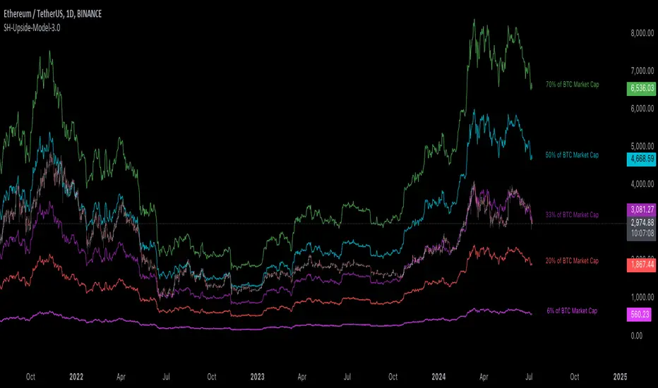
[Suitable Hope] Crypto Upside Model 3.0The "Crypto Upside Model 3.0" indicator dynamically calculates the potential price of any cryptocurrency based on various percentages of Ethereum or Bitcoin's market capitalization.
By fetching and analyzing marketcap data from TradingView sources, it allows traders to visualize potential price targets if their chosen cryptocurrency reaches specific market dominance levels. This tool is designed for daily timeframe analysis and can be used to set informed price expectations and strategic investment goals, providing valuable insights for long-term investment planning.
Why using the Crypto Upside Model 3.0?
Strategic Planning: Helps traders and investors set realistic price targets and investment goals by visualizing potential market cap scenarios.
Informed Decision-Making: Provides a data-driven approach to understanding how a cryptocurrency might perform relative to major assets like Bitcoin and Ethereum.
Customizable Analysis: Allows users to choose different comparison assets (ETH or BTC) and visualize various market cap dominance percentages, offering tailored insights.
Daily Timeframe Focus: Ideal for swing traders and long-term investors who operate on a daily analysis timeframe, providing relevant and actionable data.
Bull Markets: Identify potential price targets if your cryptocurrency's market cap increases significantly.
Bear Markets: Assess how much value could be retained relative to major cryptocurrencies.
Strategic Entry/Exit Points: Use the visualized targets to plan entry or exit points in your trading strategy.
Comparative Advantage
Dynamic Adaptation: Unlike fixed indicators, this tool adapts to any active chart, making it versatile for multiple cryptocurrencies.
Market Cap Insights: Provides a unique perspective by linking price targets to market cap dominance, a critical factor in the crypto market.
User Instructions
Setup: Add the " Upside Model 3.0" indicator to your TradingView chart.
Configuration: Use the input settings to select the comparison cryptocurrency (ETH or BTC) and enable the desired market cap percentage plots.
Analysis: The indicator will display potential price targets based on the selected market cap percentages, providing a visual guide for setting price expectations.
Limitations
Marketcap Data Availability: The indicator relies on marketcap data from TradingView, which may not be available for all cryptocurrencies. If the data is unavailable, the indicator will not function for that asset. This tool is more likely to work with older, established cryptocurrencies, as marketcap data for newer cryptocurrencies may not yet be available.
Daily Timeframe Restriction: The indicator is designed to work exclusively on the daily timeframe, limiting its applicability for intraday trading.
Assumptions of Market Dynamics: The calculations assume a direct correlation between market dominance and price, which may not account for other market dynamics and external factors influencing prices.
Data Accuracy: The accuracy of the indicator depends on the reliability of the data provided by TradingView, which may sometimes experience delays or inaccuracies.
Currently available cryptocurrencies: Bitcoin, Ethereum, Solana, Binance Coin, Cardano, Ripple, Polkadot, Avalanche, Chainlink, Litecoin, Dogecoin, Terra, Uniswap, VeChain, Stellar, Internet Computer, Hedera, Filecoin, Monero, Aave, TRON, NEAR Protocol, Compound, Maker,... For all compatible cryptocurrencies, please consult CRYPTOCAP's documentation.
Final notes
Although various sources ask a payment or user data for similar kind of private indicators, this one is entirely free and open source. "Uncanny" isn't it? I hope this indicator will provide you value. Feel free to leave a message if you have any questions or constructive feedback.
Examples of how I use this indicator
When using ETH's historical price as a reference compared to Bitcoin's marketcap, we can notice that price generally has been held between the +-30% and 50% lines of BTC's marketcap. If history is repeating again, we can expect major resistances around the 50% looking ahead into the future. This for me would be a great area to potentially reduce my ETH spot position.
When using SOL's historical price action, we can notice that the 15% line of ETH's marketcap has been a top in the previous cycle. Today SOL (July 2024), is back at this level. Could this be a top again or could price break this 15% level and head perhaps towards 30% which currently sits around $260? Time will tell.
These are 2 simple example of how I interpret the data. I'm keen to hear what other findings with other pairs you can find.
Cerca negli script per "安泰科技+2024年6月+股价走势"
[Pandora] Vast Volatility Treasure TroveINTRODUCTION:
Volatility enthusiasts, prepare for VICTORY on this day of July 4th, 2024! This is my "Vast Volatility Treasure Trove," intended mostly for educational purposes, yet these functions will also exhibit versatility when combined with other algorithms to garner statistical excellence. Once again, I am now ripping the lid off of Pandora's box... of volatility. Inside this script is a 'vast' collection of volatility estimators, reflecting the indicators name. Whether you are a seasoned trader destined to navigate financial strife or an eagerly curious learner, this script offers a comprehensive toolkit for a broad spectrum of volatility analysis. Enjoy your journey through the realm of market volatility with this code!
WHAT IS MARKET VOLATILITY?:
Market volatility refers to various fluctuations in the value of a financial market or asset over a period of time, often characterized by occasional rapid and significant deviations in price. During periods of greater market volatility, evolving conditions of prices can move rapidly in either direction, creating uncertainty for investors with results of sharp declines as well as rapid gains. However, market volatility is a typical aspect expected in financial markets that can also present opportunities for informed decision-making and potential benefits from the price flux.
SCRIPT INTENTION:
Volatility is assuredly omnipresent, waxing and waning in magnitude, and some readers have every intention of studying and/or measuring it. This script serves as an all-in-one armada of volatility estimators for TradingView members. I set out to provide a diverse set of tools to analyze and interpret market volatility, offering volatile insights, and aid with the development of robust trading indicators and strategies.
In today's fast-paced financial markets, understanding and quantifying volatility is informative for both seasoned traders and novice investors. This script is designed to empower users by equipping them with a comprehensive suite of volatility estimators. Each function within this script has been meticulously crafted to address various aspects of volatility, from traditional methods like Garman-Klass and Parkinson to more advanced techniques like Yang-Zhang and my custom experimental algorithms.
Ultimately, this script is more than just a collection of functions. It is a gateway to a deeper understanding of market volatility and a valuable resource for anyone committed to mastering the complexities of financial markets.
SCRIPT CONTENTS:
This script includes a variety of functions designed to measure and analyze market volatility. Where applicable, an input checkbox option provides an unbiased/biased estimate. Below is a brief description of each function in the original order they appear as code upon first publish:
Parkinson Volatility - Estimates volatility emphasizing the high and low range movements.
Alternate Parkinson Volatility - Simpler version of the original Parkinson Volatility that I realized.
Garman-Klass Volatility - Estimates volatility based on high, low, open, and close prices using a formula that adjusts for biases in price dynamics.
Rogers-Satchell-Yoon Volatility #1 - Estimates volatility based on logarithmic differences between high, low, open, and close values.
Rogers-Satchell-Yoon Volatility #2 - Similar estimate to Rogers-Satchell with the same result via an alternate formulation of volatility.
Yang-Zhang Volatility - An advanced volatility estimate combining both strengths of the Garman-Klass and Rogers-Satchell estimators, with weights determined by an alpha parameter.
Yang-Zhang (Modified) Volatility - My experimental modification slightly different from the Yang-Zhang formula with improved computational efficiency.
Selectable Volatility - Basic customizable volatility calculation based on the logarithmic difference between selected numerator and denominator prices (e.g., open, high, low, close).
Close-to-Close Volatility - Estimates volatility using the logarithmic difference between consecutive closing prices. Specifically applicable to data sources without open, high, and low prices.
Open-to-Close Volatility - (Overnight Volatility): Estimates volatility based on the logarithmic difference between the opening price and the last closing price emphasizing overnight gaps.
Hilo Volatility - Estimates volatility using a method similar to Parkinson's method, which considers the logarithm of the high and low prices.
Vantage Volatility - My experimental custom 'vantage' method to estimate volatility similar to Yang-Zhang, which incorporates various factors (Alpha, Beta, Gamma) to generate a weighted logarithmic calculation. This may be a volatility advantage or disadvantage, hence it's name.
Schwert Volatility - Estimates volatility based on arithmetic returns.
Historical Volatility - Estimates volatility considering logarithmic returns.
Annualized Historical Volatility - Estimates annualized volatility using logarithmic returns, adjusted for the number of trading days in a year.
If I omitted any other known varieties, detailed requests for future consideration can be made below for their inclusion into this script within future versions...
BONUS ALGORITHMS:
This script also includes several experimental and bonus functions that push the boundaries of volatility analysis as I understand it. These functions are designed to provide additional insights and also are my ideal notions for traders looking to explore other methods of volatility measurement.
VOLATILITY APPLICATIONS:
Volatility estimators serve a common role across various facets of trading and financial analysis, offering insights into market behavior. These tools are already in instrumental with enhancing risk management practices by providing a deeper understanding of market dynamics and the inherent uncertainty in asset prices. With volatility estimators, traders can effectively quantifying market risk and adjust their strategies accordingly, optimizing portfolio performance and mitigating potential losses. Additionally, volatility estimations may serve as indication for detecting overbought or oversold market conditions, offering probabilistic insights that could inform strategic decisions at turning points. This script
distinctly offers a variety of volatility estimators to navigate intricate financial terrains with informed judgment to address challenges of strategic planning.
CODE REUSE:
You don't have to ask for my permission to use/reuse these functions in your published scripts, simply because I have better things to do than answer requests for the reuse of these functions.
Notice: Unfortunately, I will not provide any integration support into member's projects at all. I have my own projects that require way too much of my day already.

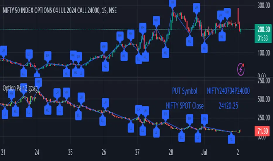
Option Pair ZigzagOptions Pair Zigzag:
Though we can split the chart window and view multiple charts, this indicator is useful when we view options charts.
How this indicator works:
The indicator works in non-overlay mode.
The indicator will find other option pair symbol and load it’s chart in indicator window. It will also draw a zigzag on both the charts. It will also fetch the SPOT symbol and display SPOT Close price of latest candle.
Useful information:
A. Support resistance: Higher High (HH) and Lower Low (LL) markings can be treated as strong support and or resistance and LH, HL markings can be treated as weak support and or resistance.
B. Trend identification: Easy identification of trend based on trend lines and trend markings i.e. Higher High (HH), Lower Low (LL), Lower High (LH), Higher Low (HL)
C. Use of Rate of change (ROC )– Labels drawn on swing points are equipped with ROC% between swing points. ROC% between Call and Put option charts can be compared and used to identify strong and weak moves.
Example:
1. User loads a call option chart of ‘NIFTY240620C23500’ (NIFTY 50 INDEX OPTIONS 20 JUN 2024 CALL 23500)
2. Since user has selected CALL Option, Indicator rules/logic will find PUT Option symbol of same strike and expiry
3. PUT Option chart would then shown in the indicator window
4. Draw zigzag on both the charts
5. Plot labels on both the charts
6. Labels are equipped with a tooltip showing rate of change between 2 pivot points
Input Parameters:
Left bars – Parameter required for plotting zigzag
Right bars – Parameter required for plotting zigzag
Plot HHLL Labels – Enable/disable plotting of labels
Use cases:
Refer to chart snapshots:
1. Buy Call Option or Sell Put Option - How one can trade on formation of a consolidation range
2. Breakdown of Swing structure - One can observe Swing structure (Zigzag) formed on a SPOT chart and trade on break of swing structure
3. Triangle formation - Observe the patterns formed on the SPOT chart and trade either Call or Put options. Example snapshot shows trade based on triangle pattern
Chart Snapshot:
One can split chart window and load base symbol chart which will help to review bases symbol and options chart at the same time.
Buy Call Option or Sell Put Option
Breakdown of Swing structure
Triangle formation
US Presidential Elections (Names & Dates)US Presidential Elections (Names & Dates)
Description :
This indicator marks key dates in US presidential history, highlighting both election days and inauguration dates. It's designed to provide historical context to your charts, allowing you to see how major political events align with market movements.
Key Features:
• Displays US presidential elections from 1936 to 2052
• Shows inauguration dates for each president
• Customizable colors and styles for both election and inauguration markers
• Toggle visibility of election and inauguration labels separately
• Adapts to different timeframes (daily, weekly, monthly)
• Includes president names for historical context
The indicator uses yellow labels for election days and blue labels for inauguration dates. Election labels show the year and "Election", while inauguration labels display the name of the incoming president.
Customization options include:
• Colors for election and inauguration labels and text
• Line widths for both types of events
• Label placement styles
This tool is perfect for traders and analysts who want to correlate political events with market trends over long periods. It provides a unique perspective on how presidential cycles might influence financial markets.
Note: Future elections (2024 onwards) are marked with a placeholder (✅) as the presidents are not yet known.
Use this indicator to:
• Identify potential market patterns around election cycles
• Analyze historical market reactions to specific presidencies
• Add political context to your long-term chart analysis
Enhance your chart analysis with this comprehensive view of US presidential history!

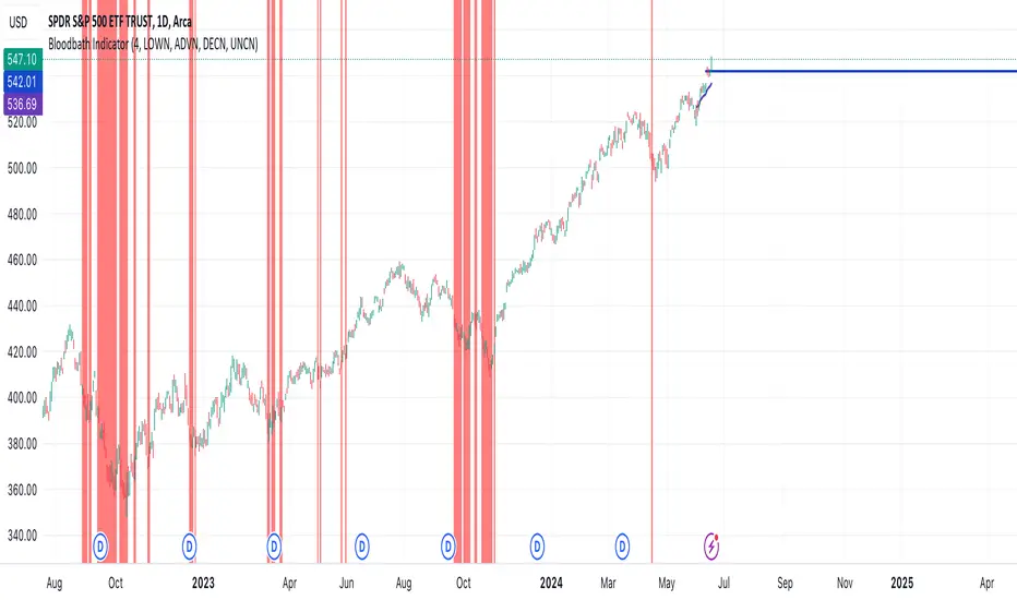
Bloodbath IndicatorThis indicator identifies days where the number of new 52-week lows for all issues exceeds a user-defined threshold (default 4%), potentially signaling a market downturn. The background of the chart turns red on such days, providing a visual alert to traders following the "Bloodbath Sidestepping" strategy.
Based on: "THE RIPPLE EFFECT OF DAILY NEW LOWS," By Ralph Vince and Larry Williams, 2024 Charles H. Dow Award Winner
threshold: Percentage of issues making new 52-week lows to trigger the indicator (default: 4.0).
Usage:
The chart background will turn red on days exceeding the threshold of new 52-week lows.
Limitations:
This indicator relies on historical data and doesn't guarantee future performance.
It focuses solely on new 52-week lows and may miss other market signals.
The strategy may generate false positives and requires further analysis before trading decisions.
Disclaimer:
This script is for informational purposes only and should not be considered financial advice. Always conduct your own research before making any trading decisions.
Sharpe and Sortino Ratios█ OVERVIEW
This indicator calculates the Sharpe and Sortino ratios using a chart symbol's periodic price returns, offering insights into the symbol's risk-adjusted performance. It features the option to calculate these ratios by comparing the periodic returns to a fixed annual rate of return or the returns from another selected symbol's context.
█ CONCEPTS
Returns, risk, and volatility
The return on an investment is the relative gain or loss over a period, often expressed as a percentage. Investment returns can originate from several sources, including capital gains, dividends, and interest income. Many investors seek the highest returns possible in the quest for profit. However, prudent investing and trading entails evaluating such returns against the associated risks (i.e., the uncertainty of returns and the potential for financial losses) for a clearer perspective on overall performance and sustainability.
The profitability of an investment typically comes at the cost of enduring market swings, noise, and general uncertainty. To navigate these turbulent waters, investors and portfolio managers often utilize volatility , a measure of the statistical dispersion of historical returns, as a foundational element in their risk assessments because it provides a tangible way to gauge the uncertainty in returns. High volatility suggests increased uncertainty and, consequently, higher risk, whereas low volatility suggests more stable returns with minimal fluctuations, implying lower risk. These concepts are integral components in several risk-adjusted performance metrics, including the Sharpe and Sortino ratios calculated by this indicator.
Risk-free rate
The risk-free rate represents the rate of return on a hypothetical investment carrying no risk of financial loss. This theoretical rate provides a benchmark for comparing the returns on a risky investment and evaluating whether its excess returns justify the risks. If an investment's returns are at or below the theoretical risk-free rate or the risk premium is below a desired amount, it may suggest that the returns do not compensate for the extra risk, which might be a call to reassess the investment.
Since the risk-free rate is a theoretical concept, investors often utilize proxies for the rate in practice, such as Treasury bills and other government bonds. Conventionally, analysts consider such instruments "risk-free" for a domestic holder, as they are a form of government obligation with a low perceived likelihood of default.
The average yield on short-term Treasury bills, influenced by economic conditions, monetary policies, and inflation expectations, has historically hovered around 2-3% over the long term. This range also aligns with central banks' inflation targets. As such, one may interpret a value within this range as a minimum proxy for the risk-free rate, as it may correspond to the minimum rate required to maintain purchasing power over time. This indicator uses a default value of 2% as the risk-free rate in its Sharpe and Sortino ratio calculations. Users can adjust this value from the "Risk-free rate of return" input in the "Settings/Inputs" tab.
Sharpe and Sortino ratios
The Sharpe and Sortino ratios are two of the most widely used metrics that offer insight into an investment's risk-adjusted performance . They provide a standardized framework to compare the effectiveness of investments relative to their perceived risks. These metrics can help investors determine whether the returns justify the risks taken to achieve them, promoting more informed investment decisions.
Both metrics measure risk-adjusted performance similarly. However, they have some differences in their formulas and their interpretation:
1. Sharpe ratio
The Sharpe ratio , developed by Nobel laureate William F. Sharpe, measures the performance of an investment compared to a theoretically risk-free asset, adjusted for the investment risk. The ratio uses the following formula:
Sharpe Ratio = (𝑅𝑎 − 𝑅𝑓) / 𝜎𝑎
Where:
• 𝑅𝑎 = Average return of the investment
• 𝑅𝑓 = Theoretical risk-free rate of return
• 𝜎𝑎 = Standard deviation of the investment's returns (volatility)
A higher Sharpe ratio indicates a more favorable risk-adjusted return, as it signifies that the investment produced higher excess returns per unit of increase in total perceived risk.
2. Sortino ratio
The Sortino ratio is a modified form of the Sharpe ratio that only considers downside volatility , i.e., the volatility of returns below the theoretical risk-free benchmark. Although it shares close similarities with the Sharpe ratio, it can produce very different values, especially when the returns do not have a symmetrical distribution, since it does not penalize upside and downside volatility equally. The ratio uses the following formula:
Sortino Ratio = (𝑅𝑎 − 𝑅𝑓) / 𝜎𝑑
Where:
• 𝑅𝑎 = Average return of the investment
• 𝑅𝑓 = Theoretical risk-free rate of return
• 𝜎𝑑 = Downside deviation (standard deviation of negative excess returns, or downside volatility)
The Sortino ratio offers an alternative perspective on an investment's return-generating efficiency since it does not consider upside volatility in its calculation. A higher Sortino ratio signifies that the investment produced higher excess returns per unit of increase in perceived downside risk.
The risk-free rate (𝑅𝑓) in the numerator of both ratio formulas acts as a baseline for comparing an investment's performance to a theoretical risk-free alternative. By subtracting the risk-free rate from the expected return (𝑅𝑎−𝑅𝑓), the numerator essentially represents the risk premium of the investment.
Comparison with another symbol
In addition to the conventional Sharpe and Sortino ratios, which compare an instrument's returns to a risk-free rate, this indicator can also compare returns to a user-specified benchmark symbol , allowing the calculation of Information ratios .
An Information ratio is a generalized form of the Sharpe ratio that compares an investment's returns to a risky benchmark , such as SPY, rather than a risk-free rate. It measures the investment's active return (the difference between its returns and the benchmark returns) relative to its tracking error (i.e., the volatility of the active return) using the following formula:
𝐼𝑅 = (𝑅𝑝 − 𝑅𝑏) / 𝑇𝐸
Where:
• 𝑅𝑝 = Average return on the portfolio or investment
• 𝑅𝑏 = Average return from the benchmark instrument
• 𝑇𝐸 = Tracking error (volatility of 𝑅𝑝 − 𝑅𝑏)
Comparing returns to a benchmark instrument rather than a theoretical risk-free rate offers unique insights into risk-adjusted performance. Higher Information ratios signify that the investment produced higher active returns per unit of increase in risk relative to the benchmark. Conventional choices for non-risk-free benchmarks include major composite indices like the S&P 500 and DJIA, as the resulting ratios can provide insight into the effectiveness of an investment relative to the broader market.
Users can enable this generalized calculation for both the Sharpe and Sortino ratios by selecting the "Benchmark symbol returns" option from the "Benchmark type" dropdown in the "Settings/Inputs" tab.
It's crucial to note that this indicator compares the charts symbol's rate of change (return) to the rate of change in the benchmark symbol. Consequently, not all symbols available on TradingView are suitable for use with these ratios due to the nature of what their values represent. For instance, using a bond as a benchmark will produce distorted results since each bar's values represent yields rather than prices, meaning it compares the rate of change in the yield. To maintain consistency and relevance in the calculated ratios, ensure the values from the compared symbols strictly represent price information.
█ FEATURES
This indicator provides traders with two widely used metrics for assessing risk-adjusted performance, generalized to allow users to compare the chart symbol's price returns to a fixed risk-free rate or the returns from another risky symbol. Below are the key features of this indicator:
Timeframe selection
The "Returns timeframe" input determines the timeframe of the calculated price returns. Users can select any value greater than or equal to the chart's timeframe. The default timeframe is "1M".
Periodic returns tracking
This indicator compounds and collects requested price returns from the selected timeframe over monthly or daily periods, similar to how the Broker Emulator works when calculating strategy performance metrics on trade data. It employs the following logic:
• Track returns over monthly periods if the chart's data spans at least two months.
• Track returns over daily periods if the chart's data spans at least two days but not two months.
• Do not track or collect returns if the data spans less than two days, as the amount of data is insufficient for meaningful ratio calculations.
The indicator uses the returns collected from up to a specified number of periods to calculate the Sharpe and Sortino ratios, depending on the available historical data. It also uses these periodic returns to calculate the average returns it displays in the Data Window.
Users can control the maximum number of periods the indicator analyzes with the "Max no. of periods used" input in the "Settings/Inputs" tab. The default value is 60 periods.
Benchmark specification
The "Benchmark return type" input specifies the benchmark type the indicator compares to the chart symbol's returns in the ratio calculations. It features the following two options:
• "Risk-free rate of return (%)": Compares the price returns to a user-specified annual rate of return representing a theoretical risk-free rate (e.g., 2%).
• "Benchmark symbol return": Compares the price returns to a selected benchmark symbol (e.g., "AMEX:SPY) to calculate Information ratios.
When comparing a chart symbol's returns to a specified benchmark symbol, this indicator aligns the times of data points from the benchmark with the times of data points from the chart's symbol to facilitate a fair comparison between symbols with different active sessions.
Visualization and display
• The indicator displays the periodic returns requested from the specified "Returns timeframe" in a separate pane. The plot includes dynamic colors to signify positive and negative returns.
• When the "Returns timeframe" value represents a higher timeframe, the indicator displays background highlights on the main chart pane to signify when a new value is available and whether the return is positive or negative.
• When the specified benchmark return type is a benchmark symbol, the indicator displays the requested symbol's returns in the separate pane as a gray line for visual comparison.
• Within the separate pane, the indicator displays a single-cell table that shows the base period it uses for periodic returns, the number of periods it uses in the calculation, the timeframe of the requested data, and the calculated Sharpe and Sortino ratios.
• The Data Window displays the chart symbol and benchmark returns, their periodic averages, and the Sharpe and Sortino ratios.
█ FOR Pine Script™ CODERS
• This script utilizes the functions from our RiskMetrics library to determine the size of the periods, calculate and collect periodic returns, and compute the Sharpe and Sortino ratios.
• The `getAlignedPrices()` function in this script requests price data for the chart's symbol and a benchmark symbol with consistent time alignment by utilizing spread symbols , which helps facilitate a fair comparison between different symbol types. Retrieving prices from spreads avoids potential information loss and data misalignment that can otherwise occur when using separate requests from each symbol's context when those symbols have different sessions or data times.
• For consistency, the `getAlignedPrices()` function includes extended hours and dividend adjustment modifiers in its data requests. Additionally, it includes other settings inherited from the chart's context, such as "settlement-as-close" preferences for fair comparison between futures instruments.
• This script uses the `changePercent()` function from our ta library to calculate the percentage changes of the requested data.
• The newly released `force_overlay` parameter in display-related functions allows indicators to display visuals on the main chart and a separate pane simultaneously. We use the parameter in this script's bgcolor() call to display background highlights on the main chart.
Look first. Then leap.

Smart Money Analysis with Golden/Death Cross [YourTradingSensei]Description of the script "Smart Money Analysis with Golden/Death Cross":
This TradingView script is designed for market analysis based on the concept of "Smart Money" and includes the detection of Golden Cross and Death Cross signals.
Key features of the script:
Moving Averages (SMA):
Two moving averages are calculated: a short-term (50 periods) and a long-term (200 periods).
The intersections of these moving averages are used to determine Golden Cross and Death Cross signals.
High Volume:
The current trading volume is analyzed.
Periods of high volume are identified when the current volume exceeds the average volume by a specified multiplier.
Support and Resistance Levels:
Key support and resistance levels are determined based on the highest and lowest prices over a specified period.
Buy and Sell Signals:
Buy and sell signals are generated based on moving average crossovers, high volume, and the closing price relative to key levels.
Golden Cross and Death Cross:
A Golden Cross occurs when the short-term moving average crosses above the long-term moving average.
A Death Cross occurs when the short-term moving average crosses below the long-term moving average.
These signals are displayed on the chart with text color changes for better visualization.
Using the script:
The script helps traders visualize key signals and levels, aiding in making informed trading decisions based on the behavior of major market players and technical analysis.
Custom candle lighting(CCL) © 2024 by YourTradingSensei is licensed under CC BY-NC-SA 4.0. To view a copy of this license.

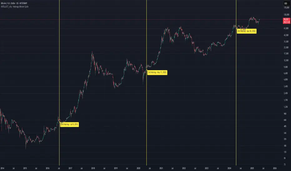
Intellect_city - Halvings Bitcoin CycleWhat is halving?
The halving timer shows when the next Bitcoin halving will occur, as well as the dates of past halvings. This event occurs every 210,000 blocks, which is approximately every 4 years. Halving reduces the emission reward by half. The original Bitcoin reward was 50 BTC per block found.
Why is halving necessary?
Halving allows you to maintain an algorithmically specified emission level. Anyone can verify that no more than 21 million bitcoins can be issued using this algorithm. Moreover, everyone can see how much was issued earlier, at what speed the emission is happening now, and how many bitcoins remain to be mined in the future. Even a sharp increase or decrease in mining capacity will not significantly affect this process. In this case, during the next difficulty recalculation, which occurs every 2014 blocks, the mining difficulty will be recalculated so that blocks are still found approximately once every ten minutes.
How does halving work in Bitcoin blocks?
The miner who collects the block adds a so-called coinbase transaction. This transaction has no entry, only exit with the receipt of emission coins to your address. If the miner's block wins, then the entire network will consider these coins to have been obtained through legitimate means. The maximum reward size is determined by the algorithm; the miner can specify the maximum reward size for the current period or less. If he puts the reward higher than possible, the network will reject such a block and the miner will not receive anything. After each halving, miners have to halve the reward they assign to themselves, otherwise their blocks will be rejected and will not make it to the main branch of the blockchain.
The impact of halving on the price of Bitcoin
It is believed that with constant demand, a halving of supply should double the value of the asset. In practice, the market knows when the halving will occur and prepares for this event in advance. Typically, the Bitcoin rate begins to rise about six months before the halving, and during the halving itself it does not change much. On average for past periods, the upper peak of the rate can be observed more than a year after the halving. It is almost impossible to predict future periods because, in addition to the reduction in emissions, many other factors influence the exchange rate. For example, major hacks or bankruptcies of crypto companies, the situation on the stock market, manipulation of “whales,” or changes in legislative regulation.
---------------------------------------------
Table - Past and future Bitcoin halvings:
---------------------------------------------
Date: Number of blocks: Award:
0 - 03-01-2009 - 0 block - 50 BTC
1 - 28-11-2012 - 210000 block - 25 BTC
2 - 09-07-2016 - 420000 block - 12.5 BTC
3 - 11-05-2020 - 630000 block - 6.25 BTC
4 - 20-04-2024 - 840000 block - 3.125 BTC
5 - 24-03-2028 - 1050000 block - 1.5625 BTC
6 - 26-02-2032 - 1260000 block - 0.78125 BTC
7 - 30-01-2036 - 1470000 block - 0.390625 BTC
8 - 03-01-2040 - 1680000 block - 0.1953125 BTC
9 - 07-12-2043 - 1890000 block - 0.09765625 BTC
10 - 10-11-2047 - 2100000 block - 0.04882813 BTC
11 - 14-10-2051 - 2310000 block - 0.02441406 BTC
12 - 17-09-2055 - 2520000 block - 0.01220703 BTC
13 - 21-08-2059 - 2730000 block - 0.00610352 BTC
14 - 25-07-2063 - 2940000 block - 0.00305176 BTC
15 - 28-06-2067 - 3150000 block - 0.00152588 BTC
16 - 01-06-2071 - 3360000 block - 0.00076294 BTC
17 - 05-05-2075 - 3570000 block - 0.00038147 BTC
18 - 08-04-2079 - 3780000 block - 0.00019073 BTC
19 - 12-03-2083 - 3990000 block - 0.00009537 BTC
20 - 13-02-2087 - 4200000 block - 0.00004768 BTC
21 - 17-01-2091 - 4410000 block - 0.00002384 BTC
22 - 21-12-2094 - 4620000 block - 0.00001192 BTC
23 - 24-11-2098 - 4830000 block - 0.00000596 BTC
24 - 29-10-2102 - 5040000 block - 0.00000298 BTC
25 - 02-10-2106 - 5250000 block - 0.00000149 BTC
26 - 05-09-2110 - 5460000 block - 0.00000075 BTC
27 - 09-08-2114 - 5670000 block - 0.00000037 BTC
28 - 13-07-2118 - 5880000 block - 0.00000019 BTC
29 - 16-06-2122 - 6090000 block - 0.00000009 BTC
30 - 20-05-2126 - 6300000 block - 0.00000005 BTC
31 - 23-04-2130 - 6510000 block - 0.00000002 BTC
32 - 27-03-2134 - 6720000 block - 0.00000001 BTC
MarkdownUtilsLibrary "MarkdownUtils"
This library shows all of CommonMark's formatting elements that are currently (2024-03-30)
available in Pine Script® and gives some hints on how to use them.
The documentation will be in the tooltip of each of the following functions. It is also
logged into Pine Logs by default if it is called. We can disable the logging by setting `pLog = false`.
mediumMathematicalSpace()
Medium mathematical space that can be used in e.g. the library names like `Markdown Utils`.
Returns: The medium mathematical space character U+205F between those double quotes " ".
zeroWidthSpace()
Zero-width space.
Returns: The zero-width character U+200B between those double quotes "".
stableSpace(pCount)
Consecutive space characters in Pine Script® are replaced by a single space character on output.
Therefore we require a "stable" space to properly indent text e.g. in Pine Logs. To use it in code blocks
of a description like this one, we have to copy the 2(!) characters between the following reverse brackets instead:
# > <
Those are the zero-width character U+200B and a space.
Of course, this can also be used within a text to add some extra spaces.
Parameters:
pCount (simple int)
Returns: A zero-width space combined with a space character.
headers(pLog)
Headers
```
# H1
## H2
### H3
#### H4
##### H5
###### H6
```
*results in*
# H1
## H2
### H3
#### H4
##### H5
###### H6
*Best practices*: Add blank line before and after each header.
Parameters:
pLog (bool)
paragrahps(pLog)
Paragraphs
```
First paragraph
Second paragraph
```
*results in*
First paragraph
Second paragraph
Parameters:
pLog (bool)
lineBreaks(pLog)
Line breaks
```
First row
Second row
```
*results in*
First row\
Second row
Parameters:
pLog (bool)
emphasis(pLog)
Emphasis
With surrounding `*` and `~` we can emphasize text as follows. All emphasis can be arbitrarily combined.
```
*Italics*, **Bold**, ***Bold italics***, ~~Scratch~~
```
*results in*
*Italics*, **Bold**, ***Bold italics***, ~~Scratch~~
Parameters:
pLog (bool)
blockquotes(pLog)
Blockquotes
Lines starting with at least one `>` followed by a space and text build block quotes.
```
Text before blockquotes.
> 1st main blockquote
>
> 1st main blockquote
>
>> 1st 1-nested blockquote
>
>>> 1st 2-nested blockquote
>
>>>> 1st 3-nested blockquote
>
>>>>> 1st 4-nested blockquote
>
>>>>>> 1st 5-nested blockquote
>
>>>>>>> 1st 6-nested blockquote
>
>>>>>>>> 1st 7-nested blockquote
>
> 2nd main blockquote, 1st paragraph, 1st row\
> 2nd main blockquote, 1st paragraph, 2nd row
>
> 2nd main blockquote, 2nd paragraph, 1st row\
> 2nd main blockquote, 2nd paragraph, 2nd row
>
>> 2nd nested blockquote, 1st paragraph, 1st row\
>> 2nd nested blockquote, 1st paragraph, 2nd row
>
>> 2nd nested blockquote, 2nd paragraph, 1st row\
>> 2nd nested blockquote, 2nd paragraph, 2nd row
Text after blockquotes.
```
*results in*
Text before blockquotes.
> 1st main blockquote
>
>> 1st 1-nested blockquote
>
>>> 1st 2-nested blockquote
>
>>>> 1st 3-nested blockquote
>
>>>>> 1st 4-nested blockquote
>
>>>>>> 1st 5-nested blockquote
>
>>>>>>> 1st 6-nested blockquote
>
>>>>>>>> 1st 7-nested blockquote
>
> 2nd main blockquote, 1st paragraph, 1st row\
> 2nd main blockquote, 1st paragraph, 2nd row
>
> 2nd main blockquote, 2nd paragraph, 1st row\
> 2nd main blockquote, 2nd paragraph, 2nd row
>
>> 2nd nested blockquote, 1st paragraph, 1st row\
>> 2nd nested blockquote, 1st paragraph, 2nd row
>
>> 2nd nested blockquote, 2nd paragraph, 1st row\
>> 2nd nested blockquote, 2nd paragraph, 2nd row
Text after blockquotes.
*Best practices*: Add blank line before and after each (nested) blockquote.
Parameters:
pLog (bool)
lists(pLog)
Paragraphs
#### Ordered lists
The first line starting with a number combined with a delimiter `.` or `)` starts an ordered
list. The list's numbering starts with the given number. All following lines that also start
with whatever number and the same delimiter add items to the list.
#### Unordered lists
A line starting with a `-`, `*` or `+` becomes an unordered list item. All consecutive items with
the same start symbol build a separate list. Therefore every list can only have a single symbol.
#### General information
To start a new list either use the other delimiter or add some non-list text between.
List items in Pine Script® allow line breaks but cannot have paragraphs or blockquotes.
Lists Pine Script® cannot be nested.
```
1) 1st list, 1st item, 1st row\
1st list, 1st item, 2nd row
1) 1st list, 2nd item, 1st row\
1st list, 2nd item, 2nd row
1) 1st list, 2nd item, 1st row\
1st list, 2nd item, 2nd row
1. 2nd list, 1st item, 1st row\
2nd list, 1st item, 2nd row
Intermediary text.
1. 3rd list
Intermediary text (sorry, unfortunately without proper spacing).
8. 4th list, 8th item
8. 4th list, 9th item
Intermediary text.
- 1st list, 1st item
- 1st list, 2nd item
* 2nd list, 1st item
* 2nd list, 2nd item
Intermediary text.
+ 3rd list, 1st item
+ 3rd list, 2nd item
```
*results in*
1) 1st list, 1st item, 1st row\
1st list, 1st item, 2nd row
1) 1st list, 2nd item, 1st row\
1st list, 2nd item, 2nd row
1) 1st list, 2nd item, 1st row\
1st list, 2nd item, 2nd row
1. 2nd list, 1st item, 1st row\
2nd list, 1st item, 2nd row
Intermediary text.
1. 3rd list
Intermediary text (sorry, unfortunately without proper spacing).
8. 4th list, 8th item
8. 4th list, 9th item
Intermediary text.
- 1st list, 1st item
- 1st list, 2nd item
* 2nd list, 1st item
* 2nd list, 2nd item
Intermediary text.
+ 3rd list, 1st item
+ 3rd list, 2nd item
Parameters:
pLog (bool)
code(pLog)
### Code
`` `Inline code` `` is formatted like this.
To write above line we wrote `` `` `Inline code` `` ``.
And to write that line we added another pair of `` `` `` around that code and
a zero-width space of function between the inner `` `` ``.
### Code blocks
can be formatted like that:
~~~
```
export method codeBlock() =>
"code block"
```
~~~
Or like that:
```
~~~
export method codeBlock() =>
"code block"
~~~
```
To write ````` within a code block we can either surround it with `~~~`.
Or we "escape" those ````` by only the zero-width space of function (stableSpace) in between.
To escape \` within a text we use `` \` ``.
Parameters:
pLog (bool)
horizontalRules(pLog)
Horizontal rules
At least three connected `*`, `-` or `_` in a separate line build a horizontal rule.
```
Intermediary text.
---
Intermediary text.
***
Intermediary text.
___
Intermediary text.
```
*results in*
Intermediary text.
---
Intermediary text.
***
Intermediary text.
___
Intermediary text.
*Best practices*: Add blank line before and after each horizontal rule.
Parameters:
pLog (bool)
tables(pLog)
Tables
A table consists of a single header line with columns separated by `|`
and followed by a row of alignment indicators for either left (`---`, `:---`), centered (`:---:`) and right (`---:`)
A table can contain several rows of data.
The table can be written as follows but hasn't to be formatte like that. By adding (stableSpace)
on the correct side of the header we could even adjust the spacing if we don't like it as it is. Only around
the column separator we should only use a usual space on each side.
```
Header 1 | Header 1 | Header 2 | Header 3
--- | :--- | :----: | ---:
Left (Default) | Left | Centered | Right
Left (Default) | Left | Centered | Right
```
*results in*
Header 1 | Header 1 | Header 2 | Header 3
--- | :--- | :----: | ---:
Left (Default) | Left | Centered | Right
Left (Default) | Left | Centered | Right
Parameters:
pLog (bool)
links(pLog)
## Links.
### Inline-style
` (Here should be the link to the TradingView homepage)`\
results in (Here should be the link to the TradingView homepage)
` (Here should be the link to the TradingView homepage "Trading View tooltip")`\
results in (Here should be the link to the TradingView homepage "Trading View tooltip")
### Reference-style
One can also collect all links e.g. at the end of a description and use a reference to that as follows.
` `\
results in .
` `\
results in .
` `\
results in .
` (../tradingview/scripts/readme)`\
results in (../tradingview/scripts/readme).
### URLs and email
URLs are also identified by the protocol identifier, email addresses by `@`. They can also be surrounded by `<` and `>`.
Input | Result
--- | ---
`Here should be the link to the TradingView homepage` | Here should be the link to the TradingView homepage
`` |
`support@tradingview.com` | support@tradingview.com
`` |
## Images
We can display gif, jp(e)g and png files in our documentation, if we add `!` before a link.
### Inline-style:
`! (Here should be the link to the favicon of the TradingView homepage "Trading View icon")`
results in
! (Here should be the link to the favicon of the TradingView homepage "Trading View icon")\
### Reference-style:
`! `
results in
!
## References for reference-style links
Even though only the formatted references are visible here in the output, this text is also followed
by the following references with links in the style
` : Referenced link`
```
: Here should be the link to the TradingView homepage "Trading view text-reference tooltip"
: Here should be the link to the TradingView homepage "Trading view number-reference tooltip"
: Here should be the link to the TradingView homepage "Trading view self-reference tooltip"
: Here should be the link to the favicon of the TradingView homepage "Trading View icon (reference)"
Parameters:
pLog (bool)
taskLists(pLog)
Task lists.
Other Markdown implementations can also display task lists for list items like `- ` respective `- `.
This can only be simulated by inline code `` ´ ` ``.
Make sure to either add a line-break `\` at the end of the line or a new paragraph by a blank line.
### Task lists
` ` Finish library
` ` Finish library
Parameters:
pLog (bool)
escapeMd(pLog)
Escaping Markdown syntax
To write and display Markdown syntax in regular text, we have to escape it. This can be done
by adding `\` before the Markdown syntax. If the Markdown syntax consists of more than one character
in some cases also the character of function can be helpful if a command consists of
more than one character if it is placed between the separate characters of the command.
Parameters:
pLog (bool)
test()
Calls all functions of above script.

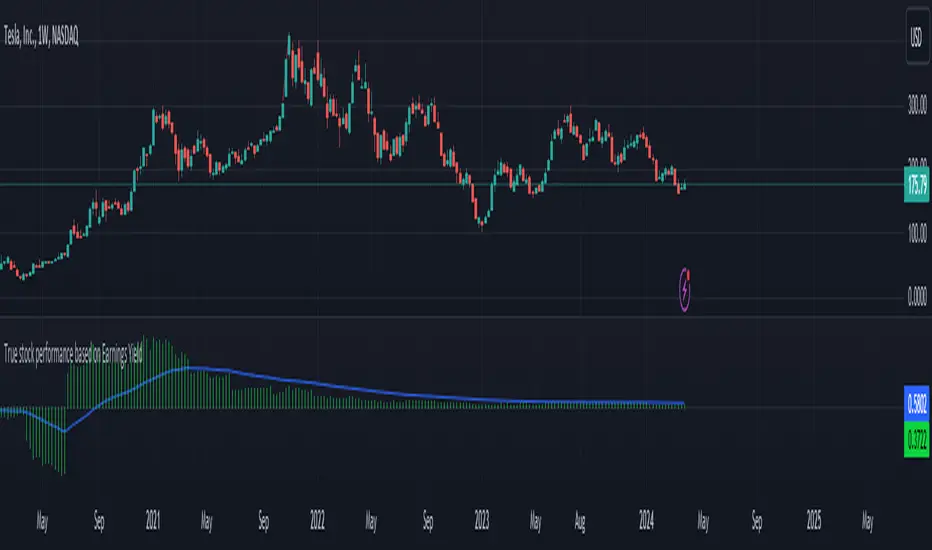
True stock performance based on Earnings YieldThe whole basis of the stock market is that you invest your money into a business that can use that money to increase it's earnings and pay you back for that investment with dividends and increased stock value. But because we are human the market often overbuy stocks that cant keep up their earnings with the current inflow of investments. We can also oversell a stock that is keeping up with earnings in regards to the stock price but we don't care because of the sentiment we have.
Earnings Yield is simply the percentage of Earnings Per Share in relation to the stock price. Alone, it's a great fundamental indicator to analyze a company. But I wanted to use it in another way and got tired of using the calculator all the time so that's why I made this indicator.
The goal is to see if the STOCK price is moving accordingly to the BUSINESS earnings. It works by calculating the difference of EY (TTM) previous close (1 bar) to the close thereafter. It then calculates the stock performance of the latest bar and divides that to get decimal form instead of percent. Then it divides the stock performance in decimal form with the difference of EY calculated before. The result shows how much the stock prices moves in relation to how much EY is moving. The theory is that if EY barely moves but the stock price moves heavily, you have a sentiment driven trend.
Example: Week 1 EY = 1.201. Week 2 EY = 1.105.
1.201 - 1.105 = 0.096
Week 2 performed a 11,2% increase in stock price. = 0.112 in decimal form.
0.112 / 0.096 = 1.67
1.67 is the multiple that plots this indicator.
Here is an good example of a stock that's currently in a highly sentiment driven trend, NVIDIA! (Posted 2024-03-30)
Here is an example of a Swedish stock that retail investors flocked to that have been blowned out completely.
When do I buy and sell?
This indicator is not meant to give exact entries or exits. The purpose is to scout the current and past sentiment, possible divergencies and see if a stock is over or under valued. I did add a 50 EMA to get some form of mean plotted. One could buy when true performance is low and sell when true performance drops below the 50 EMA. You could also just sell a part of your position and set a trailing exit with a ordinary 50 EMA or something like that. Often the sentiment will keep driving the price up. But if it last for 1 month or 1 year is impossible to tell.
Try it out and learn how it works and use it as you like. Cheers!
RSI Strategy with Manual TP and SL 19/03/2024This TradingView script implements a simple RSI (Relative Strength Index) strategy with manual take profit (TP) and stop-loss (SL) levels. Let's break down the script and analyze its components:
RSI Calculation: The script calculates the RSI using the specified length parameter. RSI is a momentum oscillator that measures the speed and change of price movements. It ranges from 0 to 100 and typically values above 70 indicate overbought conditions while values below 30 indicate oversold conditions.
Strategy Parameters:
length: Length of the RSI period.
overSold: Threshold for oversold condition.
overBought: Threshold for overbought condition.
trail_profit_pct: Percentage for trailing profit.
Entry Conditions:
For a long position: RSI crosses above 30 and the daily close is above 70% of the highest close in the last 50 bars.
For a short position: RSI crosses below 70 and the daily close is below 130% of the lowest close in the last 50 bars.
Entry Signals:
Long entry is signaled when both conditions for a long position are met.
Short entry is signaled when both conditions for a short position are met.
Manual TP and SL:
Take profit and stop-loss levels are calculated based on the entry price and the specified percentage.
For long positions, the take profit level is set above the entry price and the stop-loss level is set below the entry price.
For short positions, the take profit level is set below the entry price and the stop-loss level is set above the entry price.
Strategy Exits:
Exit conditions are defined for both long and short positions using the calculated take profit and stop-loss levels.
Chart Analysis:
This strategy aims to capitalize on short-term momentum shifts indicated by RSI crossings combined with daily price movements.
It utilizes manual TP and SL levels, providing traders with flexibility in managing their positions.
The strategy may perform well in ranging or oscillating markets where RSI signals are more reliable.
However, it may encounter challenges in trending markets where RSI can remain overbought or oversold for extended periods.
Traders should backtest this strategy thoroughly on historical data and consider optimizing parameters to suit different market conditions.
Risk management is crucial, so traders should carefully adjust TP and SL percentages based on their risk tolerance and market volatility.
Overall, this strategy provides a structured approach to trading based on RSI signals while allowing traders to customize their risk management. However, like any trading strategy, it should be used judiciously and in conjunction with other forms of analysis and risk management techniques.

Ichimoku OscillatorHello All,
This is Ichimoku Oscillator that creates different oscillator layers, calculates the trend and possible entry/exit levels by using Ichimoku Cloud features.
There are four layer:
First layer is the distance between closing price and cloud (min or max, depending on the main trend)
Second layer is the distance between Lagging and Cloud X bars ago (X: the displacement)
Third layer is the distance between Conversion and Base lines
Fourth layer is the distance between both Leadlines
If all layers are visible maning that positive according to the main trend, you can take long/short position and when main trend changed then you should close the position. so it doesn't mean you can take position when main trend changed, you need to wait for all other conditions met (all layers(
there is take profit partially option. if Conversion and base lines cross then you can take profit partially. Optionally you can take profit partially when EMA line crosses Fourth layer.
Optionally ATR (average true range) is used for Conversion and baseline for protection from whipsaws. you can use it to stay on the trend longer time.
I added options to enable/disable the alert and customize alert messages. You can change alert messages as you wish. if you use ' close ' in the alert message then you can get closing price in the alert message when the alert was triggered.
There is an option Bounce Off Support/Resistance , if there is trend and if the price bounce off Support/Resistance zone then a tiny triangle is shown.
There are many other options for coloring, alerts etc.
Some screenshots:
Main trend:
Taking/closing positions:
Example alert messages:
Bounce off:
Colors:
Colors:
Colors:
Non-colored background:
P.S. For a few months I haven't published any new script because of some health issues. hope to be healthy and create new scripts in 2024 :)
Enjoy!

Volume Heatmap 2024 | NXT2017 Christmas EditionHi big players around the world,
I wish you a merry christmas time.
Today I have a nice present for you: a new volume heatmap indicator for free using!
HISTORY
My first volume heatmap project got a lot of feedback and a big demand. You can find it here:
In this time pinescript version 4 was the newest one and I worked the first time with arrays.
Today we have pinescript version 5 and some new features. This is why I tried again with matrix function and the results are better than I expected.
HOW IT WORKS
The indicator calculates similar like the volume profile. It looks back and every volume where the close price is on the same row area, the volume will cumulated. How much rows the new chart view is showing, you can choose manually.
The mind behind this is to find high volume levels, where high volume catch the price in a range or get function as support/resistance line.
PICTURES
I hope it helps for your trading. You are welcome to give some comments.
Merry christmas and best regards
NXT2017

chrono_utilsLibrary "chrono_utils"
📝 Description
Collection of objects and common functions that are related to datetime windows session days and time ranges. The main purpose of this library is to handle time-related functionality and make it easy to reason about a future bar checking if it will be part of a predefined session and/or inside a datetime window. All existing session functionality I found in the documentation e.g. "not na(time(timeframe, session, timezone))" are not suitable for strategy scripts, since the execution of the orders is delayed by one bar, due to the script execution happening at the bar close. Moreover, a history operator with a negative value that looks forward is not allowed in any pinescript expression. So, a prediction for the next bar using the bars_back argument of "time()"" and "time_close()" was necessary. Thus, I created this library to overcome this small but very important limitation. In the meantime, I added useful functionality to handle session-based behavior. An interesting utility that emerged from this development is data anomaly detection where a comparison between the prediction and the actual value is happening. If those two values are different then a data inconsistency happens between the prediction bar and the actual bar (probably due to a holiday, half session day, a timezone change etc..)
🤔 How to Guide
To use the functionality this library provides in your script you have to import it first!
Copy the import statement of the latest release by pressing the copy button below and then paste it into your script. Give a short name to this library so you can refer to it later on. The import statement should look like this:
import jason5480/chrono_utils/2 as chr
To check if a future bar will be inside a window first of all you have to initialize a DateTimeWindow object.
A code example is the following:
var dateTimeWindow = chr.DateTimeWindow.new().init(fromDateTime = timestamp('01 Jan 2023 00:00'), toDateTime = timestamp('01 Jan 2024 00:00'))
Then you have to "ask" the dateTimeWindow if the future bar defined by an offset (default is 1 that corresponds th the next bar), will be inside that window:
// Filter bars outside of the datetime window
bool dateFilterApproval = dateTimeWindow.is_bar_included()
You can visualize the result by drawing the background of the bars that are outside the given window:
bgcolor(color = dateFilterApproval ? na : color.new(color.fuchsia, 90), offset = 1, title = 'Datetime Window Filter')
In the same way, you can "ask" the Session if the future bar defined by an offset it will be inside that session.
First of all, you should initialize a Session object.
A code example is the following:
var sess = chr.Session.new().from_sess_string(sess = '0800-1700:23456', refTimezone = 'UTC')
Then check if the given bar defined by the offset (default is 1 that corresponds th the next bar), will be inside the session like that:
// Filter bars outside the sessions
bool sessionFilterApproval = view.sess.is_bar_included()
You can visualize the result by drawing the background of the bars that are outside the given session:
bgcolor(color = sessionFilterApproval ? na : color.new(color.red, 90), offset = 1, title = 'Session Filter')
In case you want to visualize multiple session ranges you can create a SessionView object like that:
var view = SessionView.new().init(SessionDays.new().from_sess_string('2345'), array.from(SessionTimeRange.new().from_sess_string('0800-1600'), SessionTimeRange.new().from_sess_string('1300-2200')), array.from('London', 'New York'), array.from(color.blue, color.orange))
and then call the draw method of the SessionView object like that:
view.draw()
🏋️♂️ Please refer to the "EXAMPLE DATETIME WINDOW FILTER" and "EXAMPLE SESSION FILTER" regions of the script for more advanced code examples of how to utilize the full potential of this library, including user input settings and advanced visualization!
⚠️ Caveats
As I mentioned in the description there are some cases that the prediction of the next bar is not accurate. A wrong prediction will affect the outcome of the filtering. The main reasons this could happen are the following:
Public holidays when the market is closed
Half trading days usually before public holidays
Change in the daylight saving time (DST)
A data anomaly of the chart, where there are missing and/or inconsistent data.
A bug in this library (Please report by PM sending the symbol, timeframe, and settings)
Special thanks to @robbatt and @skinra for the constructive feedback 🏆. Without them, the exposed API of this library would be very lengthy and complicated to use. Thanks to them, now the user of this library will be able to get the most, with only a few lines of code!

Bitcoin Stock to FlowModeling Bitcoin's Value With Scarcity
The Stock to Flow model for Bitcoin suggests that Bitcoin price is driven by scarcity over time.
Bitcoin is the first scarce digital object the world has ever seen. It is scarce like silver & gold, and can be sent over the internet, radio, satellite etc. Bitcoin includes a mathematical mechanism to restrict its supply over time making it more rare as time goes on. Digital Scarcity.
In 2017 BTC exceeded the market capitalization of Silver. After the next halving in 2024, Bitcoin will become the hardest asset the world has ever seen, rarer than Gold.
There is only enough Bitcoin in the world for each person to own .0023 BTC. Because of this, Bitcoin's value should continue to rise over time.