whookLibrary "whook"
This library provides functions for generating trading alerts for `whook`
check this -> github.com
Currently supported exchanges:
Kucoin futures
Bitget futures
Coinex futures
Bingx
OKX futures ( also its demo mode )
Bybit futures ( also Bybit testnet )
Binance futures ( also Binance futures testnet )
Phemex futures ( also Phemex testnet )
Kraken futures ( also Kraken futures testnet )
# --- Test Cases ---
Note: These test cases are for demonstration purposes only and may not cover all scenarios.
// buy(string account, float amount, string unit = "units", float leverage = 1)
buy("MyAccount", 100, "units", 1)
buy("MyAccount", 1000, "USDT", 5)
buy("MyAccount", 50, "percent", 2)
// sell(string account, float amount, string unit = "units", float leverage = 1)
sell("MyAccount", 50, "units", 1)
sell("MyAccount", 500, "USDT", 3)
sell("MyAccount", 25, "percent", 2)
// set_position(string account, float amount, string unit = "units", float leverage = 1)
set_position("MyAccount", 100, "units", 1)
set_position("MyAccount", 1000, "USDT", 5)
set_position("MyAccount", 50, "percent", 2)
// limit_buy(string account, float amount, float price, string unit = "units", float leverage = 1, string id = "")
limit_buy("MyAccount", 100, 10000, "units", 1, "MyBuyOrder")
limit_buy("MyAccount", 1000, 10500, "USDT", 5)
limit_buy("MyAccount", 50, 11000, "percent", 2)
// limit_sell(string account, float amount, float price, string unit = "units", float leverage = 1, string id = "")
limit_sell("MyAccount", 50, 10000, "units", 1, "MySellOrder")
limit_sell("MyAccount", 500, 9500, "USDT", 3)
limit_sell("MyAccount", 25, 9000, "percent", 2)
// close_percent(string account, float pct = 100)
close_percent("MyAccount", 100)
close_percent("MyAccount", 50)
buy(account, amount, unit, leverage)
Sends a trading alert to execute a market buy order.
Parameters:
account (string) : The account ID.
amount (float) : The amount to buy (can be in USD, units, or percentage).
unit (string) : The unit of the amount (optional, defaults to "units").
leverage (float) : The leverage to use (optional, defaults to 1x).
sell(account, amount, unit, leverage)
Sends a trading alert to execute a market sell order.
Parameters:
account (string) : The account ID.
amount (float) : The amount to sell (can be in USD, units, or percentage).
unit (string) : The unit of the amount (optional, defaults to "units").
leverage (float) : The leverage to use (optional, defaults to 1x).
set_position(account, amount, unit, leverage)
Sends a trading alert to set a position.
Parameters:
account (string) : The account ID.
amount (float) : The amount to set the position to (can be in USD, units, or percentage).
unit (string) : The unit of the amount (optional, defaults to "units").
leverage (float) : The leverage to use (optional, defaults to 1x).
limit_buy(account, amount, price, unit, leverage, id)
Sends a trading alert to place a limit buy order.
Parameters:
account (string) : The account ID.
amount (float) : The amount to buy (can be in USD, units, or percentage).
price (float) : The limit price.
unit (string) : The unit of the amount (optional, defaults to "units").
leverage (float) : The leverage to use (optional, defaults to 1x).
id (string) : An optional custom ID for the limit order.
limit_sell(account, amount, price, unit, leverage, id)
Sends a trading alert to place a limit sell order.
Parameters:
account (string) : The account ID.
amount (float) : The amount to sell (can be in USD, units, or percentage).
price (float) : The limit price.
unit (string) : The unit of the amount (optional, defaults to "units").
leverage (float) : The leverage to use (optional, defaults to 1x).
id (string) : An optional custom ID for the limit order.
close_percent(account, pct)
Sends an alert to close a position on Phemex.
Parameters:
account (string) : The account ID.
pct (float) : The percentage of the position to close (optional, defaults to 100%).
Cerca negli script per "100年黄金价格走势"

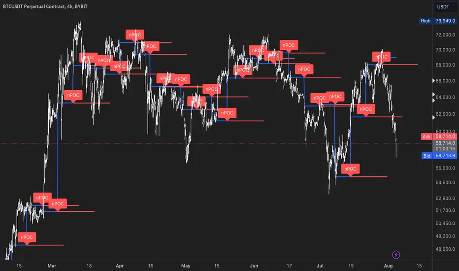
nPOC Levels by Tyler### Explanation of the Pine Script
This Pine Script identifies and displays weekly naked Points of Control (nPOCs) on a TradingView chart. An nPOC represents a Point of Control (POC) from a previous week that has not been revisited by price action in subsequent weeks. These nPOCs are extended to the right as horizontal lines, indicating potential support or resistance levels.
#### Script Overview
1. **Indicator Declaration:**
```pinescript
//@version=5
indicator("Weekly nPOCs", overlay=true)
```
- The script is defined as a version 5 Pine Script.
- The `indicator` function sets the script's name ("Weekly nPOCs") and specifies that the indicator should be overlaid on the price chart (`overlay=true`).
2. **Function to Calculate POC:**
```pinescript
f_poc(_hl2, _vol) =>
var float vol_profile = na
if (na(vol_profile))
vol_profile := array.new_float(100, 0.0)
_bin_size = (high - low) / 100
for i = 0 to 99
if _hl2 >= low + i * _bin_size and _hl2 < low + (i + 1) * _bin_size
array.set(vol_profile, i, array.get(vol_profile, i) + _vol)
max_volume = array.max(vol_profile)
poc_index = array.indexof(vol_profile, max_volume)
poc_price = low + poc_index * _bin_size + _bin_size / 2
poc_price
```
- The function `f_poc` calculates the Point of Control (POC) for a given period.
- It takes two parameters: `_hl2` (the average of the high and low prices) and `_vol` (volume).
- A volume profile array (`vol_profile`) is initialized to store volume data across different price bins.
- The price range between the high and low is divided into 100 bins (`_bin_size`).
- The function iterates over each bin, accumulating the volumes for prices within each bin.
- The bin with the maximum volume is identified as the POC (`poc_price`).
3. **Variables to Store Weekly Data:**
```pinescript
var float poc = na
var float prev_poc = na
var line poc_lines = na
if na(poc_lines)
poc_lines := array.new_line(0)
```
- `poc` stores the current week's POC.
- `prev_poc` stores the previous week's POC.
- `poc_lines` is an array to store lines representing nPOCs. The array is initialized if it is `na` (not initialized).
4. **Calculate Weekly POC:**
```pinescript
is_new_week = ta.change(time('W')) != 0
if (is_new_week)
prev_poc := poc
poc := f_poc(hl2, volume)
if not na(prev_poc)
line new_poc_line = line.new(x1=bar_index, y1=prev_poc, x2=bar_index + 100, y2=prev_poc, color=color.red, width=2)
label.new(x=bar_index, y=prev_poc, text="nPOC", style=label.style_label_down, color=color.red, textcolor=color.white)
array.push(poc_lines, new_poc_line)
```
- `is_new_week` checks if the current bar is the start of a new week using the `ta.change(time('W'))` function.
- If it's a new week, the previous week's POC is stored in `prev_poc`, and the current week's POC is calculated using `f_poc`.
- If `prev_poc` is not `na`, a new line (`new_poc_line`) representing the nPOC is created, extending it to the right (for 100 bars).
- A label is created at the `prev_poc` level, marking it as "nPOC".
- The new line is added to the `poc_lines` array.
5. **Remove Old Lines:**
```pinescript
if array.size(poc_lines) > 52
line.delete(array.shift(poc_lines))
```
- This section ensures that only the last 52 weeks of nPOCs are kept to avoid cluttering the chart.
- If the `poc_lines` array contains more than 52 lines, the oldest line is deleted using `array.shift`.
6. **Plot the Current Week's POC as a Reference:**
```pinescript
plot(poc, title="Current Weekly POC", color=color.blue, linewidth=2, style=plot.style_line)
```
- The current week's POC is plotted as a blue line on the chart for reference.
#### Summary
This script calculates and identifies weekly Points of Control (POCs) and marks them as nPOCs if they remain untouched by subsequent price action. These nPOCs are displayed as horizontal lines extending to the right, providing traders with potential support or resistance levels. The script also manages the number of lines plotted to maintain a clear and uncluttered chart.
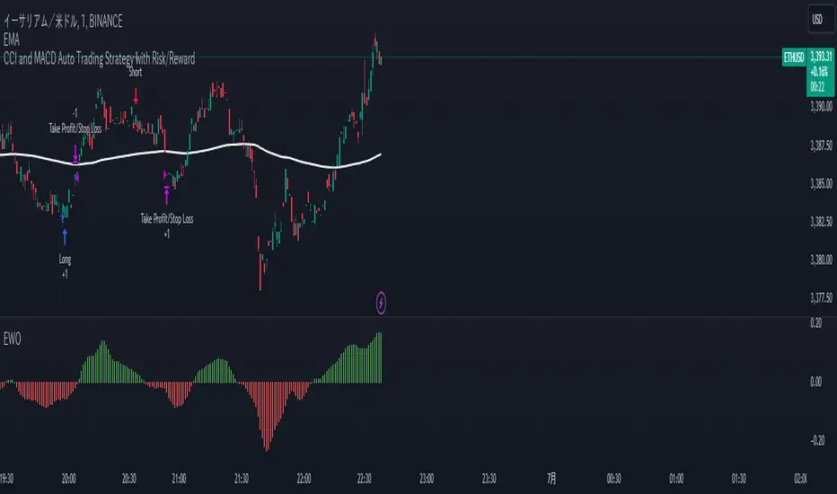
CCI and MACD Auto Trading Strategy with Risk/RewardOverview:
This strategy combines the Commodity Channel Index (CCI) and the Moving Average Convergence Divergence (MACD) indicators to automate trading decisions. It dynamically sets stop-loss and take-profit levels based on recent lows and highs, ensuring a risk/reward ratio of 1:1.5. This script aims to leverage trend and momentum signals while maintaining effective risk management.
Originality and Usefulness:
This script is not just a simple mashup of CCI and MACD indicators; it incorporates dynamic risk management by setting stop-loss and take-profit levels based on recent price action. This approach helps traders to:
・Identify potential trend reversals using the combination of CCI and MACD signals.
・Manage trades effectively by setting realistic stop-loss and take-profit levels based on recent market data.
・Maintain a balanced risk/reward ratio, which is essential for sustainable trading.
Indicators Used:
・CCI (Commodity Channel Index):
・Measures the deviation of the price from its average over a specified period, typically ranging from -100 to +100.
・Helps identify overbought and oversold conditions.
・MACD (Moving Average Convergence Divergence):
・Utilizes the difference between short-term and long-term moving averages to indicate trend strength and direction.
・Provides momentum signals that can be used for timing entries and exits.
How It Works:
Entry Conditions:
Long Entry:
・The MACD histogram is above zero.
・The CCI crosses above the -100 line.
Short Entry:
・The MACD histogram is below zero.
・The CCI crosses below the +100 line.
Exit Conditions:
Long Positions:
・The stop-loss is set at the recent low.
・The take-profit is set at 1.5 times the distance between the entry price and the stop-loss.
Short Positions:
・The stop-loss is set at the recent high.
・The take-profit is set at 1.5 times the distance between the entry price and the stop-loss.
Risk Management:
・The script dynamically adjusts stop-loss and take-profit levels based on recent market data, ensuring that the risk/reward ratio is maintained at 1:1.5.
・This approach helps in managing the risk effectively while aiming for consistent profits.
Strategy Properties:
・Account Size: Configured for a realistic account size suitable for the average trader.
・Commission and Slippage: Includes settings for realistic commission and slippage to reflect real market conditions.
・Risk per Trade: Designed to risk no more than 5-10% of equity per trade, aligning with sustainable trading practices.
・Backtesting Results: Configured to generate a sufficient sample size (ideally more than 100 trades) for reliable backtesting results.
Revised Backtesting Settings
Ensure that your backtesting settings are realistic:
・Account Size: Set a realistic initial capital suitable for the average trader.
・Commission and Slippage: Include realistic commission fees and slippage.
・Risk Management: Ensure that each trade risks no more than 5-10% of the account equity.
・Sufficient Sample Size: Choose a dataset that will generate more than 100 trades to provide a robust sample size.
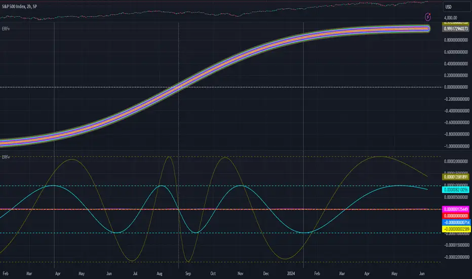
[Pandora] Error Function Treasure Trove - ERF/ERFI/Sigmoids+PRAISE:
At this time, I have to graciously thank the wonderful minds behind the new "Pine Profiler Mode" (PPM). Directly prior to this release, it allowed me to ascertain script performance even more. While I usually write mostly in highly optimized Pine code, PPM visually identified a few bottlenecks that would otherwise be hard to identify. Anyone who contributed to PPMs creation and testing before release... BRAVO!!! I commend all of those who assisted in it's state-of-the-art engineering and inception, well done!
BACKSTORY:
This script is specifically being released in defense of another member, an exceptionally unique PhD. It was brought to my attention that a script-mod-event occurred, regarding the publishing of a measly antiquated error function (ERF) calculation within his script. This sadly resulted in the now former member jumping ship after receiving unmannerly responses amidst his curious inquiries as to why his erf() was modded. To forbid rusty and rudimentary formulations because a mod-on-duty is temporally offended by a non-nefarious release of code, is in MY opinion an injustice to principles of perpetuating open-source code intended to benefit thousands to millions of community members. While Pine is the heart and soul of TV, the mathematical concepts contributed from the minds of members is the inspirational fuel of curiosity that powers it's pertinent reason to exist and evolve.
It is an indisputable fact that most members are not greatly skilled Pine Poets. Many members may be incapable of innovating robust function code in Pine, even if they have one or more PhDs. We ALL come from various disciplines of mathematical comprehension and education. Some mathematicians are not greatly skilled at coding, while some coders are not exceptional at math. So... what am I to do to attempt to resolve this circumstantial challenge??? Those who know me best are aware that I will always side with "the right side of history" in order to accomplish my primary self-defined missions I choose to accept. Serving as an algorithmic advocate, I felt compelled to intercede by compiling numerous error functions into elegant code of very high caliber that any and every TV member may choose to employ, so this ERROR never happens again.
After weeks of contemplation into algorithms I knew little about, I prioritized myself to resolve an unanticipated matter by creating advanced formulas of exquisitely crafted error functions refined to the best of my current abilities. My aversion for unresolved problems motivated me to eviscerate error function insufficiencies with many more rigid formulations beyond what is thought to exist. ERF needed a proper algorithmic exorcism anyways. In my furiosity, I contemplated an array of madMAXimum diplomatic demolition methods, choosing the chain saw massacre technique to slaughter dysfunctionalities I encountered on a battered ERF roadway. This resulted in prolific solutions that should assuredly endure the test of time. Poetically, as you will come to see, I am ripping the lid off of Pandora's box of error functions in this case to correct wrongs into a splendid bundle of rights for members.
INTENTION:
Error function (ERF) enthusiasts... PREPARE FOR GLORY!! The specific purpose of this script is to deprecate classic error functions with the creation of a fierce and formidable army of superior formulations, each having varying attributes of computational complexity with differing absolute error ranges in their results for multiple compute scenarios. This is NOT an indicator... It is intended to allow members to embark on endeavors to advance the profound knowledge base of this growing worldwide community of 60+ million inquisitive minds. For those of you who believe computational mathematics and statistics is near completion at its finest; I am here to inform you, this is ridiculous to ponder. We are no where near statistical excellence that can and will exist eventually. At this time, metaphorically speaking, we are merely scratching microns off of the surface of the skin of a statistical apple Isaac Newton once pondered.
THIS RELEASE:
Following weeks of pondering methodical experiments beyond the ordinary, I am liberating these wild notions of my error function explorations to the entire globe as copyleft code, not just Pine. This Pandora's basket of ERFs is being openly disclosed for the sake of the sanctity of mathematics, empirical science (not the garbage we are told by CONTROLocrats to blindly trust), revolutionary cutting edge engineering, cosmology, physics, information technology, artificial intelligence, and EVERY other mathematical branch of human knowledge being discovered over centuries. I do believe James Glaisher would favor my aims concerning ERF aspirations embracing the "Power of Pine".
The included functions are intended for TV members to use in any way they see fit. This is a gift to ALL members to foster future innovative excellence on this platform. Any attempt to moderate this code without notification of "self-evident clear and just cause" will be considered an irrevocable egregious action. The original foundational PURPOSE of establishing script moderation (I clearly remember) was primarily to maintain active vigilance over a growing community against intentional nefarious actions and/or behaviors in blatant disrespect to other author's works AND also thwart rampant copypasting bandit operations, all while accommodating balanced principles of fairness for an educational community cause via open source publishing that should support future algorithmic inventions well beyond my lifespan.
APPLICATIONS:
The related error functions are used in probability theory, statistics, and numerous and engineering scientific disciplines. Its key characteristics and applications are innumerable in computational realms. Its versatility and significance make it a fundamental tool in arenas of quantitative analysis and scientific research...
Probability Theory - Is widely used in probability theory to calculate probabilities and quantiles of the normal distribution.
Statistics - It's related to the Gaussian integral and plays a crucial role in statistics, especially in hypothesis testing and confidence interval calculations.
Physics - In physics, it arises in the study of diffusion equations, quantum mechanics, and heat conduction problems.
Engineering - Applications exist in engineering disciplines such as signal processing, control theory, and telecommunications.
Error Analysis - It's employed in error analysis and uncertainty quantification.
Numeric Approximations - Due to its lack of a closed-form expression, numerical methods are often employed to approximate erf/erfi().
AI, LLMs, & MACHINE LEARNING:
The error function (ERF) is indispensable to various AI applications, particularly due to its relation to Gaussian distributions and error analysis. It is used in Gaussian processes for regression and classification, probabilistic inference for Bayesian networks, soft margin computation in SVMs, neural networks involving Gaussian activation functions or noise, and clustering algorithms like Gaussian Mixture Models. Improved ERF approximations can enhance precision in these applications, reduce computational complexity, handle outliers and noise better, and improve optimization and convergence, possibly leading to more accurate, efficient, and robust AI systems.
BONUS ALGORITHMS:
While ERFs are versatile, its opposite also exists in the form of inverse error functions (ERFIs). I have also included a modified form of the inverse fisher transform along side MY sigmoid (sigmyod). I am uncertain what sigmyod() may be used for, but it's a culmination of my examinations deep into "sigmoid domains", something I am fascinated by. Whatever implications it may possess, I am unveiling it along with it's cousin functions. For curious minds, this quality of composition seen here is ideally what underlies what I would term "Pandora functionality" that empowers my Pandora indication. I go through hordes of formulations, testing, and inspection to find what appears to be the most beneficial logical/mathematical equation to apply...
SCRIPT OPERATION:
To showcase the characteristics and performance of my ERF/ERFI formulations, I devised a multi-modal script. By using bar_index , I generated a broad sequence of numeric values to input into the first ERF/ERFI parameter. These sequences allow you to inspect the contours of the error function's outputs for both ERF and ERFI. When combined with compute-intensive precision functions (CIPFs), the polynomial function output values can be subtracted from my CIPFs to obtain results of absolute error, displaying the accuracy of the many polynomial estimation functions I tuned in testing for Pine's float environment.
A host of numeric input settings are wildly adjustable to inspect values/curvatures across the range of numeric input sequences. Very large numbers, such as Divisor:100,000,100/Offset:200,000,000 for ERF modes or... Divisor:100,000,100/Offset:100,000,000 for ERFI modes, will display miniscule output values calculated from input values in close proximity to 0.0 for the various estimates, similar to a microscope. ERFI approximations very near in proximity to +/-1.0 will always yield large deviations of absolute error. Dragging/zooming your chart or using the Offset input will aid with visually clipping off those ERFI extremes where float precision functions cannot suffice.
NOTICE:
perf() and perfi() are intended for precision computation (as good as it basically gets) in a float environment. However, they are CPU intensive (especially perfi). I wouldn't recommend these being used in ANY Pine script unless it's an "absolute necessity" to do so to accomplish your goal. I only built them to obtain "absolute error curvatures" of the error functions for the polynomial approximations. These are visible in the accuracy modes in the indicator Settings.
ATE_Common_Functions_LibraryLibrary "ATE_Common_Functions_Library"
- ATE_Common_Functions_Library was created to assist in constructing CCOMET Scanners
RCI(_rciLength, _source, _interval)
You will see me using this a lot. DEFINITELY my favorite oscillator to utilize for SO many different things from
timing entries/exits to determining trends.Calculation of this indicator based on Spearmans Correlation.
Parameters:
_rciLength (int) : (int)
Amount of bars back to use in RCI calculations.
_source (float) : (float)
Source to use in RCI calculations (can use ANY source series. Ie, open,close,high,low,etc).
_interval (int) : (int)
Optional (if parameter not included, it defaults to 3). RCI calculation groups bars by this amount and then will.
rank these groups of bars.
Returns: (float)
Returns a single RCI value that will oscillates between -100 and +100.
RCIAVG(_rciSMAlen, _source, _interval, firstLength, lastLength)
20 RCI's are averaged together to get this RCI Avg (Rank Correlation Index Average). Each RCI (of the 20 total RCI)
has a progressively LARGER Lookback Length. Rather than having ALL of the RCI Lengths be individually adjustable (because of too many inputs),
I have made the FIRST Length used (smallest Length value in the set) and the LAST Length used (largest length value in the set) be adjustable
and all other 18 Lengths are equally spread out between the 'firstLength' and the 'lastLength'.
Parameters:
_rciSMAlen (int) : (int)
Unlike the Single RCI Function, this function smooths out the end result using an SMA with a length value that is this parameter.
_source (float) : (float)
Source to use in RCI calculations (can use ANY source series. Ie, open,close,high,low,etc).
_interval (int) : (int)
Optional (if parameter not included, it defaults to 3). Within the RCI calculation, bars next to each other are grouped together
and then these groups are Ranked against each other. This parameter is the number of adjacent bars that are grouped together.
firstLength (int) : (int)
Optional (if parameter is not included when the function is called on in the script, then it defaults to 200).
This parameter is the Lookback Length for the 1st RCI used (so the SMALLEST Length used) in the RCI Avg.
lastLength (int) : (int)
Optional (if parameter is not included when the function is called on in the script, then it defaults to 2500).
This parameter is the Lookback Length for the 20th(the LAST) RCI used (so the LARGEST Length used) in the RCI Avg.
***** BEWARE ***** The 'lastLength' must be less than (or possibly equal to) 5000 because Tradingview has capped it at 5000, causing an error.
***** BEWARE ***** If the script gives a compiler "time out" error then the 'lastLength' must be lowered until it no longer times out when compiling.
Returns: (float)
Returns a single RCI value that is the Avg of many RCI values that will oscillate between -100 and +100.
PercentChange(_startingValue, _endingValue)
This is a quick function to calculate how much % change has occurred between the '_startingValue' and the '_endingValue'
that you input into the function.
Parameters:
_startingValue (float) : (float)
The source value to START the % change calculation from.
_endingValue (float) : (float)
The source value to END the % change caluclation from.
Returns: Returns a single output being the % value between 0-100 (with trailing numbers behind a decimal). If you want only
a certain amount of numbers behind the decimal, this function needs to be put within a formatting function to do so.
Rescale(_source, _oldMin, _oldMax, _newMin, _newMax)
Rescales series with a known '_oldMin' & '_oldMax'. Use this when the scale of the '_source' to
rescale is known (bounded).
Parameters:
_source (float) : (float)
Source to be normalized.
_oldMin (int) : (float)
The known minimum of the '_source'.
_oldMax (int) : (float)
The known maximum of the '_source'.
_newMin (int) : (float)
What you want the NEW minimum of the '_source' to be.
_newMax (int) : (float)
What you want the NEW maximum of the '_source' to be.
Returns: Outputs your previously bounded '_source', but now the value will only move between the '_newMin' and '_newMax'
values you set in the variables.
Normalize_Historical(_source, _minimumLvl, _maximumLvl)
Normalizes '_source' that has a previously unknown min/max(unbounded) determining the max & min of the '_source'
FROM THE ENTIRE CHARTS HISTORY. ]
Parameters:
_source (float) : (float)
Source to be normalized.
_minimumLvl (int) : (float)
The Lower Boundary Level.
_maximumLvl (int) : (float)
The Upper Boundary Level.
Returns: Returns your same '_source', but now the value will MOSTLY stay between the minimum and maximum values you set in the
'_minimumLvl' and '_maximumLvl' variables (ie. if the source you input is an RSI...the output is the same RSI value but
instead of moving between 0-100 it will move between the maxand min you set).
Normailize_Local(_source, _length, _minimumLvl, _maximumLvl)
Normalizes series with previously unknown min/max(unbounded). Much like the Normalize_Historical function above this one,
but rather than using the Highest/Lowest Values within the ENTIRE charts history, this on looks for the Highest/Lowest
values of '_source' within the last ___ bars (set by user as/in the '_length' parameter. ]
Parameters:
_source (float) : (float)
Source to be normalized.
_length (int) : (float)
The amount of bars to look back to determine the highest/lowest '_source' value.
_minimumLvl (int) : (float)
The Lower Boundary Level.
_maximumLvl (int) : (float)
The Upper Boundary Level.
Returns: Returns a single output variable being the previously unbounded '_source' that is now normalized and bound between
the values used for '_minimumLvl'/'_maximumLvl' of the '_source' within the user defined lookback period.
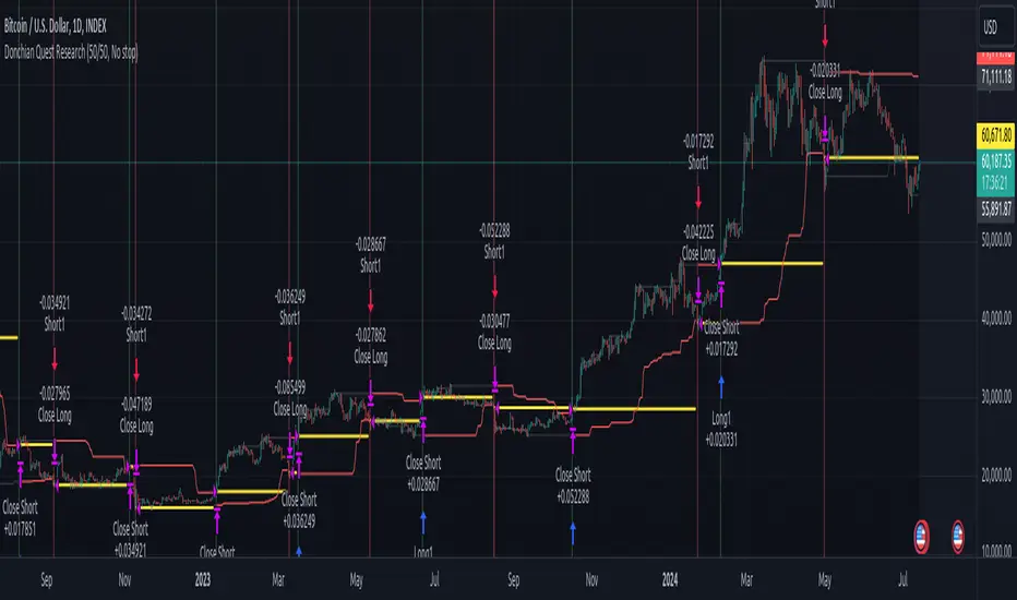
Donchian Quest Research// =================================
Trend following strategy.
// =================================
Strategy uses two channels. One channel - for opening trades. Second channel - for closing.
Channel is similar to Donchian channel, but uses Close prices (not High/Low). That helps don't react to wicks of volatile candles (“stop hunting”). In most cases openings occur earlier than in Donchian channel. Closings occur only for real breakout.
// =================================
Strategy waits for beginning of trend - when price breakout of channel. Default length of both channels = 50 candles.
Conditions of trading:
- Open Long: If last Close = max Close for 50 closes.
- Close Long: If last Close = min Close for 50 closes.
- Open Short: If last Close = min Close for 50 closes.
- Close Short: If last Close = max Close for 50 closes.
// =================================
Color of lines:
- black - channel for opening trade.
- red - channel for closing trade.
- yellow - entry price.
- fuchsia - stoploss and breakeven.
- vertical green - go Long.
- vertical red - go Short.
- vertical gray - close in end, don't trade anymore.
// =================================
Order size calculated with ATR and volatility.
You can't trade 1 contract in BTC and 1 contract in XRP - for example. They have different price and volatility, so 1 contract BTC not equal 1 contract XRP.
Script uses universal calculation for every market. It is based on:
- Risk - USD sum you ready to loss in one trade. It calculated as percent of Equity.
- ATR indicator - measurement of volatility.
With default setting your stoploss = 0.5 percent of equity:
- If initial capital is 1000 USD and used parameter "Permit stop" - loss will be 5 USD (0.5 % of equity).
- If your Equity rises to 2000 USD and used parameter "Permit stop"- loss will be 10 USD (0.5 % of Equity).
// =================================
This Risk works only if you enable “Permit stop” parameter in Settings.
If this parameter disabled - strategy works as reversal strategy:
⁃ If close Long - channel border works as stoploss and momentarily go Short.
⁃ If close Short - channel border works as stoploss and momentarily go Long.
Channel borders changed dynamically. So sometime your loss will be greater than ‘Risk %’. Sometime - less than ‘Risk %’.
If this parameter enabled - maximum loss always equal to 'Risk %'. This parameter also include breakeven: if profit % = Risk %, then move stoploss to entry price.
// =================================
Like all trend following strategies - it works only in trend conditions. If no trend - slowly bleeding. There is no special additional indicator to filter trend/notrend. You need to trade every signal of strategy.
Strategy gives many losses:
⁃ 30 % of trades will close with profit.
⁃ 70 % of trades will close with loss.
⁃ But profit from 30% will be much greater than loss from 70 %.
Your task - patiently wait for it and don't use risky setting for position sizing.
// =================================
Recommended timeframe - Daily.
// =================================
Trend can vary in lengths. Selecting length of channels determine which trend you will be hunting:
⁃ 20/10 - from several days to several weeks.
⁃ 20/20 or 50/20 - from several weeks to several months.
⁃ 50/50 or 100/50 or 100/100 - from several months to several years.
// =================================
Inputs (Settings):
- Length: length of channel for trade opening/closing. You can choose 20/10, 20/20, 50/20, 50/50, 100/50, 100/100. Default value: 50/50.
- Permit Long / Permit short: Longs are most profitable for this strategy. You can disable Shorts and enable Longs only. Default value: permit all directions.
- Risk % of Equity: for position sizing used Equity percent. Don't use values greater than 5 % - it's risky. Default value: 0.5%.
⁃ ATR multiplier: this multiplier moves stoploss up or down. Big multiplier = small size of order, small profit, stoploss far from entry, low chance of stoploss. Small multiplier = big size of order, big profit, stop near entry, high chance of stoploss. Default value: 2.
- ATR length: number of candles to calculate ATR indicator. It used for order size and stoploss. Default value: 20.
- Close in end - to close active trade in the end (and don't trade anymore) or leave it open. You can see difference in Strategy Tester. Default value: don’t close.
- Permit stop: use stop or go reversal. Default value: without stop, reversal strategy.
// =================================
Properties (Settings):
- Initial capital - 1000 USD.
- Script don't uses 'Order size' - you need to change 'Risk %' in Inputs instead.
- Script don't uses 'Pyramiding'.
- 'Commission' 0.055 % and 'Slippage' 0 - this parameters are for crypto exchanges with perpetual contracts (for example Bybit). If use on other markets - set it accordingly to your exchange parameters.
// =================================
Big dataset used for chart - 'BITCOIN ALL TIME HISTORY INDEX'. It gives enough trades to understand logic of script. It have several good trends.
// =================================
A_Traders_Edge__LibraryLibrary "A_Traders_Edge__Library"
- A Trader's Edge (ATE)_Library was created to assist in constructing Market Overview Scanners (MOS)
LabelLocation(_firstLocation)
This function is used when there's a desire to print an assets ALERT LABELS at a set location on the scale that will
NOT change throughout the progression of the script. This is created so that if a lot of alerts are triggered, they
will stay relatively visible and not overlap each other. Ex. If you set your '_firstLocation' parameter as 1, since
there are a max of 40 assets that can be scanned, the 1st asset's location is assigned the value in the '_firstLocation' parameter,
the 2nd asset's location is the (1st asset's location+1)...and so on. If your first location is set to 81 then
the 1st asset is 81 and 2nd is 82 and so on until the 40th location = 120(in this particular example).
Parameters:
_firstLocation (simple int) : (simple int)
Optional(starts at 1 if no parameter added).
Location that you want the first asset to print its label if is triggered to do so.
ie. loc2=loc1+1, loc3=loc2+1, etc.
Returns: Returns 40 output variables each being a different location to print the labels so that an asset is asssigned to
a particular location on the scale. Regardless of if you have the maximum amount of assets being screened (40 max), this
function will output 40 locations… So there needs to be 40 variables assigned in the tuple in this function. What I
mean by that is you need to have 40 output location variables within your tuple (ie. between the ' ') regarless of
if your scanning 40 assets or not. If you only have 20 assets in your scripts input settings, then only the first 20
variables within the ' ' Will be assigned to a value location and the other 20 will be assigned 'NA', but their
variables still need to be present in the tuple.
SeparateTickerids(_string)
You must form this single tickerID input string exactly as described in the scripts info panel (little gray 'i' that
is circled at the end of the settings in the settings/input panel that you can hover your cursor over this 'i' to read the
details of that particular input). IF the string is formed correctly then it will break up this single string parameter into
a total of 40 separate strings which will be all of the tickerIDs that the script is using in your MO scanner.
Parameters:
_string (simple string) : (string)
A maximum of 40 Tickers (ALL joined as 1 string for the input parameter) that is formulated EXACTLY as described
within the tooltips of the TickerID inputs in my MOS Scanner scripts:
assets = input.text_area(tIDset1, title="TickerID (MUST READ TOOLTIP)", tooltip="Accepts 40 TICKERID's for each
copy of the script on the chart. TEXT FORMATTING RULES FOR TICKERID'S:
(1) To exclude the EXCHANGE NAME in the Labels, de-select the next input option.
(2) MUST have a space (' ') AFTER each TickerID.
(3) Capitalization in the Labels will match cap of these TickerID's.
(4) If your asset has a BaseCurrency & QuoteCurrency (ie. ADAUSDT ) BUT you ONLY want Labels
to show BaseCurrency(ie.'ADA'), include a FORWARD SLASH ('/') between the Base & Quote (ie.'ADA/USDT')", display=display.none)
Returns: Returns 40 output variables of the different strings of TickerID's (ie. you need to output 40 variables within the
tuple ' ' regardless of if you were scanning using all possible (40) assets or not.
If your scanning for less than 40 assets, then once the variables are assigned to all of the tickerIDs, the rest
of the 40 variables in the tuple will be assigned "NA".
TickeridForLabelsAndSecurity(_includeExchange, _ticker)
This function accepts the TickerID Name as its parameter and produces a single string that will be used in all of your labels.
Parameters:
_includeExchange (simple bool) : (bool)
Optional(if parameter not included in function it defaults to false ).
Used to determine if the Exchange name will be included in all labels/triggers/alerts.
_ticker (simple string) : (string)
For this parameter, input the varible named '_coin' from your 'f_main()' function for this parameter. It is the raw
Ticker ID name that will be processed.
Returns: ( )
Returns 2 output variables:
1st ('_securityTickerid') is to be used in the 'request.security()' function as this string will contain everything
TV needs to pull the correct assets data.
2nd ('lblTicker') is to be used in all of the labels in your MOS as it will only contain what you want your labels
to show as determined by how the tickerID is formulated in the MOS's input.
InvalidTID(_tablePosition, _stackVertical, _close, _securityTickerid, _invalidArray)
This is to add a table in the middle right of your chart that prints all the TickerID's that were either not formulated
correctly in the '_source' input or that is not a valid symbol and should be changed.
Parameters:
_tablePosition (simple string) : (string)
Optional(if parameter not included, it defaults to position.middle_right). Location on the chart you want the table printed.
Possible strings include: position.top_center, position.top_left, position.top_right, position.middle_center,
position.middle_left, position.middle_right, position.bottom_center, position.bottom_left, position.bottom_right.
_stackVertical (simple bool) : (bool)
Optional(if parameter not included, it defaults to true). All of the assets that are counted as INVALID will be
created in a list. If you want this list to be prited as a column then input 'true' here.
_close (float) : (float)
If you want them printed as a single row then input 'false' here.
This should be the closing value of each of the assets being tested to determine in the TickerID is valid or not.
_securityTickerid (string) : (string)
Throughout the entire charts updates, if a '_close' value is never regestered then the logic counts the asset as INVALID.
This will be the 1st TickerID varible (named _securityTickerid) outputted from the tuple of the TickeridForLabels()
function above this one.
_invalidArray (string ) : (array string)
Input the array from the original script that houses all of the invalidArray strings.
Returns: (na)
Returns a table with the screened assets Invalid TickerID's. Table draws automatically if any are Invalid, thus,
no output variable to deal with.
LabelSizes(_barCnt, _lblSzRfrnce)
This function sizes your Alert Trigger Labels according to the amount of Printed Bars the chart has printed within
a set time period, while also keeping in mind the smallest relative reference size you input in the 'lblSzRfrnceInput'
parameter of this function. A HIGHER % of Printed Bars(aka...more trades occurring for that asset on the exchange),
the LARGER the Name Label will print, potentially showing you the better opportunities on the exchange to avoid
exchange manipulation liquidations.
*** SHOULD NOT be used as size of labels that are your asset Name Labels next to each asset's Line Plot...
if your MOS includes these as you want these to be the same size for every asset so the larger ones dont cover the
smaller ones if the plots are all close to each other ***
Parameters:
_barCnt (float) : (float)
Get the 1st variable('barCnt') from the 'PrintedBarCount' function's tuple and input it as this functions 1st input
parameter which will directly affect the size of the 2nd output variable ('alertTrigLabel') outputted by this function.
_lblSzRfrnce (string) : (string)
Optional(if parameter not included, it defaults to size.small). This will be the size of the 1st variable outputted
by this function ('assetNameLabel') BUT also affects the 2nd variable outputted by this function.
Returns: ( )
Returns 2 variables:
1st output variable ('AssetNameLabel') is assigned to the size of the 'lblSzRfrnceInput' parameter.
2nd output variable('alertTrigLabel') can be of variying sizes depending on the 'barCnt' parameter...BUT the smallest
size possible for the 2nd output variable ('alertTrigLabel') will be the size set in the 'lblSzRfrnceInput' parameter.
AssetColor()
This function is used to assign 40 different colors to 40 variables to be used for the different labels/plots.
Returns: Returns 40 output variables each with a different color assigned to them to be used in your plots & labels.
Regardless of if you have the maximum amount of assets your scanning(40 max) or less,
this function will assign 40 colors to 40 variables that you have between the ' '.
PrintedBarCount(_time, _barCntLength, _barCntPercentMin)
The Printed BarCount Filter looks back a User Defined amount of minutes and calculates the % of bars that have printed
out of the TOTAL amount of bars that COULD HAVE been printed within the same amount of time.
Parameters:
_time (int) : (int)
The time associated with the chart of the particular asset that is being screened at that point.
_barCntLength (int) : (int)
The amount of time (IN MINUTES) that you want the logic to look back at to calculate the % of bars that have actually
printed in the span of time you input into this parameter.
_barCntPercentMin (int) : (int)
The minimum % of Printed Bars of the asset being screened has to be GREATER than the value set in this parameter
for the output variable 'bc_gtg' to be true.
Returns: ( )
Returns 2 outputs:
1st is the % of Printed Bars that have printed within the within the span of time you input in the '_barCntLength' parameter.
2nd is true/false according to if the Printed BarCount % is above the threshold that you input into the '_barCntPercentMin' parameter.
RCI(_rciLength, _source, _interval)
You will see me using this a lot. DEFINITELY my favorite oscillator to utilize for SO many different things from
timing entries/exits to determining trends.Calculation of this indicator based on Spearmans Correlation.
Parameters:
_rciLength (int) : (int)
Amount of bars back to use in RCI calculations.
_source (float) : (float)
Source to use in RCI calculations (can use ANY source series. Ie, open,close,high,low,etc).
_interval (int) : (int)
Optional(if parameter not included, it defaults to 3). RCI calculation groups bars by this amount and then will.
rank these groups of bars.
Returns: (float)
Returns a single RCI value that will oscillates between -100 and +100.
RCIAVG(firstLength, _amtBtLengths, _rciSMAlen, _source, _interval)
20 RCI's are averaged together to get this RCI Avg (Rank Correlation Index Average). Each RCI (of the 20 total RCI)
has a progressively LARGER Lookback Length. Though the RCI Lengths are not individually adjustable,
there are 2 factors that ARE:
(1) the Lookback Length of the 1st RCI and
(2) the amount of values between one RCI's Lookback Length and the next.
*** If you set 'firstLength' to it's default of 200 and '_amtBtLengths' to it's default of 120 (aka AMOUNT BETWEEN LENGTHS=120)...
then RCI_2 Length=320, RCI_3 Length=440, RCI_4 Length=560, and so on.
Parameters:
firstLength (int) : (int)
Optional(if parameter is not included when the function is called, then it defaults to 200).
This parameter is the Lookback Length for the 1st RCI used in the RCI Avg.
_amtBtLengths (int) : (int)
Optional(if parameter not included when the function is called, then it defaults to 120).
This parameter is the value amount between each of the progressively larger lengths used for the 20 RCI's that
are averaged in the RCI Avg.
***** BEWARE ***** Too large of a value here will cause the calc to look back too far, causing an error(thus the value must be lowered)
_rciSMAlen (int) : (int)
Unlike the Single RCI Function, this function smooths out the end result using an SMA with a length value that is this parameter.
_source (float) : (float)
Source to use in RCI calculations (can use ANY source series. Ie, open,close,high,low,etc).
_interval (int) : (int)
Optional(if parameter not included, it defaults to 3). Within the RCI calculation, bars next to each other are grouped together
and then these groups are Ranked against each other. This parameter is the number of adjacent bars that are grouped together.
Returns: (float)
Returns a single RCI value that is the Avg of many RCI values that will oscillate between -100 and +100.
PercentChange(_startingValue, _endingValue)
This is a quick function to calculate how much % change has occurred between the '_startingValue' and the '_endingValue'
that you input into the function.
Parameters:
_startingValue (float) : (float)
The source value to START the % change calculation from.
_endingValue (float) : (float)
The source value to END the % change caluclation from.
Returns: Returns a single output being the % value between 0-100 (with trailing numbers behind a decimal). If you want only
a certain amount of numbers behind the decimal, this function needs to be put within a formatting function to do so.
Rescale(_source, _oldMin, _oldMax, _newMin, _newMax)
Rescales series with a known '_oldMin' & '_oldMax'. Use this when the scale of the '_source' to
rescale is known (bounded).
Parameters:
_source (float) : (float)
Source to be normalized.
_oldMin (int) : (float)
The known minimum of the '_source'.
_oldMax (int) : (float)
The known maximum of the '_source'.
_newMin (int) : (float)
What you want the NEW minimum of the '_source' to be.
_newMax (int) : (float)
What you want the NEW maximum of the '_source' to be.
Returns: Outputs your previously bounded '_source', but now the value will only move between the '_newMin' and '_newMax'
values you set in the variables.
Normalize_Historical(_source, _minimumLvl, _maximumLvl)
Normalizes '_source' that has a previously unknown min/max(unbounded) determining the max & min of the '_source'
FROM THE ENTIRE CHARTS HISTORY. ]
Parameters:
_source (float) : (float)
Source to be normalized.
_minimumLvl (int) : (float)
The Lower Boundary Level.
_maximumLvl (int) : (float)
The Upper Boundary Level.
Returns: Returns your same '_source', but now the value will MOSTLY stay between the minimum and maximum values you set in the
'_minimumLvl' and '_maximumLvl' variables (ie. if the source you input is an RSI...the output is the same RSI value but
instead of moving between 0-100 it will move between the maxand min you set).
Normailize_Local(_source, _length, _minimumLvl, _maximumLvl)
Normalizes series with previously unknown min/max(unbounded). Much like the Normalize_Historical function above this one,
but rather than using the Highest/Lowest Values within the ENTIRE charts history, this on looks for the Highest/Lowest
values of '_source' within the last ___ bars (set by user as/in the '_length' parameter. ]
Parameters:
_source (float) : (float)
Source to be normalized.
_length (int) : (float)
The amount of bars to look back to determine the highest/lowest '_source' value.
_minimumLvl (int) : (float)
The Lower Boundary Level.
_maximumLvl (int) : (float)
The Upper Boundary Level.
Returns: Returns a single output variable being the previously unbounded '_source' that is now normalized and bound between
the values used for '_minimumLvl'/'_maximumLvl' of the '_source' within the user defined lookback period.
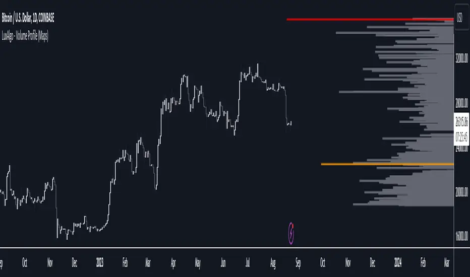
Volume Profile (Maps) [LuxAlgo]The Pine Script® developers have unleashed "maps"!
Volume Profile (Maps) displays volume, associated with price, above and below the latest price, by using maps
The largest and second-largest volume is highlighted.
🔶 USAGE
The proposed script can highlight more frequent closing prices/prices with the highest volume, potentially highlighting more liquid areas. The prices with the highest associated volume (in red and orange in the indicator) can eventually be used as support/resistance levels.
Voids within the volume profile can highlight large price displacements (volatile variations).
🔶 CONCEPTS
🔹 Maps
A map object is a collection that consists of key - value pairs
Each key is unique and can only appear once. When adding a new value with a key that the map already contains, that value replaces the old value associated with the key .
You can change the value of a particular key though, for example adding volume (value) at the same price (key), the latter technique is used in this script.
Volume is added to the map, associated with a particular price (default close, can be set at high, low, open,...)
When the map already contains the same price (key), the value (volume) is added to the existing volume at the associated price.
A map can contain maximum 50K values, which is more than enough to hold 20K bars (Basic 5K - Premium plan 20K), so the whole history can be put into a map.
🔹 Visible line/box limit
We can only display maximum 500 line.new() though.
The code locates the current (last) close, and displays volume values around this price, using lines, for example 250 lines above and 250 lines below current price.
If one side contains fewer values, the other side can show more lines, taking the maximum out of the 500 visible line limitation.
Example (max. 500 lines visible)
• 100 values below close
• 2000 values above close
-> 100 values will be displayed below close
-> 400 remaining -> 400 values will be displayed above close
Pushing the limits even further, when ' Amount of bars ' is set higher than 500, boxes - box.new() - will be used as well.
These have a limit of 500 as well, bringing the total limit to 1000.
Note that there are visual differences when boxes overlap against lines.
If this is confusing, please keep ' Amount of bars ' at max. 500 (then only lines will be used).
🔹 Rounding function
This publication contains 2 round functions, which can be used to widen the Volume Profile
Round
• "Round" set at zero -> nothing changes to the source number
• "Round" set below zero -> x digit(s) after the decimal point, starting from the right side, and rounded.
• "Round" set above zero -> x digit(s) before the decimal point, starting from the right side, and rounded.
Example: 123456.789
0->123456.789
1->123456.79
2->123456.8
3->123457
-1->123460
-2->123500
Step
Another option is custom steps.
After setting "Round" to "Step", choose the desired steps in price,
Examples
• 2 -> 1234.00, 1236.00, 1238.00, 1240.00
• 5 -> 1230.00, 1235.00, 1240.00, 1245.00
• 100 -> 1200.00, 1300.00, 1400.00, 1500.00
• 0.05 -> 1234.00, 1234.05, 1234.10, 1234.15
•••
🔶 FEATURES
🔹 Adjust position & width
🔹 Table
The table shows the details:
• Size originalMap : amount of elements in original map
• # higher: amount of elements, higher than last "close" (source)
• index "close" : index of last "close" (source), or # element, lower than source
• Size newMap : amount of elements in new map (used for display lines)
• # higher : amount of elements in newMap, higher than last "close" (source)
• # lower : amount of elements in newMap, lower than last "close" (source)
🔹 Volume * currency
Let's take as example BTCUSD, relative to USD, 10 volume at a price of 100 BTCUSD will be very different than 10 volume at a price of 30000 (1K vs. 300K)
If you want volume to be associated with USD, enable Volume * currency . Volume will then be multiplied by the price:
• 10 volume, 1 BTC = 100 -> 1000
• 10 volume, 1 BTC = 30K -> 300K
Disabled
Enabled
🔶 DETAILS
🔹 Put
When the map doesn't contain a price, it will be added, using map.put(id, key, value)
In our code:
map.put(originalMap, price, volume)
or
originalMap.put(price, volume)
A key (price) is now associated with a value (volume) -> key : value
Since all keys are unique, we don't have to know its position to extract the value, we just need to know the key -> map.get(id, key)
We use map.get() when a certain key already exists in the map, and we want to add volume with that value.
if originalMap.contains(price)
originalMap.put(price, originalMap.get(price) + volume)
-> At the last bar, all prices (source) are now associated with volume.
🔹 Copy & sort
Next, every key of the map is copied and sorted (array of keys), after which the index (idx) is retrieved of last (current) price.
copyK = originalMap.keys().copy()
copyK.sort()
idx = copyK.binary_search_leftmost(src)
Then left and right side of idx is investigated to show a maximum amount of lines at both sides of last price.
🔹 New map & display
The keys (from sorted array of copied keys) that will be displayed are put in a new map, with the associated volume values from the original map.
newMap = map.new()
🔹 Re-cap
• put in original amp (price key, volume value)
• copy & sort
• find index of last price
• fetch relevant keys left/right from that index
• put keys in new map and fetch volume associated with these keys (from original map)
Simple example (only show 5 lines)
bar 0, price = 2, volume = 23
bar 1, price = 4, volume = 3
bar 2, price = 8, volume = 21
bar 3, price = 6, volume = 7
bar 4, price = 9, volume = 13
bar 5, price = 5, volume = 85
bar 6, price = 3, volume = 13
bar 7, price = 1, volume = 4
bar 8, price = 7, volume = 9
Original map:
Copied keys array:
Sorted:
-> 5 keys around last price (7) are fetched (5, 6, 7, 8, 9)
-> keys are placed into new map + volume values from original map
Lastly, these values are displayed.
🔶 SETTINGS
Source : Set source of choice; default close , can be set as high , low , open , ...
Volume & currency : Enable to multiply volume with price (see Features )
Amount of bars : Set amount of bars which you want to include in the Volume Profile
Max lines : maximum 1000 (if you want to use only lines, and no boxes -> max. 500, see Concepts )
🔹 Round -> ' Round/Step '
Round -> see Concepts
Step -> see Concepts
🔹 Display Volume Profile
Offset: shifts the Volume Profile (max. 500 bars to the right of last bar, see Features )
Max width Volume Profile: largest volume will be x bars wide, the rest is displayed as a ratio against largest volume (see Features )
Show table : Show details (see Features )
🔶 LIMITATIONS
• Lines won't go further than first bar (coded).
• The Volume Profile can be placed maximum 500 bar to the right of last price.
• Maximum 500 lines/boxes can be displayed
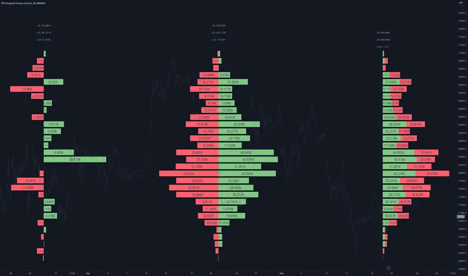
Open Interest Profile [Fixed Range] - By LeviathanThis script generates an aggregated Open Interest profile for any user-selected range and provides several other features and tools, such as OI Delta Profile, Positive Delta Levels, OI Heatmap, Range Levels, OIWAP, POC and much more.
The indicator will help you find levels of interest based on where other market participants are opening and closing their positions. This provides a deeper insight into market activity and serves as a foundation for various different trading strategies (trapped traders, supply and demand, support and resistance, liquidity gaps, imbalances,liquidation levels, etc). Additionally, this indicator can be used in conjunction with other tools such as Volume Profile.
Open Interest (OI) is a key metric in derivatives markets that refers to the total number of unsettled or open contracts. A contract is a mutual agreement between two parties to buy or sell an underlying asset at a predetermined price. Each contract consists of a long side and a short side, with one party consenting to buy (long) and the other agreeing to sell (short). The party holding the long position will profit from an increase in the asset's price, while the one holding the short position will profit from the price decline. Every long position opened requires a corresponding short position by another market participant, and vice versa. Although there might be an imbalance in the number of accounts or traders holding long and short contracts, the net value of positions held on each side remains balanced at a 1:1 ratio. For instance, an Open Interest of 100 BTC implies that there are currently 100 BTC worth of longs and 100 BTC worth of shorts open in the market. There might be more traders on one side holding smaller positions, and fewer on the other side with larger positions, but the net value of positions on both sides is equivalent - 100 BTC in longs and 100 BTC in shorts (1:1). Consider a scenario where a trader decides to open a long position for 1 BTC at a price of $30k. For this long order to be executed, a counterparty must take the opposite side of the contract by placing a short order for 1 BTC at the same price of $30k. When both long and short orders are matched and executed, the Open Interest increases by 1 BTC, indicating the introduction of this new contract to the market.
The meaning of fluctuations in Open Interest:
- OI Increase - signifies new positions entering the market (both longs and shorts).
- OI Decrease - indicates positions exiting the market (both longs and shorts).
- OI Flat - represents no change in open positions due to low activity or a large number of contract transfers (contracts changing hands instead of being closed).
Typically, we monitor Open Interest in the form of its running value, either on a chart or through OI Delta histograms that depict the net change in OI for each price bar. This indicator enhances Open Interest analysis by illustrating the distribution of changes in OI on the price axis rather than the time axis (akin to Volume Profiles). While Volume Profile displays the volume that occurred at a given price level, the Open Interest Profile offers insight into where traders were opening and closing their positions.
How to use the indicator?
1. Add the script to your chart
2. A prompt will appear, asking you to select the “Start Time” (start of the range) and the “End Time” (end of the range) by clicking anywhere on your chart.
3. Within a few seconds, a profile will be generated. If you wish to alter the selected range, you can drag the "Start Time" and "End Time" markers accordingly.
4. Enjoy the script and feel free to explore all the settings.
To learn more about each input in indicator settings, please read the provided tooltips. These can be accessed by hovering over or clicking on the ( i ) symbol next to the input.
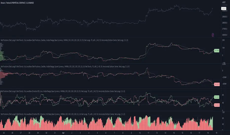
Net Positions (Net Longs & Net Shorts) - By LeviathanThis script is an experimental indicator that visualizes the entering and exiting of long and short positions in the market. It also includes other useful tools, such as NL/NS Profile, NL/NS Delta, NL/NS Ratio, Volume Heatmap, Divergence finder, Relative Strength Index of Net Longs and Net Shorts, EMAs and VWMAs and more.
To avoid misinterpretation, it's important to understand some basics. The “real” ratio between net long and net short positions in a given market is always 1:1. A futures contract is an agreement between two parties to buy or sell an underlying asset at an agreed-upon price. Each contract has a long side and a short side, with one party agreeing to buy (long) and the other party agreeing to sell (short) the asset at the agreed-upon price. The long position holder anticipates that the asset's price will rise, while the short position holder expects it to fall. Because every futures contract involves both a buyer and a seller, it is impossible to have more net longs than net shorts or vice versa (in terms of the net value). For every long position opened, there must be a corresponding short position taken by another market participant (and vice versa), thus maintaining the 1:1 ratio between longs and shorts. While there can be an imbalance in the number of traders/accounts holding long and short contracts, the net value of positions held on each side remains 1 to 1.
Open Interest (OI) is a metric that tracks the number of open (unsettled) contracts in a given market. For example, Open Interest of 100 BTC means that there are currently 100 BTC worth of longs and 100 BTC worth of shorts open in the market. There may be more traders on one side holding smaller positions, and fewer traders on the other side holding larger positions, but the net value of positions on one side is equal to the net value of positions on the other side → 100 BTC in longs and 100 BTC in shorts (1:1). Consider a scenario in which a trader decides to open a long position for 1 BTC at a price of HKEX:30 ,000. For this long order to be executed, a counterparty must take the opposite side of the contract by placing an order to short 1 BTC at the same price of HKEX:30 ,000. When both the long and short orders are matched and executed, the open interest increases by 1 BTC, reflecting the addition of this new contract to the market.
Changes in Open Interest essentially tell us 3 things:
- OI Increase - new positions entered the market (both longs and shorts!)
- OI Decrease - positions exited the market (both longs and shorts!)
- OI Flat - no change in open positions due to low activity or simply lots of transfers of contracts
However, different concepts can be used to analyze sentiment, aggressiveness, and activity in the market by analyzing data such as Open Interest, price, volume, etc. This indicator combines Open Interest data and price action to simplify the visualization of positions entering and exiting the market. It is based on the following concept:
Increase in Open Interest + Increase in price = Longs Opening
Decrease in Open Interest + Decrease in price = Longs Closing
Increase in Open Interest + Decrease in price = Shorts Opening
Decrease in Open Interest + Increase in price = Shorts Closing
When "Longs Opening" occurs, the OI Delta value is added to the running total of Net Longs, and when "Longs Closing" occurs, the OI Delta value is subtracted from the running total of Net Longs.
When "Shorts Opening" occurs, the OI Delta value is added to the running total of Net Shorts, and when "Shorts Closing" occurs, the OI Delta value is subtracted from the running total of Net Shorts.
To summarize:
Net Longs: Cumulative value of Longs Opening and Longs Closing (LO - LC)
Net Shorts: Cumulative value of Shorts Opening and Shorts Closing (SO - SC)
Net Delta: Net Longs - Net Shorts
Net Ratio: Net Longs / Net Shorts
This is the fundamental logic of how this script functions, but it also includes several other tools and options. Here is an overview of the settings:
Type:
- Net Positions (display values of Net Longs, Net Shorts, Net Delta, Net Ratio as described above)
- Relative Strength (display Net Longs, Net Shorts, Net Delta, Net Ratio in the form of a momentum oscillator that measures the speed and change of movements. Same logic as RSI for price)
Display as:
- Candles (display the data in the form of candlesticks)
- Lines (display the data in the form of candlesticks)
- Columns (display the data in the form of columns)
Cumulation:
- Visible Range (data is cumulated from the first visible bar on your chart)
- Full Data (data is cumulated from the beginning)
Quoted in:
- Base Currency (all data is presented in the pair’s base currency eg. BTC)
- Quote Currency (all data is presented in the pair’s quote currency eg USDT)
OI Sources
- Pick the sources from where the data is collected (if available).
Net Positions:
- NET LONGS (show/hide Net Longs plot, choose candle colors, choose line color)
- NET SHORTS (show/hide Net Shorts plot, choose candle colors, choose line color)
- NET DELTA (show/hide Net Delta plot, choose candle colors, choose line color)
- NET RATIO (show/hide Net Ratio plot, choose candle colors, choose line color)
Moving Averages:
- Type (choose between EMA and Volume Weighted Moving Average)
- NET LONGS (show/hide NL moving average plot, choose length, choose color)
- NET SHORTS (show/hide NS moving average plot, choose length, choose color)
- NET DELTA (show/hide ND moving average plot, choose length, choose color)
- NET RATIO (show/hide NR moving average plot, choose length, choose color)
Profile:
- Profile Data (choose the source data of the profile)
- Value Area % (set the percentage width of profile’s value area)
- Positions (set the position of the profile to left or right of the visible range)
- Node Size (set the relative size of nodes to make them appear smaller or larger)
- Rows (select the amount of rows displayed by the profile to control granularity)
- POC (show/hide POC- Point Of Control and select its color)
- VA (show/hide VA- Value Area and select its color)
Divergence finder
- Source (choose the source data used by the script to compare it with price pivot points)
- Maximum distance (the maximum distance between two divergent pivot points)
- Lookback Bars Left (the number of bars to the left of the current bar that the function will consider when looking for a pivot point)
- Lookback Bars Right (the number of bars to the right of the current bar that the function will consider when looking for a pivot point)
Stats:
- Show/Hide the Stats table
- Bars Back (choose the length of data analyzed for stats in number of bars)
- Position (choose the position of the Stats table)
- Select Data you want to display in the Stats table
Additional Settings:
- Volume Heatmap (show/hide volume heatmap and select its color)
- Label Offset (select how much the plot label is shifted to the right
- Position Relative Strength Length (select the length used in the calculation)
- Value Label (show/hide OI Delta values when candles are displayed)
- Plot Labels (show/hide the labels next to the plot)
- Wicks (show/hide wick when candles are displayed)
Code used for generating profiles is taken from @KioseffTrading's "Profile Any Indicator" script (used with author's permission)
Wavemeter [theEccentricTrader]█ OVERVIEW
This indicator is a representation of my take on price action based wave cycle theory. The indicator counts the number of confirmed wave cycles, keeps a rolling tally of the average wave length, wave height and frequency, and displays the statistics in a table. The indicator also displays the current wave measurements as an optional feature.
█ CONCEPTS
Green and Red Candles
• A green candle is one that closes with a high price equal to or above the price it opened.
• A red candle is one that closes with a low price that is lower than the price it opened.
Swing Highs and Swing Lows
• A swing high is a green candle or series of consecutive green candles followed by a single red candle to complete the swing and form the peak.
• A swing low is a red candle or series of consecutive red candles followed by a single green candle to complete the swing and form the trough.
Peak and Trough Prices (Basic)
• The peak price of a complete swing high is the high price of either the red candle that completes the swing high or the high price of the preceding green candle, depending on which is higher.
• The trough price of a complete swing low is the low price of either the green candle that completes the swing low or the low price of the preceding red candle, depending on which is lower.
Historic Peaks and Troughs
The current, or most recent, peak and trough occurrences are referred to as occurrence zero. Previous peak and trough occurrences are referred to as historic and ordered numerically from right to left, with the most recent historic peak and trough occurrences being occurrence one.
Wave Cycles
A wave cycle is here defined as a complete two-part move between a swing high and a swing low, or a swing low and a swing high. As can be seen in the example above, the first swing high or swing low will set the course for the sequence of wave cycles that follow; a chart that begins with a swing low will form its first complete wave cycle upon the formation of the first complete swing high and vice versa.
Wave Length
Wave length is here measured in terms of bar distance between the start and end of a wave cycle. For example, if the current wave cycle ends on a swing low the wave length will be the difference in bars between the current swing low and current swing high. In such a case, if the current swing low completes on candle 100 and the current swing high completed on candle 95, we would simply subtract 95 from 100 to give us a wave length of 5 bars.
Average wave length is here measured in terms of total bars as a proportion as total waves. The average wavelength is calculated by dividing the total candles by the total wave cycles.
Wave Height
Wave height is here measured in terms of current range. For example, if the current peak price is 100 and the current trough price is 80, the wave height will be 20.
Amplitude
Amplitude is here measured in terms of current range divided by two. For example if the current peak price is 100 and the current trough price is 80, the amplitude would be calculated by subtracting 80 from 100 and dividing the answer by 2 to give us an amplitude of 10.
Frequency
Frequency is here measured in terms of wave cycles per second (Hertz). For example, if the total wave cycle count is 10 and the amount of time it has taken to complete these 10 cycles is 1-year (31,536,000 seconds), the frequency would be calculated by dividing 10 by 31,536,000 to give us a frequency of 0.00000032 Hz.
Range
The range is simply the difference between the current peak and current trough prices, generally expressed in terms of points or pips.
█ FEATURES
Inputs
Show Sample Period
Start Date
End Date
Position
Text Size
Show Current
Show Lines
Table
The table is colour coded, consists of two columns and, as many as, nine rows. Blue cells display the total wave cycle count and average wave measurements. Green cells display the current wave measurements. And the final row in column one, coloured black, displays the sample period. Both current wave measurements and sample period cells can be hidden at the user’s discretion.
Lines
For a visual aid to the wave cycles, I have added a blue line that traces out the waves on the chart. These lines can be hidden at the user’s discretion.
█ HOW TO USE
The indicator is intended for research purposes, strategy development and strategy optimisation. I hope it will be useful in helping to gain a better understanding of the underlying dynamics at play on any given market and timeframe.
For example, the indicator can be used to compare the current range and frequency with the average range and frequency, which can be useful for gauging current market conditions versus historic and getting a feel for how different markets and timeframes behave.
█ LIMITATIONS
Some higher timeframe candles on tickers with larger lookbacks such as the DXY , do not actually contain all the open, high, low and close (OHLC) data at the beginning of the chart. Instead, they use the close price for open, high and low prices. So, while we can determine whether the close price is higher or lower than the preceding close price, there is no way of knowing what actually happened intra-bar for these candles. And by default candles that close at the same price as the open price, will be counted as green. You can avoid this problem by utilising the sample period filter.
The green and red candle calculations are based solely on differences between open and close prices, as such I have made no attempt to account for green candles that gap lower and close below the close price of the preceding candle, or red candles that gap higher and close above the close price of the preceding candle. I can only recommend using 24-hour markets, if and where possible, as there are far fewer gaps and, generally, more data to work with. Alternatively, you can replace the scenarios with your own logic to account for the gap anomalies, if you are feeling up to the challenge.
It is also worth noting that the sample size will be limited to your Trading View subscription plan. Premium users get 20,000 candles worth of data, pro+ and pro users get 10,000, and basic users get 5,000. If upgrading is currently not an option, you can always keep a rolling tally of the statistics in an excel spreadsheet or something of the like.

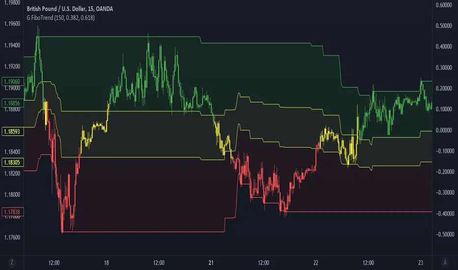
Gedhusek TrendFibonacciThis indicator is a trend filter based on fibonacci retracement levels
How to read:
- There are three filled zones --> red, yellow and green
- If the price is inside of red zone, there is a downtrend on the market
- If the price is inside the yellow zone, there is a sideways trend on the market
- If the price is inside the green zone, there is a uptrend on the market
- Also, candles are going to have a corresponding color based on the current trend
Calculations of the indicator:
1. Calculate distance between maximal and minimal price over the last "x" bars (choose value for "x" in inputs menu under the "Analysis period")
2. Use this distance for calculating two retracement levels (choose retracement levels in inputs menu)
3. These two retracement levels create an area of what is going to be considered as sideways market
Example:
- Lets say we chose Analysis period of 100, Lower Fibonacci Level as 0.382 and Upper Fibonacci Level as 0.618
- Maximum price over the last 100 bars was of 120 and minimum price was 20. That leaves us with the difference of 100 points
- Now we calculate the fibonacci levels --> 100*0.382 = 38.2 and 100*0.618 = 61.8
- The next step is to add the levels to the lowest price point --> 20 + 38.2 = 58.2 and 20 + 61.8 = 81.8
- And now we have our zones. If the price is going to be below the lower fibonacci level (in this case 58.2), we consider it as a bearish trend. If the price is between those fibonacci levels (58.2 and 81.8), we consider it as a sideways trend. And if the price is above the upper fibonacci level (81.8), we consider it as a bullish trend.
Inputs:
- Analysis period --> number of bars within which the system is going to look for max and min price
- Lower Fibonacci Level --> Choose from options and must be lower or the same as "Upper Fibonacci Level"
- Upper Fibonacci Level --> Choose from options and must be higher or the same as "Lower Fibonacci Level"
- Show Filling --> whether you wish to fill the areas with color
- Change Candle Color --> whether you wish to change the color of candles based on current trend.
Volatility Risk Premium (VRP) 1.0ENGLISH
This indicator (V-R-P) calculates the (one month) Volatility Risk Premium for S&P500 and Nasdaq-100.
V-R-P is the premium hedgers pay for over Realized Volatility for S&P500 and Nasdaq-100 index options.
The premium stems from hedgers paying to insure their portfolios, and manifests itself in the differential between the price at which options are sold (Implied Volatility) and the volatility the S&P500 and Nasdaq-100 ultimately realize (Realized Volatility).
I am using 30-day Implied Volatility (IV) and 21-day Realized Volatility (HV) as the basis for my calculation, as one month of IV is based on 30 calendaristic days and one month of HV is based on 21 trading days.
At first, the indicator appears blank and a label instructs you to choose which index you want the V-R-P to plot on the chart. Use the indicator settings (the sprocket) to choose one of the indices (or both).
Together with the V-R-P line, the indicator will show its one year moving average within a range of +/- 15% (which you can change) for benchmarking purposes. We should consider this range the “normalized” V-R-P for the actual period.
The Zero Line is also marked on the indicator.
Interpretation
When V-R-P is within the “normalized” range, … well... volatility and uncertainty, as it’s seen by the option market, is “normal”. We have a “premium” of volatility which should be considered normal.
When V-R-P is above the “normalized” range, the volatility premium is high. This means that investors are willing to pay more for options because they see an increasing uncertainty in markets.
When V-R-P is below the “normalized” range but positive (above the Zero line), the premium investors are willing to pay for risk is low, meaning they see decreasing uncertainty and risks in the market, but not by much.
When V-R-P is negative (below the Zero line), we have COMPLACENCY. This means investors see upcoming risk as being lower than what happened in the market in the recent past (within the last 30 days).
CONCEPTS:
Volatility Risk Premium
The volatility risk premium (V-R-P) is the notion that implied volatility (IV) tends to be higher than realized volatility (HV) as market participants tend to overestimate the likelihood of a significant market crash.
This overestimation may account for an increase in demand for options as protection against an equity portfolio. Basically, this heightened perception of risk may lead to a higher willingness to pay for these options to hedge a portfolio.
In other words, investors are willing to pay a premium for options to have protection against significant market crashes even if statistically the probability of these crashes is lesser or even negligible.
Therefore, the tendency of implied volatility is to be higher than realized volatility, thus V-R-P being positive.
Realized/Historical Volatility
Historical Volatility (HV) is the statistical measure of the dispersion of returns for an index over a given period of time.
Historical volatility is a well-known concept in finance, but there is confusion in how exactly it is calculated. Different sources may use slightly different historical volatility formulas.
For calculating Historical Volatility I am using the most common approach: annualized standard deviation of logarithmic returns, based on daily closing prices.
Implied Volatility
Implied Volatility (IV) is the market's forecast of a likely movement in the price of the index and it is expressed annualized, using percentages and standard deviations over a specified time horizon (usually 30 days).
IV is used to price options contracts where high implied volatility results in options with higher premiums and vice versa. Also, options supply and demand and time value are major determining factors for calculating Implied Volatility.
Implied Volatility usually increases in bearish markets and decreases when the market is bullish.
For determining S&P500 and Nasdaq-100 implied volatility I used their volatility indices: VIX and VXN (30-day IV) provided by CBOE.
Warning
Please be aware that because CBOE doesn’t provide real-time data in Tradingview, my V-R-P calculation is also delayed, so you shouldn’t use it in the first 15 minutes after the opening.
This indicator is calibrated for a daily time frame.
ESPAŇOL
Este indicador (V-R-P) calcula la Prima de Riesgo de Volatilidad (de un mes) para S&P500 y Nasdaq-100.
V-R-P es la prima que pagan los hedgers sobre la Volatilidad Realizada para las opciones de los índices S&P500 y Nasdaq-100.
La prima proviene de los hedgers que pagan para asegurar sus carteras y se manifiesta en el diferencial entre el precio al que se venden las opciones (Volatilidad Implícita) y la volatilidad que finalmente se realiza en el S&P500 y el Nasdaq-100 (Volatilidad Realizada).
Estoy utilizando la Volatilidad Implícita (IV) de 30 días y la Volatilidad Realizada (HV) de 21 días como base para mi cálculo, ya que un mes de IV se basa en 30 días calendario y un mes de HV se basa en 21 días de negociación.
Al principio, el indicador aparece en blanco y una etiqueta le indica que elija qué índice desea que el V-R-P represente en el gráfico. Use la configuración del indicador (la rueda dentada) para elegir uno de los índices (o ambos).
Junto con la línea V-R-P, el indicador mostrará su promedio móvil de un año dentro de un rango de +/- 15% (que puede cambiar) con fines de evaluación comparativa. Deberíamos considerar este rango como el V-R-P "normalizado" para el período real.
La línea Cero también está marcada en el indicador.
Interpretación
Cuando el V-R-P está dentro del rango "normalizado",... bueno... la volatilidad y la incertidumbre, como las ve el mercado de opciones, es "normal". Tenemos una “prima” de volatilidad que debería considerarse normal.
Cuando V-R-P está por encima del rango "normalizado", la prima de volatilidad es alta. Esto significa que los inversores están dispuestos a pagar más por las opciones porque ven una creciente incertidumbre en los mercados.
Cuando el V-R-P está por debajo del rango "normalizado" pero es positivo (por encima de la línea Cero), la prima que los inversores están dispuestos a pagar por el riesgo es baja, lo que significa que ven una disminución, pero no pronunciada, de la incertidumbre y los riesgos en el mercado.
Cuando V-R-P es negativo (por debajo de la línea Cero), tenemos COMPLACENCIA. Esto significa que los inversores ven el riesgo próximo como menor que lo que sucedió en el mercado en el pasado reciente (en los últimos 30 días).
CONCEPTOS:
Prima de Riesgo de Volatilidad
La Prima de Riesgo de Volatilidad (V-R-P) es la noción de que la Volatilidad Implícita (IV) tiende a ser más alta que la Volatilidad Realizada (HV) ya que los participantes del mercado tienden a sobrestimar la probabilidad de una caída significativa del mercado.
Esta sobreestimación puede explicar un aumento en la demanda de opciones como protección contra una cartera de acciones. Básicamente, esta mayor percepción de riesgo puede conducir a una mayor disposición a pagar por estas opciones para cubrir una cartera.
En otras palabras, los inversores están dispuestos a pagar una prima por las opciones para tener protección contra caídas significativas del mercado, incluso si estadísticamente la probabilidad de estas caídas es menor o insignificante.
Por lo tanto, la tendencia de la Volatilidad Implícita es de ser mayor que la Volatilidad Realizada, por lo cual el V-R-P es positivo.
Volatilidad Realizada/Histórica
La Volatilidad Histórica (HV) es la medida estadística de la dispersión de los rendimientos de un índice durante un período de tiempo determinado.
La Volatilidad Histórica es un concepto bien conocido en finanzas, pero existe confusión sobre cómo se calcula exactamente. Varias fuentes pueden usar fórmulas de Volatilidad Histórica ligeramente diferentes.
Para calcular la Volatilidad Histórica, utilicé el enfoque más común: desviación estándar anualizada de rendimientos logarítmicos, basada en los precios de cierre diarios.
Volatilidad Implícita
La Volatilidad Implícita (IV) es la previsión del mercado de un posible movimiento en el precio del índice y se expresa anualizada, utilizando porcentajes y desviaciones estándar en un horizonte de tiempo específico (generalmente 30 días).
IV se utiliza para cotizar contratos de opciones donde la alta Volatilidad Implícita da como resultado opciones con primas más altas y viceversa. Además, la oferta y la demanda de opciones y el valor temporal son factores determinantes importantes para calcular la Volatilidad Implícita.
La Volatilidad Implícita generalmente aumenta en los mercados bajistas y disminuye cuando el mercado es alcista.
Para determinar la Volatilidad Implícita de S&P500 y Nasdaq-100 utilicé sus índices de volatilidad: VIX y VXN (30 días IV) proporcionados por CBOE.
Precaución
Tenga en cuenta que debido a que CBOE no proporciona datos en tiempo real en Tradingview, mi cálculo de V-R-P también se retrasa, y por este motivo no se recomienda usar en los primeros 15 minutos desde la apertura.
Este indicador está calibrado para un marco de tiempo diario.
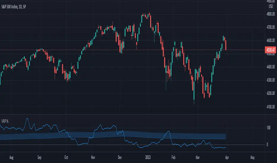
Drawdown + Labels BINANCE:BTCUSDT
Indicador de reducciones de precio con etiqueta.
El indicador toma por defecto el valor máximo histórico y a partir de ese valor realiza los siguientes cálculos:
Reducción del 50% = Máximo Histórico*(50/100)
Reducción del 60% = Máximo Histórico*(40/100)
Reducción del 70% = Máximo Histórico*(30/100)
Reducción del 80% = Máximo Histórico*(20/100)
Reducción del 90% = Máximo Histórico*(10/100)
En el grafico se mostrará una etiqueta a la derecha por defecto, el valor que corresponde a cada reducción.
Ejemplo:
Fecha: 04 de Enero de 2022
Máximo Histórico de BTC = $ 69,000 (Línea color Naranja)
Reducción del 50% = $ 34,500 (Línea color Morada)
Reducción del 60% = $ 27,600 (Línea color Marrón)
Reducción del 70% = $ 20,700 (Línea color Verde)
Reducción del 80% = $ 13,800 (Línea color Roja)
Reducción del 90% = $ 6,900 (Línea color Aqua)
Reducción del 100% = $ 0 (Línea color Negro)
Espero les ayude, saludos.

Portfolio Backtester Engine█ OVERVIEW
Portfolio Backtester Engine (PBTE). This tool will allow you to backtest strategies across multiple securities at once. Allowing you to easier understand if your strategy is robust. If you are familiar with the PineCoders backtesting engine , then you will find this indicator pleasant to work with as it is an adaptation based on that work. Much of the functionality has been kept the same, or enhanced, with some minor adjustments I made on the account of creating a more subjectively intuitive tool.
█ HISTORY
The original purpose of the backtesting engine (`BTE`) was to bridge the gap between strategies and studies . Previously, strategies did not contain the ability to send alerts, but were necessary for backtesting. Studies on the other hand were necessary for sending alerts, but could not provide backtesting results . Often, traders would have to manage two separate Pine scripts to take advantage of each feature, this was less than ideal.
The `BTE` published by PineCoders offered a solution to this issue by generating backtesting results under the context of a study(). This allowed traders to backtest their strategy and simultaneously generate alerts for automated trading, thus eliminating the need for a separate strategy() script (though, even converting the engine to a strategy was made simple by the PineCoders!).
Fast forward a couple years and PineScript evolved beyond these issues and alerts were introduced into strategies. The BTE was not quite as necessary anymore, but is still extremely useful as it contains extra features and data not found under the strategy() context. Below is an excerpt of features contained by the BTE:
"""
More than `40` built-in strategies,
Customizable components,
Coupling with your own external indicator,
Simple conversion from Study to Strategy modes,
Post-Exit analysis to search for alternate trade outcomes,
Use of the Data Window to show detailed bar by bar trade information and global statistics, including some not provided by TV backtesting,
Plotting of reminders and generation of alerts on in-trade events.
"""
Before I go any further, I want to be clear that the BTE is STILL a good tool and it is STILL very useful. The Portfolio Backtesting Engine I am introducing is only a tangental advancement and not to be confused as a replacement, this tool would not have been possible without the `BTE`.
█ THE PROBLEM
Most strategies built in Pine are limited by one thing. Data. Backtesting should be a rigorous process and researchers should examine the performance of their strategy across all market regimes; that includes, bullish and bearish markets, ranging markets, low volatility and high volatility. Depending on your TV subscription The Pine Engine is limited to 5k-20k historical bars available for backtesting, which can often leave the strategy results wanting. As a general rule of thumb, strategies should be tested across a quantity of historical bars which will allow for at least 100 trades. In many cases, the lack of historical bars available for backtesting and frequency of the strategy signals produces less than 100 trades, rendering your strategy results inconclusive.
█ THE SOLUTION
In order to be confident that we have a robust strategy we must test it across all market regimes and we must have over 100 trades. To do this effectively, researchers can use the Portfolio Backtesting Engine (PBTE).
By testing a strategy across a carefully selected portfolio of securities, researchers can now gather 5k-20k historical bars per security! Currently, the PTBE allows up to 5 securities, which amounts to 25k-100k historical bars.
█ HOW TO USE
1 — Add the indicator to your chart.
• Confirm inputs. These will be the most important initial values which you can change later by clicking the gear icon ⚙ and opening up the settings of the indicator.
2 — Select a portfolio.
• You will want to spend some time carefully selecting a portfolio of securities.
• Each security should be uncorrelated.
• The entire portfolio should contain a mix of different market regimes.
You should understand that strategies generally take advantage of one particular type of market regime. (trending, ranging, low/high volatility)
For example, the default RSI strategy is typically advantageous during ranging markets, whereas a typical moving average crossover strategy is advantageous in trending markets.
If you were to use the standard RSI strategy during a trending market, you might be selling when you should be buying.
Similarily, if you use an SMA crossover during a ranging market, you will find that the MA's may produce many false signals.
Even if you build a strategy that is designed to be used only in a trending market, it is still best to select a portfolio of all market regimes
as you will be able to test how your strategy will perform when the market does something unexpected.
3 — Test a built-in strategy or add your own.
• Navigate to gear icon ⚙ (settings) of strategy.
• Choose your options.
• Select a Main Entry Strat and Alternate Entry Strat .
• If you want to add your own strategy, you will need to modify the source code and follow the built-in example.
• You will only need to generate (buy 1 / sell -1/ neutral 0) signals.
• Select a Filter , by default these are all off.
• Select an Entry Stop - This will be your stop loss placed at the trade entry.
• Select Pyamiding - This will allow you to stack positions. By default this is off.
• Select Hard Exits - You can also think of these as Take Profits.
• Let the strategy run and take note of the display tables results.
• Portfolio - Shows each security.
• The strategy runs on each asset in your portfolio.
• The initial capital is equally distributed across each security.
So if you have 5 securities and a starting capital of 100,000$ then each security will run the strategy starting with 20,000$
The total row will aggregate the results on a bar by bar basis showing the total results of your initial capital.
• Net Profit (NP) - Shows profitability.
• Number of Trades (#T) - Shows # of trades taken during backtesting period.
• Typically will want to see this number greater than 100 on the "Total" row.
• Average Trade Length (ATL) - Shows average # of days in a trade.
• Maximum Drawdown (MD ) - Max peak-to-valley equity drawdown during backtesting period.
• This number defines the minimum amount of capital required to trade the system.
• Typically, this shouldn’t be lower than 34% and we will want to allow for at least 50% beyond this number.
• Maximum Loss (ML) - Shows largest loss experienced on a per-trade basis.
• Normally, don’t want to exceed more than 1-2 % of equity.
• Maximum Drawdown Duration (MDD) - The longest duration of a drawdown in equity prior to a new equity peak.
• This number is important to help us psychologically understand how long we can expect to wait for a new peak in account equity.
• Maximum Consecutive Losses (MCL) - The max consecutive losses endured throughout the backtesting period.
• Another important metric for trader psychology, this will help you understand how many losses you should be prepared to handle.
• Profit to Maximum Drawdown (P:MD) - A ratio for the average profit to the maximum drawdown.
• The higher the ratio is, the better. Large profits and small losses contribute to a good PMD.
• This metric allows us to examine the profit with respect to risk.
• Profit Loss Ratio (P:L) - Average profit over the average loss.
• Typically this number should be higher in trend following systems.
• Mean reversion systems show lower values, but compensate with a better win %.
• Percent Winners (% W) - The percentage of winning trades.
• Trend systems will usually have lower win percentages, since statistically the market is only trending roughly 30% of the time.
• Mean reversion systems typically should have a high % W.
• Time Percentage (Time %) - The amount of time that the system has an open position.
• The more time you are in the market, the more you are exposed to market risk, not to mention you could be using that money for something else right?
• Return on Investment (ROI) - Your Net Profit over your initial investment, represented as a percentage.
• You want this number to be positive and high.
• Open Profit (OP) - If the strategy has any open positions, the floating value will be represented here.
• Trading Days (TD) - An important metric showing how many days the strategy was active.
• This is good to know and will be valuable in understanding how long you will need to run this strategy in order to achieve results.
█ FEATURES
These are additional features that extend the original `BTE` features.
- Portfolio backtesting.
- Color coded performance results.
- Circuit Breakers that will stop trading.
- Position reversals on exit. (Simulating the function of always in the market. Similar to strategy.entry functionality)
- Whipsaw Filter
- Moving Average Filter
- Minimum Change Filter
- % Gain Equity Exit
- Popular strategies, (MACD, MA cross, supertrend)
Below are features that were excluded from the original `BTE`
- 2 stage in-trade stops with kick-in rules (This was a subjective decision to remove. I found it to be complex and thwarted my use of the `BTE` for some time.)
- Simple conversion from Study to Strategy modes. (Not possible with multiple securities)
- Coupling with your own external indicator (Not really practical to use with multiple securities, but could be used if signals were generated based on some indicator which was not based on the current chart)
- Use of the Data Window to show detailed bar by bar trade information and global statistics.
- Post Exit Analysis.
- Plotting of reminders and generation of alerts on in-trade events.
- Alerts (These may be added in the future by request when I find the time.)
█ THANKS
The whole PineCoders team for all their shared knowledge and original publication of the BTE and Richard Weismann for his ideas on building robust strategies.
═════════════════════════════════════════════════════════════════════════

Fixed price Stop Loss [Takazudo]This strategy is a demo for fixed price stop loss.
This strategy enables you to specify fixed price stop loss. Let's say your deposit is USD. When you trade EURCAD, you need to specify the quantity for trade. Here comes three chances for trade.
A: SL pips: 500
B: SL pips: 200
C: SL pips: 100
In these trade, the risk is different for each. ABC risk ratio is 5:2:1. And, you cannot know how much to lose if the price hits the stop loss. This is a huge problem.
With this strategy, You can specify the fixed risk price for each trade. If you specify 100 USD for the risk, this strategy calculates how much quantity to buy or sell for each entry. In the case above, this strategy guides you how much quantity to buy or sell like below.
A: 2,000 qty (SL: 500pips)
B: 5,000 qty (SL: 200pips)
C: 10,000 qty (SL: 100pips)
If you make entries with those quantity and the price hits the stop loss, You will lose the money like below.
A: 100 USD
B: 100 USD
C: 100 USD
This is what this script does. Fixed price SL.
I tested this caliculation for OANDA's main 28 currency pairs forex listed below.
AUDUSD, EURUSD, GBPUSD, NZDUSD, USDCAD, USDCHF, USDJPY, AUDCAD, AUDCHF, AUDJPY, AUDNZD, CADCHF, CADJPY, CHFJPY, EURAUD, EURCAD, EURCHF, EURGBP, EURJPY, EURNZD, GBPAUD, GBPCAD, GBPCHF, GBPJPY, GBPNZD, NZDCAD, NZDCHF, NZDJPY
I may add more pairs later.
Note: The entry strategy in this script is not intented to win. Check the result. Be careful.
BTC and ETH Long strategy - version 2I wrote my first article in May 2020. See below
BTC and ETH Long strategy - version1
After 6 months, it is now time to check the result of my script for the last 6 months.
XBTUSD (4H): 14/05/2020 --> 22/11/2020 = +78% in 4 trades
ETHXBT (4H): 14/05/2020 --> 22/11/2020 = +21% in 9 trades
ETHUSD (4H): 14/05/2020 --> 22/11/2020 = +90% in 6 trades
Using the signals from this strategy to trade manually has shown that this was a bit frustrating because of the low rate of winning trades.
If you have to enter 100 trades and see 75% of them failing and 25% winning, this is frustrating. For sure the strategy makes good money but it is difficult to hold this mentality.
So, I have reviewed and modified it to get a higher winning rate.
After few days of work, tests and validation, I managed to get a wining rate close to 60%.
The key element was also to decrease the number of trades by using a higher time frame. (4H candles instead of 2H candles).
- Entry in position is based on
MACD, EMA (20), SMA (100), SMA (200) moving up
AND EMA (20) > SMA (100)
AND SMA (100) > SMA (200)
- Exit the position if: Stoploss is reached OR EMA (20) crossUnder SMA (100)
The goal of this new script is to be able to follow the signals manually and only make few trades per years.
I have also validated it against some other altcoins where some are giving very good results.
Here are some results for 2020 (from 01/01/2020 until now (22/11/2020). Those results are the one I get when using 4H candles.
ETH/USD: +144% in 8 trades.
BTC/USD: +120% in 7 trades.
ETH/BTC: +33% in 9 trades.
ICX/USD: +123% in 10 trades.
LINK/USD: +155% in 11 trades.
MLN/USD: +388% in 8 trades.
ADA/USD: +180% in 7 trades.
LINK/BTC: +97% in 10 trades.
The best is that above results are without considering compound effect. If you re-invest all gains done in each new trade, this will give you the below results :)
ETH/USD: +189% in 8 trades.
BTC/USD: +260% in 7 trades.
ETH/BTC: +29% in 9 trades.
ICX/USD: +112% in 10 trades.
LINK/USD: +222% in 11 trades.
MLN/USD: +793% in 8 trades.
ADA/USD: +319% in 7 trades.
LINK/BTC: +103% in 10 trades.
As you can see, the results are good and the number of trades for 11 months is not big, which allows the trader to place orders manually.
But still, I'm lazy :), so, I have also coded this strategy in HaasScript language which allows you to automate this strategy using the HaasOnline software specialized in automated crypto trading.
I hope that this strategy will give you ideas or will be the starting point for your own strategy.
Let me know if you need more details.
BTC and ETH Long strategy - version 1I will start with a small introduction about myself. I'm now trading cryto currencies manually for almost 2 years. I decided to start after watching a documentary on the TV showing people who made big money during the Bitcoin pump which happened at the end of 2017.
The next day, I asked myself "Why should I not give it a try and learn how to trade".
This was in February 2018 and the price of Bitcoin was around 11500USD.
I didn't know how to trade. In fact, I didn't know the trading industry at all.
So, my first step into trading was to open an account with a broken. Then I directly bought 200$ worst of BTC . At that time, I saw the graph and thought "This can only go back in the upward direction!" :)
I didn't know anything about Stop loss, Take profit and Risk management.
Today, almost 2 years after, I think that I know how to trade and can also confirm that I still hold this bag of 200$ of bitcoin from 2018 :)
I did spend the 2 last years to learn technical analysis , risk management and leverage trading.
Today (14/05/2020), I know what I'm doing and I'm happy to see that the 2 last years have been positive in terms of gains. Of course, I did not make crazy money with my saving but at least I made more than if I would have kept it in my bank account.
Even if I like trading, I have a full time job which requires my full energy and lots of focus, so, the biggest problem I had is that I didn't have enough time to look at the charts.
Also, I realized that sometimes, neither technical analysis , nor fundamentals worked with crypto currency (at least for short time trading). So, as I have a developer background I decided to try to have a look at algo trading.
The goal for me was neither to make complex algos nor to beat the market but just to automate my trading with simple bot catching the big waves.
I then started to take a look at TV pine script and played with it.
I did my first LONG script in February 2020 to Long the BTC Market. It has some limitations but works well enough for me for the time being. Even if the real trades will bring me half of what the back testing shows, this will still be a lot more than what I was used to win during the last 2 years with my manual trading.
So, here we are! Below you will find some details about my first LONG script. I'm happy to share it with you.
Feel free to play with it, give your comments and bring improvements to it.
But please note that it only works fine with the candle size and crypto pair that I have mentioned below. If you use other settings this algo might loose money!
- Crypto pairs : XBTUSD and ETHXBT
- Candle size: 2 Hours
- Indicator used: Volatility , MACD (12, 26, 7), SMA (100), SMA (200), EMA (20)
- Default StopLoss: -1.5%
- Entry in position if: Volatility < 2%
AND MACD moving up
AND AME (20) moving up
AND SMA (100) moving up
AND SMA (200) moving up
AND EMA (20) > SAM (100)
AND SMA (100) > SMA (200)
- Exit the postion if: Stoploss is reached
OR EMA (20) crossUnder SMA (100)
Here is a summary of the results for this script:
XBTUSD : 01/01/2019 --> 14/05/2020 = +107%
ETHXBT : 01/01/2019 --> 14/05/2020 = +39%
ETHUSD : 01/01/2019 --> 14/05/2020 = +112%
It is far away from being perfect. There are still plenty of things which can be done to improve it but I just wanted to share it :) .
Enjoy playing with it....

Fischy Bands (multiple periods)Just a quick way to have multiple periods. Coded at (14,50,100,200,400,600,800). Feel free to tweak it. Default is all on, obviously not as usable! Try just using 14, and 50.
This was generated with javascript for easy templating.
Source:
```
const periods = ;
const generate = (period) => {
const template = `
= bandFor(${period})
plot(b${period}, color=colorFor(${period}, b${period}), linewidth=${periods.indexOf(period)+1}, title="BB ${period} Basis", transp=show${period}TransparencyLine)
pb${period}Upper = plot(b${period}Upper, color=colorFor(${period}, b${period}), linewidth=${periods.indexOf(period)+1}, title="BB ${period} Upper", transp=show${period}TransparencyLine)
pb${period}Lower = plot(b${period}Lower, color=colorFor(${period}, b${period}), linewidth=${periods.indexOf(period)+1}, title="BB ${period} Lower", transp=show${period}TransparencyLine)
fill(pb${period}Upper, pb${period}Lower, color=colorFor(${period}, b${period}), transp=show${period}TransparencyFill)`
console.log(template);
}
console.log(`//@version=4
study(shorttitle="Fischy BB", title="Fischy Bands", overlay=true)
stdm = input(1.25, title="stdev")
bandFor(length) =>
src = hlc3
mult = stdm
basis = sma(src, length)
dev = mult * stdev(src, length)
upper = basis + dev
lower = basis - dev
`);
periods.forEach(e => console.log(`show${e} = input(title="Show ${e}?", type=input.bool, defval=true)`));
periods.forEach(e => console.log(`show${e}TransparencyLine = show${e} ? 20 : 100`));
periods.forEach(e => console.log(`show${e}TransparencyFill = show${e} ? 80 : 100`));
console.log('\n');
console.log(`colorFor(period, series) =>
c = period == 14 ? color.white :
period == 50 ? color.aqua :
period == 100 ? color.orange :
period == 200 ? color.purple :
period == 400 ? color.lime :
period == 600 ? color.yellow :
period == 800 ? color.orange :
color.black
c
`);
periods.forEach(e => generate(e))
```

Backtesting & Trading Engine [PineCoders]The PineCoders Backtesting and Trading Engine is a sophisticated framework with hybrid code that can run as a study to generate alerts for automated or discretionary trading while simultaneously providing backtest results. It can also easily be converted to a TradingView strategy in order to run TV backtesting. The Engine comes with many built-in strats for entries, filters, stops and exits, but you can also add you own.
If, like any self-respecting strategy modeler should, you spend a reasonable amount of time constantly researching new strategies and tinkering, our hope is that the Engine will become your inseparable go-to tool to test the validity of your creations, as once your tests are conclusive, you will be able to run this code as a study to generate the alerts required to put it in real-world use, whether for discretionary trading or to interface with an execution bot/app. You may also find the backtesting results the Engine produces in study mode enough for your needs and spend most of your time there, only occasionally converting to strategy mode in order to backtest using TV backtesting.
As you will quickly grasp when you bring up this script’s Settings, this is a complex tool. While you will be able to see results very quickly by just putting it on a chart and using its built-in strategies, in order to reap the full benefits of the PineCoders Engine, you will need to invest the time required to understand the subtleties involved in putting all its potential into play.
Disclaimer: use the Engine at your own risk.
Before we delve in more detail, here’s a bird’s eye view of the Engine’s features:
More than 40 built-in strategies,
Customizable components,
Coupling with your own external indicator,
Simple conversion from Study to Strategy modes,
Post-Exit analysis to search for alternate trade outcomes,
Use of the Data Window to show detailed bar by bar trade information and global statistics, including some not provided by TV backtesting,
Plotting of reminders and generation of alerts on in-trade events.
By combining your own strats to the built-in strats supplied with the Engine, and then tuning the numerous options and parameters in the Inputs dialog box, you will be able to play what-if scenarios from an infinite number of permutations.
USE CASES
You have written an indicator that provides an entry strat but it’s missing other components like a filter and a stop strategy. You add a plot in your indicator that respects the Engine’s External Signal Protocol, connect it to the Engine by simply selecting your indicator’s plot name in the Engine’s Settings/Inputs and then run tests on different combinations of entry stops, in-trade stops and profit taking strats to find out which one produces the best results with your entry strat.
You are building a complex strategy that you will want to run as an indicator generating alerts to be sent to a third-party execution bot. You insert your code in the Engine’s modules and leverage its trade management code to quickly move your strategy into production.
You have many different filters and want to explore results using them separately or in combination. Integrate the filter code in the Engine and run through different permutations or hook up your filtering through the external input and control your filter combos from your indicator.
You are tweaking the parameters of your entry, filter or stop strat. You integrate it in the Engine and evaluate its performance using the Engine’s statistics.
You always wondered what results a random entry strat would yield on your markets. You use the Engine’s built-in random entry strat and test it using different combinations of filters, stop and exit strats.
You want to evaluate the impact of fees and slippage on your strategy. You use the Engine’s inputs to play with different values and get immediate feedback in the detailed numbers provided in the Data Window.
You just want to inspect the individual trades your strategy generates. You include it in the Engine and then inspect trades visually on your charts, looking at the numbers in the Data Window as you move your cursor around.
You have never written a production-grade strategy and you want to learn how. Inspect the code in the Engine; you will find essential components typical of what is being used in actual trading systems.
You have run your system for a while and have compiled actual slippage information and your broker/exchange has updated his fees schedule. You enter the information in the Engine and run it on your markets to see the impact this has on your results.
FEATURES
Before going into the detail of the Inputs and the Data Window numbers, here’s a more detailed overview of the Engine’s features.
Built-in strats
The engine comes with more than 40 pre-coded strategies for the following standard system components:
Entries,
Filters,
Entry stops,
2 stage in-trade stops with kick-in rules,
Pyramiding rules,
Hard exits.
While some of the filter and stop strats provided may be useful in production-quality systems, you will not devise crazy profit-generating systems using only the entry strats supplied; that part is still up to you, as will be finding the elusive combination of components that makes winning systems. The Engine will, however, provide you with a solid foundation where all the trade management nitty-gritty is handled for you. By binding your custom strats to the Engine, you will be able to build reliable systems of the best quality currently allowed on the TV platform.
On-chart trade information
As you move over the bars in a trade, you will see trade numbers in the Data Window change at each bar. The engine calculates the P&L at every bar, including slippage and fees that would be incurred were the trade exited at that bar’s close. If the trade includes pyramided entries, those will be taken into account as well, although for those, final fees and slippage are only calculated at the trade’s exit.
You can also see on-chart markers for the entry level, stop positions, in-trade special events and entries/exits (you will want to disable these when using the Engine in strategy mode to see TV backtesting results).
Customization
You can couple your own strats to the Engine in two ways:
1. By inserting your own code in the Engine’s different modules. The modular design should enable you to do so with minimal effort by following the instructions in the code.
2. By linking an external indicator to the engine. After making the proper selections in the engine’s Settings and providing values respecting the engine’s protocol, your external indicator can, when the Engine is used in Indicator mode only:
Tell the engine when to enter long or short trades, but let the engine’s in-trade stop and exit strats manage the exits,
Signal both entries and exits,
Provide an entry stop along with your entry signal,
Filter other entry signals generated by any of the engine’s entry strats.
Conversion from strategy to study
TradingView strategies are required to backtest using the TradingView backtesting feature, but if you want to generate alerts with your script, whether for automated trading or just to trigger alerts that you will use in discretionary trading, your code has to run as a study since, for the time being, strategies can’t generate alerts. From hereon we will use indicator as a synonym for study.
Unless you want to maintain two code bases, you will need hybrid code that easily flips between strategy and indicator modes, and your code will need to restrict its use of strategy() calls and their arguments if it’s going to be able to run both as an indicator and a strategy using the same trade logic. That’s one of the benefits of using this Engine. Once you will have entered your own strats in the Engine, it will be a matter of commenting/uncommenting only four lines of code to flip between indicator and strategy modes in a matter of seconds.
Additionally, even when running in Indicator mode, the Engine will still provide you with precious numbers on your individual trades and global results, some of which are not available with normal TradingView backtesting.
Post-Exit Analysis for alternate outcomes (PEA)
While typical backtesting shows results of trade outcomes, PEA focuses on what could have happened after the exit. The intention is to help traders get an idea of the opportunity/risk in the bars following the trade in order to evaluate if their exit strategies are too aggressive or conservative.
After a trade is exited, the Engine’s PEA module continues analyzing outcomes for a user-defined quantity of bars. It identifies the maximum opportunity and risk available in that space, and calculates the drawdown required to reach the highest opportunity level post-exit, while recording the number of bars to that point.
Typically, if you can’t find opportunity greater than 1X past your trade using a few different reasonable lengths of PEA, your strategy is doing pretty good at capturing opportunity. Remember that 100% of opportunity is never capturable. If, however, PEA was finding post-trade maximum opportunity of 3 or 4X with average drawdowns of 0.3 to those areas, this could be a clue revealing your system is exiting trades prematurely. To analyze PEA numbers, you can uncomment complete sets of plots in the Plot module to reveal detailed global and individual PEA numbers.
Statistics
The Engine provides stats on your trades that TV backtesting does not provide, such as:
Average Profitability Per Trade (APPT), aka statistical expectancy, a crucial value.
APPT per bar,
Average stop size,
Traded volume .
It also shows you on a trade-by-trade basis, on-going individual trade results and data.
In-trade events
In-trade events can plot reminders and trigger alerts when they occur. The built-in events are:
Price approaching stop,
Possible tops/bottoms,
Large stop movement (for discretionary trading where stop is moved manually),
Large price movements.
Slippage and Fees
Even when running in indicator mode, the Engine allows for slippage and fees to be included in the logic and test results.
Alerts
The alert creation mechanism allows you to configure alerts on any combination of the normal or pyramided entries, exits and in-trade events.
Backtesting results
A few words on the numbers calculated in the Engine. Priority is given to numbers not shown in TV backtesting, as you can readily convert the script to a strategy if you need them.
We have chosen to focus on numbers expressing results relative to X (the trade’s risk) rather than in absolute currency numbers or in other more conventional but less useful ways. For example, most of the individual trade results are not shown in percentages, as this unit of measure is often less meaningful than those expressed in units of risk (X). A trade that closes with a +25% result, for example, is a poor outcome if it was entered with a -50% stop. Expressed in X, this trade’s P&L becomes 0.5, which provides much better insight into the trade’s outcome. A trade that closes with a P&L of +2X has earned twice the risk incurred upon entry, which would represent a pre-trade risk:reward ratio of 2.
The way to go about it when you think in X’s and that you adopt the sound risk management policy to risk a fixed percentage of your account on each trade is to equate a currency value to a unit of X. E.g. your account is 10K USD and you decide you will risk a maximum of 1% of it on each trade. That means your unit of X for each trade is worth 100 USD. If your APPT is 2X, this means every time you risk 100 USD in a trade, you can expect to make, on average, 200 USD.
By presenting results this way, we hope that the Engine’s statistics will appeal to those cognisant of sound risk management strategies, while gently leading traders who aren’t, towards them.
We trade to turn in tangible profits of course, so at some point currency must come into play. Accordingly, some values such as equity, P&L, slippage and fees are expressed in currency.
Many of the usual numbers shown in TV backtests are nonetheless available, but they have been commented out in the Engine’s Plot module.
Position sizing and risk management
All good system designers understand that optimal risk management is at the very heart of all winning strategies. The risk in a trade is defined by the fraction of current equity represented by the amplitude of the stop, so in order to manage risk optimally on each trade, position size should adjust to the stop’s amplitude. Systems that enter trades with a fixed stop amplitude can get away with calculating position size as a fixed percentage of current equity. In the context of a test run where equity varies, what represents a fixed amount of risk translates into different currency values.
Dynamically adjusting position size throughout a system’s life is optimal in many ways. First, as position sizing will vary with current equity, it reproduces a behavioral pattern common to experienced traders, who will dial down risk when confronted to poor performance and increase it when performance improves. Second, limiting risk confers more predictability to statistical test results. Third, position sizing isn’t just about managing risk, it’s also about maximizing opportunity. By using the maximum leverage (no reference to trading on margin here) into the trade that your risk management strategy allows, a dynamic position size allows you to capture maximal opportunity.
To calculate position sizes using the fixed risk method, we use the following formula: Position = Account * MaxRisk% / Stop% [, which calculates a position size taking into account the trade’s entry stop so that if the trade is stopped out, 100 USD will be lost. For someone who manages risk this way, common instructions to invest a certain percentage of your account in a position are simply worthless, as they do not take into account the risk incurred in the trade.
The Engine lets you select either the fixed risk or fixed percentage of equity position sizing methods. The closest thing to dynamic position sizing that can currently be done with alerts is to use a bot that allows syntax to specify position size as a percentage of equity which, while being dynamic in the sense that it will adapt to current equity when the trade is entered, does not allow us to modulate position size using the stop’s amplitude. Changes to alerts are on the way which should solve this problem.
In order for you to simulate performance with the constraint of fixed position sizing, the Engine also offers a third, less preferable option, where position size is defined as a fixed percentage of initial capital so that it is constant throughout the test and will thus represent a varying proportion of current equity.
Let’s recap. The three position sizing methods the Engine offers are:
1. By specifying the maximum percentage of risk to incur on your remaining equity, so the Engine will dynamically adjust position size for each trade so that, combining the stop’s amplitude with position size will yield a fixed percentage of risk incurred on current equity,
2. By specifying a fixed percentage of remaining equity. Note that unless your system has a fixed stop at entry, this method will not provide maximal risk control, as risk will vary with the amplitude of the stop for every trade. This method, as the first, does however have the advantage of automatically adjusting position size to equity. It is the Engine’s default method because it has an equivalent in TV backtesting, so when flipping between indicator and strategy mode, test results will more or less correspond.
3. By specifying a fixed percentage of the Initial Capital. While this is the least preferable method, it nonetheless reflects the reality confronted by most system designers on TradingView today. In this case, risk varies both because the fixed position size in initial capital currency represents a varying percentage of remaining equity, and because the trade’s stop amplitude may vary, adding another variability vector to risk.
Note that the Engine cannot display equity results for strategies entering trades for a fixed amount of shares/contracts at a variable price.
SETTINGS/INPUTS
Because the initial text first published with a script cannot be edited later and because there are just too many options, the Engine’s Inputs will not be covered in minute detail, as they will most certainly evolve. We will go over them with broad strokes; you should be able to figure the rest out. If you have questions, just ask them here or in the PineCoders Telegram group.
Display
The display header’s checkbox does nothing.
For the moment, only one exit strategy uses a take profit level, so only that one will show information when checking “Show Take Profit Level”.
Entries
You can activate two simultaneous entry strats, each selected from the same set of strats contained in the Engine. If you select two and they fire simultaneously, the main strat’s signal will be used.
The random strat in each list uses a different seed, so you will get different results from each.
The “Filter transitions” and “Filter states” strats delegate signal generation to the selected filter(s). “Filter transitions” signals will only fire when the filter transitions into bull/bear state, so after a trade is stopped out, the next entry may take some time to trigger if the filter’s state does not change quickly. When you choose “Filter states”, then a new trade will be entered immediately after an exit in the direction the filter allows.
If you select “External Indicator”, your indicator will need to generate a +2/-2 (or a positive/negative stop value) to enter a long/short position, providing the selected filters allow for it. If you wish to use the Engine’s capacity to also derive the entry stop level from your indicator’s signal, then you must explicitly choose this option in the Entry Stops section.
Filters
You can activate as many filters as you wish; they are additive. The “Maximum stop allowed on entry” is an important component of proper risk management. If your system has an average 3% stop size and you need to trade using fixed position sizes because of alert/execution bot limitations, you must use this filter because if your system was to enter a trade with a 15% stop, that trade would incur 5 times the normal risk, and its result would account for an abnormally high proportion in your system’s performance.
Remember that any filter can also be used as an entry signal, either when it changes states, or whenever no trade is active and the filter is in a bull or bear mode.
Entry Stops
An entry stop must be selected in the Engine, as it requires a stop level before the in-trade stop is calculated. Until the selected in-trade stop strat generates a stop that comes closer to price than the entry stop (or respects another one of the in-trade stops kick in strats), the entry stop level is used.
It is here that you must select “External Indicator” if your indicator supplies a +price/-price value to be used as the entry stop. A +price is expected for a long entry and a -price value will enter a short with a stop at price. Note that the price is the absolute price, not an offset to the current price level.
In-Trade Stops
The Engine comes with many built-in in-trade stop strats. Note that some of them share the “Length” and “Multiple” field, so when you swap between them, be sure that the length and multiple in use correspond to what you want for that stop strat. Suggested defaults appear with the name of each strat in the dropdown.
In addition to the strat you wish to use, you must also determine when it kicks in to replace the initial entry’s stop, which is determined using different strats. For strats where you can define a positive or negative multiple of X, percentage or fixed value for a kick-in strat, a positive value is above the trade’s entry fill and a negative one below. A value of zero represents breakeven.
Pyramiding
What you specify in this section are the rules that allow pyramiding to happen. By themselves, these rules will not generate pyramiding entries. For those to happen, entry signals must be issued by one of the active entry strats, and conform to the pyramiding rules which act as a filter for them. The “Filter must allow entry” selection must be chosen if you want the usual system’s filters to act as additional filtering criteria for your pyramided entries.
Hard Exits
You can choose from a variety of hard exit strats. Hard exits are exit strategies which signal trade exits on specific events, as opposed to price breaching a stop level in In-Trade Stops strategies. They are self-explanatory. The last one labelled When Take Profit Level (multiple of X) is reached is the only one that uses a level, but contrary to stops, it is above price and while it is relative because it is expressed as a multiple of X, it does not move during the trade. This is the level called Take Profit that is show when the “Show Take Profit Level” checkbox is checked in the Display section.
While stops focus on managing risk, hard exit strategies try to put the emphasis on capturing opportunity.
Slippage
You can define it as a percentage or a fixed value, with different settings for entries and exits. The entry and exit markers on the chart show the impact of slippage on the entry price (the fill).
Fees
Fees, whether expressed as a percentage of position size in and out of the trade or as a fixed value per in and out, are in the same units of currency as the capital defined in the Position Sizing section. Fees being deducted from your Capital, they do not have an impact on the chart marker positions.
In-Trade Events
These events will only trigger during trades. They can be helpful to act as reminders for traders using the Engine as assistance to discretionary trading.
Post-Exit Analysis
It is normally on. Some of its results will show in the Global Numbers section of the Data Window. Only a few of the statistics generated are shown; many more are available, but commented out in the Plot module.
Date Range Filtering
Note that you don’t have to change the dates to enable/diable filtering. When you are done with a specific date range, just uncheck “Date Range Filtering” to disable date filtering.
Alert Triggers
Each selection corresponds to one condition. Conditions can be combined into a single alert as you please. Just be sure you have selected the ones you want to trigger the alert before you create the alert. For example, if you trade in both directions and you want a single alert to trigger on both types of exits, you must select both “Long Exit” and “Short Exit” before creating your alert.
Once the alert is triggered, these settings no longer have relevance as they have been saved with the alert.
When viewing charts where an alert has just triggered, if your alert triggers on more than one condition, you will need the appropriate markers active on your chart to figure out which condition triggered the alert, since plotting of markers is independent of alert management.
Position sizing
You have 3 options to determine position size:
1. Proportional to Stop -> Variable, with a cap on size.
2. Percentage of equity -> Variable.
3. Percentage of Initial Capital -> Fixed.
External Indicator
This is where you connect your indicator’s plot that will generate the signals the Engine will act upon. Remember this only works in Indicator mode.
DATA WINDOW INFORMATION
The top part of the window contains global numbers while the individual trade information appears in the bottom part. The different types of units used to express values are:
curr: denotes the currency used in the Position Sizing section of Inputs for the Initial Capital value.
quote: denotes quote currency, i.e. the value the instrument is expressed in, or the right side of the market pair (USD in EURUSD ).
X: the stop’s amplitude, itself expressed in quote currency, which we use to express a trade’s P&L, so that a trade with P&L=2X has made twice the stop’s amplitude in profit. This is sometimes referred to as R, since it represents one unit of risk. It is also the unit of measure used in the APPT, which denotes expected reward per unit of risk.
X%: is also the stop’s amplitude, but expressed as a percentage of the Entry Fill.
The numbers appearing in the Data Window are all prefixed:
“ALL:” the number is the average for all first entries and pyramided entries.
”1ST:” the number is for first entries only.
”PYR:” the number is for pyramided entries only.
”PEA:” the number is for Post-Exit Analyses
Global Numbers
Numbers in this section represent the results of all trades up to the cursor on the chart.
Average Profitability Per Trade (X): This value is the most important gauge of your strat’s worthiness. It represents the returns that can be expected from your strat for each unit of risk incurred. E.g.: your APPT is 2.0, thus for every unit of currency you invest in a trade, you can on average expect to obtain 2 after the trade. APPT is also referred to as “statistical expectancy”. If it is negative, your strategy is losing, even if your win rate is very good (it means your winning trades aren’t winning enough, or your losing trades lose too much, or both). Its counterpart in currency is also shown, as is the APPT/bar, which can be a useful gauge in deciding between rivalling systems.
Profit Factor: Gross of winning trades/Gross of losing trades. Strategy is profitable when >1. Not as useful as the APPT because it doesn’t take into account the win rate and the average win/loss per trade. It is calculated from the total winning/losing results of this particular backtest and has less predictive value than the APPT. A good profit factor together with a poor APPT means you just found a chart where your system outperformed. Relying too much on the profit factor is a bit like a poker player who would think going all in with two’s against aces is optimal because he just won a hand that way.
Win Rate: Percentage of winning trades out of all trades. Taken alone, it doesn’t have much to do with strategy profitability. You can have a win rate of 99% but if that one trade in 100 ruins you because of poor risk management, 99% doesn’t look so good anymore. This number speaks more of the system’s profile than its worthiness. Still, it can be useful to gauge if the system fits your personality. It can also be useful to traders intending to sell their systems, as low win rate systems are more difficult to sell and require more handholding of worried customers.
Equity (curr): This the sum of initial capital and the P&L of your system’s trades, including fees and slippage.
Return on Capital is the equivalent of TV’s Net Profit figure, i.e. the variation on your initial capital.
Maximum drawdown is the maximal drawdown from the highest equity point until the drop . There is also a close to close (meaning it doesn’t take into account in-trade variations) maximum drawdown value commented out in the code.
The next values are self-explanatory, until:
PYR: Avg Profitability Per Entry (X): this is the APPT for all pyramided entries.
PEA: Avg Max Opp . Available (X): the average maximal opportunity found in the Post-Exit Analyses.
PEA: Avg Drawdown to Max Opp . (X): this represents the maximum drawdown (incurred from the close at the beginning of the PEA analysis) required to reach the maximal opportunity point.
Trade Information
Numbers in this section concern only the current trade under the cursor. Most of them are self-explanatory. Use the description’s prefix to determine what the values applies to.
PYR: Avg Profitability Per Entry (X): While this value includes the impact of all current pyramided entries (and only those) and updates when you move your cursor around, P&L only reflects fees at the trade’s last bar.
PEA: Max Opp . Available (X): It’s the most profitable close reached post-trade, measured from the trade’s Exit Fill, expressed in the X value of the trade the PEA follows.
PEA: Drawdown to Max Opp . (X): This is the maximum drawdown from the trade’s Exit Fill that needs to be sustained in order to reach the maximum opportunity point, also expressed in X. Note that PEA numbers do not include slippage and fees.
EXTERNAL SIGNAL PROTOCOL
Only one external indicator can be connected to a script; in order to leverage its use to the fullest, the engine provides options to use it as either an entry signal, an entry/exit signal or a filter. When used as an entry signal, you can also use the signal to provide the entry’s stop. Here’s how this works:
For filter state: supply +1 for bull (long entries allowed), -1 for bear (short entries allowed).
For entry signals: supply +2 for long, -2 for short.
For exit signals: supply +3 for exit from long, -3 for exit from short.
To send an entry stop level with an entry signal: Send positive stop level for long entry (e.g. 103.33 to enter a long with a stop at 103.33), negative stop level for short entry (e.g. -103.33 to enter a short with a stop at 103.33). If you use this feature, your indicator will have to check for exact stop levels of 1.0, 2.0 or 3.0 and their negative counterparts, and fudge them with a tick in order to avoid confusion with other signals in the protocol.
Remember that mere generation of the values by your indicator will have no effect until you explicitly allow their use in the appropriate sections of the Engine’s Settings/Inputs.
An example of a script issuing a signal for the Engine is published by PineCoders.
RECOMMENDATIONS TO ASPIRING SYSTEM DESIGNERS
Stick to higher timeframes. On progressively lower timeframes, margins decrease and fees and slippage take a proportionally larger portion of profits, to the point where they can very easily turn a profitable strategy into a losing one. Additionally, your margin for error shrinks as the equilibrium of your system’s profitability becomes more fragile with the tight numbers involved in the shorter time frames. Avoid <1H time frames.
Know and calculate fees and slippage. To avoid market shock, backtest using conservative fees and slippage parameters. Systems rarely show unexpectedly good returns when they are confronted to the markets, so put all chances on your side by being outrageously conservative—or a the very least, realistic. Test results that do not include fees and slippage are worthless. Slippage is there for a reason, and that’s because our interventions in the market change the market. It is easier to find alpha in illiquid markets such as cryptos because not many large players participate in them. If your backtesting results are based on moving large positions and you don’t also add the inevitable slippage that will occur when you enter/exit thin markets, your backtesting will produce unrealistic results. Even if you do include large slippage in your settings, the Engine can only do so much as it will not let slippage push fills past the high or low of the entry bar, but the gap may be much larger in illiquid markets.
Never test and optimize your system on the same dataset , as that is the perfect recipe for overfitting or data dredging, which is trying to find one precise set of rules/parameters that works only on one dataset. These setups are the most fragile and often get destroyed when they meet the real world.
Try to find datasets yielding more than 100 trades. Less than that and results are not as reliable.
Consider all backtesting results with suspicion. If you never entertained sceptic tendencies, now is the time to begin. If your backtest results look really good, assume they are flawed, either because of your methodology, the data you’re using or the software doing the testing. Always assume the worse and learn proper backtesting techniques such as monte carlo simulations and walk forward analysis to avoid the traps and biases that unchecked greed will set for you. If you are not familiar with concepts such as survivor bias, lookahead bias and confirmation bias, learn about them.
Stick to simple bars or candles when designing systems. Other types of bars often do not yield reliable results, whether by design (Heikin Ashi) or because of the way they are implemented on TV (Renko bars).
Know that you don’t know and use that knowledge to learn more about systems and how to properly test them, about your biases, and about yourself.
Manage risk first , then capture opportunity.
Respect the inherent uncertainty of the future. Cleanse yourself of the sad arrogance and unchecked greed common to newcomers to trading. Strive for rationality. Respect the fact that while backtest results may look promising, there is no guarantee they will repeat in the future (there is actually a high probability they won’t!), because the future is fundamentally unknowable. If you develop a system that looks promising, don’t oversell it to others whose greed may lead them to entertain unreasonable expectations.
Have a plan. Understand what king of trading system you are trying to build. Have a clear picture or where entries, exits and other important levels will be in the sort of trade you are trying to create with your system. This stated direction will help you discard more efficiently many of the inevitably useless ideas that will pop up during system design.
Be wary of complexity. Experienced systems engineers understand how rapidly complexity builds when you assemble components together—however simple each one may be. The more complex your system, the more difficult it will be to manage.
Play! . Allow yourself time to play around when you design your systems. While much comes about from working with a purpose, great ideas sometimes come out of just trying things with no set goal, when you are stuck and don’t know how to move ahead. Have fun!
@LucF
NOTES
While the engine’s code can supply multiple consecutive entries of longs or shorts in order to scale positions (pyramid), all exits currently assume the execution bot will exit the totality of the position. No partial exits are currently possible with the Engine.
Because the Engine is literally crippled by the limitations on the number of plots a script can output on TV; it can only show a fraction of all the information it calculates in the Data Window. You will find in the Plot Module vast amounts of commented out lines that you can activate if you also disable an equivalent number of other plots. This may be useful to explore certain characteristics of your system in more detail.
When backtesting using the TV backtesting feature, you will need to provide the strategy parameters you wish to use through either Settings/Properties or by changing the default values in the code’s header. These values are defined in variables and used not only in the strategy() statement, but also as defaults in the Engine’s relevant Inputs.
If you want to test using pyramiding, then both the strategy’s Setting/Properties and the Engine’s Settings/Inputs need to allow pyramiding.
If you find any bugs in the Engine, please let us know.
THANKS
To @glaz for allowing the use of his unpublished MA Squize in the filters.
To @everget for his Chandelier stop code, which is also used as a filter in the Engine.
To @RicardoSantos for his pseudo-random generator, and because it’s from him that I first read in the Pine chat about the idea of using an external indicator as input into another. In the PineCoders group, @theheirophant then mentioned the idea of using it as a buy/sell signal and @simpelyfe showed a piece of code implementing the idea. That’s the tortuous story behind the use of the external indicator in the Engine.
To @admin for the Volatility stop’s original code and for the donchian function lifted from Ichimoku .
To @BobHoward21 for the v3 version of Volatility Stop .
To @scarf and @midtownsk8rguy for the color tuning.
To many other scripters who provided encouragement and suggestions for improvement during the long process of writing and testing this piece of code.
To J. Welles Wilder Jr. for ATR, used extensively throughout the Engine.
To TradingView for graciously making an account available to PineCoders.
And finally, to all fellow PineCoders for the constant intellectual stimulation; it is a privilege to share ideas with you all. The Engine is for all TradingView PineCoders, of course—but especially for you.
Look first. Then leap.
Multi SMA EMA WMA HMA BB (5x8 MAs Bollinger Bands) MAX MTF - RRBMulti SMA EMA WMA HMA 4x7 Moving Averages with Bollinger Bands MAX MTF by RagingRocketBull 2019
Version 1.0
All available MAX MTF versions are listed below (They are very similar and I don't want to publish them as separate indicators):
ver 1.0: 4x7 = 28 MTF MAs + 28 Levels + 3 BB = 59 < 64
ver 2.0: 5x6 = 30 MTF MAs + 30 Levels + 3 BB = 63 < 64
ver 3.0: 3x10 = 30 MTF MAs + 30 Levels + 3 BB = 63 < 64
ver 4.0: 5(4+1)x8 = 8 CurTF MAs + 32 MTF MAs + 20 Levels + 3 BB = 63 < 64
ver 5.0: 6(5+1)x6 = 6 CurTF MAs + 30 MTF MAs + 24 Levels + 3 BB = 63 < 64
ver 6.0: 4(3+1)x10 = 10 CurTF MAs + 30 MTF MAs + 20 Levels + 3 BB = 63 < 64
Fib numbers: 8, 13, 21, 34, 55, 89, 144, 233, 377
This indicator shows multiple MAs of any type SMA EMA WMA HMA etc with BB and MTF support, can show MAs as dynamically moving levels.
There are 4 MA groups + 1 BB group, a total of 4 TFs * 7 MAs = 28 MAs. You can assign any type/timeframe combo to a group, for example:
- EMAs 9,12,26,50,100,200,400 x H1, H4, D1, W1 (4 TFs x 7 MAs x 1 type)
- EMAs 8,13,21,30,34,50,55,89,100,144,200,233,377,400 x M15, H1 (2 TFs x 14 MAs x 1 type)
- D1 EMAs and SMAs 8,13,21,30,34,50,55,89,100,144,200,233,377,400 (1 TF x 14 MAs x 2 types)
- H1 WMAs 13,21,34,55,89,144,233; H4 HMAs 9,12,26,50,100,200,400; D1 EMAs 12,26,89,144,169,233,377; W1 SMAs 9,12,26,50,100,200,400 (4 TFs x 7 MAs x 4 types)
- +1 extra MA type/timeframe for BB
There are several versions: Simple, MTF, Pro MTF, Advanced MTF, MAX MTF and Ultimate MTF. This is the MAX MTF version. The Differences are listed below. All versions have BB
- Simple: you have 2 groups of MAs that can be assigned any type (5+5)
- MTF: +2 custom Timeframes for each group (2x5 MTF) +1 TF for BB, TF XY smoothing
- Pro MTF: 4 custom Timeframes for each group (4x3 MTF), 1 TF for BB, MA levels and show max bars back options
- Advanced MTF: +4 extra MAs/group (4x7 MTF), custom Ticker/Symbols, Timeframe <>= filter, Remove Duplicates Option
- MAX MTF: +2 subtypes/group, packed to the limit with max possible MAs/TFs: 4x7, 5x6, 3x10, 4(3+1)x10, 5(4+1)x8, 6(5+1)x6
- Ultimate MTF: +individual settings for each MA, custom Ticker/Symbols
MAX MTF version tests the limits of Pinescript trying to squeeze as many MAs/TFs as possible into a single indicator.
It's basically a maxed out Advanced version with subtypes allowing for mixed types within a group (i.e. both emas and smas in a single group/TF)
Pinescript has the following limits:
- max 40 security calls (6 calls are reserved for dupe checks and smoothing, 2 are used for BB, so only 32 calls are available)
- max 64 plot outputs (BB uses 3 outputs, so only 61 plot outputs are available)
- max 50000 (50kb) size of the compiled code
Based on those limits, you can only have the following MAs/TFs combos in a single script:
1. 4x7, 5x6, 3x10 - total number of MTF MAs must always be <= 32, and you can still have BB and Num Levels = total MAs, without any compromises
2. 5(4+1)x8, 6(5+1)x6, 4(3+1)x10 - you can use the Current Symbol/Timeframe as an extra (+1) fixed TF with the same number of MTF MAs
- you don't need to call security to display MAs on the Current Symbol/Timeframe, so the total number of MTF MAs remains the same and is still <= 32
- to fit that many MAs into the max 64 plot outputs limit you need to reduce the number of levels (not every MA Group will have corresponding levels)
Features:
- 4x7 = 28 MAs of any type
- 4x MTF groups with XY step line smoothing
- +1 extra TF/type for BB MAs
- 2 MA subtypes within each group/TF
- 4x7 = 28 MA levels with adjustable group offsets, indents and shift
- supports any existing type of MA: SMA, EMA, WMA, Hull Moving Average (HMA)
- custom tickers/symbols for each group
- show max bars back option
- show/hide both groups of MAs/levels/BB and individual MAs
- timeframe filter: show only MAs/Levels with TFs <>= Current TF
- hide MAs/Levels with duplicate TFs
- support for custom TFs that are not available in free accounts: 2D, 3D etc
- support for timeframes in H: H, 2H, 4H etc
Notes:
- Uses timeframe textbox instead of input resolution dropdown to allow for 240 120 and other custom TFs
- Uses symbol textbox instead of input symbol to avoid establishing multiple dummy security connections to the current ticker - otherwise empty symbols will prevent script from running
- Possible reasons for missing MAs on a chart:
- there may not be enough bars in history to start plotting it. For example, W1 EMA200 needs at least 200 bars on a weekly chart.
- for charts with low/fractional prices i.e. 0.00002 << 0.001 (default Y smoothing step) decrease Y smoothing as needed (set Y = 0.0000001) or disable it completely (set X,Y to 0,0)
- for charts with high price values i.e. 20000 >> 0.001 increase Y smoothing as needed (set Y = 10-20). Higher values exceeding MAs point density will cause it to disappear as there will be no points to plot. Different TFs may require diff adjustments
- TradingView Replay Mode UI and Pinescript security calls are limited to TFs >= D (D,2D,W,MN...) for free accounts
- attempting to plot any TF < D1 in Replay Mode will only result in straight lines, but all TFs will work properly in history and real-time modes. This is not a bug.
- Max Bars Back (num_bars) is limited to 5000 for free accounts (10000 for paid), will show error when exceeded. To plot on all available history set to 0 (default)
- Slow load/redraw times. This indicator becomes slower, its UI less responsive when:
- Pinescript Node.js graphics library is too slow and inefficient at plotting bars/objects in a browser window. Code optimization doesn't help much - the graphics engine is the main reason for general slowness.
- the chart has a long history (10000+ bars) in a browser's cache (you have scrolled back a couple of screens in a max zoom mode).
- Reload the page/Load a fresh chart and then apply the indicator or
- Switch to another Timeframe (old TF history will still remain in cache and that TF will be slow)
- in max possible zoom mode around 4500 bars can fit on 1 screen - this also slows down responsiveness. Reset Zoom level
- initial load and redraw times after a param change in UI also depend on TF. For example: D1/W1 - 2 sec, H1/H4 - 5-6 sec, M30 - 10 sec, M15/M5 - 4 sec, M1 - 5 sec. M30 usually has the longest history (up to 16000 bars) and W1 - the shortest (1000 bars).
- when indicator uses more MAs (plots) and timeframes it will redraw slower. Seems that up to 5 Timeframes is acceptable, but 6+ Timeframes can become very slow.
- show_last=last_bars plot limit doesn't affect load/redraw times, so it was removed from MA plot
- Max Bars Back (num_bars) default/custom set UI value doesn't seem to affect load/redraw times
- In max zoom mode all dynamic levels disappear (they behave like text)
- Dupe check includes symbol: symbol, tf, both subtypes - all must match for a duplicate group
- For the dupe check to work correctly a custom symbol must always include an exchange prefix. BB is not checked for dupes
Good Luck! Feel free to learn from/reuse the code to build your own indicators.

Multi SMA EMA WMA HMA BB (4x5 MAs Bollinger Bands) Adv MTF - RRBMulti SMA EMA WMA HMA 4x5 Moving Averages with Bollinger Bands Advanced MTF by RagingRocketBull 2019
Version 1.0
This indicator shows multiple MAs of any type SMA EMA WMA HMA etc with BB and MTF support, can show MAs as dynamically moving levels.
There are 4 MA groups + 1 BB group, a total of 4 TFs * 5 MAs = 20 MAs. You can assign any type/timeframe combo to a group, for example:
- EMAs 12,26,50,100,200 x H1, H4, D1, W1 (4 TFs x 5 MAs x 1 type)
- EMAs 8,10,13,21,30,50,55,100,200,400 x M15, H1 (2 TFs x 10 MAs x 1 type)
- D1 EMAs and SMAs 8,10,12,26,30,50,55,100,200,400 (1 TF x 10 MAs x 2 types)
- H1 WMAs 7,77,89,167,231; H4 HMAs 12,26,50,100,200; D1 EMAs 89,144,169,233,377; W1 SMAs 12,26,50,100,200 (4 TFs x 5 MAs x 4 types)
- +1 extra MA type/timeframe for BB
There are several versions: Simple, MTF, Pro MTF, Advanced MTF and Ultimate MTF. This is the Advanced MTF version. The Differences are listed below. All versions have BB
- Simple: you have 2 groups of MAs that can be assigned any type (5+5)
- MTF: +2 custom Timeframes for each group (2x5 MTF) +1 TF for BB, TF XY smoothing
- Pro MTF: 4 custom Timeframes for each group (4x3 MTF), 1 TF for BB, MA levels and show max bars back options
- Advanced MTF: +2 extra MAs/group (4x5 MTF), custom Ticker/Symbols, Timeframe <>= filter, Remove Duplicates Option
- Ultimate MTF: +individual settings for each MA, custom Ticker/Symbols
Features:
- 4x5 = 20 MAs of any type
- 4x MTF groups with XY step line smoothing
- +1 extra TF/type for BB MAs
- 4x5 = 20 MA levels with adjustable group offsets, indents and shift
- supports any existing type of MA: SMA, EMA, WMA, Hull Moving Average (HMA)
- custom tickers/symbols for each group - you can compare MAs of the same symbol across exchanges
- show max bars back option
- show/hide both groups of MAs/levels/BB and individual MAs
- timeframe filter: show only MAs/Levels with TFs <>= Current TF
- hide MAs/Levels with duplicate TFs
- support for custom TFs that are not available in free accounts: 2D, 3D etc
- support for timeframes in H: H, 2H, 4H etc
Notes:
- Uses timeframe textbox instead of input resolution dropdown to allow for 240 120 and other custom TFs
- Uses symbol textbox instead of input symbol to avoid establishing multiple dummy security connections to the current ticker - otherwise empty symbols will prevent script from running
- Possible reasons for missing MAs on a chart:
- there may not be enough bars in history to start plotting it. For example, W1 EMA200 needs at least 200 bars on a weekly chart.
- price << default Y smoothing step 5. For charts with low/fractional prices (i.e. 0.00002 << 5) adjust X Y smoothing as needed (set Y = 0.0000001) or disable it completely (set X,Y to 0,0)
- TradingView Replay Mode UI and Pinescript security calls are limited to TFs >= D (D,2D,W,MN...) for free accounts
- attempting to plot any TF < D1 in Replay Mode will only result in straight lines, but all TFs will work properly in history and real-time modes. This is not a bug.
- Max Bars Back (num_bars) is limited to 5000 for free accounts (10000 for paid), will show error when exceeded. To plot on all available history set to 0 (default)
- Slow load/redraw times. This indicator becomes slower, its UI less responsive when:
- Pinescript Node.js graphics library is too slow and inefficient at plotting bars/objects in a browser window. Code optimization doesn't help much - the graphics engine is the main reason for general slowness.
- the chart has a long history (10000+ bars) in a browser's cache (you have scrolled back a couple of screens in a max zoom mode).
- Reload the page/Load a fresh chart and then apply the indicator or
- Switch to another Timeframe (old TF history will still remain in cache and that TF will be slow)
- in max possible zoom mode around 4500 bars can fit on 1 screen - this also slows down responsiveness. Reset Zoom level
- initial load and redraw times after a param change in UI also depend on TF. For example:
D1/W1 - 2 sec, H1/H4 - 5-6 sec, M30 - 10 sec, M15/M5 - 4 sec, M1 - 5 sec.
M30 usually has the longest history (up to 16000 bars) and W1 - the shortest (1000 bars).
- when indicator uses more MAs (plots) and timeframes it will redraw slower. Seems that up to 5 Timeframes is acceptable, but 6+ Timeframes can become very slow.
- show_last=last_bars plot limit doesn't affect load/redraw times, so it was removed from MA plot
- Max Bars Back (num_bars) default/custom set UI value doesn't seem to affect load/redraw times
- In max zoom mode all dynamic levels disappear (they behave like text)
1. based on 3EmaBB, uses plot*, barssince and security functions
2. you can't set certain constants from input due to Pinescript limitations - change the code as needed, recompile and use as a private version
3. Levels = trackprice implementation
4. Show Max Bars Back = show_last implementation
5. swma has a fixed length = 4, alma and linreg have additional offset and smoothing params
6. Smoothing is applied by default for visual aesthetics on MTF. To use exact ma mtf values (lines with stair stepping) - disable it
Good Luck! You can explore, modify/reuse the code to build your own indicators.
Multi SMA EMA WMA HMA BB (4x3 MAs Bollinger Bands) Pro MTF - RRBMulti SMA EMA WMA HMA 4x3 Moving Averages with Bollinger Bands Pro MTF by RagingRocketBull 2018
Version 1.0
This indicator shows multiple MAs of any type SMA EMA WMA HMA etc with BB and MTF support, can show MAs as dynamically moving levels.
There are 4 MA groups + 1 BB group. You can assign any type/timeframe combo to a group, for example:
- EMAs 50,100,200 x H1, H4, D1, W1 (4 TFs x 3 MAs x 1 type)
- EMAs 8,13,21,55,100,200 x M15, H1 (2 TFs x 6 MAs x 1 type)
- D1 EMAs and SMAs 12,26,50,100,200,400 (1 TF x 6 MAs x 2 types)
- H1 WMAs 7,77,231; H4 HMAs 50,100,200; D1 EMAs 144,169,233; W1 SMAs 50,100,200 (4 TFs x 3 MAs x 4 types)
- +1 extra MA type/timeframe for BB
compile time: 25-30 sec
full redraw time after parameter change in UI: 3 sec
There are several versions: Simple, MTF, Pro MTF, Advanced MTF and Ultimate MTF. This is the Pro MTF version. The Differences are listed below. All versions have BB
- Simple: you have 2 groups of MAs that can be assigned any type (5+5)
- MTF: +2 custom Timeframes for each group (2x5 MTF)
- Pro MTF: +4 custom Timeframes for each group (4x3 MTF), MA levels and show max bars back options
- Advanced MTF: +2 extra MAs/group (4x5 MTF), custom Ticker/Symbol, backreferences for type, TF and MA lengths in UI
- Ultimate MTF: +individual settings for each MA, custom Ticker/Symbols
Features:
- 4x3 = 12 MAs of any type including Hull Moving Average (HMA)
- 4x MTF groups with step line smoothing
- BB +1 extra TF/type for BB MAs
- 12 MA levels with adjustable group offsets, indents and shift
- show max bars back
- you can show/hide both groups of MAs/levels and individual MAs
Notes:
1. based on 3EmaBB, uses plot*, barssince and security functions
2. you can't set certain constants from input due to Pinescript limitations - change the code as needed, recompile and use as a private version
3. Levels = trackprice implementation
4. Show Max Bars Back = show_last implementation
5. uses timeframe textbox instead of input resolution to allow for 120 240 and other custom TFs. Also supports TFs in hours: 2H or H2
6. swma has a fixed length = 4, alma and linreg have additional offset and smoothing params
7. Smoothing is applied by default for visual aesthetics on MTF. To use exact ma mtf values (lines with stair stepping) - disable it
MTF Notes:
- uses simple timeframe textbox instead of input resolution dropdown to allow for 120, 240 and other custom TFs, also supports timeframes in H: 2H, H2
- Groups that are not assigned a Custom TF will use Current Timeframe (0).
- MTF will work for any MA type assigned to the group
- MTF works both ways: you can display a higher TF MA/BB on a lower TF or a lower TF MA/BB on a higher TF.
- MTF MA values are normally aligned at the boundary of their native timeframe. This produces stair stepping when a higher TF MA is viewed on a lower TF.
Therefore X Y Point Density/Smoothing is applied by default on MA MTF for visual aesthetics. Set both to 0 to disable and see exact ma mtf values (lines with stair stepping and original mtf alignment).
- Smoothing is disabled for BB MTF bands because fill doesn't work with smoothed MAs after duplicate values are replaced with na.
- MTF MA Value fluctuation is possible on the current bar due to default security lookahead
Smoothing:
- X,Y == 0 - X,Y smoothing disabled (stair stepping on high TFs)
- X == 0, Y > 0 - X,Y smoothing applied to all TFs
- Y == 0, X > 0 - X smoothing applied to all TFs < deltaX_max_tf, Y smoothing disabled
- X > 0, Y > 0 - Y smoothing applied to all TFs, then X smoothing applied to all TFs < deltaX_max_tf
X Smoothing with Y == 0 - shows only every deltaX-th point starting from the first bar.
X Smoothing with Y > 0 - shows only every deltaX-th point starting from the last shown Y point, essentially filling huge gaps remaining after Y Smoothing with points and preserving the curve's general shape
X Smoothing on high TFs with already scarce points produces weird curve shapes, it works best only on high density lower TFs
Y Smoothing reduces points on all TFs, removes adjacent points with prices within deltaY, while preserving the smaller curve details.
A combination of X,Y produces the most accurate smoothing. Higher delta value - larger range, more points removed.
Show Max Bars Back:
- can't set plot show_last from input -> implemented using a timenow based range check
- you can't delete/modify history once plotted, so essentially it just sets a start point for plotting (from num_bars bars back) that works only in realtime mode (not in replay)
Levels:
You can plot current MA value using plot trackprice=true or by checking Show Price Line in Style. Problem is:
- you can only change color (not the dashed line style, width), have both ma + price line (not just the line), and it's full screen wide
- you can't set plot trackprice from input => implemented using plotshape/plotchar with fixed text labels serving as levels
- there's no other way of creating a dynamic level: hline, plot, offset - nothing else works.
- you can't plot a text var - all text strings must be constants, so you can't change the style, width and text labels without recompiling.
- from input you can only adjust offset, indent and shift for each level group, and change color
- the dot below each level line is the exact MA value. If you want just the line swap plotshape with plotchar, recompile and save as your private version, adjust Y shift.
To speed up redraw times: reduce last_bars to ~2000, recompile and use as your own private version
Pinescript is a rudimentary language (should be called Painscript instead) that can basically only plot data. You can't do much else. Please see the code for tips and hints.
Certain things just can't be done or require shady workarounds and weeks of testing trying to resolve weird node.js compiler errors.
Feel free to learn from/reuse/change the code as needed and use as your own private version. See comments in code. Good Luck!