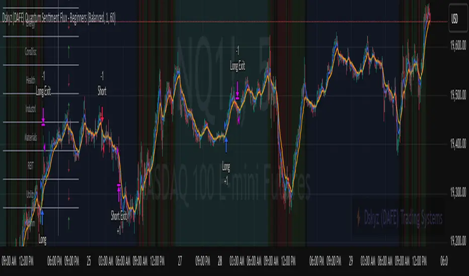
Risultati della ricerca di script per “12月18日油价”

Dskyz (DAFE) Quantum Sentiment Flux - Beginners Dskyz (DAFE) Quantum Sentiment Flux - Beginners: Welcome to the Dskyz (DAFE) Quantum Sentiment Flux - Beginners , a strategy and concept that’s your ultimate wingman for trading futures like MNQ, NQ, MES, and ES. This gem combines lightning-fast momentum signals, market sentiment smarts, and bulletproof risk management into a system so intuitive, even newbies can trade like pros. With clean DAFE visuals, preset modes for every vibe, and a revamped dashboard that’s basically a market GPS, this strategy makes futures trading feel like a high-octane sci-fi mission. Built on the Dskyz (DAFE) legacy of Aurora Divergence, the Quantum Sentiment Flux is designed to empower beginners while giving seasoned traders a lean, sentiment-driven edge. It uses fast/slow EMA crossovers for entries, filters trades with VIX, SPX trends, and sector breadth, and keeps your account safe with adaptive stops and cooldowns. Tuned for more action with faster signals and a slick bottom-left dashboard, this updated version is ready to light up your charts and outsmart institutional traps. Let’s dive into why this strat’s a must-have and break down its brilliance. Why Traders Need This Strategy Futures markets are a wild ride—fast moves, volatility spikes (like the April 28, 2025 NQ 1k-point drop), and institutional games that can wreck unprepared traders. Beginners often get lost in complex systems or burned by impulsive trades. The Quantum Sentiment Flux is the antidote, offering: Dead-Simple Setup: Preset modes (Aggressive, Balanced, Conservative) auto-tune signals, risk, and sizing, so you can trade without a quant degree. Sentiment Superpower: VIX filter, SPX trend, and sector breadth visuals keep you aligned with market health, dodging chop and riding trends. Ironclad Safety: Tighter ATR-based stops, 2:1 take-profits, and preset cooldowns protect your capital, even in chaotic sessions. Next-Level Visuals: Green/red entry triangles, vibrant EMAs, a sector breadth background, and a beefed-up dashboard make signals and context pop. DAFE Swagger: The clean aesthetics, sleek dashboard—ties it to Dskyz’s elite brand, making your charts a work of art. Traders need this because it’s a plug-and-play system that blends beginner-friendly simplicity with pro-level market awareness. Whether you’re just starting or scalping 5min MNQ, this strat’s your key to trading with confidence and style. Strategy Components 1. Core Signal Logic (High-Speed Momentum) The strategy’s engine is a momentum-based system using fast and slow Exponential Moving Averages (EMAs), now tuned for faster, more frequent trades. How It Works: Fast/Slow EMAs: Fast EMA (Aggressive: 5, Balanced: 7, Conservative: 9 bars) and slow EMA (12/14/18 bars) track short-term vs. longer-term momentum. Crossover Signals: Buy: Fast EMA crosses above slow EMA, and trend_dir = 1 (fast EMA > slow EMA + ATR * strength threshold). Sell: Fast EMA crosses below slow EMA, and trend_dir = -1 (fast EMA < slow EMA - ATR * strength threshold). Strength Filter: ma_strength = fast EMA - slow EMA must exceed an ATR-scaled threshold (Aggressive: 0.15, Balanced: 0.18, Conservative: 0.25) for robust signals. Trend Direction: trend_dir confirms momentum, filtering out weak crossovers in choppy markets. Evolution: Faster EMAs (down from 7–10/21–50) catch short-term trends, perfect for active futures markets. Lower strength thresholds (0.15–0.25 vs. 0.3–0.5) make signals more sensitive, boosting trade frequency without sacrificing quality. Preset tuning ensures beginners get optimized settings, while pros can tweak via mode selection. 2. Market Sentiment Filters The strategy leans hard into market sentiment with a VIX filter, SPX trend analysis, and sector breadth visuals, keeping trades aligned with the big picture. VIX Filter: Logic: Blocks long entries if VIX > threshold (default: 20, can_long = vix_close < vix_limit). Shorts are always allowed (can_short = true). Impact: Prevents longs during high-fear markets (e.g., VIX spikes in crashes), while allowing shorts to capitalize on downturns. SPX Trend Filter: Logic: Compares S&P 500 (SPX) close to its SMA (Aggressive: 5, Balanced: 8, Conservative: 12 bars). spx_trend = 1 (UP) if close > SMA, -1 (DOWN) if < SMA, 0 (FLAT) if neutral. Impact: Provides dashboard context, encouraging trades that align with market direction (e.g., longs in UP trend). Sector Breadth (Visual): Logic: Tracks 10 sector ETFs (XLK, XLF, XLE, etc.) vs. their SMAs (same lengths as SPX). Each sector scores +1 (bullish), -1 (bearish), or 0 (neutral), summed as breadth (-10 to +10). Display: Green background if breadth > 4, red if breadth < -4, else neutral. Dashboard shows sector trends (↑/↓/-). Impact: Faster SMA lengths make breadth more responsive, reflecting sector rotations (e.g., tech surging, energy lagging). Why It’s Brilliant: - VIX filter adds pro-level volatility awareness, saving beginners from panic-driven losses. - SPX and sector breadth give a 360° view of market health, boosting signal confidence (e.g., green BG + buy signal = high-probability trade). - Shorter SMAs make sentiment visuals react faster, perfect for 5min charts. 3. Risk Management The risk controls are a fortress, now tighter and more dynamic to support frequent trading while keeping accounts safe. Preset-Based Risk: Aggressive: Fast EMAs (5/12), tight stops (1.1x ATR), 1-bar cooldown. High trade frequency, higher risk. Balanced: EMAs (7/14), 1.2x ATR stops, 1-bar cooldown. Versatile for most traders. Conservative: EMAs (9/18), 1.3x ATR stops, 2-bar cooldown. Safer, fewer trades. Impact: Auto-scales risk to match style, making it foolproof for beginners. Adaptive Stops and Take-Profits: Logic: Stops = entry ± ATR * atr_mult (1.1–1.3x, down from 1.2–2.0x). Take-profits = entry ± ATR * take_mult (2x stop distance, 2:1 reward/risk). Longs: stop below entry, TP above; shorts: vice versa. Impact: Tighter stops increase trade turnover while maintaining solid risk/reward, adapting to volatility. Trade Cooldown: Logic: Preset-driven (Aggressive/Balanced: 1 bar, Conservative: 2 bars vs. old user-input 2). Ensures bar_index - last_trade_bar >= cooldown. Impact: Faster cooldowns (especially Aggressive/Balanced) allow more trades, balanced by VIX and strength filters. Contract Sizing: Logic: User sets contracts (default: 1, max: 10), no preset cap (unlike old 7/5/3 suggestion). Impact: Flexible but risks over-leverage; beginners should stick to low contracts. Built To Be Reliable and Consistent: - Tighter stops and faster cooldowns make it a high-octane system without blowing up accounts. - Preset-driven risk removes guesswork, letting newbies trade confidently. - 2:1 TPs ensure profitable trades outweigh losses, even in volatile sessions like April 27, 2025 ES slippage. 4. Trade Entry and Exit Logic The entry/exit rules are simple yet razor-sharp, now with VIX filtering and faster signals: Entry Conditions: Long Entry: buy_signal (fast EMA crosses above slow EMA, trend_dir = 1), no position (strategy.position_size = 0), cooldown passed (can_trade), and VIX < 20 (can_long). Enters with user-defined contracts. Short Entry: sell_signal (fast EMA crosses below slow EMA, trend_dir = -1), no position, cooldown passed, can_short (always true). Logic: Tracks last_entry_bar for visuals, last_trade_bar for cooldowns. Exit Conditions: Stop-Loss/Take-Profit: ATR-based stops (1.1–1.3x) and TPs (2x stop distance). Longs exit if price hits stop (below) or TP (above); shorts vice versa. No Other Exits: Keeps it straightforward, relying on stops/TPs. 5. DAFE Visuals The visuals are pure DAFE magic, blending clean function with informative metrics utilized by professionals, now enhanced by faster signals and a responsive breadth background: EMA Plots: Display: Fast EMA (blue, 2px), slow EMA (orange, 2px), using faster lengths (5–9/12–18). Purpose: Highlights momentum shifts, with crossovers signaling entries. Sector Breadth Background: Display: Green (90% transparent) if breadth > 4, red (90%) if breadth < -4, else neutral. Purpose: Faster breadth_sma_len (5–12 vs. 10–50) reflects sector shifts in real-time, reinforcing signal strength. - Visuals are intuitive, turning complex signals into clear buy/sell cues. - Faster breadth background reacts to market rotations (e.g., tech vs. energy), giving a pro-level edge. 6. Sector Breadth Dashboard The new bottom-left dashboard is a game-changer, a 3x16 table (black/gray theme) that’s your market command center: Metrics: VIX: Current VIX (red if > 20, gray if not). SPX: Trend as “UP” (green), “DOWN” (red), or “FLAT” (gray). Trade Longs: “OK” (green) if VIX < 20, “BLOCK” (red) if not. Sector Breadth: 10 sectors (Tech, Financial, etc.) with trend arrows (↑ green, ↓ red, - gray). Placeholder Row: Empty for future metrics (e.g., ATR, breadth score). Purpose: Consolidates regime, volatility, market trend, and sector data, making decisions a breeze. - VIX and SPX metrics add context, helping beginners avoid bad trades (e.g., no longs if “BLOCK”). Sector arrows show market health at a glance, like a cheat code for sentiment. Key Features Beginner-Ready: Preset modes and clear visuals make futures trading a breeze. Sentiment-Driven: VIX filter, SPX trend, and sector breadth keep you in sync with the market. High-Frequency: Faster EMAs, tighter stops, and short cooldowns boost trade volume. Safe and Smart: Adaptive stops/TPs and cooldowns protect capital while maximizing wins. Visual Mastery: DAFE’s clean flair, EMAs, dashboard—makes trading fun and clear. Backtestable: Lean code and fixed qty ensure accurate historical testing. How to Use Add to Chart: Load on a 5min MNQ/ES chart in TradingView. Pick Preset: Aggressive (scalping), Balanced (versatile), or Conservative (safe). Balanced is default. Set Contracts: Default 1, max 10. Stick low for safety. Check Dashboard: Bottom-left shows preset, VIX, SPX, and sectors. “OK” + green breadth = strong buy. Backtest: Run in strategy tester to compare modes. Live Trade: Connect to Tradovate or similar. Watch for slippage (e.g., April 27, 2025 ES issues). Replay Test: Try April 28, 2025 NQ drop to see VIX filter and stops in action. Why It’s Brilliant The Dskyz (DAFE) Quantum Sentiment Flux - Beginners is a masterpiece of simplicity and power. It takes pro-level tools—momentum, VIX, sector breadth—and wraps them in a system anyone can run. Faster signals and tighter stops make it a trading machine, while the VIX filter and dashboard keep you ahead of market chaos. The DAFE visuals and bottom-left command center turn your chart into a futuristic cockpit, guiding you through every trade. For beginners, it’s a safe entry to futures; for pros, it’s a scalping beast with sentiment smarts. This strat doesn’t just trade—it transforms how you see the market. Final Notes This is more than a strategy—it’s your launchpad to mastering futures with Dskyz (DAFE) flair. The Quantum Sentiment Flux blends accessibility, speed, and market savvy to help you outsmart the game. Load it, watch those triangles glow, and let’s make the markets your canvas! Official Statement from Pine Script Team (see TradingView help docs and forums): "This warning may appear when you call functions such as ta.sma inside a request.security in a loop. There is no runtime impact. If you need to loop through a dynamic list of tickers, this cannot be avoided in the present version... Values will still be correct. Ignore this warning in such contexts." (This publishing will most likely be taken down do to some miscellaneous rule about properly displaying charting symbols, or whatever. Once I've identified what part of the publishing they want to pick on, I'll adjust and repost.) Use it with discipline. Use it with clarity. Trade smarter. **I will continue to release incredible strategies and indicators until I turn this into a brand or until someone offers me a contract. Created by Dskyz, powered by DAFE Trading Systems. Trade fast, trade bold.

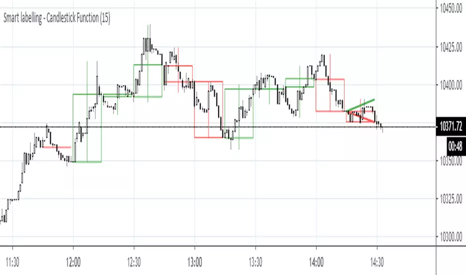
Smart labelling - Candlestick Function Oftentimes a single look at the candlestick configuration happens to be enough to understand what is going on. The chandlestick function is an experiment in smart labelling that produces candles for various time frames, not only for the fixed 1m, 3m , 5m, 15m, etc. ones, and helps in decision-making when eye-balling the chart. This function generates up to 12 last candlesticks , which is generally more than enough. Mind that since this is an experiment, the function does not cover all possible combinations. In some time frames the produced candles overlap. This is a todo item for those who are unterested. For instance, the current version covers the following TFs: Chart - TF in the script 1m - 1-20,24,30,32 3m - 1-10 5m - 1-4,6,9,12,18,36 15m - 1-4,6,12 Tested chart TFs: 1m, 3m ,5m,15m. Tested securities: BTCUSD , EURUSD

Bear Market Probability Model # Bear Market Probability Model: A Multi-Factor Risk Assessment Framework The Bear Market Probability Model represents a comprehensive quantitative framework for assessing systemic market risk through the integration of 13 distinct risk factors across four analytical categories: macroeconomic indicators, technical analysis factors, market sentiment measures, and market breadth metrics. This indicator synthesizes established financial research methodologies to provide real-time probabilistic assessments of impending bear market conditions, offering institutional-grade risk management capabilities to retail and professional traders alike. ## Theoretical Foundation ### Historical Context of Bear Market Prediction Bear market prediction has been a central focus of financial research since the seminal work of Dow (1901) and the subsequent development of technical analysis theory. The challenge of predicting market downturns gained renewed academic attention following the market crashes of 1929, 1987, 2000, and 2008, leading to the development of sophisticated multi-factor models. Fama and French (1989) demonstrated that certain financial variables possess predictive power for stock returns, particularly during market stress periods. Their three-factor model laid the groundwork for multi-dimensional risk assessment, which this indicator extends through the incorporation of real-time market microstructure data. ### Methodological Framework The model employs a weighted composite scoring methodology based on the theoretical framework established by Campbell and Shiller (1998) for market valuation assessment, extended through the incorporation of high-frequency sentiment and technical indicators as proposed by Baker and Wurgler (2006) in their seminal work on investor sentiment. The mathematical foundation follows the general form: Bear Market Probability = Σ(Wi × Ci) / ΣWi × 100 Where: - Wi = Category weight (i = 1,2,3,4) - Ci = Normalized category score - Categories: Macroeconomic, Technical, Sentiment, Breadth ## Component Analysis ### 1. Macroeconomic Risk Factors #### Yield Curve Analysis The inclusion of yield curve inversion as a primary predictor follows extensive research by Estrella and Mishkin (1998), who demonstrated that the term spread between 3-month and 10-year Treasury securities has historically preceded all major recessions since 1969. The model incorporates both the 2Y-10Y and 3M-10Y spreads to capture different aspects of monetary policy expectations. Implementation: - 2Y-10Y Spread: Captures market expectations of monetary policy trajectory - 3M-10Y Spread: Traditional recession predictor with 12-18 month lead time Scientific Basis: Harvey (1988) and subsequent research by Ang, Piazzesi, and Wei (2006) established the theoretical foundation linking yield curve inversions to economic contractions through the expectations hypothesis of the term structure. #### Credit Risk Premium Assessment High-yield credit spreads serve as a real-time gauge of systemic risk, following the methodology established by Gilchrist and Zakrajšek (2012) in their excess bond premium research. The model incorporates the ICE BofA High Yield Master II Option-Adjusted Spread as a proxy for credit market stress. Threshold Calibration: - Normal conditions: < 350 basis points - Elevated risk: 350-500 basis points - Severe stress: > 500 basis points #### Currency and Commodity Stress Indicators The US Dollar Index (DXY) momentum serves as a risk-off indicator, while the Gold-to-Oil ratio captures commodity market stress dynamics. This approach follows the methodology of Akram (2009) and Beckmann, Berger, and Czudaj (2015) in analyzing commodity-currency relationships during market stress. ### 2. Technical Analysis Factors #### Multi-Timeframe Moving Average Analysis The technical component incorporates the well-established moving average convergence methodology, drawing from the work of Brock, Lakonishok, and LeBaron (1992), who provided empirical evidence for the profitability of technical trading rules. Implementation: - Price relative to 50-day and 200-day simple moving averages - Moving average convergence/divergence analysis - Multi-timeframe MACD assessment (daily and weekly) #### Momentum and Volatility Analysis The model integrates Relative Strength Index (RSI) analysis following Wilder's (1978) original methodology, combined with maximum drawdown analysis based on the work of Magdon-Ismail and Atiya (2004) on optimal drawdown measurement. ### 3. Market Sentiment Factors #### Volatility Index Analysis The VIX component follows the established research of Whaley (2009) and subsequent work by Bekaert and Hoerova (2014) on VIX as a predictor of market stress. The model incorporates both absolute VIX levels and relative VIX spikes compared to the 20-day moving average. Calibration: - Low volatility: VIX < 20 - Elevated concern: VIX 20-25 - High fear: VIX > 25 - Panic conditions: VIX > 30 #### Put-Call Ratio Analysis Options flow analysis through put-call ratios provides insight into sophisticated investor positioning, following the methodology established by Pan and Poteshman (2006) in their analysis of informed trading in options markets. ### 4. Market Breadth Factors #### Advance-Decline Analysis Market breadth assessment follows the classic work of Fosback (1976) and subsequent research by Brown and Cliff (2004) on market breadth as a predictor of future returns. Components: - Daily advance-decline ratio - Advance-decline line momentum - McClellan Oscillator (Ema19 - Ema39 of A-D difference) #### New Highs-New Lows Analysis The new highs-new lows ratio serves as a market leadership indicator, based on the research of Zweig (1986) and validated in academic literature by Zarowin (1990). ## Dynamic Threshold Methodology The model incorporates adaptive thresholds based on rolling volatility and trend analysis, following the methodology established by Pagan and Sossounov (2003) for business cycle dating. This approach allows the model to adjust sensitivity based on prevailing market conditions. Dynamic Threshold Calculation: - Warning Level: Base threshold ± (Volatility × 1.0) - Danger Level: Base threshold ± (Volatility × 1.5) - Bounds: ±10-20 points from base threshold ## Professional Implementation ### Institutional Usage Patterns Professional risk managers typically employ multi-factor bear market models in several contexts: #### 1. Portfolio Risk Management - Tactical Asset Allocation: Reducing equity exposure when probability exceeds 60-70% - Hedging Strategies: Implementing protective puts or VIX calls when warning thresholds are breached - Sector Rotation: Shifting from growth to defensive sectors during elevated risk periods #### 2. Risk Budgeting - Value-at-Risk Adjustment: Incorporating bear market probability into VaR calculations - Stress Testing: Using probability levels to calibrate stress test scenarios - Capital Requirements: Adjusting regulatory capital based on systemic risk assessment #### 3. Client Communication - Risk Reporting: Quantifying market risk for client presentations - Investment Committee Decisions: Providing objective risk metrics for strategic decisions - Performance Attribution: Explaining defensive positioning during market stress ### Implementation Framework Professional traders typically implement such models through: #### Signal Hierarchy: 1. Probability < 30%: Normal risk positioning 2. Probability 30-50%: Increased hedging, reduced leverage 3. Probability 50-70%: Defensive positioning, cash building 4. Probability > 70%: Maximum defensive posture, short exposure consideration #### Risk Management Integration: - Position Sizing: Inverse relationship between probability and position size - Stop-Loss Adjustment: Tighter stops during elevated risk periods - Correlation Monitoring: Increased attention to cross-asset correlations ## Strengths and Advantages ### 1. Comprehensive Coverage The model's primary strength lies in its multi-dimensional approach, avoiding the single-factor bias that has historically plagued market timing models. By incorporating macroeconomic, technical, sentiment, and breadth factors, the model provides robust risk assessment across different market regimes. ### 2. Dynamic Adaptability The adaptive threshold mechanism allows the model to adjust sensitivity based on prevailing volatility conditions, reducing false signals during low-volatility periods and maintaining sensitivity during high-volatility regimes. ### 3. Real-Time Processing Unlike traditional academic models that rely on monthly or quarterly data, this indicator processes daily market data, providing timely risk assessment for active portfolio management. ### 4. Transparency and Interpretability The component-based structure allows users to understand which factors are driving risk assessment, enabling informed decision-making about model signals. ### 5. Historical Validation Each component has been validated in academic literature, providing theoretical foundation for the model's predictive power. ## Limitations and Weaknesses ### 1. Data Dependencies The model's effectiveness depends heavily on the availability and quality of real-time economic data. Federal Reserve Economic Data (FRED) updates may have lags that could impact model responsiveness during rapidly evolving market conditions. ### 2. Regime Change Sensitivity Like most quantitative models, the indicator may struggle during unprecedented market conditions or structural regime changes where historical relationships break down (Taleb, 2007). ### 3. False Signal Risk Multi-factor models inherently face the challenge of balancing sensitivity with specificity. The model may generate false positive signals during normal market volatility periods. ### 4. Currency and Geographic Bias The model focuses primarily on US market indicators, potentially limiting its effectiveness for global portfolio management or non-USD denominated assets. ### 5. Correlation Breakdown During extreme market stress, correlations between risk factors may increase dramatically, reducing the model's diversification benefits (Forbes and Rigobon, 2002). ## References Akram, Q. F. (2009). Commodity prices, interest rates and the dollar. Energy Economics, 31(6), 838-851. Ang, A., Piazzesi, M., & Wei, M. (2006). What does the yield curve tell us about GDP growth? Journal of Econometrics, 131(1-2), 359-403. Baker, M., & Wurgler, J. (2006). Investor sentiment and the cross‐section of stock returns. The Journal of Finance, 61(4), 1645-1680. Baker, S. R., Bloom, N., & Davis, S. J. (2016). Measuring economic policy uncertainty. The Quarterly Journal of Economics, 131(4), 1593-1636. Barber, B. M., & Odean, T. (2001). Boys will be boys: Gender, overconfidence, and common stock investment. The Quarterly Journal of Economics, 116(1), 261-292. Beckmann, J., Berger, T., & Czudaj, R. (2015). Does gold act as a hedge or a safe haven for stocks? A smooth transition approach. Economic Modelling, 48, 16-24. Bekaert, G., & Hoerova, M. (2014). The VIX, the variance premium and stock market volatility. Journal of Econometrics, 183(2), 181-192. Brock, W., Lakonishok, J., & LeBaron, B. (1992). Simple technical trading rules and the stochastic properties of stock returns. The Journal of Finance, 47(5), 1731-1764. Brown, G. W., & Cliff, M. T. (2004). Investor sentiment and the near-term stock market. Journal of Empirical Finance, 11(1), 1-27. Campbell, J. Y., & Shiller, R. J. (1998). Valuation ratios and the long-run stock market outlook. The Journal of Portfolio Management, 24(2), 11-26. Dow, C. H. (1901). Scientific stock speculation. The Magazine of Wall Street. Estrella, A., & Mishkin, F. S. (1998). Predicting US recessions: Financial variables as leading indicators. Review of Economics and Statistics, 80(1), 45-61. Fama, E. F., & French, K. R. (1989). Business conditions and expected returns on stocks and bonds. Journal of Financial Economics, 25(1), 23-49. Forbes, K. J., & Rigobon, R. (2002). No contagion, only interdependence: measuring stock market comovements. The Journal of Finance, 57(5), 2223-2261. Fosback, N. G. (1976). Stock market logic: A sophisticated approach to profits on Wall Street. The Institute for Econometric Research. Gilchrist, S., & Zakrajšek, E. (2012). Credit spreads and business cycle fluctuations. American Economic Review, 102(4), 1692-1720. Harvey, C. R. (1988). The real term structure and consumption growth. Journal of Financial Economics, 22(2), 305-333. Kahneman, D., & Tversky, A. (1979). Prospect theory: An analysis of decision under risk. Econometrica, 47(2), 263-291. Magdon-Ismail, M., & Atiya, A. F. (2004). Maximum drawdown. Risk, 17(10), 99-102. Nickerson, R. S. (1998). Confirmation bias: A ubiquitous phenomenon in many guises. Review of General Psychology, 2(2), 175-220. Pagan, A. R., & Sossounov, K. A. (2003). A simple framework for analysing bull and bear markets. Journal of Applied Econometrics, 18(1), 23-46. Pan, J., & Poteshman, A. M. (2006). The information in option volume for future stock prices. The Review of Financial Studies, 19(3), 871-908. Taleb, N. N. (2007). The black swan: The impact of the highly improbable. Random House. Whaley, R. E. (2009). Understanding the VIX. The Journal of Portfolio Management, 35(3), 98-105. Wilder, J. W. (1978). New concepts in technical trading systems. Trend Research. Zarowin, P. (1990). Size, seasonality, and stock market overreaction. Journal of Financial and Quantitative Analysis, 25(1), 113-125. Zweig, M. E. (1986). Winning on Wall Street. Warner Books.

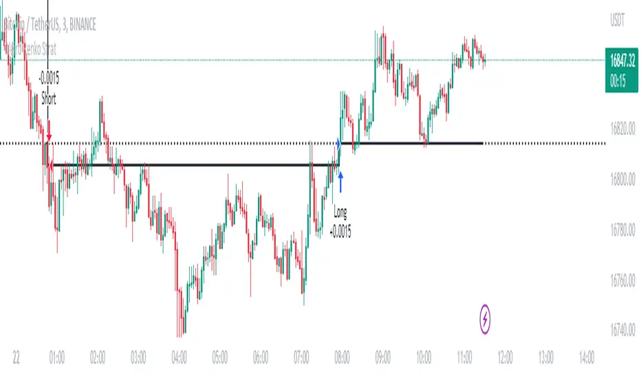
Weird Renko Strat This strategy uses Renko, it generates a signal when there is a reversal in Renko. When using historical data, it provides a good entry and an okay exit. However, in a real-time environment, this strategy is subject to repaint and may produce a false signal. As a result, the backtesting result should not be used as a metric to predict future results. It is highly recommended to forward-test the strategy before using it in real trading. I forward test it from 12/18/2022 to 12/21/2022 in paper trading, using the alert feature in Tradingview. I made 60 trades trading the BTCUSDT BINANCE 3 min with 26 as the param and under the condition that I use 20x margin, compounding my yield, and having 0 trading fee, a steady loss is generated: from $10 to $3.02. This is quite interesting. As if I flip the signal from "Long" to "Short" and another way too, it will be a steady profit from $10 to $21.85. Hence, if I'm trying to anti-trade the real-time alert signal, the current "4 Days Result" will be good. Nevertheless, I still have to forward-test it for longer to see if it will fail eventually. Dive into the setting of the strategy - Margin is the leverage you use. 1 means 1x, 10 means 10x. It affects the backtest yield when you backtest - Compound Yield button is for compound calculation, disable it to go back to normal backtesting - Anti Strategy button is to do the opposite direction trade, when the original strat told you to "Long", you "Short" instead. Enable it to use the feature - Param is the block size for the Renko chart - Drawdown is just a visual tool for you in case you want to place a stop loss (represent by the semitransparent red area in the chart) - From date Thru Date is to specify the backtest range of the strategy, This feature is turned off by default. It is controlled by the Max Backtest Timeframe which will be explain below - Max Backtest Timeframe control the From date Thru Date function, disable it to enable the From Date Thru Date function Param is the most important input in this strategy as it directly affects performance. It is highly recommended to backtest nearly all the possible parameters before deploying it in real trading. Some factors should be considered: - Price of the asset (like an asset of 1 USD vs an asset of 10000 USD required different param) - Timeframe (1-minute param is different than 1-month param) I believe this is caused by the volatility of the selected timeframe since different timeframe has different volatility. Param should be fine-tuned before usage. Here is the param I'm using: BTCUSDT BINANCE 3min: 26 BTCUSDT BINANCE 5min: 28 BTCUSDT BINANCE 1day: 15 Background of the strategy: - The strategy starts with $10 at the start of backtesting (customizable in setting) - The trading fee is set to 0.00% which is not common for most of the popular exchanges (customizable in setting) - The contract size is not a fixed amount, but it uses your balance to buy it at the open price. If you are using the compound mode, your balance will be your current total balance. If you are using the non-compound mode, it will just use the $10 you start with unless you change the amount you start with. If you are using a margin higher than 1, it will calculate the corresponding contract size properly based on your margin. (Only these options are allowed, you are not able to change them without changing the code)

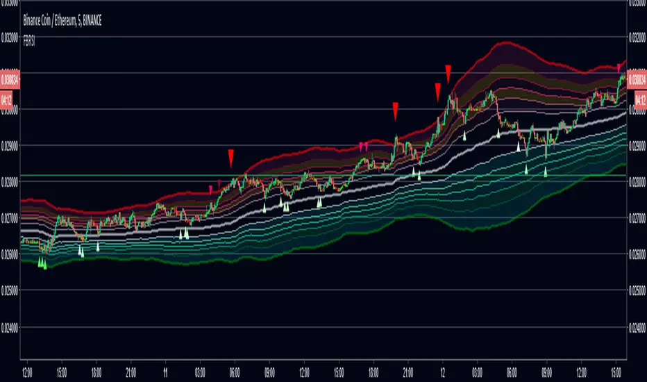
FIB Band Signals with RSI Filter Original Author: Rashad Added by Rashad 6-26-16 These Bollinger bands feature Fibonacci retracements to very clearly show areas of support and resistance . The basis is calculate off of the Volume Weighted Moving Average . The Bands are 3 standard deviations away from the mean. 99.73% of observations should be in this range. Updated by Dysrupt 7-12-18 -Buy signals added on lower bands, mean and upper 3 bands -Sell signals added to upper 3 bands -RSI filter applied to signals -Alerts not yet added -Long Biased NOTE: This is NOT a set and forget signal indicator. It is extremely versatile for all environments by adjusting the RSI filter and checking the band signals needed for the current trend and trading style.

666 & BK Method This method uses common numbers which rule the word, 666, so ma 6,12,18,66,180 and the boss method whose ma 7, 14, 21, 77, 231.

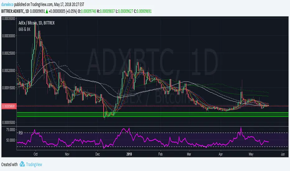
666 & BK This method uses common numbers which rule the word, 666, so ma 6,12,18,66,180 and the boss method whose ma 7, 14, 21, 77, 231.