Prodotti
Comunità
Mercati
Broker
Altro

Comunità
Indicatori e strategie
Risultati della ricerca

Cerca negli script per "20蒙古币兑换人民币"

T-Virus Sentiment [hapharmonic]🧬 T-Virus Sentiment: Visualize the Market's DNA Remember the iconic T-Virus vial from the first Resident Evil? That powerful, swirling helix of potential has always fascinated me. It sparked an idea: what if we could visualize the market's underlying health in a similar way? What if we could capture the "genetic code" of market sentiment and contain it within a dynamic, 3D indicator? This project is the result of that idea, brought to life with Pine Script. The indicator's main goal is to measure the strength and direction of market sentiment by analyzing the "genetic code" of price action through a variety of trusted indicators. The result is displayed as a liquid level within a DNA helix, a bubble density representing buying pressure, and a T-Virus mascot that reflects the overall mood. 🧐 Core Concept: How It Works The primary output of the indicator is the "Active %" gauge you see on the right side of the vial. This percentage represents the overall sentiment score, calculated as an average from 7 different technical analysis tools. Each tool is analyzed on every bar and assigned a score from 1 (strong bearish pressure) to 5 (strong bullish potential). In this indicator, we re-imagine market dynamics through the lens of a viral outbreak. A strong bear market is like a virus taking hold, pulling all technical signals down into a state of weakness. Conversely, a powerful bull market is like an antiviral serum ; positive signals rise and spread toward the top of the vial, indicating that the system is being injected with strength. This is not just another line on a chart. It's a comprehensive sentiment dashboard designed to give an immediate, at-a-glance understanding of the confluence between 7 classic technical indicators. The incredible 3D model of the vial itself was inspired by a design concept found here . ⚛️ The 4 Core Elements of T-Virus Sentiment These four elements work in harmony to give a complete, multi-faceted picture of market sentiment. Each component tells a different part of the story. The Virus Mascot: An instant emotional cue. This character provides the quickest possible read on the overall market mood, combining sentiment with volume pressure. The Antiviral Serum Level: The main quantitative output. This is the liquid level in the DNA helix and the percentage gauge on the right, representing the average sentiment score from all 7 indicators. Buy Pressure & Bubble Density: This visualizes volume flow. The density of bubbles represents the intensity of accumulation (buying) versus distribution (selling). It's the "power" behind the move. The Signal Distribution: This shows the confluence (or dispersion) of sentiment. Are all signals bullish and clustered at the top, or are they scattered, indicating a conflicted market? The position of the indicator labels is crucial, as each is assigned to one of five distinct zones: Base Bottom: The market is at its weakest. Signals here suggest strong bearish control and distribution. Lower Zone: The market is still bearish, but signals may be showing early signs of accumulation or bottoming. Neutral Core (Center): A state of balance or sideways consolidation. The market is waiting for a new direction. Upper Zone: Bullish momentum is becoming clear. Signals are strengthening and showing bullish control. Top Cap: The market is "heating up" with strong bullish sentiment, potentially nearing overbought conditions. 🐂🐻 The Virus Mascot: The At-a-Glance Indicator This character acts as a shortcut to confirm market health. It combines the sentiment score with volume, preventing false confidence in a low-volume rally. Its state is determined by a dual-check: the overall "Antiviral Serum Level" and the "Buy Pressure" must both be above 50%. Green & Smiling: The 'all clear' signal. This means that not only is the overall technical sentiment bullish, but it's also being supported by real buying pressure. This is a sign of a healthy bull market. Red & Angry: A warning sign. This appears if either the sentiment is weak, or a bullish sentiment is not being confirmed by buying volume. The latter could indicate a potential "bull trap" or an exhaustive move. This mascot can be disabled from the settings page under "Virus Mascot Styling" if a cleaner look is preferred. 🫧 Bubble Density: Gauging Buy vs. Sell Pressure The bubbles visualize the battle between buyers and sellers. There are two modes to control how this is calculated: Mode 1: Visible Range (The 'Big Picture' View) This default mode is best for getting a broad, contextual understanding of the current session. It dynamically analyzes the volume of every single candlestick currently visible on the screen to calculate the buy/sell pressure ratio. It answers the question: "Over the entire period I'm looking at, who is in control?" As you zoom in or out, the calculation adapts. Mode 2: Custom Lookback (The 'Precision' View) This mode is for traders who need to analyze short-term pressure. You can define a fixed number of recent bars to analyze, which is perfect for scalping or understanding the volume dynamics leading into a key level. It answers the question: "What is happening right now ?" In the example above, a lookback of 2 focuses only on the most recent action, clearly showing intense, immediate selling pressure (few bubbles) and a corresponding drop in the sentiment score to 29%. ℹ️ Interactive Tooltips: Dive Deeper We believe in transparency, not 'black box' indicators. This feature transforms the indicator from a visual aid into an active learning tool. Simply hover the mouse over any indicator label (like EMA, OBV, etc.) to get a detailed tooltip. It will explain the specific data points and thresholds that signal met to be placed in its current zone. This helps build trust in the signals and allows users to fine-tune the indicator settings to better match their own trading style. 🎯 The Scoring Logic Breakdown The "Antiviral Serum Level" gauge is the average score from 7 technical analysis tools. Each is graded on a 5-point scale (1=Strong Bearish to 5=Strong Bullish). Here’s a detailed, transparent look at how each "gene" is evaluated: Relative Strength Index (RSI) Measures momentum and overbought/oversold conditions. Group 1 (Strong Bearish): RSI > 80 (Extreme Overbought) Group 2 (Bearish): 70 < RSI ≤ 80 (Overbought) Group 3 (Neutral): 30 ≤ RSI ≤ 70 Group 4 (Bullish): 20 ≤ RSI < 30 (Oversold) Group 5 (Strong Bullish): RSI < 20 (Extreme Oversold) Exponential Moving Averages (EMA) Evaluates the trend's strength and structure based on the alignment of multiple EMAs (9, 21, 50, 100, 200, 250). Group 1 (Strong Bearish): A perfect bearish sequence (9 < 21 < 50 < ...) Group 2 (Bearish Transition): Early signs of a potential reversal (e.g., 9 > 21 but still below 50) Group 3 (Neutral / Mixed): MAs are intertwined or showing a partial bullish sequence. Group 4 (Bullish): A strong bullish sequence is forming (e.g., 9 > 21 > 50 > 100) Group 5 (Strong Bullish): A perfect bullish sequence (9 > 21 > 50 > 100 > 200 > 250) Moving Average Convergence Divergence (MACD) Analyzes the relationship between two moving averages to gauge momentum. Group 1 (Strong Bearish): MACD & Histogram are negative and momentum is falling. Group 2 (Weakening Bearish): MACD is negative but the histogram is rising or positive. Group 3 (Neutral / Crossover): A crossover event is occurring near the zero line. Group 4 (Bullish): MACD & Histogram are positive. Group 5 (Strong Bullish): MACD & Histogram are positive, rising strongly, and accelerating. Average Directional Index (ADX) Measures trend strength, not direction. The score is based on both ADX value and the dominance of DI+ vs DI-. Group 1 (Bearish / No Trend): ADX < 20 and DI- is dominant. Group 2 (Developing Bearish Trend): 20 ≤ ADX < 25 and DI- is dominant. Group 3 (Neutral / Indecision): Trend is weak or DI+ and DI- are nearly equal. Group 4 (Developing Bullish Trend): 25 ≤ ADX ≤ 40 and DI+ is dominant. Group 5 (Strong Bullish Trend): ADX > 40 and DI+ is dominant. Ichimoku Cloud (IKH) A comprehensive indicator that defines support/resistance, momentum, and trend direction. Group 1 (Strong Bearish): Price is below the Kumo, Tenkan < Kijun, and Chikou is below price. Group 2 (Bearish): Price is inside or below the Kumo, with mixed secondary signals. Group 3 (Neutral / Ranging): Price is inside the Kumo, often with a Tenkan/Kijun cross. Group 4 (Bullish): Price is above the Kumo with strong primary signals. Group 5 (Strong Bullish): All signals are aligned bullishly: price above Kumo, bullish Tenkan/Kijun cross, bullish future Kumo, and Chikou above price. Bollinger Bands (BB) Measures volatility and relative price levels. Group 1 (Strong Bearish): Price is below the lower band. Group 2 (Bearish Territory): Price is between the lower band and the basis line. Group 3 (Neutral): Price is hovering around the basis line. Group 4 (Bullish Territory): Price is between the basis line and the upper band. Group 5 (Strong Bullish): Price is above the upper band. On-Balance Volume (OBV) Uses volume flow to predict price changes. The score is based on OBV's trend and its position relative to its moving average. Group 1 (Strong Bearish): OBV is below its MA and falling. Group 2 (Weakening Bearish): OBV is below its MA but showing signs of rising. Group 3 (Neutral): OBV is very close to its MA. Group 4 (Bullish): OBV is above its MA and rising. Group 5 (Strong Bullish): OBV is above its MA, rising strongly, and showing signs of a volume spike. 🧭 How to Use the T-Virus Sentiment Indicator IMPORTANT: This indicator is a sentiment dashboard , not a direct buy/sell signal generator. Its strength lies in showing confluence and providing a quick, holistic view of the market's technical health. Confirmation Tool: Use the "Active %" gauge to confirm a trade setup from your primary strategy. For example, if you see a bullish chart pattern, a high and rising sentiment score can add confidence to your trade. Momentum & Trend Gauge: A consistently high score (e.g., > 75%) suggests strong, established bullish momentum. A consistently low score (< 25%) suggests strong bearish control. A score hovering around 50% often indicates a ranging or indecisive market. Divergence & Warning System: Pay attention to divergences. If the price is making new highs but the sentiment score is failing to follow or is actively decreasing, it could be an early warning sign that the underlying momentum is weakening. ⚙️ Settings & Customization The indicator is highly customizable to fit any trading style. Position & Anchor: Control where the vial appears on the chart. Styling (Vial, Helix, etc.): Nearly every visual element can be color-customized. Signals: This is where the real power is. All underlying indicator parameters (RSI length, MACD settings, etc.) can be fine-tuned to match a personal strategy. The text labels can also be disabled if the chart feels cluttered. Enjoy visualizing the market's DNA with the T-Virus Sentiment indicator

Indicatore Pine Script®

Aggiornato

Reversal Radars — Berk v2.0 (Bottom & Top)1) Combined script (Dip+Tepe) Title: Reversal Radars — Berk v2.0 (Bottom & Top) Description (EN): What it does Two high-probability reversal detectors in one indicator: a Bottom Reversal Radar (long bias) and a Top Reversal Radar (short/hedge bias). Each radar aggregates multiple conditions into a single score and triggers when Score ≥ Threshold. How it works RSI regime shift: Bottom = recovery after oversold (touched 30, crosses up 35). Top = roll-over from overbought (touched 70, crosses down 65). MACD cross: Bull (up) for bottoms, Bear (down) for tops. EMA8 filter: Close above (bottom) / below (top) EMA(8). Structure break (BOS): Close above recent swing high / below recent swing low (lookbackBars, using precomputed highest/lowest to avoid inconsistencies). EMA200 proximity: Price within a configurable band (default −5% … +2%). Volume expansion: Volume ≥ SMA(20) × multiplier (default 1.5×). Divergence: Pivot-confirmed (3/3) bullish (bottom) or bearish (top) RSI divergence. Scoring: RSI shift +2, divergence +2, MACD +1, EMA8 +1, BOS +1, Volume +1, EMA200 band +1. Signals & Alerts Bottom: label “DÖNÜŞ↑” and alert “Dipten Dönüş — Ana Sinyal” when scoreLong ≥ thrLong. Top: label “DÖNÜŞ↓” and alert “Tepeden Dönüş — Ana Sinyal” when scoreShort ≥ thrShort. Use Once per bar close for stable alerts. Inputs lenRSI, rsiOS=30, rsiRecover=35, rsiOB=70, rsiFall=65, volLen=20, volMult=1.5, lookbackBars=5, ema200 band (−5…+2%), thrLong/thrShort, toggles for Bottom/Top. Timeframes & tips Best on Daily/4H. Tighten thresholds (e.g., 4) and raise volume multiplier (1.8–2.0×) on lower TFs or thin liquidity. No-repaint note Evaluated on bar close; pivot divergences confirm with a natural ~3-bar delay. Disclaimer Educational use only. Not financial advice. Tags: reversal, divergence, rsi, macd, ema, volume, trend, screener, stocks, crypto, bist 2) Bottom-only (Dip) Title: Bottom Reversal Radar — Berk v1.4 Description (EN): Purpose Scores bottoming conditions and triggers when Score ≥ Threshold (default 3). Components RSI recovery after oversold (30→35), MACD bull cross, close above EMA8, BOS above recent swing high, near-EMA200 band (−5…+2%), volume ≥ SMA(20)×1.5, and pivot-confirmed (3/3) bullish RSI divergence. Weights: RSI +2, Divergence +2, others +1. Usage Add to chart, set alert “Dipten Dönüş — Ana Sinyal”, Once per bar close. Works on any timeframe (need ≥200 bars for EMA200). Daily/4H recommended. No-repaint Bar-close evaluation; divergence confirms with ~3 bars. Tags: bottom, reversal, rsi, macd, ema, volume, divergence 3) Top-only (Tepe) Title: Top Reversal Radar — Berk v1.0 Description (EN): Purpose Detects topping risk and triggers when Score ≥ Threshold (default 3) for exits/hedges. Components RSI roll-over from overbought (70→65), MACD bear cross, close below EMA8, BOS below recent swing low, near-EMA200 band, volume ≥ SMA(20)×1.5, and pivot-confirmed (3/3) bearish RSI divergence. Weights: RSI +2, Divergence +2, others +1. Usage Add to chart, set alert “Tepeden Dönüş — Ana Sinyal”, Once per bar close. Daily/4H preferred; tighten thresholds on lower TFs. No-repaint Bar-close evaluation; divergence confirms with ~3 bars. Tags: top, reversal, rsi, macd, ema, volume, divergence

Indicatore Pine Script®

Extended CANSLIM Indicator ❖ Extended CANSLIM Indicator. The Extended CANSLIM indicator is an indicator that concentrates all the tools usually used by CANSLIM traders. It shows a table where all the stock fundamental information is shown at once first for the last quarter and then up to 5 years back. The fundamental data is checked against well known CANSLIM validation criteria and is shown over 4 state levels. 1. Good = Value is CANSLIM Compliant. 2. Acceptable = Value is not CANSLIM compliant but still good. value is shown with a lighter background color. 3. Warning = Value deserves special attention. Value is shown over orange background color. 3. Stop = Value is non CANSLIM compliant or indicates a stop trading condition. Value is shown over red background color. The indicator has also a set of technical tools calculated on price or index and shown directly on the chart. ❖ Fundamental data shown in the table. The table is arranged in 4 sets of data: 1. Table Header, showing Indicator and Company data. 2. CANSLIM. 3. 3Rs: RS Rating, Revenue and ROE. 4. Extra Data: Piotroski score, ATR, Trend Days, D to E, Avg Vol and Vol today. Sets 3 and 4 can be hidden from the table. ❖ Indicator and Compay Data. The table header shows, Indicator name and version. It then displays Company Name, sector and industry, human size and its capitalization. ❖ CANSLIM Data. Displays either genuine CANSLIM data from TradinView or custom data as best effort when that data cannot be obtained in TV. C = EPS diluted growth, Quarterly YoY. >= 25% = Good, >= 0% = Acceptable, < 0% = Stop A = EPS diluted growth, Annual YoY. >= 25% = Good, >= 0% = Acceptable, < 0% = Stop N = New High as best effort (Cust). Always Good S = Float shares as best effort. Always Good L = One year performance relative to S&P 500 (Cust), Positive : 0% .. 50% = Neutral, 50%+ = Leader, 80%+ = Leader+, 100%+ = Leader++ Negative : 0% .. -10% = Laggard, -10% .. -30% = Laggard+, -30%+ = Laggard++ >= 50% = Good, >= 0% = Acceptable, >= -10% Warning, < -10% = Stop I = Accumulation/Distribution days over last 25 days as a clue for institutional support (Cust). A delta is calculated by subtracting Distribution to Accumulation days. > 0 = Good, = 0 = Acceptable, < 0 = Warning, < -5 = Stop M = Market direction and exposure measured on S&500 closing between averages (Cust). Varies from 0% Full Bear to 100% Full Bull >= 80% = Good, >= 60% = Acceptable, >= 40% = Warning, < 40% = Stop ❖ Extra non CANSLIM Data. RS = RS Rating. >= 90 = Good, >= 80 = Accept, >= 50 = Warning, < 50 = Stop Rev. = Revenue Growth Quarterly YoY. >= 0% = Good, <0% = Stop ROE = Return on Equity, Quarterly YoY. >= 17% = Good, >= 0% = Acceptable, < 0% = Stop Piotr. = Piotroski Score, www.investopedia.com (TV) >= 7 = Good, >= 4 = Acceptable, < 4 = Stop ATR = Average True Range over the last 20 days (Cust). 0% - 2% = Acceptable, 2% - 4% = Ideal, 4% - 6% = Warning, 5%+ = Stop. Trend Days = Days since EMA150 is over EMA200 (Cust). Always Good D. to E. = Days left before Earnings. Maybe not a good idea buying just before earnings (Cust). >= 28 = Good, >= 21 = Acceptable, >= 14 = Warning, < 14 = Stop Avg Vol. = 50d Average Volume (Cust). >= 100K = Good, < 100K = Acceptable Vol. Today = Today's percentage volume compared to 50d average (Cust). Always Good. ❖ Historical Data. Optionally selectable historical data can be displayed for C, A, Revenue and ROE up to 20 quarters if available. Quarterly numbers can also be displayed for A, C and Revenue. Information can be shown in Chronological or Reverse Chronological order (default). Increasing growth quarters are shown in white, while diminuing ones are shown in Yellow. Transition from Losing to Profitable quarters are shown with an exclamation mark ‘!’ Finally, losing quarters are shown between parenthesis. ❖ MAs on chart. Displays 200, 100, 50 and 20 days MAs on chart. The MAs are also automatically scaled in the 1W time frame. ❖ New 52 Week High on chart. A sun is shown on the chart the first time that a new 52 week high is reached. The N cell shows a filled sun when a 52 week high is no older than a month, an lighter sun when it’s no older than a quarter or a moon otherwise. ❖ Pocket Pivots on chart. Small triangles below the price are signaling pocket pivots. ❖ Bases on chart, formerly Darvas Boxes. Draw bases as defined by Darvas boxes, both top or bottom of bases can be selected to be shown in order to only show resistance or support. ❖ Market exposure/direction indicator. When charting S&P500 (SPX), Nasdaq 100 Index (NDX), Nasdaq composite (IXIC) or Dow Jownes Index (DJIA), the indicator switches to Market Exposure indicator, showing also Accumulation/Distribution days when volume information is available. This indication which varies from 0% to 100% is what is shown under the M letter in the CANSLIM table which is calculated on the S&P500. ❖ Follow Through Days indicator. If you are an adept of the Low-cheat entry, then you will be highly interested by the Follow Through days indicator as measured in the S&P 500 and shown as diamonds on the chart. The follow-through days are calculated on S&P500 but shown in current stock chart so you don’t need to chart the S&P 500 to know that a follow through day occurred. Follow Through days show correctly on Daily time frame and most are also shown on the Weekly time frame as well. They are also classified according to the market zone in which they occur: 0%-5% from peak = Pullback : FT day is not shown. 5%-10% from peak = Minor Correction : Minor FT days is shown. 10%-20% from peak = Correction : Intermediate FT days us shown 20+% from peak = Bear Market : Makor FT days is shown ❖ RS Line and Rating indicator. A RS Line and Rating indicator can be added to the chart. Relative Strength Rating Accuracy. Please note that the RS Rating is not 100% accurate when compared to IBD values. ❖ Earning Line indicator. An Earning Line indicator can be added to the chart. ❖ ATR Bands and ATR Trade calculator. The motivation for this calculator came from my own need to enter trades on volatile stocks where the simple 7% Stop Loss rule doest not work. It simply calculates the number of shares you can buy at any moment based on current stock price and using the lower ATR band as a stop loss. A few words about the ATR Bands. On this indicator the ATR bands are not drawn as a classical channel that follows the price. The lower band is drawn as a support until it’s broken on a closing basis. It can’t be in a down trend. The upper band is drawn as a resistance until it’s broken on a closing basis. It can’t be in an up trend. The idea is that when price starts to fall down from a peak, it should not violate its lower band ATR and that means that we can use that level as a Stop Loss. You must look back for the stock volatility and find out which ATR multiplier works well meaning that the ATR bands are not violated on normal pullbacks. By default, the indicator uses 5x multiplier. ❖ Extra things, visual features and default settings. The first square cell of current quarter displays a check mark ‘V’ if the CANSLIM criteria is OK or acceptable or a cross ‘X’ otherwise. The first square cell of historical C and Rev show respectively the count of last consecutive positive quarters. There are different color themes from “Forest” to “Space” you can chose from to best fit your eyes. You also have different table sizes going from “Micro” to “Huge” for better adjustment to the size of your display. The default settings view show: Pocket Pivots, FT Days, MA50, RS Line and ATR Bands. That's all, Enjoy!

Indicatore Pine Script®

Aggiornato

Markov Chain [3D] | Fractalyst What exactly is a Markov Chain? This indicator uses a Markov Chain model to analyze, quantify, and visualize the transitions between market regimes (Bull, Bear, Neutral) on your chart. It dynamically detects these regimes in real-time, calculates transition probabilities, and displays them as animated 3D spheres and arrows, giving traders intuitive insight into current and future market conditions. How does a Markov Chain work, and how should I read this spheres-and-arrows diagram? Think of three weather modes: Sunny, Rainy, Cloudy. Each sphere is one mode. The loop on a sphere means “stay the same next step” (e.g., Sunny again tomorrow). The arrows leaving a sphere show where things usually go next if they change (e.g., Sunny moving to Cloudy). Some paths matter more than others. A more prominent loop means the current mode tends to persist. A more prominent outgoing arrow means a change to that destination is the usual next step. Direction isn’t symmetric: moving Sunny→Cloudy can behave differently than Cloudy→Sunny. Now relabel the spheres to markets: Bull, Bear, Neutral. Spheres: market regimes (uptrend, downtrend, range). Self‑loop: tendency for the current regime to continue on the next bar. Arrows: the most common next regime if a switch happens. How to read: Start at the sphere that matches current bar state. If the loop stands out, expect continuation. If one outgoing path stands out, that switch is the typical next step. Opposite directions can differ (Bear→Neutral doesn’t have to match Neutral→Bear). What states and transitions are shown? The three market states visualized are: Bullish (Bull): Upward or strong-market regime. Bearish (Bear): Downward or weak-market regime. Neutral: Sideways or range-bound regime. Bidirectional animated arrows and probability labels show how likely the market is to move from one regime to another (e.g., Bull → Bear or Neutral → Bull). How does the regime detection system work? You can use either built-in price returns (based on adaptive Z-score normalization) or supply three custom indicators (such as volume, oscillators, etc.). Values are statistically normalized (Z-scored) over a configurable lookback period. The normalized outputs are classified into Bull, Bear, or Neutral zones. If using three indicators, their regime signals are averaged and smoothed for robustness. How are transition probabilities calculated? On every confirmed bar, the algorithm tracks the sequence of detected market states, then builds a rolling window of transitions. The code maintains a transition count matrix for all regime pairs (e.g., Bull → Bear). Transition probabilities are extracted for each possible state change using Laplace smoothing for numerical stability, and frequently updated in real-time. What is unique about the visualization? 3D animated spheres represent each regime and change visually when active. Animated, bidirectional arrows reveal transition probabilities and allow you to see both dominant and less likely regime flows. Particles (moving dots) animate along the arrows, enhancing the perception of regime flow direction and speed. All elements dynamically update with each new price bar, providing a live market map in an intuitive, engaging format. Can I use custom indicators for regime classification? Yes! Enable the "Custom Indicators" switch and select any three chart series as inputs. These will be normalized and combined (each with equal weight), broadening the regime classification beyond just price-based movement. What does the “Lookback Period” control? Lookback Period (default: 100) sets how much historical data builds the probability matrix. Shorter periods adapt faster to regime changes but may be noisier. Longer periods are more stable but slower to adapt. How is this different from a Hidden Markov Model (HMM)? It sets the window for both regime detection and probability calculations. Lower values make the system more reactive, but potentially noisier. Higher values smooth estimates and make the system more robust. How is this Markov Chain different from a Hidden Markov Model (HMM)? Markov Chain (as here): All market regimes (Bull, Bear, Neutral) are directly observable on the chart. The transition matrix is built from actual detected regimes, keeping the model simple and interpretable. Hidden Markov Model: The actual regimes are unobservable ("hidden") and must be inferred from market output or indicator "emissions" using statistical learning algorithms. HMMs are more complex, can capture more subtle structure, but are harder to visualize and require additional machine learning steps for training. A standard Markov Chain models transitions between observable states using a simple transition matrix, while a Hidden Markov Model assumes the true states are hidden (latent) and must be inferred from observable “emissions” like price or volume data. In practical terms, a Markov Chain is transparent and easier to implement and interpret; an HMM is more expressive but requires statistical inference to estimate hidden states from data. Markov Chain: states are observable; you directly count or estimate transition probabilities between visible states. This makes it simpler, faster, and easier to validate and tune. HMM: states are hidden; you only observe emissions generated by those latent states. Learning involves machine learning/statistical algorithms (commonly Baum–Welch/EM for training and Viterbi for decoding) to infer both the transition dynamics and the most likely hidden state sequence from data. How does the indicator avoid “repainting” or look-ahead bias? All regime changes and matrix updates happen only on confirmed (closed) bars, so no future data is leaked, ensuring reliable real-time operation. Are there practical tuning tips? Tune the Lookback Period for your asset/timeframe: shorter for fast markets, longer for stability. Use custom indicators if your asset has unique regime drivers. Watch for rapid changes in transition probabilities as early warning of a possible regime shift. Who is this indicator for? Quants and quantitative researchers exploring probabilistic market modeling, especially those interested in regime-switching dynamics and Markov models. Programmers and system developers who need a probabilistic regime filter for systematic and algorithmic backtesting: The Markov Chain indicator is ideally suited for programmatic integration via its bias output (1 = Bull, 0 = Neutral, -1 = Bear). Although the visualization is engaging, the core output is designed for automated, rules-based workflows—not for discretionary/manual trading decisions. Developers can connect the indicator’s output directly to their Pine Script logic (using input.source()), allowing rapid and robust backtesting of regime-based strategies. It acts as a plug-and-play regime filter: simply plug the bias output into your entry/exit logic, and you have a scientifically robust, probabilistically-derived signal for filtering, timing, position sizing, or risk regimes. The MC's output is intentionally "trinary" (1/0/-1), focusing on clear regime states for unambiguous decision-making in code. If you require nuanced, multi-probability or soft-label state vectors, consider expanding the indicator or stacking it with a probability-weighted logic layer in your scripting. Because it avoids subjectivity, this approach is optimal for systematic quants, algo developers building backtested, repeatable strategies based on probabilistic regime analysis. What's the mathematical foundation behind this? The mathematical foundation behind this Markov Chain indicator—and probabilistic regime detection in finance—draws from two principal models: the (standard) Markov Chain and the Hidden Markov Model (HMM). How to use this indicator programmatically? The Markov Chain indicator automatically exports a bias value (+1 for Bullish, -1 for Bearish, 0 for Neutral) as a plot visible in the Data Window. This allows you to integrate its regime signal into your own scripts and strategies for backtesting, automation, or live trading. Step-by-Step Integration with Pine Script (input.source) Add the Markov Chain indicator to your chart. This must be done first, since your custom script will "pull" the bias signal from the indicator's plot. In your strategy, create an input using input.source() Example: //@version=5 strategy("MC Bias Strategy Example") mcBias = input.source(close, "MC Bias Source") After saving, go to your script’s settings. For the “MC Bias Source” input, select the plot/output of the Markov Chain indicator (typically its bias plot). Use the bias in your trading logic Example (long only on Bull, flat otherwise): if mcBias == 1 strategy.entry("Long", strategy.long) else strategy.close("Long") For more advanced workflows, combine mcBias with additional filters or trailing stops. How does this work behind-the-scenes? TradingView’s input.source() lets you use any plot from another indicator as a real-time, “live” data feed in your own script (source). The selected bias signal is available to your Pine code as a variable, enabling logical decisions based on regime (trend-following, mean-reversion, etc.). This enables powerful strategy modularity : decouple regime detection from entry/exit logic, allowing fast experimentation without rewriting core signal code. Integrating 45+ Indicators with Your Markov Chain — How & Why The Enhanced Custom Indicators Export script exports a massive suite of over 45 technical indicators—ranging from classic momentum (RSI, MACD, Stochastic, etc.) to trend, volume, volatility, and oscillator tools—all pre-calculated, centered/scaled, and available as plots. // Enhanced Custom Indicators Export - 45 Technical Indicators // Comprehensive technical analysis suite for advanced market regime detection //@version=6 indicator('Enhanced Custom Indicators Export | Fractalyst', shorttitle='Enhanced CI Export', overlay=false, scale=scale.right, max_labels_count=500, max_lines_count=500) // |----- Input Parameters -----| // momentum_group = "Momentum Indicators" trend_group = "Trend Indicators" volume_group = "Volume Indicators" volatility_group = "Volatility Indicators" oscillator_group = "Oscillator Indicators" display_group = "Display Settings" // Common lengths length_14 = input.int(14, "Standard Length (14)", minval=1, maxval=100, group=momentum_group) length_20 = input.int(20, "Medium Length (20)", minval=1, maxval=200, group=trend_group) length_50 = input.int(50, "Long Length (50)", minval=1, maxval=200, group=trend_group) // Display options show_table = input.bool(true, "Show Values Table", group=display_group) table_size = input.string("Small", "Table Size", options= , group=display_group) // |----- MOMENTUM INDICATORS (15 indicators) -----| // // 1. RSI (Relative Strength Index) rsi_14 = ta.rsi(close, length_14) rsi_centered = rsi_14 - 50 // 2. Stochastic Oscillator stoch_k = ta.stoch(close, high, low, length_14) stoch_d = ta.sma(stoch_k, 3) stoch_centered = stoch_k - 50 // 3. Williams %R williams_r = ta.stoch(close, high, low, length_14) - 100 // 4. MACD (Moving Average Convergence Divergence) = ta.macd(close, 12, 26, 9) // 5. Momentum (Rate of Change) momentum = ta.mom(close, length_14) momentum_pct = (momentum / close ) * 100 // 6. Rate of Change (ROC) roc = ta.roc(close, length_14) // 7. Commodity Channel Index (CCI) cci = ta.cci(close, length_20) // 8. Money Flow Index (MFI) mfi = ta.mfi(close, length_14) mfi_centered = mfi - 50 // 9. Awesome Oscillator (AO) ao = ta.sma(hl2, 5) - ta.sma(hl2, 34) // 10. Accelerator Oscillator (AC) ac = ao - ta.sma(ao, 5) // 11. Chande Momentum Oscillator (CMO) cmo = ta.cmo(close, length_14) // 12. Detrended Price Oscillator (DPO) dpo = close - ta.sma(close, length_20) // 13. Price Oscillator (PPO) ppo = ta.sma(close, 12) - ta.sma(close, 26) ppo_pct = (ppo / ta.sma(close, 26)) * 100 // 14. TRIX trix_ema1 = ta.ema(close, length_14) trix_ema2 = ta.ema(trix_ema1, length_14) trix_ema3 = ta.ema(trix_ema2, length_14) trix = ta.roc(trix_ema3, 1) * 10000 // 15. Klinger Oscillator klinger = ta.ema(volume * (high + low + close) / 3, 34) - ta.ema(volume * (high + low + close) / 3, 55) // 16. Fisher Transform fisher_hl2 = 0.5 * (hl2 - ta.lowest(hl2, 10)) / (ta.highest(hl2, 10) - ta.lowest(hl2, 10)) - 0.25 fisher = 0.5 * math.log((1 + fisher_hl2) / (1 - fisher_hl2)) // 17. Stochastic RSI stoch_rsi = ta.stoch(rsi_14, rsi_14, rsi_14, length_14) stoch_rsi_centered = stoch_rsi - 50 // 18. Relative Vigor Index (RVI) rvi_num = ta.swma(close - open) rvi_den = ta.swma(high - low) rvi = rvi_den != 0 ? rvi_num / rvi_den : 0 // 19. Balance of Power (BOP) bop = (close - open) / (high - low) // |----- TREND INDICATORS (10 indicators) -----| // // 20. Simple Moving Average Momentum sma_20 = ta.sma(close, length_20) sma_momentum = ((close - sma_20) / sma_20) * 100 // 21. Exponential Moving Average Momentum ema_20 = ta.ema(close, length_20) ema_momentum = ((close - ema_20) / ema_20) * 100 // 22. Parabolic SAR sar = ta.sar(0.02, 0.02, 0.2) sar_trend = close > sar ? 1 : -1 // 23. Linear Regression Slope lr_slope = ta.linreg(close, length_20, 0) - ta.linreg(close, length_20, 1) // 24. Moving Average Convergence (MAC) mac = ta.sma(close, 10) - ta.sma(close, 30) // 25. Trend Intensity Index (TII) tii_sum = 0.0 for i = 1 to length_20 tii_sum += close > close ? 1 : 0 tii = (tii_sum / length_20) * 100 // 26. Ichimoku Cloud Components ichimoku_tenkan = (ta.highest(high, 9) + ta.lowest(low, 9)) / 2 ichimoku_kijun = (ta.highest(high, 26) + ta.lowest(low, 26)) / 2 ichimoku_signal = ichimoku_tenkan > ichimoku_kijun ? 1 : -1 // 27. MESA Adaptive Moving Average (MAMA) mama_alpha = 2.0 / (length_20 + 1) mama = ta.ema(close, length_20) mama_momentum = ((close - mama) / mama) * 100 // 28. Zero Lag Exponential Moving Average (ZLEMA) zlema_lag = math.round((length_20 - 1) / 2) zlema_data = close + (close - close ) zlema = ta.ema(zlema_data, length_20) zlema_momentum = ((close - zlema) / zlema) * 100 // |----- VOLUME INDICATORS (6 indicators) -----| // // 29. On-Balance Volume (OBV) obv = ta.obv // 30. Volume Rate of Change (VROC) vroc = ta.roc(volume, length_14) // 31. Price Volume Trend (PVT) pvt = ta.pvt // 32. Negative Volume Index (NVI) nvi = 0.0 nvi := volume < volume ? nvi + ((close - close ) / close ) * nvi : nvi // 33. Positive Volume Index (PVI) pvi = 0.0 pvi := volume > volume ? pvi + ((close - close ) / close ) * pvi : pvi // 34. Volume Oscillator vol_osc = ta.sma(volume, 5) - ta.sma(volume, 10) // 35. Ease of Movement (EOM) eom_distance = high - low eom_box_height = volume / 1000000 eom = eom_box_height != 0 ? eom_distance / eom_box_height : 0 eom_sma = ta.sma(eom, length_14) // 36. Force Index force_index = volume * (close - close ) force_index_sma = ta.sma(force_index, length_14) // |----- VOLATILITY INDICATORS (10 indicators) -----| // // 37. Average True Range (ATR) atr = ta.atr(length_14) atr_pct = (atr / close) * 100 // 38. Bollinger Bands Position bb_basis = ta.sma(close, length_20) bb_dev = 2.0 * ta.stdev(close, length_20) bb_upper = bb_basis + bb_dev bb_lower = bb_basis - bb_dev bb_position = bb_dev != 0 ? (close - bb_basis) / bb_dev : 0 bb_width = bb_dev != 0 ? (bb_upper - bb_lower) / bb_basis * 100 : 0 // 39. Keltner Channels Position kc_basis = ta.ema(close, length_20) kc_range = ta.ema(ta.tr, length_20) kc_upper = kc_basis + (2.0 * kc_range) kc_lower = kc_basis - (2.0 * kc_range) kc_position = kc_range != 0 ? (close - kc_basis) / kc_range : 0 // 40. Donchian Channels Position dc_upper = ta.highest(high, length_20) dc_lower = ta.lowest(low, length_20) dc_basis = (dc_upper + dc_lower) / 2 dc_position = (dc_upper - dc_lower) != 0 ? (close - dc_basis) / (dc_upper - dc_lower) : 0 // 41. Standard Deviation std_dev = ta.stdev(close, length_20) std_dev_pct = (std_dev / close) * 100 // 42. Relative Volatility Index (RVI) rvi_up = ta.stdev(close > close ? close : 0, length_14) rvi_down = ta.stdev(close < close ? close : 0, length_14) rvi_total = rvi_up + rvi_down rvi_volatility = rvi_total != 0 ? (rvi_up / rvi_total) * 100 : 50 // 43. Historical Volatility hv_returns = math.log(close / close ) hv = ta.stdev(hv_returns, length_20) * math.sqrt(252) * 100 // 44. Garman-Klass Volatility gk_vol = math.log(high/low) * math.log(high/low) - (2*math.log(2)-1) * math.log(close/open) * math.log(close/open) gk_volatility = math.sqrt(ta.sma(gk_vol, length_20)) * 100 // 45. Parkinson Volatility park_vol = math.log(high/low) * math.log(high/low) parkinson = math.sqrt(ta.sma(park_vol, length_20) / (4 * math.log(2))) * 100 // 46. Rogers-Satchell Volatility rs_vol = math.log(high/close) * math.log(high/open) + math.log(low/close) * math.log(low/open) rogers_satchell = math.sqrt(ta.sma(rs_vol, length_20)) * 100 // |----- OSCILLATOR INDICATORS (5 indicators) -----| // // 47. Elder Ray Index elder_bull = high - ta.ema(close, 13) elder_bear = low - ta.ema(close, 13) elder_power = elder_bull + elder_bear // 48. Schaff Trend Cycle (STC) stc_macd = ta.ema(close, 23) - ta.ema(close, 50) stc_k = ta.stoch(stc_macd, stc_macd, stc_macd, 10) stc_d = ta.ema(stc_k, 3) stc = ta.stoch(stc_d, stc_d, stc_d, 10) // 49. Coppock Curve coppock_roc1 = ta.roc(close, 14) coppock_roc2 = ta.roc(close, 11) coppock = ta.wma(coppock_roc1 + coppock_roc2, 10) // 50. Know Sure Thing (KST) kst_roc1 = ta.roc(close, 10) kst_roc2 = ta.roc(close, 15) kst_roc3 = ta.roc(close, 20) kst_roc4 = ta.roc(close, 30) kst = ta.sma(kst_roc1, 10) + 2*ta.sma(kst_roc2, 10) + 3*ta.sma(kst_roc3, 10) + 4*ta.sma(kst_roc4, 15) // 51. Percentage Price Oscillator (PPO) ppo_line = ((ta.ema(close, 12) - ta.ema(close, 26)) / ta.ema(close, 26)) * 100 ppo_signal = ta.ema(ppo_line, 9) ppo_histogram = ppo_line - ppo_signal // |----- PLOT MAIN INDICATORS -----| // // Plot key momentum indicators plot(rsi_centered, title="01_RSI_Centered", color=color.purple, linewidth=1) plot(stoch_centered, title="02_Stoch_Centered", color=color.blue, linewidth=1) plot(williams_r, title="03_Williams_R", color=color.red, linewidth=1) plot(macd_histogram, title="04_MACD_Histogram", color=color.orange, linewidth=1) plot(cci, title="05_CCI", color=color.green, linewidth=1) // Plot trend indicators plot(sma_momentum, title="06_SMA_Momentum", color=color.navy, linewidth=1) plot(ema_momentum, title="07_EMA_Momentum", color=color.maroon, linewidth=1) plot(sar_trend, title="08_SAR_Trend", color=color.teal, linewidth=1) plot(lr_slope, title="09_LR_Slope", color=color.lime, linewidth=1) plot(mac, title="10_MAC", color=color.fuchsia, linewidth=1) // Plot volatility indicators plot(atr_pct, title="11_ATR_Pct", color=color.yellow, linewidth=1) plot(bb_position, title="12_BB_Position", color=color.aqua, linewidth=1) plot(kc_position, title="13_KC_Position", color=color.olive, linewidth=1) plot(std_dev_pct, title="14_StdDev_Pct", color=color.silver, linewidth=1) plot(bb_width, title="15_BB_Width", color=color.gray, linewidth=1) // Plot volume indicators plot(vroc, title="16_VROC", color=color.blue, linewidth=1) plot(eom_sma, title="17_EOM", color=color.red, linewidth=1) plot(vol_osc, title="18_Vol_Osc", color=color.green, linewidth=1) plot(force_index_sma, title="19_Force_Index", color=color.orange, linewidth=1) plot(obv, title="20_OBV", color=color.purple, linewidth=1) // Plot additional oscillators plot(ao, title="21_Awesome_Osc", color=color.navy, linewidth=1) plot(cmo, title="22_CMO", color=color.maroon, linewidth=1) plot(dpo, title="23_DPO", color=color.teal, linewidth=1) plot(trix, title="24_TRIX", color=color.lime, linewidth=1) plot(fisher, title="25_Fisher", color=color.fuchsia, linewidth=1) // Plot more momentum indicators plot(mfi_centered, title="26_MFI_Centered", color=color.yellow, linewidth=1) plot(ac, title="27_AC", color=color.aqua, linewidth=1) plot(ppo_pct, title="28_PPO_Pct", color=color.olive, linewidth=1) plot(stoch_rsi_centered, title="29_StochRSI_Centered", color=color.silver, linewidth=1) plot(klinger, title="30_Klinger", color=color.gray, linewidth=1) // Plot trend continuation plot(tii, title="31_TII", color=color.blue, linewidth=1) plot(ichimoku_signal, title="32_Ichimoku_Signal", color=color.red, linewidth=1) plot(mama_momentum, title="33_MAMA_Momentum", color=color.green, linewidth=1) plot(zlema_momentum, title="34_ZLEMA_Momentum", color=color.orange, linewidth=1) plot(bop, title="35_BOP", color=color.purple, linewidth=1) // Plot volume continuation plot(nvi, title="36_NVI", color=color.navy, linewidth=1) plot(pvi, title="37_PVI", color=color.maroon, linewidth=1) plot(momentum_pct, title="38_Momentum_Pct", color=color.teal, linewidth=1) plot(roc, title="39_ROC", color=color.lime, linewidth=1) plot(rvi, title="40_RVI", color=color.fuchsia, linewidth=1) // Plot volatility continuation plot(dc_position, title="41_DC_Position", color=color.yellow, linewidth=1) plot(rvi_volatility, title="42_RVI_Volatility", color=color.aqua, linewidth=1) plot(hv, title="43_Historical_Vol", color=color.olive, linewidth=1) plot(gk_volatility, title="44_GK_Volatility", color=color.silver, linewidth=1) plot(parkinson, title="45_Parkinson_Vol", color=color.gray, linewidth=1) // Plot final oscillators plot(rogers_satchell, title="46_RS_Volatility", color=color.blue, linewidth=1) plot(elder_power, title="47_Elder_Power", color=color.red, linewidth=1) plot(stc, title="48_STC", color=color.green, linewidth=1) plot(coppock, title="49_Coppock", color=color.orange, linewidth=1) plot(kst, title="50_KST", color=color.purple, linewidth=1) // Plot final indicators plot(ppo_histogram, title="51_PPO_Histogram", color=color.navy, linewidth=1) plot(pvt, title="52_PVT", color=color.maroon, linewidth=1) // |----- Reference Lines -----| // hline(0, "Zero Line", color=color.gray, linestyle=hline.style_dashed, linewidth=1) hline(50, "Midline", color=color.gray, linestyle=hline.style_dotted, linewidth=1) hline(-50, "Lower Midline", color=color.gray, linestyle=hline.style_dotted, linewidth=1) hline(25, "Upper Threshold", color=color.gray, linestyle=hline.style_dotted, linewidth=1) hline(-25, "Lower Threshold", color=color.gray, linestyle=hline.style_dotted, linewidth=1) // |----- Enhanced Information Table -----| // if show_table and barstate.islast table_position = position.top_right table_text_size = table_size == "Tiny" ? size.tiny : table_size == "Small" ? size.small : size.normal var table info_table = table.new(table_position, 3, 18, bgcolor=color.new(color.white, 85), border_width=1, border_color=color.gray) // Headers table.cell(info_table, 0, 0, 'Category', text_color=color.black, text_size=table_text_size, bgcolor=color.new(color.blue, 70)) table.cell(info_table, 1, 0, 'Indicator', text_color=color.black, text_size=table_text_size, bgcolor=color.new(color.blue, 70)) table.cell(info_table, 2, 0, 'Value', text_color=color.black, text_size=table_text_size, bgcolor=color.new(color.blue, 70)) // Key Momentum Indicators table.cell(info_table, 0, 1, 'MOMENTUM', text_color=color.purple, text_size=table_text_size, bgcolor=color.new(color.purple, 90)) table.cell(info_table, 1, 1, 'RSI Centered', text_color=color.purple, text_size=table_text_size) table.cell(info_table, 2, 1, str.tostring(rsi_centered, '0.00'), text_color=color.purple, text_size=table_text_size) table.cell(info_table, 0, 2, '', text_color=color.blue, text_size=table_text_size) table.cell(info_table, 1, 2, 'Stoch Centered', text_color=color.blue, text_size=table_text_size) table.cell(info_table, 2, 2, str.tostring(stoch_centered, '0.00'), text_color=color.blue, text_size=table_text_size) table.cell(info_table, 0, 3, '', text_color=color.red, text_size=table_text_size) table.cell(info_table, 1, 3, 'Williams %R', text_color=color.red, text_size=table_text_size) table.cell(info_table, 2, 3, str.tostring(williams_r, '0.00'), text_color=color.red, text_size=table_text_size) table.cell(info_table, 0, 4, '', text_color=color.orange, text_size=table_text_size) table.cell(info_table, 1, 4, 'MACD Histogram', text_color=color.orange, text_size=table_text_size) table.cell(info_table, 2, 4, str.tostring(macd_histogram, '0.000'), text_color=color.orange, text_size=table_text_size) table.cell(info_table, 0, 5, '', text_color=color.green, text_size=table_text_size) table.cell(info_table, 1, 5, 'CCI', text_color=color.green, text_size=table_text_size) table.cell(info_table, 2, 5, str.tostring(cci, '0.00'), text_color=color.green, text_size=table_text_size) // Key Trend Indicators table.cell(info_table, 0, 6, 'TREND', text_color=color.navy, text_size=table_text_size, bgcolor=color.new(color.navy, 90)) table.cell(info_table, 1, 6, 'SMA Momentum %', text_color=color.navy, text_size=table_text_size) table.cell(info_table, 2, 6, str.tostring(sma_momentum, '0.00'), text_color=color.navy, text_size=table_text_size) table.cell(info_table, 0, 7, '', text_color=color.maroon, text_size=table_text_size) table.cell(info_table, 1, 7, 'EMA Momentum %', text_color=color.maroon, text_size=table_text_size) table.cell(info_table, 2, 7, str.tostring(ema_momentum, '0.00'), text_color=color.maroon, text_size=table_text_size) table.cell(info_table, 0, 8, '', text_color=color.teal, text_size=table_text_size) table.cell(info_table, 1, 8, 'SAR Trend', text_color=color.teal, text_size=table_text_size) table.cell(info_table, 2, 8, str.tostring(sar_trend, '0'), text_color=color.teal, text_size=table_text_size) table.cell(info_table, 0, 9, '', text_color=color.lime, text_size=table_text_size) table.cell(info_table, 1, 9, 'Linear Regression', text_color=color.lime, text_size=table_text_size) table.cell(info_table, 2, 9, str.tostring(lr_slope, '0.000'), text_color=color.lime, text_size=table_text_size) // Key Volatility Indicators table.cell(info_table, 0, 10, 'VOLATILITY', text_color=color.yellow, text_size=table_text_size, bgcolor=color.new(color.yellow, 90)) table.cell(info_table, 1, 10, 'ATR %', text_color=color.yellow, text_size=table_text_size) table.cell(info_table, 2, 10, str.tostring(atr_pct, '0.00'), text_color=color.yellow, text_size=table_text_size) table.cell(info_table, 0, 11, '', text_color=color.aqua, text_size=table_text_size) table.cell(info_table, 1, 11, 'BB Position', text_color=color.aqua, text_size=table_text_size) table.cell(info_table, 2, 11, str.tostring(bb_position, '0.00'), text_color=color.aqua, text_size=table_text_size) table.cell(info_table, 0, 12, '', text_color=color.olive, text_size=table_text_size) table.cell(info_table, 1, 12, 'KC Position', text_color=color.olive, text_size=table_text_size) table.cell(info_table, 2, 12, str.tostring(kc_position, '0.00'), text_color=color.olive, text_size=table_text_size) // Key Volume Indicators table.cell(info_table, 0, 13, 'VOLUME', text_color=color.blue, text_size=table_text_size, bgcolor=color.new(color.blue, 90)) table.cell(info_table, 1, 13, 'Volume ROC', text_color=color.blue, text_size=table_text_size) table.cell(info_table, 2, 13, str.tostring(vroc, '0.00'), text_color=color.blue, text_size=table_text_size) table.cell(info_table, 0, 14, '', text_color=color.red, text_size=table_text_size) table.cell(info_table, 1, 14, 'EOM', text_color=color.red, text_size=table_text_size) table.cell(info_table, 2, 14, str.tostring(eom_sma, '0.000'), text_color=color.red, text_size=table_text_size) // Key Oscillators table.cell(info_table, 0, 15, 'OSCILLATORS', text_color=color.purple, text_size=table_text_size, bgcolor=color.new(color.purple, 90)) table.cell(info_table, 1, 15, 'Awesome Osc', text_color=color.blue, text_size=table_text_size) table.cell(info_table, 2, 15, str.tostring(ao, '0.000'), text_color=color.blue, text_size=table_text_size) table.cell(info_table, 0, 16, '', text_color=color.red, text_size=table_text_size) table.cell(info_table, 1, 16, 'Fisher Transform', text_color=color.red, text_size=table_text_size) table.cell(info_table, 2, 16, str.tostring(fisher, '0.000'), text_color=color.red, text_size=table_text_size) // Summary Statistics table.cell(info_table, 0, 17, 'SUMMARY', text_color=color.black, text_size=table_text_size, bgcolor=color.new(color.gray, 70)) table.cell(info_table, 1, 17, 'Total Indicators: 52', text_color=color.black, text_size=table_text_size) regime_color = rsi_centered > 10 ? color.green : rsi_centered < -10 ? color.red : color.gray regime_text = rsi_centered > 10 ? "BULLISH" : rsi_centered < -10 ? "BEARISH" : "NEUTRAL" table.cell(info_table, 2, 17, regime_text, text_color=regime_color, text_size=table_text_size) This makes it the perfect “indicator backbone” for quantitative and systematic traders who want to prototype, combine, and test new regime detection models—especially in combination with the Markov Chain indicator. How to use this script with the Markov Chain for research and backtesting: Add the Enhanced Indicator Export to your chart. Every calculated indicator is available as an individual data stream. Connect the indicator(s) you want as custom input(s) to the Markov Chain’s “Custom Indicators” option. In the Markov Chain indicator’s settings, turn ON the custom indicator mode. For each of the three custom indicator inputs, select the exported plot from the Enhanced Export script—the menu lists all 45+ signals by name. This creates a powerful, modular regime-detection engine where you can mix-and-match momentum, trend, volume, or custom combinations for advanced filtering. Backtest regime logic directly. Once you’ve connected your chosen indicators, the Markov Chain script performs regime detection (Bull/Neutral/Bear) based on your selected features—not just price returns. The regime detection is robust, automatically normalized (using Z-score), and outputs bias (1, -1, 0) for plug-and-play integration. Export the regime bias for programmatic use. As described above, use input.source() in your Pine Script strategy or system and link the bias output. You can now filter signals, control trade direction/size, or design pairs-trading that respect true, indicator-driven market regimes. With this framework, you’re not limited to static or simplistic regime filters. You can rigorously define, test, and refine what “market regime” means for your strategies—using the technical features that matter most to you. Optimize your signal generation by backtesting across a universe of meaningful indicator blends. Enhance risk management with objective, real-time regime boundaries. Accelerate your research: iterate quickly, swap indicator components, and see results with minimal code changes. Automate multi-asset or pairs-trading by integrating regime context directly into strategy logic. Add both scripts to your chart, connect your preferred features, and start investigating your best regime-based trades—entirely within the TradingView ecosystem. References & Further Reading Ang, A., & Bekaert, G. (2002). “Regime Switches in Interest Rates.” Journal of Business & Economic Statistics, 20(2), 163–182. Hamilton, J. D. (1989). “A New Approach to the Economic Analysis of Nonstationary Time Series and the Business Cycle.” Econometrica, 57(2), 357–384. Markov, A. A. (1906). "Extension of the Limit Theorems of Probability Theory to a Sum of Variables Connected in a Chain." The Notes of the Imperial Academy of Sciences of St. Petersburg. Guidolin, M., & Timmermann, A. (2007). “Asset Allocation under Multivariate Regime Switching.” Journal of Economic Dynamics and Control, 31(11), 3503–3544. Murphy, J. J. (1999). Technical Analysis of the Financial Markets. New York Institute of Finance. Brock, W., Lakonishok, J., & LeBaron, B. (1992). “Simple Technical Trading Rules and the Stochastic Properties of Stock Returns.” Journal of Finance, 47(5), 1731–1764. Zucchini, W., MacDonald, I. L., & Langrock, R. (2017). Hidden Markov Models for Time Series: An Introduction Using R (2nd ed.). Chapman and Hall/CRC. On Quantitative Finance and Markov Models: Lo, A. W., & Hasanhodzic, J. (2009). The Heretics of Finance: Conversations with Leading Practitioners of Technical Analysis. Bloomberg Press. Patterson, S. (2016). The Man Who Solved the Market: How Jim Simons Launched the Quant Revolution. Penguin Press. TradingView Pine Script Documentation: www.tradingview.com TradingView Blog: “Use an Input From Another Indicator With Your Strategy” www.tradingview.com GeeksforGeeks: “What is the Difference Between Markov Chains and Hidden Markov Models?” www.geeksforgeeks.org What makes this indicator original and unique? - On‑chart, real‑time Markov. The chain is drawn directly on your chart. You see the current regime, its tendency to stay (self‑loop), and the usual next step (arrows) as bars confirm. - Source‑agnostic by design. The engine runs on any series you select via input.source() — price, your own oscillator, a composite score, anything you compute in the script. - Automatic normalization + regime mapping. Different inputs live on different scales. The script standardizes your chosen source and maps it into clear regimes (e.g., Bull / Bear / Neutral) without you micromanaging thresholds each time. - Rolling, bar‑by‑bar learning. Transition tendencies are computed from a rolling window of confirmed bars. What you see is exactly what the market did in that window. - Fast experimentation. Switch the source, adjust the window, and the Markov view updates instantly. It’s a rapid way to test ideas and feel regime persistence/switch behavior. Integrate your own signals (using input.source()) - In settings, choose the Source . This is powered by input.source() . - Feed it price, an indicator you compute inside the script, or a custom composite series. - The script will automatically normalize that series and process it through the Markov engine, mapping it to regimes and updating the on‑chart spheres/arrows in real time. Credits: Deep gratitude to @RicardoSantos for both the foundational Markov chain processing engine and inspiring open-source contributions, which made advanced probabilistic market modeling accessible to the TradingView community. Special thanks to @Alien_Algorithms for the innovative and visually stunning 3D sphere logic that powers the indicator’s animated, regime-based visualization. Disclaimer This tool summarizes recent behavior. It is not financial advice and not a guarantee of future results.

Indicatore Pine Script®

Aggiornato

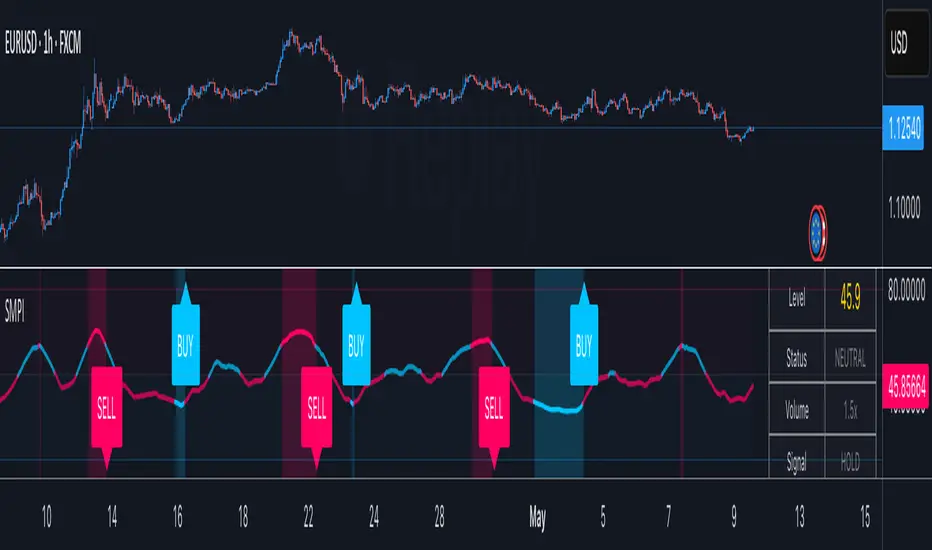
Smart Money Proxy Index Overview The Smart Money Proxy Index (SMPI) is an educational tool that attempts to identify potential institutional-style behavior patterns using publicly available market data. This comprehensive tool combines multiple institutional analysis techniques into a single, easy-to-read 0-100 oscillator. Important Disclaimer This is an educational proxy indicator that analyzes volume and price patterns. It cannot identify actual institutional trading activity and should not be interpreted as tracking real "smart money." Use for educational purposes and combine with other analysis methods. Inspiration & Methodology This indicator is inspired by MAPsignals' Big Money Index (BMI) methodology but uses publicly available price and volume data with original calculations. This is an independent educational interpretation designed to teach smart money concepts to retail traders. What It Analyzes SMPI tracks potential "smart money" activity by combining: Block Trading Detection - Identifies unusual volume surges with significant price impact Money Flow Analysis - Volume-weighted price pressure using Money Flow Index Accumulation/Distribution Patterns - Modified On-Balance Volume signals Institutional Control Proxy - End-of-day positioning and control analysis Key Features – Multi-Component Analysis - Combines 4 different institutional detection methods – BMI-Style 0-100 Scale - Familiar oscillator range with clear extreme levels – Professional Visualization - Dynamic colors, gradient fills, and clean data table – Comprehensive Alerts - Buy/sell signals plus divergence detection – Fully Customizable - Adjust all parameters, colors, and display options – Non-Repainting Signals - All alerts use confirmed data for reliability – Educational Focus - Designed to teach institutional flow concepts How to Interpret Above 80: Potential smart money distribution phase (bearish pressure) Below 20: Potential smart money accumulation phase (bullish opportunity) Signal Generation: Buy signals when crossing above 20, sell signals when crossing below 80 Divergences: Price vs SMPI divergences can signal potential trend changes Volume Confirmation: Higher volume ratios strengthen signal reliability Best Practices Timeframes: Works best on higher timeframes for institutional behavior analysis Confirmation: Combine with other technical analysis tools and market context Volume: Pay attention to volume confirmation in the data table Context: Consider overall market conditions and fundamental factors Risk Management: Not recommended as standalone trading system Customizable Parameters Block Volume Threshold: Sensitivity for unusual volume detection (default: 2.5x average) SMPI Smoothing Period: Index calculation smoothing (default: 25 bars) Extreme Levels: Overbought/oversold thresholds (default: 80/20) Money Flow Length: MFI calculation period (default: 14) Visual Options: Colors, signals, and display preferences Available Alerts Buy Signal: SMPI crosses above oversold level (20) Sell Signal: SMPI crosses below overbought level (80) Extreme Levels: Alerts when reaching overbought/oversold zones Divergence Detection: Bullish and bearish price vs SMPI divergences Educational Purpose & Limitations This indicator is designed as an educational proxy for understanding institutional flow concepts. It analyzes publicly available price and volume data to identify potential smart money behavior patterns. Cannot access actual institutional transaction data Signals may be slower than day-trading indicators (intentionally designed for institutional timeframes) Should be used in conjunction with other analysis methods Past performance does not guarantee future results What Makes This Different Unlike simple volume or momentum indicators, SMPI combines multiple institutional analysis techniques into one comprehensive tool. The multi-component approach provides a more robust view of potential smart money activity.

Indicatore Pine Script®

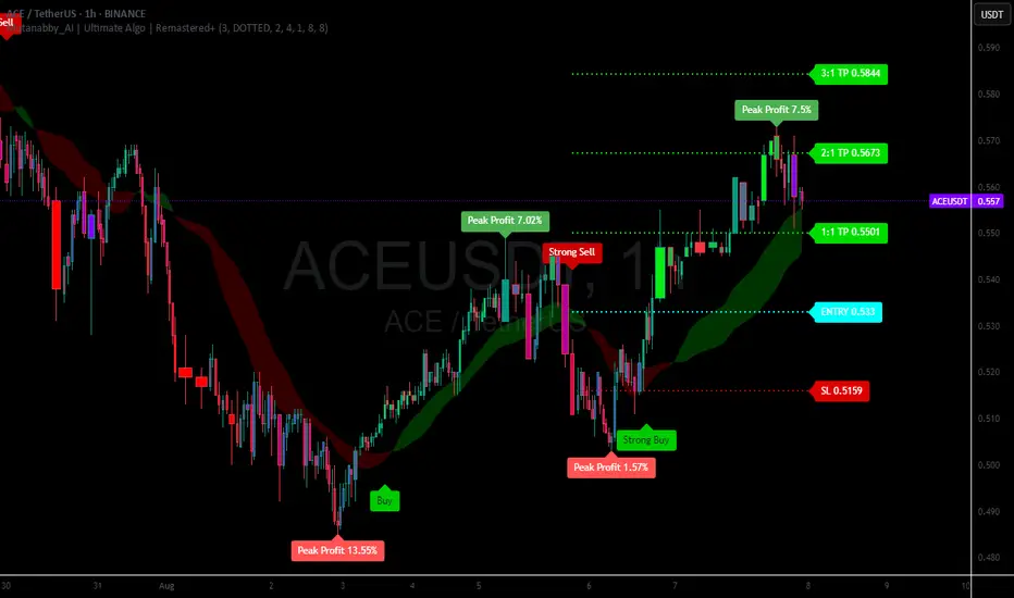
Mutanabby_AI | Ultimate Algo | Remastered+Overview The Mutanabby_AI Ultimate Algo Remastered+ represents a sophisticated trend-following system that combines Supertrend analysis with multiple moving average confirmations. This comprehensive indicator is designed specifically for identifying high-probability trend continuation and reversal opportunities across various market conditions. Core Algorithm Components **Supertrend Foundation**: The primary signal generation relies on a customizable Supertrend indicator with adjustable sensitivity (1-20 range). This adaptive trend-following tool uses Average True Range calculations to establish dynamic support and resistance levels that respond to market volatility. **SMA Confirmation Matrix**: Multiple Simple Moving Averages (SMA 4, 5, 9, 13) provide layered confirmation for signal strength. The algorithm distinguishes between regular signals and "Strong" signals based on SMA 4 vs SMA 5 relationship, offering traders different conviction levels for position sizing. **Trend Ribbon Visualization**: SMA 21 and SMA 34 create a visual trend ribbon that changes color based on their relationship. Green ribbon indicates bullish momentum while red signals bearish conditions, providing immediate visual trend context. **RSI-Based Candle Coloring**: Advanced 61-tier RSI system colors candles with gradient precision from deep red (RSI ≤20) through purple transitions to bright green (RSI ≥79). This visual enhancement helps traders instantly assess momentum strength and overbought/oversold conditions. Signal Generation Logic **Buy Signal Criteria**: - Price crosses above Supertrend line - Close price must be above SMA 9 (trend confirmation) - Signal strength determined by SMA 4 vs SMA 5 relationship - "Strong Buy" when SMA 4 ≥ SMA 5 - Regular "Buy" when SMA 4 < SMA 5 **Sell Signal Criteria**: - Price crosses below Supertrend line - Close price must be below SMA 9 (trend confirmation) - Signal strength based on SMA relationship - "Strong Sell" when SMA 4 ≤ SMA 5 - Regular "Sell" when SMA 4 > SMA 5 Advanced Risk Management System **Automated TP/SL Calculation**: The indicator automatically calculates stop loss and take profit levels using ATR-based measurements. Risk percentage and ATR length are fully customizable, allowing traders to adapt to different market conditions and personal risk tolerance. **Multiple Take Profit Targets**: - 1:1 Risk-Reward ratio for conservative profit taking - 2:1 Risk-Reward for balanced trade management - 3:1 Risk-Reward for maximum profit potential **Visual Risk Display**: All risk management levels appear as both labels and optional trend lines on the chart. Customizable line styles (solid, dashed, dotted) and positioning ensure clear visualization without chart clutter. **Dynamic Level Updates**: Risk levels automatically recalculate with each new signal, maintaining current market relevance throughout position lifecycles. Visual Enhancement Features **Customizable Display Options**: Toggle trend ribbon, TP/SL levels, and risk lines independently. Decimal precision adjustments (1-8 decimal places) accommodate different instrument price formats and personal preferences. **Professional Label System**: Clean, informative labels show entry points, stop losses, and take profit targets with precise price levels. Labels automatically position themselves for optimal chart readability. **Color-Coded Momentum**: The gradient RSI candle coloring system provides instant visual feedback on momentum strength, helping traders assess market energy and potential reversal zones. Implementation Strategy **Timeframe Optimization**: The algorithm performs effectively across multiple timeframes, with higher timeframes (4H, Daily) providing more reliable signals for swing trading. Lower timeframes work well for day trading with appropriate risk adjustments. **Sensitivity Adjustment**: Lower sensitivity values (1-5) generate fewer but higher-quality signals, ideal for conservative approaches. Higher sensitivity (15-20) increases signal frequency for active trading styles. **Risk Management Integration**: Use the automated risk calculations as baseline parameters, adjusting risk percentage based on account size and market conditions. The 1:1, 2:1, 3:1 targets enable systematic profit-taking strategies. Market Application **Trend Following Excellence**: Primary strength lies in capturing significant trend movements through the Supertrend foundation with SMA confirmation. The dual-layer approach reduces false signals common in single-indicator systems. **Momentum Assessment**: RSI-based candle coloring provides immediate momentum context, helping traders assess signal strength and potential continuation probability. **Range Detection**: The trend ribbon helps identify ranging conditions when SMA 21 and SMA 34 converge, alerting traders to potential breakout opportunities. Performance Optimization **Signal Quality**: The requirement for both Supertrend crossover AND SMA 9 confirmation significantly improves signal reliability compared to basic trend-following approaches. **Visual Clarity**: The comprehensive visual system enables rapid market assessment without complex calculations, ideal for traders managing multiple instruments. **Adaptability**: Extensive customization options allow fine-tuning for specific markets, trading styles, and risk preferences while maintaining the core algorithm integrity. ## Non-Repainting Design **Educational Note**: This indicator uses standard TradingView functions (Supertrend, SMA, RSI) with normal behavior patterns. Real-time updates on current candles are expected and standard across all technical indicators. Historical signals on closed candles remain fixed and unchanged, ensuring reliable backtesting and analysis. **Signal Confirmation**: Final signals are confirmed only when candles close, following standard technical analysis principles. The algorithm provides clear distinction between developing signals and confirmed entries. Technical Specifications **Supertrend Parameters**: Default sensitivity of 4 with ATR length of 11 provides balanced signal generation. Sensitivity range from 1-20 allows adaptation to different market volatilities and trading preferences. **Moving Average Configuration**: SMA periods of 8, 9, and 13 create multi-layered trend confirmation, while SMA 21 and 34 form the visual trend ribbon for broader market context. **Risk Management**: ATR-based calculations with customizable risk percentage ensure dynamic adaptation to market volatility while maintaining consistent risk exposure principles. Recommended Settings **Conservative Approach**: Sensitivity 4-5, RSI length 14, higher timeframes (4H, Daily) for swing trading with maximum signal reliability. **Active Trading**: Sensitivity 6-8, RSI length 8-10, intermediate timeframes (1H) for balanced signal frequency and quality. **Scalping Setup**: Sensitivity 10-15, RSI length 5-8, lower timeframes (15-30min) with enhanced risk management protocols. ## Conclusion The Mutanabby_AI Ultimate Algo Remastered+ combines proven trend-following principles with modern visual enhancements and comprehensive risk management. The algorithm's strength lies in its multi-layered confirmation approach and automated risk calculations, providing both novice and experienced traders with clear signals and systematic trade management. Success with this system requires understanding the relationship between signal strength indicators and adapting sensitivity settings to match current market conditions. The comprehensive visual feedback system enables rapid decision-making while the automated risk management ensures consistent trade parameters. Practice with different sensitivity settings and timeframes to optimize performance for your specific trading style and risk tolerance. The algorithm's systematic approach provides an excellent framework for disciplined trend-following strategies across various market environments.

Indicatore Pine Script®

di Mutanabby_AI

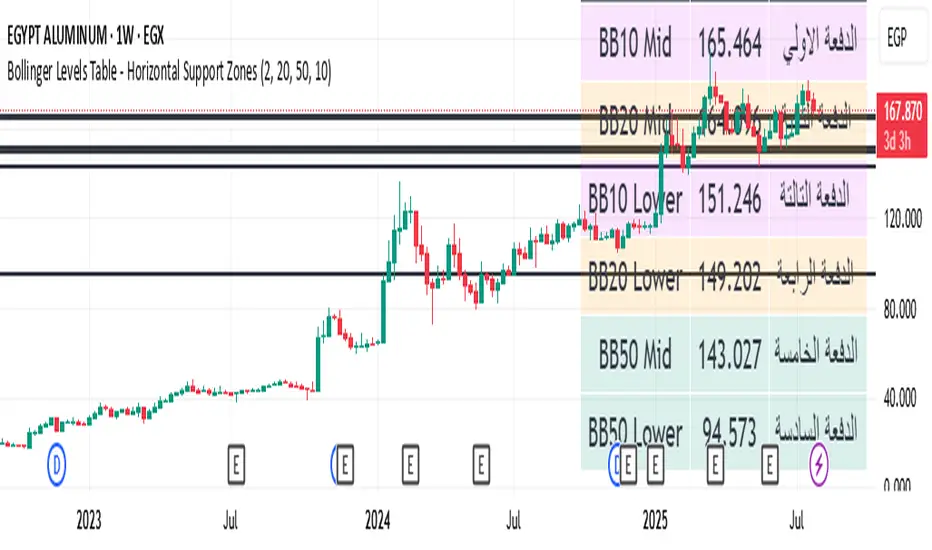
Bollinger Levels Table - Horizontal Support Zones Bollinger Levels Table - Horizontal Support Zones Indicator (with Customizable Options) The "Bollinger Levels Table - Horizontal Support Zones" indicator is a comprehensive tool designed to help you identify potential support areas on your chart using moving averages and Bollinger Bands. The indicator displays an organized table of key price levels and draws horizontal lines on the chart, providing clear visibility of potential support zones. What Does This Indicator Do? This indicator aims to simplify support analysis by consolidating and displaying significant price levels derived from three different Bollinger Band settings: BB10, BB20, and BB50. It calculates both the Mid-line (Basis) and the Lower Band for each of these settings. Furthermore, the indicator automatically arranges these levels from highest to lowest in an easy-to-read table, assigning a "Payment" label to each level. These "Payments" are simply labels to help you track the levels in descending order. How Does This Indicator Work? Bollinger Band Calculations: The indicator uses the standard Bollinger Band formula: Mid-line (Basis): A Simple Moving Average (SMA) of the closing price over a specified period. Standard Deviation (Dev): The standard deviation of the closing price over the same period, multiplied by a Multiplier. Lower Band: The Mid-line minus the Standard Deviation. These calculations are applied to three different periods: 10, 20, and 50, providing a variety of potential support levels based on different timeframes. You can adjust the values for these lengths (10, 20, 50) and the Multiplier through the indicator's settings. Table Construction: A dynamic table is created on the chart (which can be positioned in the top or bottom right corner based on the current price's position). This table displays: Indicator: The name of the Bollinger Band level (e.g., BB10 Mid, BB20 Lower). Price: The exact price value of that level. Payments: A label indicating the level's order in the table. Level Ordering: All calculated levels are dynamically sorted from highest to lowest to present them in a logical order within the table. Horizontal Line Plotting: Horizontal lines are drawn on the chart for each selected level, providing a visual representation of the potential support areas. These lines are colored black and have a consistent width for easy identification. How to Use This Indicator: This indicator is intended to provide potential entry points or accumulation zones for trades, especially for traders employing Dollar-Cost Averaging (DCA) strategies or building positions in stages. The levels displayed in the table and on the chart can represent potential support levels where one might consider initiating or adding to a position. In the indicator's settings, you'll find important options: Multiplier: Controls the width of the Bollinger Bands (default 2.0). BB Lengths: Allows you to adjust the periods for the moving averages (default 20, 50, 10). Visible Levels: This is the new feature! Here, you can select which levels you wish to see in the table and on the chart. Simply check or uncheck the boxes next to each level (BB10 Mid, BB10 Lower, and so on) to customize the indicator's display according to your strategy and needs. Underlying Concepts: This indicator is based on the principle that Bollinger Bands can act as dynamic support and resistance zones. Mid-line (SMA): Often functions as a medium-term support or resistance. Lower Band: Typically indicates that the price is relatively low and may find support, making it a potential area for buying or starting to build a position. By combining different Bollinger Band timeframes (10, 20, 50), the indicator gives you a multi-timeframe perspective on support areas, helping you identify the most relevant levels for your strategy. Note: While the indicator provides "Payments" for the levels, this is purely a sequential labeling within the table to assist your position-building strategy. There is no actual payment functionality associated with this indicator.

Indicatore Pine Script®

di khalidaladdin1990

Candle Channel █ OVERVIEW The "Candle Channel" indicator is a versatile technical analysis tool that plots a price channel based on the Simple Moving Average (SMA) of candlestick midpoints. The channel bands, calculated based on candlestick volatility, form dynamic support and resistance levels that adapt to price movements. The script generates signals for reversals from the bands and SMA breakouts, making it useful for both short-term and long-term traders. By adjusting the SMA length, the channel can vary in nature—from a wide channel encapsulating price movement to narrower support/resistance or trend-following bands. The channel width can be further customized using a scaling parameter, allowing adaptation to different trading styles and markets. █ MECHANISM Band Calculation The indicator is based on the following calculations: Candlestick Midpoint: Calculated as the arithmetic average of the candle’s high and low prices: (high + low) / 2. Simple Moving Average (SMA): The average of candlestick midpoints over a specified length (default: 20 candles), forming the channel’s centerline. Average Candle Height: Calculated as the average difference between the high and low prices (high - low) over the same SMA length, serving as a measure of market volatility. Band Scaling: The user specifies a percentage of the average candle height (default: 200%), which is multiplied by the average height to create an offset. The upper band is SMA + offset, and the lower band is SMA - offset.Example: For an average candle height of 10 points and 200% scaling, the offset is 20 points, meaning the bands are ±20 points from the SMA. Channel Characteristics: The SMA length determines the channel’s dynamics. Shorter SMA values (10–30) create a wide channel that contains price movement, ideal for scalping or short-term trading. Longer SMA values (above 30, e.g., 50–100) transform the channel into narrower support/resistance or trend-following bands, suitable for longer-term analysis. Band scaling further adjusts the channel width to match market volatility. Signals Reversal from Bands: Signals are generated when the price closes outside the band (above the upper or below the lower) and then returns to the channel, indicating a potential trend reversal. SMA Breakout: Signals are generated when the price crosses the SMA upward (bullish signal) or downward (bearish signal), suggesting potential trend changes. Visualization Centerline: The SMA of candlestick midpoints, displayed as a thin line. Channel Bands: Upper and lower channel boundaries, with customizable colors. Fill: Options include a gradient (smooth color transition between bands) or solid color. The fill can also be disabled for greater clarity. █ FEATURES AND SETTINGS SMA Length: Determines the moving average period (default: 20). Values of 10–30 are suitable for a wide channel containing price movement, ideal for short-term timeframes. Longer values (e.g., 50–100) create narrower support/resistance or trend-following bands, better suited for higher timeframes. Band Scaling: Percentage of the average candle height (default: 200%). Adjusts the channel width to match market volatility—smaller values (e.g., 50–100%) for narrower bands, larger values (e.g., 200–300%) for wider channels. Fill Type: Gradient, solid, or no fill, allowing customization to user preferences. Colors: Options to change the colors of bands, fill, and signals for better readability. Signals: Options to enable/disable reversal signals from bands and SMA breakout signals. █ HOW TO USE Add the script to your chart in TradingView by clicking "Add to Chart" in the Pine Editor. Adjust input parameters in the script settings: SMA Length: Set to 10–30 for a wide channel containing price movement, suitable for scalping or short-term trading. Set above 30 (e.g., 50–100) for narrower support/resistance or trend-following bands. Band Scaling: Adjust the channel width to market volatility. Smaller values (50–100%) for tighter support/resistance bands, larger values (200–300%) for wider channels containing price movement. Fill Type and Colors: Choose a gradient for aesthetics or a solid fill for clarity. Analyze signals: Reversal Signals: Triangles above (bearish) or below (bullish) candles indicate potential reversal points. SMA Breakout Signals: Circles above (bearish) or below (bullish) candles indicate trend changes. Test the indicator on different instruments and timeframes to find optimal settings for your trading style. █ LIMITATIONS The indicator may generate false signals in highly volatile or consolidating markets. On low-liquidity charts (e.g., exotic currency pairs), the bands may be less reliable. Effectiveness depends on properly matching parameters to the market and timeframe.

Indicatore Pine Script®

di Uncle_the_shooter

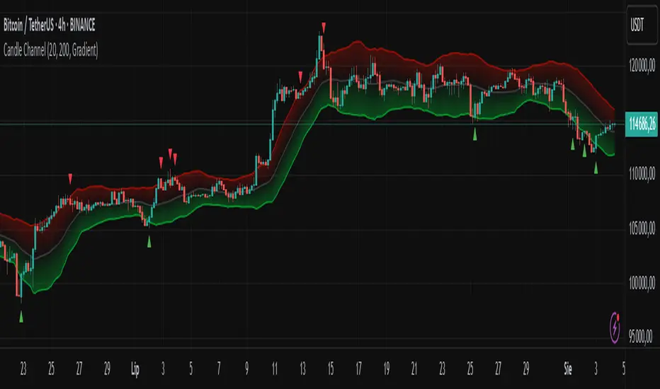
EMA Trend Confirmation with Alerts 此脚本是基于EMA 200周期 50周期 20周期加以合并并进行改进的一个脚本指标，主要作用是用于观察趋势走向，其中有上升下降和震荡趋势，经过多数测试，此指标适用于短线交易，推荐周期为20或15，大周期和长线交易详见RSI+EMA结合指标 This script is an improved script indicator based on the EMA 200 period, 50 period, and 20 period. Its main function is to observe the trend direction, including up, down, and oscillating trends. After many tests, this indicator is suitable for short-term trading, and the recommended period is 20 or 15. For large-cycle and long-term trading, please refer to the RSI+EMA combination indicator.

Indicatore Pine Script®

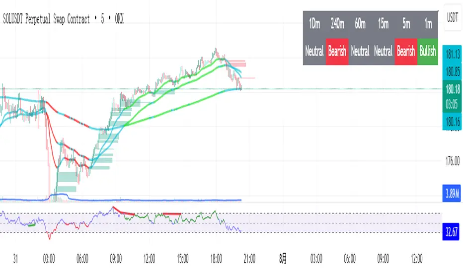
9:45am NIFTY TRADING Time Frame: 15 Minutes | Reference Candle Time: 9:45 AM IST | Valid Trading Window: 3 Hours 📌 Introduction This document outlines a structured trading strategy for NIFTY & BANKNIFTY Options based on a 15-minute timeframe with a 9:45 AM IST reference candle. The strategy incorporates technical indicators, probability analysis, and strict trading rules to optimize entries and exits. 📊 Core Features 1. Reference Time Trading System 9:45 AM IST Candle acts as the reference for the day. All signals (Buy/Sell/Reversal) are generated based on price action relative to this candle. The valid trading window is 3 hours after the reference candle. 2. Signal Generation Logic Signal Condition Buy (B) Price breaks above reference candle high with confirmation Sell (S) Price breaks below reference candle low with confirmation Reversal (R) Early trend reversal signal (requires strict confirmation) 3. Probability Analysis System The strategy calculates Win Probability (%) using 4 components: Component Weight Calculation Body Win Probability 30% Based on candle body strength (body % of total range) Volume Win Probability 30% Current volume vs. average volume strength Trend Win Probability 40% EMA crossover + RSI momentum alignment Composite Probability - Weighted average of all 3 components Probability Color Coding: 🟢 Green (High Probability): ≥70% 🟠 Orange (Medium Probability): 50-69% 🔴 Red (Low Probability): <50% 4. Timeframe Enforcement Strictly 15-minute charts only (no other timeframes allowed). System auto-disables signals if the wrong timeframe is selected. 📈 Technical Analysis Components 1. EMA System (Trend Analysis) Short EMA (9) – Fast trend indicator Middle EMA (20) – Intermediate trend Long EMA (50) – Long-term trend confirmation Rules: Buy Signal: Price > 9 EMA > 20 EMA > 50 EMA (Bullish trend) Sell Signal: Price < 9 EMA < 20 EMA < 50 EMA (Bearish trend) 2. Multi-Timeframe RSI (Momentum) 5M, 15M, 1H, 4H, Daily RSI values are compared for divergence/confluence. Overbought (≥70) / Oversold (≤30) conditions help in reversal signals. 3. Volume Analysis Volume Strength (%) = (Current Volume / Avg. Volume) × 100 Strong Volume (>120% Avg.) confirms breakout/breakdown. 4. Body Percentage (Candle Strength) Body % = (Close - Open) / (High - Low) × 100 Strong Bullish Candle: Body > 60% Strong Bearish Candle: Body < 40% 📊 Visual Elements 1. Information Tables Reference Data Table (9:45 AM Candle High/Low/Close) RSI Values Table (5M, 15M, 1H, 4H, Daily) Signal Legend (Buy/Sell/Reversal indicators) 2. Chart Overlays Reference Lines (9:45 AM High & Low) EMA Lines (9, 20, 50) Signal Labels (B, S, R) 3. Color Coding High Probability (Green) Medium Probability (Orange) Low Probability (Red) ⚠️ Important Usage Guidelines ✅ Best Practices: Trade only within the 3-hour window (9:45 AM - 12:45 PM IST). Wait for confirmation (closing above/below reference candle). Use probability score to filter high-confidence trades. ❌ Avoid: Trading outside the 15-minute timeframe. Ignoring volume & RSI divergence. Overtrading – Stick to 1-2 high-probability setups per day. 🎯 Conclusion This NIFTY Trading Strategy is optimized for 15-minute charts with a 9:45 AM IST reference candle. It combines EMA trends, RSI momentum, volume analysis, and probability scoring to generate high-confidence signals. 🚀 Key Takeaways: ✔ Reference candle defines the day’s bias. ✔ Probability system filters best trades. ✔ Strict 15M timeframe ensures consistency. Happy Trading! 📈💰

Indicatore Pine Script®

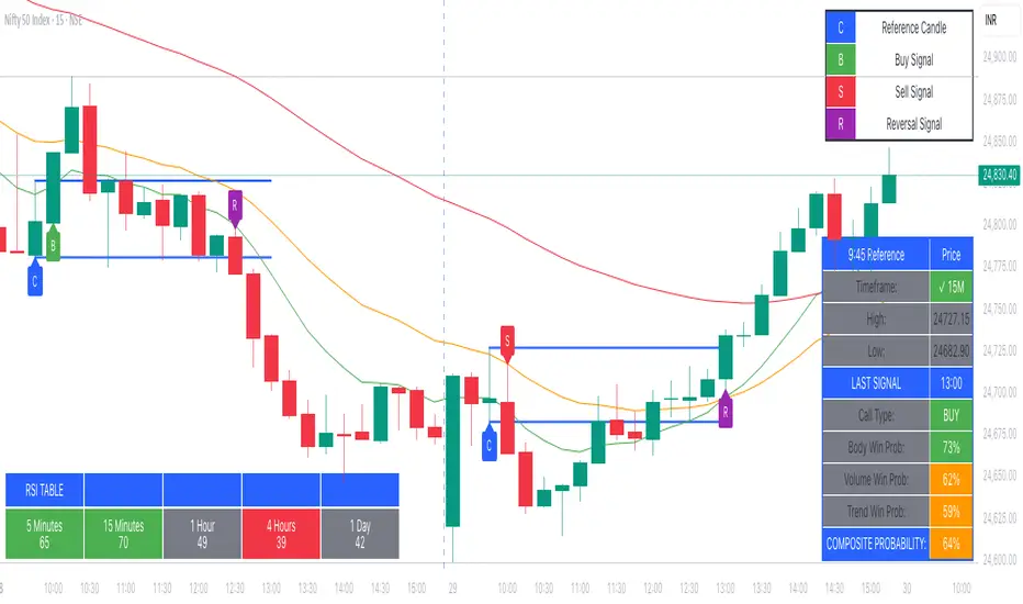
EMA+ATR Band MTF Trend Entry This is a Multi-Timeframe Trend Trading indicator strategy adapted from Sahil Rohmehtra’s Mentorship programme. The trading decision is made by first accessing the trend in higher timeframe (say Monthly) by using TWO EMAs. If the faster EMA (say 20 period) is above Slower EMA (say 50 period) and the price is above slower EMA then the trend is suitable for buyers. Similarly if faster EMA is below slow EMA and the price is below that then trend is suitable for sellers. Once we access the trend in the higher timeframe we move to the lower timeframe (say Weekly) and access the 5-period RSI value. If RSI is below 30 then we can prepare for possible buy entry in lower (Daily) timeframe if entry conditions are met in daily timeframe. Similarly sell bias can be initiated when the higher timeframe EMA trend is down, daily RSI is above 70 and sell entry condition is met in daily timeframe. The RSI thresholds can be changed by the user. Once we identified the RSI bias then wait for the confirmation candle in the lower timeframe (say 1 hour). In the entry timeframe we plot a band of 20 EMA of LOWs ± 1 ATR lines. Here,we wait for a candle to close above the 20 EMA of LOWs + 1 ATR for a buy signal with an increase in On Balance Volume (OBV) value. Similarly for sell signal we should get a candle close below the 20 EMA of LOWs - 1 ATR with corresponding change in OBV. This candle is the signal candle. Once we get a Buy or Sell signal the corresponding stop loss is the nearest LOW - 1 ATR or HIGH + 1 ATR. The ATR scaling may be changed by the user. Now if another candle closes above the high of the buy signal candle then enter on buy. If the low of the buy signal candle is broken then it is a potential short-term sell entry. Similarly if another candle closes below the sell signal candle then enter short and if there is a close above high of the signal candle then it is a potential buy entry.

Indicatore Pine Script®

di librantrader

Aggiornato

Stochastic Ribbon & EMAs Here's a comprehensive description for publishing your indicator: --- # **Stochastic Ribbon & EMAs** A clean and powerful trading indicator that combines **Stochastic Support/Resistance levels** with **Essential Moving Averages** for comprehensive market analysis. ## **📊 What It Does** This indicator provides **7 key reference lines** on your chart: - **3 Stochastic levels** (20%, 50%, 80%) - Dynamic support/resistance zones - **4 Essential EMAs** (20, 50, 100, 200) - Trend direction and momentum ## **🎯 Key Features** ### **Stochastic Ribbon (3 Yellow Lines)** - **80% Line**: Dynamic resistance level - potential selling zone - **50% Line**: Market equilibrium - trend direction reference - **20% Line**: Dynamic support level - potential buying zone - **Default 50-period lookback** for stable, reliable levels - **All lines in yellow** for clean, consistent visualization ### **Essential EMAs (4 Colored Lines)** - **20 EMA** (Purple): Short-term trend and entry timing - **50 EMA** (Dark Cyan): Medium-term trend direction - **100 EMA** (Rosy Brown): Long-term trend confirmation - **200 EMA** (Brown): Major trend and institutional levels ## **📈 How to Use** ### **For Support & Resistance:** - **Above 80% line**: Look for selling opportunities (overbought zone) - **Between 50-80%**: Bullish bias, pullbacks to 50% line for entries - **Around 50% line**: Key equilibrium - watch for direction - **Between 20-50%**: Bearish bias, bounces to 50% line for exits - **Below 20% line**: Look for buying opportunities (oversold zone) ### **For Trend Analysis:** - **EMA Stack Order**: Higher timeframe EMAs above lower = uptrend - **Price above all EMAs**: Strong bullish momentum - **Price below all EMAs**: Strong bearish momentum - **EMA as dynamic support/resistance**: Bounces and rejections ### **For Entry Signals:** - **Confluence zones**: Where Stochastic levels meet EMA levels - **Breakouts**: Price breaking through multiple levels simultaneously - **Reversals**: Price rejection at extreme Stochastic levels with EMA confirmation ## **⚙️ Settings** ### **Stochastic Ribbon** - **Show/Hide**: Toggle the 3 Stochastic lines - **Length**: Period for high/low calculation (default: 50) - **Start**: Multiplier for calculation (default: 1) ### **EMAs** - **Individual toggles**: Show/hide each EMA separately - **Custom periods**: Adjust each EMA length (defaults: 20, 50, 100, 200) - **Custom colors**: Personalize each EMA color ## **🚀 Why This Indicator?** ✅ **Clean & Simple**: No cluttered charts - just essential levels ✅ **Multi-Timeframe**: Works on all timeframes from 1m to 1W ✅ **Versatile**: Suitable for scalping, day trading, and swing trading ✅ **Low Lag**: Dynamic levels that adapt to current market conditions ✅ **Proven Components**: Combines two well-established technical concepts ✅ **Customizable**: Adjust all parameters to fit your trading style ## **💡 Pro Tips** - **Use multiple timeframes**: Check higher timeframe alignment for stronger signals - **Combine with volume**: Look for volume confirmation at key levels - **Watch for confluences**: Best signals occur where multiple levels align - **Respect the 50% line**: Often acts as the most important level for trend direction ## **📋 Technical Details** - **Version**: Pine Script v5 - **Overlay**: Yes (displays on main price chart) - **Plots**: 7 total (well within Pine Script limits) - **Performance**: Optimized for fast loading and smooth operation --- **Perfect for traders who want clear, actionable levels without chart clutter. Whether you're a beginner learning support/resistance or an experienced trader looking for clean reference points, this indicator delivers exactly what you need.**

Indicatore Pine Script®

di insomniac_vampire

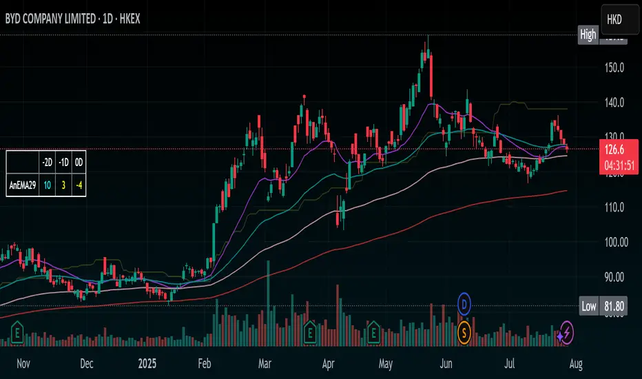
TZanalyser TZanalyser (Trend Zone Monitor With Trend Strength, Volume Focus And -Events Markers) Before I used TrendZones to manage my portfolio I used Fibonacci Zone Oscillator as my favorite in the sub panel, accompanied with another subpanel indicator which I never published called IncliValue and also REVE Cohorts. TZanalyser inherits Ideas and code from all three of them: The visual and the idea of using a channel as the basis for an oscillator depicted as a histogram, is taken from the FibZone Oscillator. The idea of providing a number to evaluate the trend is taken from IncliValue. The idea to create a horizontal line which indicates high and low volume focus completed with markers for volume events, is taken from REVE-cohorts. These ideas are combined in one sleek visual called TZanalyser. TZ stand for TrendZones, because the histogram is based on it. The histogram. Depicted is the distance of the price from COG as percent. The distance between Upper Curve and Lower Curve is used as 100%. The values may reach between 300 and -300. The colors indicate in which zone the candle lives, blue in the blue zone, green in the green zone etc. Despite the absence of a gray zone, there are gray bars. These depict candles that wrap around COG. Because hl2 is used as price, some gray bars point up and others down. The orange and red bars point down because the orange and red downtrend zones are below COG. Use of the histogram. Sometimes I need to create a list of stocks which are in uptrend in monthly, weekly and daily charts from the stocks I follow in my universe. This job is done fast and easy by looking at the last bar of the histogram. The histogram also gives a quick evaluation of how the stock fared in the past. The number. Suppose I need to allocate some money to another stock, selected a few, looked into news and gurus and they look equally good. Then it is nice to be able to find out which has the best charts. Which one has the strongest uptrend. For this purpose this number can be consulted, because it indicates somehow the strength of the trend. It is an integer between 20 and -20, the closer to 20 the stronger the uptrend, closer to -20 indicates a stronger downtrend. The color of the background is the same as the last column of the histogram. Volume focus and events The horizontal lines depict volume focus, the line below the focus that comes with the uptrend columns pointing up, the one above the focus for the downtrend columns pointing down. Thes line have tree colors: maroon for high volume focus, green for normal volume and gray for low volume situations. Between the lines and the histogram triangles appear at volume events, a green triangle when the candle comes with high volume, i.e. 120-200 percent of normal, maroon when extreme volume, i.e. more than 200 percent of normal. The direction of these triangles is that of the histogram, i.e. when the price is higher, direction is up and vice versa. Take care and have fun.

Indicatore Pine Script®

Aggiornato

Pivot Channel Levels Pivot Channel Levels Indicator Description “Pivot Channel Levels” is an advanced technical analysis tool that identifies key price pivots (highs and lows) and creates dynamic support and resistance levels based on the wicks of candles at these points (or bodies if wicks are minimal). The indicator analyzes the volume at the time of a pivot’s formation, displaying its value and percentage change relative to the volume’s simple moving average (SMA). It does not generate buy/sell signals but provides a clear visualization of market structure, helping traders identify potential price reaction zones and assess the strength of market movements. Why Are Wicks Important? Candle wicks at price pivots indicate significant market reactions in key areas. Depending on the context, they may signal rejection, testing, or absorption of a support or resistance level. Long wicks often appear where large players are active, and the marked zones are frequently retested. The indicator allows for quick identification and observation of their impact on future price action. Why Use It? - Precise Support and Resistance Levels: The indicator draws price channels based on candle wicks at pivots (or bodies if wicks are absent), enabling better identification of zones where price may react. - Volume Analysis: It shows how the volume at a pivot differs from the average, indicating potential activity by large players or key market moments. - Visual Clarity: Colored lines, channel fills, and clear labels facilitate quick chart analysis, even on short timeframes. - Flexibility: Adjustable pivot length, volume average, and label colors allow customization to various trading strategies. How It Works - Pivot Detection: Automatically identifies local highs and lows based on the “Pivot Length” parameter (default: 20 candles). This means a pivot appears on the chart with a 20-candle delay. Reducing this value allows faster pivot detection (after fewer candles), increasing their number but potentially generating more noise. - Channel Creation: Draws support and resistance levels based on the wicks of candles at pivot points (or bodies if wicks are minimal) with a delay to confirm zones. A pivot channel is drawn until the next pivot is identified, but if not previously broken, it remains valid as active support or resistance. - Volume Analysis: Displays the volume at the pivot’s formation and its percentage change relative to the volume’s SMA. - Visualization: Pivot and channel levels are shown as lines with fills, and labels display volume and its deviation from the average. Trading Applications - Swing Trading: Use pivot levels and channels to identify price reversal points or consolidation zones. - Scalping: Monitor price reactions to channels on short timeframes, especially with high volume. - Faster Pivot Identification: Switch to a lower timeframe (e.g., from H1 to M15) to identify pivots more quickly, allowing earlier reactions to price changes. - Market Context Analysis: High volume at pivots may indicate significant levels likely to be retested. - Combining with Other Tools: The indicator pairs well with Fibonacci retracement, supply/demand zones, or oscillators like RSI. Settings and Customization - Pivot Length: Determines how many candles back and forward are analyzed to detect pivots (default: 20). A smaller value increases sensitivity, a larger one enhances stability. - Volume Average: Length of the SMA for volume (default: 20). Adjust to better reflect market characteristics. - Label Colors: Choose colors for bullish and bearish pivot labels to match your chart style. Usage Examples - Identifying Key Zones: If the price approaches a pivot level with high volume (e.g., +50% relative to SMA), it may signal strong support or resistance. - Breakout Confirmation: A channel breakout with high volume can indicate trend continuation. - Price Reaction Analysis: Long wicks at pivots with high volume may signal level rejection by large players. Notes for Users - The indicator performs best on highly liquid markets (e.g., Forex, indices, cryptocurrencies). - On short timeframes (e.g., M1, M5), it may generate more noise—adjust “Pivot Length” to suit your needs. - Consider combining with other indicators to confirm signals derived from pivot and volume analysis.

Indicatore Pine Script®

di Uncle_the_shooter

Active PMI Support/Resistance Levels [EdgeTerminal]The PMI Support & Resistance indicator revolutionizes traditional technical analysis by using Pointwise Mutual Information (PMI) - a statistical measure from information theory - to objectively identify support and resistance levels. Unlike conventional methods that rely on visual pattern recognition, this indicator provides mathematically rigorous, quantifiable evidence of price levels where significant market activity occurs. - The Mathematical Foundation: Pointwise Mutual Information Pointwise Mutual Information measures how much more likely two events are to occur together compared to if they were statistically independent. In our context: Event A: Volume spikes occurring (high trading activity) Event B: Price being at specific levels The PMI formula calculates: PMI = log(P(A,B) / (P(A) × P(B))) Where: P(A,B) = Probability of volume spikes occurring at specific price levels P(A) = Probability of volume spikes occurring anywhere P(B) = Probability of price being at specific levels High PMI scores indicate that volume spikes and certain price levels co-occur much more frequently than random chance would predict, revealing genuine support and resistance zones. - Why PMI Outperforms Traditional Methods Subjective interpretation: What one trader sees as significant, another might ignore Confirmation bias: Tendency to see patterns that confirm existing beliefs Inconsistent criteria: No standardized definition of "significant" volume or price action Static analysis: Doesn't adapt to changing market conditions No strength measurement: Can't quantify how "strong" a level truly is PMI Advantages: ✅ Objective & Quantifiable: Mathematical proof of significance, not visual guesswork ✅ Statistical Rigor: Levels backed by information theory and probability ✅ Strength Scoring: PMI scores rank levels by statistical significance ✅ Adaptive: Automatically adjusts to different market volatility regimes ✅ Eliminates Bias: Computer-calculated, removing human interpretation errors ✅ Market Structure Aware: Reveals the underlying order flow concentrations - How It Works Data Processing Pipeline: Volume Analysis: Identifies volume spikes using configurable thresholds Price Binning: Divides price range into discrete levels for analysis Co-occurrence Calculation: Measures how often volume spikes happen at each price level PMI Computation: Calculates statistical significance for each price level Level Filtering: Shows only levels exceeding minimum PMI thresholds Dynamic Updates: Refreshes levels periodically while maintaining historical traces Visual System: Current Levels: Bright, thick lines with PMI scores - your actionable levels Historical Traces: Faded previous levels showing market structure evolution Strength Tiers: Line styles indicate PMI strength (solid/dashed/dotted) Color Coding: Green for support, red for resistance Info Table: Real-time display of strongest levels with scores - Indicator Settings: Core Parameters Lookback Period (Default: 200) Lower (50-100): More responsive to recent price action, catches short-term levels Higher (300-500): Focuses on major historical levels, more stable but less responsive Best for: Day trading (100-150), Swing trading (200-300), Position trading (400-500) Volume Spike Threshold (Default: 1.5) Lower (1.2-1.4): More sensitive, catches smaller volume increases, more levels detected Higher (2.0-3.0): Only major volume surges count, fewer but stronger signals Market dependent: High-volume stocks may need higher thresholds (2.0+), low-volume stocks lower (1.2-1.3) Price Bins (Default: 50) Lower (20-30): Broader price zones, less precise but captures wider areas Higher (70-100): More granular levels, precise but may be overly specific Volatility dependent: High volatility assets benefit from more bins (70+) Minimum PMI Score (Default: 0.5) Lower (0.2-0.4): Shows more levels including weaker ones, comprehensive view Higher (1.0-2.0): Only statistically strong levels, cleaner chart Progressive filtering: Start with 0.5, increase if too cluttered Max Levels to Show (Default: 8) Fewer (3-5): Clean chart focusing on strongest levels only More (10-15): Comprehensive view but may clutter chart Strategy dependent: Scalpers prefer fewer (3-5), swing traders more (8-12) Historical Tracking Settings Update Frequency (Default: 20 bars) Lower (5-10): More frequent updates, captures rapid market changes Higher (50-100): Less frequent updates, focuses on major structural shifts Timeframe scaling: 1-minute charts need lower frequency (5-10), daily charts higher (50+) Show Historical Levels (Default: True) Enables the "breadcrumb trail" effect showing evolution of support/resistance Disable for cleaner charts focusing only on current levels Max Historical Marks (Default: 50) Lower (20-30): Less memory usage, shorter history Higher (100-200): Longer historical context but more resource intensive Fade Strength (Default: 0.8) Lower (0.5-0.6): Historical levels more visible Higher (0.9-0.95): Historical levels very subtle Visual Settings Support/Resistance Colors: Choose colors that contrast well with your chart theme Line Width: Thicker lines (3-4) for better visibility on busy charts Show PMI Scores: Toggle labels showing statistical strength Label Size: Adjust based on screen resolution and chart zoom level - Most Effective Usage Strategies For Day Trading: Setup: Lookback 100-150, Volume Threshold 1.8-2.2, Update Frequency 10-15 Use PMI levels as bounce/rejection points for scalp entries Higher PMI scores (>1.5) offer better probability setups Watch for volume spike confirmations at levels For Swing Trading: Setup: Lookback 200-300, Volume Threshold 1.5-2.0, Update Frequency 20-30 Enter on pullbacks to high PMI support levels Target next resistance level with PMI score >1.0 Hold through minor levels, exit at major PMI levels For Position Trading: Setup: Lookback 400-500, Volume Threshold 2.0+, Update Frequency 50+ Focus on PMI scores >2.0 for major structural levels Use for portfolio entry/exit decisions Combine with fundamental analysis for timing - Trading Applications: Entry Strategies: PMI Bounce Trades Price approaches high PMI support level (>1.0) Wait for volume spike confirmation (orange triangles) Enter long on bullish price action at the level Stop loss just below the PMI level Target: Next PMI resistance level PMI Breakout Trades Price consolidates near high PMI level Volume increases (watch for orange triangles) Enter on decisive break with volume Previous resistance becomes new support Target: Next major PMI level PMI Rejection Trades Price approaches PMI resistance with momentum Watch for rejection signals and volume spikes Enter short on failure to break through Stop above the PMI level Target: Next PMI support level Risk Management: Stop Loss Placement Place stops 0.1-0.5% beyond PMI levels (adjust for volatility) Higher PMI scores warrant tighter stops Use ATR-based stops for volatile assets Position Sizing Larger positions at PMI levels >2.0 (highest conviction) Smaller positions at PMI levels 0.5-1.0 (lower conviction) Scale out at multiple PMI targets - Key Warning Signs & What to Watch For Red Flags: 🚨 Very Low PMI Scores (<0.3): Weak statistical significance, avoid trading 🚨 No Volume Confirmation: PMI level without recent volume spikes may be stale 🚨 Overcrowded Levels: Too many levels close together suggests poor parameter tuning 🚨 Outdated Levels: Historical traces are reference only, not tradeable Optimization Tips: ✅ Regular Recalibration: Adjust parameters monthly based on market regime changes ✅ Volume Context: Always check for recent volume activity at PMI levels ✅ Multiple Timeframes: Confirm PMI levels across different timeframes ✅ Market Conditions: Higher thresholds during high volatility periods Interpreting PMI Scores PMI Score Ranges: 0.5-1.0: Moderate statistical significance, proceed with caution 1.0-1.5: Good significance, reliable for most trading strategies 1.5-2.0: Strong significance, high-confidence trade setups 2.0+: Very strong significance, institutional-grade levels Historical Context: The historical trace system shows how support and resistance evolve over time. When current levels align with multiple historical traces, it indicates persistent market memory at those prices, significantly increasing the level's reliability.

Indicatore Pine Script®

di EdgeTerminal

Staccked SMA - Regime Switching & Persistance Statistics This indicator is designed to identify the prevailing market regime by analyzing the behavior of a "stack" of Simple Moving Averages (SMAs). It helps you understand whether the market is currently trending, mean-reverting, or moving randomly. Core Concept: SMA Correlation At its heart, the indicator examines the relationship between a set of nine SMAs with different lengths (3, 5, 8, 13, 21, 34, 55, 89, 144) and the lengths themselves. In a strong trending market (either up or down), the SMAs will be neatly "stacked" in order of their length. The shortest SMA will be furthest from the longest SMA, creating a strong, almost linear visual pattern. When we measure the statistical correlation between the SMA values and their corresponding lengths, we get a value close to +1 (perfect uptrend stack) or -1 (perfect downtrend stack). The absolute value of this correlation will be very high (close to 1). In a mean-reverting or sideways market, the SMAs will be tangled and crisscrossing each other. There is no clear order, and the relationship between an SMA's length and its price value is weak. The correlation will be close to 0. This indicator calculates this Pearson correlation on every bar, giving a continuous measure of how ordered or "trendy" the SMAs are. An absolute correlation above 0.8 is considered strongly trending, while a value between 0.4 and 0.8 suggests a mean-reverting character. Below 0.4, the market is likely random or choppy. Regime Classification and Statistics The indicator doesn't just look at the current correlation; it analyzes its behavior over a user-defined lookback window (default is 252 bars) to classify the overall market "regime." It presents its findings in a clear table: 📊 |SMA Correlation| Regime Table: This main table provides a snapshot of the current market character. Median: Shows the median absolute correlation over the lookback period, giving a central tendency of the market's behavior. % > 0.80: The percentage of time the market was in a strong trend during the lookback period. % < 0.80 & > 0.40: The percentage of time the market showed mean-reverting characteristics. 🧠 Regime: The final classification. It's labeled "📈 Trend-Dominant" if the median correlation is high and it has spent a significant portion of the time trending. It's labeled "🔄 Mean-Reverting" if the median is in the middle range and it has spent significant time in that state. Otherwise, it's considered "⚖️ Random/ Choppy". 📐 Regime Significance: This tells you how statistically confident you can be in the current regime classification, using a Z-score to compare its occurrence against random chance. ⭐⭐⭐ indicates high confidence (99%), while "❌ Not Significant" means the pattern could be random. Regime Transition Probabilities Optionally, a second table can be displayed that shows the historical probability of the market transitioning from one regime to another over different time horizons (t+5, t+10, t+15, and t+20 bars). 📈 → 🔄 → ⚖️ Transition Table: This table answers questions like, "If the market is trending now (From: 📈), what is the probability it will be mean-reverting (→ 🔄) in 10 bars?" This provides powerful insights into the market's cyclical nature, helping you anticipate future behavior based on past patterns. For example, you might find that after a period of strong trending, a transition to a choppy state is more likely than a direct switch to a mean-reverting Indicator Settings Lookback Window for Regime Classification: This sets the number of recent bars (default is 252) the script analyzes to determine the current market regime (Trending, Mean-Reverting, or Random). A larger number provides a more stable, long-term view, while a smaller number makes the classification more sensitive to recent price action. Show Regime Transition Table: A simple toggle (on/off) to show or hide the table that displays the probabilities of the market switching from one regime to another. Lookback Offset for Starting Regime: This determines the "starting point" in the past for calculating regime transitions. The default is 20 bars ago. The script looks at the regime at this point and then checks what it became at later points. Step 1, 2, 3, 4 Offset (bars): These define the future time intervals (5, 10, 15, and 20 bars by default) for the transition probability table. For example, the script checks the regime at the "Lookback Offset" and then sees what it transitioned to 5, 10, 15, and 20 bars later. Significance Filter Settings Use Regime Significance Filter: When enabled, this filter ensures that the regime transition statistics only count transitions that were "statistically significant." This helps to filter out noise and focus on more reliable patterns. Min Stars Required (1=90%, 2=95%, 3=99%): This sets the minimum confidence level required for a regime to be included in the transition statistics when the significance filter is on. 1 ⭐: Requires at least 90% confidence. 2 ⭐⭐: Requires at least 95% confidence (default). 3 ⭐⭐⭐: Requires at least 99% confidence.

Indicatore Pine Script®

di federalTacos5392b

Aggiornato

Multi SMA Analyzer Multi SMA Analyzer with Custom SMA Table & Advanced Session Logic A feature-rich SMA analysis suite for traders, offering up to 7 configurable SMAs, in-depth trend detection, real-time table, and true session-aware calculations. Ideal for those who want to combine intraday, swing, and higher-timeframe trend analysis with maximum chart flexibility. Key Features 📊 Multi-SMA Overlay - 7 SMAs (default: 5, 20, 50, 100, 200, 21, 34)—individually configurable (period, source, color, line style) - Show/hide each SMA, custom line style (solid, stepline, circles), and color logic - Dynamic color: full opacity above SMA, reduced when below ⏰ Session-Aware SMAs - Each SMA can be calculated using only user-defined session hours/days/timezone - “Ignore extended hours” option for accurate intraday trend 📋 Smart Data Table - Live SMA values, % distance from price, and directional arrows (↑/↓/→) - Bull/Bear/Sideways trend classification - Custom table position, size, colors, transparency - Table can run on chart or custom (higher) timeframe for multi-TF analysis 🎯 Golden/Death Cross Detection - Flexible crossover engine: select any two from (5, 10, 20, 50, 100, 200) for fast/slow SMA cross signals - Plots icons (★ Golden, 💀 Death), optional crossover labels with custom size/colors 🏷️ SMA Labels - Optional on-chart SMA period labels - Custom placement (above/below/on line), size, color, offset 🚨 Signal & Trend Engine - Bull/Bear/Sideways logic: price vs. multiple SMAs (not just one pair) - Volume spike detection (2x 20-period SMA) - Bullish engulfing candlestick detection - All signals can use chart or custom table timeframe 🎨 Visual Customization - Dynamic background color (Bull: green, Bear: red, Neutral: gray) - Every visual aspect is customizable: label/table colors, transparency, size, position 🔔 Built-in Alerts - Crossovers (SMA20/50, Golden/Death) - Bull trend, volume spikes, engulfing pattern—all alert-ready How It Works - Session Filtering: - SMAs can be set to count only bars from your chosen market session, for true intraday/trading-hour signals Dynamic Table & Signals: - Table and all signal logic run on your selected chart or custom timeframe Flexible Crossover: - Choose any pair (5, 10, 20, 50, 100, 200) for cross detection—SMA 10 is available for crossover even if not shown as an SMA line Everything is modular: - Toggle features, set visuals, and alerts to your workflow 🚨 How to Use Alerts - All key signals (crossovers, trend shifts, volume spikes, engulfing patterns) are available as alert conditions. To enable: - Click the “Alerts” (clock) icon at the top of TradingView. - Select your desired signal (e.g., “Golden Cross”) from the condition dropdown. - Set your alert preferences and create the alert. - Now, you’ll get notified automatically whenever a signal occurs! Perfect For - Multi-timeframe and swing traders seeking higher timeframe SMA confirmation - Intraday traders who want to ignore pre/post-market data - Anyone wanting a modern, powerful, fully customizable multi-SMA overlay // P.S: Experiment with Golden Cross where Fast SMA is 5 and Slow SMA is 20. // Set custom timeframe for 4 hr while monitoring your chart on 15 min time frame. // Enable Background Color and Use Table Timeframe for Background. // Uncheck Pine labels in Style tab. Clean, open-source, and loaded with pro features—enjoy! Like, share, and let me know if you'd like any new features added.

Indicatore Pine Script®

All SMAs Bullish/Bearish Screener (Enhanced)All SMAs Bullish/Bearish Screener Enhanced: Uncover High-Conviction Trend Alignments with Confidence Description: Are you ready to elevate your trading from mere guesswork to precise, data-driven decisions? The "All SMAs Bullish/Bearish Screener Enhanced" is not just another indicator; it's a sophisticated, yet user-friendly, trend-following powerhouse designed to cut through market noise and pinpoint high-probability trading opportunities. Built on the foundational strength of comprehensive Moving Average confluence and fortified with critical confirmation signals from Momentum, Volume, and Relative Strength, this script empowers you to identify truly robust trends and manage your trades with unparalleled clarity. The Power of Multi-Factor Confluence: Beyond Simple Averages In the unpredictable world of financial markets, true strength or weakness is rarely an isolated event. It's the harmonious alignment of multiple technical factors that signals a high-conviction move. While our original "All SMAs Bullish/Bearish Screener" intelligently identified stocks where price was consistently above or below a full spectrum of Simple Moving Averages (5, 10, 20, 50, 100, 200), this Enhanced version takes it a crucial step further. We've integrated a powerful three-pronged confirmation system to filter out weaker signals and highlight only the most compelling setups: Momentum (Rate of Change - ROC): A strong trend isn't just about price direction; it's about the speed and intensity of that movement. Positive momentum confirms that buyers are still aggressively pushing price higher (for bullish signals), while negative momentum validates selling pressure (for bearish signals). Volume: No trend is truly trustworthy without the backing of smart money. Above-average volume accompanying an "All SMAs" alignment signifies strong institutional participation and conviction behind the move. It separates genuine trend starts from speculative whims. Relative Strength Index (RSI): This versatile oscillator ensures the trend isn't just "there," but that it's developing healthily. We use RSI to confirm a bullish bias (above 50) or a bearish bias (below 50), adding another layer of confidence to the direction. When the price aligns above ALL six critical SMAs, and is simultaneously confirmed by robust positive momentum, healthy volume, and a bullish RSI bias, you have an exceptionally strong "STRONGLY BULLISH" signal. This confluence often precedes sustained upward moves, signaling prime accumulation phases. Conversely, a "STRONGLY BEARISH" signal, where price is below ALL SMAs with negative momentum, confirming volume, and a bearish RSI bias, indicates powerful distribution and potential for significant downside. How to Use This Enhanced Screener: Add to Chart: Go to TradingView's Pine Editor, paste the script, and click "Add to Chart." Customize Parameters: Fine-tune the lengths of your SMAs, RSI, Momentum, and Volume averages via the indicator's settings. Experiment to find what best suits your trading style and the assets you trade. Choose Your Timeframe Wisely: Daily (1D) and 4-Hour (240 min) are highly recommended. These timeframes cut through intraday noise and provide more reliable, actionable signals for swing and position trading. Shorter timeframes (e.g., 15min, 60min) can be used by advanced day traders for very short-term entries, but be aware of increased volatility and noise. Visual Confirmation: Green/Red Triangles: Appear on your chart, indicating confirmed bullish or bearish signals. Background Color: The chart background will subtly turn lime green for "STRONGLY BULLISH" and red for "STRONGLY BEARISH" conditions. On-Chart Status Table: A clear table displays the current signal status ("STRONGLY BULLISH/BEARISH," or "SMAs Mixed") for immediate feedback. Set Up Alerts (Your Primary Screener Tool): This is the game-changer! Create custom alerts on TradingView based on the "Confirmed Bullish Trade" and "Confirmed Bearish Trade" conditions. Receive instant notifications (email, pop-up, mobile) for any stock in your watchlist that meets these stringent criteria. This allows you to scan the entire market effortlessly and act decisively. Strategic Stop-Loss Placement: The Trader's Lifeline Even the most robust signals can fail. Protecting your capital is paramount. For this trend-following strategy, your stop-loss should be placed where the underlying trend structure is broken. For a "STRONGLY BULLISH" Trade: Place your stop-loss just below the most recent significant swing low (higher low). This is the last point where buyers stepped in to support the price. If price breaks below this, your bullish thesis is invalidated. For a "STRONGLY BEARISH" Trade: Place your stop-loss just above the most recent significant swing high (lower high). If price breaks above this, your bearish thesis is invalidated. Alternatively, consider placing your stop-loss just below the 20-period SMA (for bullish trades) or above the 20-period SMA (for bearish trades). A significant close beyond this intermediate-term average often indicates a critical shift in momentum. Always ensure your chosen stop-loss adheres to your pre-defined risk per trade (e.g., 1-2% of capital). Disciplined Profit Booking: Maximizing Gains Just as important as knowing when you're wrong is knowing when to take profits. Trailing Stop-Loss: As your trade moves into profit, trail your stop-loss upwards (for longs) or downwards (for shorts). You can trail it using: Previous Swing Lows/Highs: Move your stop to just below each new higher low (for longs) or just above each new lower high (for shorts). A Moving Average (e.g., 10-period or 20-period SMA): If price closes below your chosen trailing SMA, exit. This allows you to ride the trend while protecting accumulated profits. Target Levels: Identify potential resistance levels (for longs) or support levels (for shorts) using pivot points, previous highs/lows, or Fibonacci extensions. Consider taking partial profits at these levels and letting the rest run with a trailing stop. Loss of Confluence: If the "STRONGLY BULLISH/BEARISH" condition ceases to be met (e.g., RSI crosses below 50, or volume drops significantly), this can be a signal to reduce or exit your position, even if your stop-loss hasn't been hit. The "All SMAs Bullish/Bearish Screener Enhanced" is your comprehensive partner in navigating the markets. By combining robust trend identification with critical confirmation signals and disciplined risk management, you're equipped to make smarter, more confident trading decisions. Add it to your favorites and unlock a new level of precision in your trading journey! #PineScript #TradingView #SMA #MovingAverage #TrendFollowing #StockScreener #TechnicalAnalysis #Bullish #Bearish #QQQ #Momentum #Volume #RSI #SPY #TradingStrategy #Enhanced #Signals #Analysis #DayTrading #SwingTrading

Indicatore Pine Script®

PulseWave + Divergence Overview PulseWave + Divergence is a momentum oscillator designed to optimize the classic RSI. Unlike traditional RSI, which can produce delayed or noisy signals, PulseWave offers a smoother and faster oscillator line that better responds to changes in market dynamics. By using a formula based on the difference between RSI and its moving average, the indicator generates fewer false signals, making it a suitable tool for day traders and swing traders in stock, forex, and cryptocurrency markets. How It Works Generating the Oscillator Line The PulseWave oscillator line is calculated as follows: RSI is calculated based on the selected data source (default: close price) and RSI length (default: 20 periods). RSI is smoothed using a simple moving average (MA) with a selected length (default: 20 periods). The oscillator value is the difference between the current RSI and its moving average: oscillator = RSI - MA(RSI). This approach ensures high responsiveness to short-term momentum changes while reducing market noise. Unlike other oscillators, such as standard RSI or MACD, which rely on direct price values or more complex formulas, PulseWave focuses on the dynamics of the difference between RSI and its moving average. This allows it to better capture short-term trend changes while minimizing the impact of random price fluctuations. The oscillator line fluctuates around zero, making it easy to identify bullish trends (positive values) and bearish trends (negative values). Divergences The indicator optionally detects bullish and bearish divergences by comparing price extremes (swing highs/lows) with oscillator extremes within a defined pivot window (default: 5 candles left and right). Divergences are marked with "Bull" (bullish) and "Bear" (bearish) labels on the oscillator chart. Signals Depending on the selected signal type, PulseWave generates buy and sell signals based on: Crosses of the overbought and oversold levels. Crosses of the oscillator’s zero line. A combination of both (option "Both"). Signals are displayed as triangles above or below the oscillator, making them easy to identify. Input Parameters RSI Length: Length of the RSI used in calculations (default: 20). RSI MA Length: Length of the RSI moving average (default: 20). Overbought/Oversold Level: Oscillator overbought and oversold levels (default: 12.0 and -12.0). Pivot Length: Number of candles used to detect extremes for divergences (default: 5). Signal Type: Type of signals to display ("Overbought/Oversold", "Zero Line", "Both", or "None"). Colors and Gradients: Full customization of line, gradient, and label colors. How to Use Adjust Parameters: Increase RSI Length (e.g., to 30) for high-volatility markets to reduce noise. Decrease Pivot Length (e.g., to 3) for faster divergence detection on short timeframes. Interpret Signals: Buy Signal: The oscillator crosses above the oversold level or zero line, especially with a bullish divergence. Sell Signal: The oscillator crosses below the overbought level or zero line, especially with a bearish divergence. Combine with Other Tools: Use PulseWave alongside moving averages or support/resistance levels to confirm signals. Monitor Divergences: "Bull" and "Bear" labels indicate potential trend reversals. Set up alerts to receive notifications for divergences.

Indicatore Pine Script®

di Uncle_the_shooter

Trend Gauge [BullByte]Trend Gauge Summary A multi-factor trend detection indicator that aggregates EMA alignment, VWMA momentum scaling, volume spikes, ATR breakout strength, higher-timeframe confirmation, ADX-based regime filtering, and RSI pivot-divergence penalty into one normalized trend score. It also provides a confidence meter, a Δ Score momentum histogram, divergence highlights, and a compact, scalable dashboard for at-a-glance status. ________________________________________ ## 1. Purpose of the Indicator Why this was built Traders often monitor several indicators in parallel - EMAs, volume signals, volatility breakouts, higher-timeframe trends, ADX readings, divergence alerts, etc., which can be cumbersome and sometimes contradictory. The “Trend Gauge” indicator was created to consolidate these complementary checks into a single, normalized score that reflects the prevailing market bias (bullish, bearish, or neutral) and its strength. By combining multiple inputs with an adaptive regime filter, scaling contributions by magnitude, and penalizing weakening signals (divergence), this tool aims to reduce noise, highlight genuine trend opportunities, and warn when momentum fades. Key Design Goals Signal Aggregation Merged trend-following signals (EMA crossover, ATR breakout, higher-timeframe confirmation) and momentum signals (VWMA thrust, volume spikes) into a unified score that reflects directional bias more holistically. Market Regime Awareness Implemented an ADX-style filter to distinguish between trending and ranging markets, reducing the influence of trend signals during sideways phases to avoid false breakouts. Magnitude-Based Scaling Replaced binary contributions with scaled inputs: VWMA thrust and ATR breakout are weighted relative to recent averages, allowing for more nuanced score adjustments based on signal strength. Momentum Divergence Penalty Integrated pivot-based RSI divergence detection to slightly reduce the overall score when early signs of momentum weakening are detected, improving risk-awareness in entries. Confidence Transparency Added a live confidence metric that shows what percentage of enabled sub-indicators currently agree with the overall bias, making the scoring system more interpretable. Momentum Acceleration Visualization Plotted the change in score (Δ Score) as a histogram bar-to-bar, highlighting whether momentum is increasing, flattening, or reversing, aiding in more timely decision-making. Compact Informational Dashboard Presented a clean, scalable dashboard that displays each component’s status, the final score, confidence %, detected regime (Trending/Ranging), and a labeled strength gauge for quick visual assessment. ________________________________________ ## 2. Why a Trader Should Use It Main benefits and use cases 1. Unified View: Rather than juggling multiple windows or panels, this indicator delivers a single score synthesizing diverse signals. 2. Regime Filtering: In ranging markets, trend signals often generate false entries. The ADX-based regime filter automatically down-weights trend-following components, helping you avoid chasing false breakouts. 3. Nuanced Momentum & Volatility: VWMA and ATR breakout contributions are normalized by recent averages, so strong moves register strongly while smaller fluctuations are de-emphasized. 4. Early Warning of Weakening: Pivot-based RSI divergence is detected and used to slightly reduce the score when price/momentum diverges, giving a cautionary signal before a full reversal. 5. Confidence Meter: See at a glance how many sub-indicators align with the aggregated bias (e.g., “80% confidence” means 4 out of 5 components agree ). This transparency avoids black-box decisions. 6. Trend Acceleration/Deceleration View: The Δ Score histogram visualizes whether the aggregated score is rising (accelerating trend) or falling (momentum fading), supplementing the main oscillator. 7. Compact Dashboard: A corner table lists each check’s status (“Bull”, “Bear”, “Flat” or “Disabled”), plus overall Score, Confidence %, Regime, Trend Strength label, and a gauge bar. Users can scale text size (Normal, Small, Tiny) without removing elements, so the full picture remains visible even in compact layouts. 8. Customizable & Transparent: All components can be enabled/disabled and parameterized (lengths, thresholds, weights). The full Pine code is open and well-commented, letting users inspect or adapt the logic. 9. Alert-ready: Built-in alert conditions fire when the score crosses weak thresholds to bullish/bearish or returns to neutral, enabling timely notifications. ________________________________________ ## 3. Component Rationale (“Why These Specific Indicators?”) Each sub-component was chosen because it adds complementary information about trend or momentum: 1. EMA Cross o Basic trend measure: compares a faster EMA vs. a slower EMA. Quickly reflects trend shifts but by itself can whipsaw in sideways markets. 2. VWMA Momentum o Volume-weighted moving average change indicates momentum with volume context. By normalizing (dividing by a recent average absolute change), we capture the strength of momentum relative to recent history. This scaling prevents tiny moves from dominating and highlights genuinely strong momentum. 3. Volume Spikes o Sudden jumps in volume combined with price movement often accompany stronger moves or reversals. A binary detection (+1 for bullish spike, -1 for bearish spike) flags high-conviction bars. 4. ATR Breakout o Detects price breaking beyond recent highs/lows by a multiple of ATR. Measures breakout strength by how far beyond the threshold price moves relative to ATR, capped to avoid extreme outliers. This gives a volatility-contextual trend signal. 5. Higher-Timeframe EMA Alignment o Confirms whether the shorter-term trend aligns with a higher timeframe trend. Uses request.security with lookahead_off to avoid future data. When multiple timeframes agree, confidence in direction increases. 6. ADX Regime Filter (Manual Calculation) o Computes directional movement (+DM/–DM), smoothes via RMA, computes DI+ and DI–, then a DX and ADX-like value. If ADX ≥ threshold, market is “Trending” and trend components carry full weight; if ADX < threshold, “Ranging” mode applies a configurable weight multiplier (e.g., 0.5) to trend-based contributions, reducing false signals in sideways conditions. Volume spikes remain binary (optional behavior; can be adjusted if desired). 7. RSI Pivot-Divergence Penalty o Uses ta.pivothigh / ta.pivotlow with a lookback to detect pivot highs/lows on price and corresponding RSI values. When price makes a higher high but RSI makes a lower high (bearish divergence), or price makes a lower low but RSI makes a higher low (bullish divergence), a divergence signal is set. Rather than flipping the trend outright, the indicator subtracts (or adds) a small penalty (configurable) from the aggregated score if it would weaken the current bias. This subtle adjustment warns of weakening momentum without overreacting to noise. 8. Confidence Meter o Counts how many enabled components currently agree in direction with the aggregated score (i.e., component sign × score sign > 0). Displays this as a percentage. A high percentage indicates strong corroboration; a low percentage warns of mixed signals. 9. Δ Score Momentum View o Plots the bar-to-bar change in the aggregated score (delta_score = score - score ) as a histogram. When positive, bars are drawn in green above zero; when negative, bars are drawn in red below zero. This reveals acceleration (rising Δ) or deceleration (falling Δ), supplementing the main oscillator. 10. Dashboard • A table in the indicator pane’s top-right with 11 rows: 1. EMA Cross status 2. VWMA Momentum status 3. Volume Spike status 4. ATR Breakout status 5. Higher-Timeframe Trend status 6. Score (numeric) 7. Confidence % 8. Regime (“Trending” or “Ranging”) 9. Trend Strength label (e.g., “Weak Bullish Trend”, “Strong Bearish Trend”) 10. Gauge bar visually representing score magnitude • All rows always present; size_opt (Normal, Small, Tiny) only changes text size via text_size, not which elements appear. This ensures full transparency. ________________________________________ ## 4. What Makes This Indicator Stand Out • Regime-Weighted Multi-Factor Score: Trend and momentum signals are adaptively weighted by market regime (trending vs. ranging) , reducing false signals. • Magnitude Scaling: VWMA and ATR breakout contributions are normalized by recent average momentum or ATR, giving finer gradation compared to simple ±1. • Integrated Divergence Penalty: Divergence directly adjusts the aggregated score rather than appearing as a separate subplot; this influences alerts and trend labeling in real time. • Confidence Meter: Shows the percentage of sub-signals in agreement, providing transparency and preventing blind trust in a single metric. • Δ Score Histogram Momentum View: A histogram highlights acceleration or deceleration of the aggregated trend score, helping detect shifts early. • Flexible Dashboard: Always-visible component statuses and summary metrics in one place; text size scaling keeps the full picture available in cramped layouts. • Lookahead-Safe HTF Confirmation: Uses lookahead_off so no future data is accessed from higher timeframes, avoiding repaint bias. • Repaint Transparency: Divergence detection uses pivot functions that inherently confirm only after lookback bars; description documents this lag so users understand how and when divergence labels appear. • Open-Source & Educational: Full, well-commented Pine v6 code is provided; users can learn from its structure: manual ADX computation, conditional plotting with series = show ? value : na, efficient use of table.new in barstate.islast, and grouped inputs with tooltips. • Compliance-Conscious: All plots have descriptive titles; inputs use clear names; no unnamed generic “Plot” entries; manual ADX uses RMA; all request.security calls use lookahead_off. Code comments mention repaint behavior and limitations. ________________________________________ ## 5. Recommended Timeframes & Tuning • Any Timeframe: The indicator works on small (e.g., 1m) to large (daily, weekly) timeframes. However: o On very low timeframes (<1m or tick charts), noise may produce frequent whipsaws. Consider increasing smoothing lengths, disabling certain components (e.g., volume spike if volume data noisy), or using a larger pivot lookback for divergence. o On higher timeframes (daily, weekly), consider longer lookbacks for ATR breakout or divergence, and set Higher-Timeframe trend appropriately (e.g., 4H HTF when on 5 Min chart). • Defaults & Experimentation: Default input values are chosen to be balanced for many liquid markets. Users should test with replay or historical analysis on their symbol/timeframe and adjust: o ADX threshold (e.g., 20–30) based on instrument volatility. o VWMA and ATR scaling lengths to match average volatility cycles. o Pivot lookback for divergence: shorter for faster markets, longer for slower ones. • Combining with Other Analysis: Use in conjunction with price action, support/resistance, candlestick patterns, order flow, or other tools as desired. The aggregated score and alerts can guide attention but should not be the sole decision-factor. ________________________________________ ## 6. How Scoring and Logic Works (Step-by-Step) 1. Compute Sub-Scores o EMA Cross: Evaluate fast EMA > slow EMA ? +1 : fast EMA < slow EMA ? -1 : 0. o VWMA Momentum: Calculate vwma = ta.vwma(close, length), then vwma_mom = vwma - vwma . Normalize: divide by recent average absolute momentum (e.g., ta.sma(abs(vwma_mom), lookback)), clip to . o Volume Spike: Compute vol_SMA = ta.sma(volume, len). If volume > vol_SMA * multiplier AND price moved up ≥ threshold%, assign +1; if moved down ≥ threshold%, assign -1; else 0. o ATR Breakout: Determine recent high/low over lookback. If close > high + ATR*mult, compute distance = close - (high + ATR*mult), normalize by ATR, cap at a configured maximum. Assign positive contribution. Similarly for bearish breakout below low. o Higher-Timeframe Trend: Use request.security(..., lookahead=barmerge.lookahead_off) to fetch HTF EMAs; assign +1 or -1 based on alignment. 2. ADX Regime Weighting o Compute manual ADX: directional movements (+DM, –DM), smoothed via RMA, DI+ and DI–, then DX and ADX via RMA. If ADX ≥ threshold, market is considered “Trending”; otherwise “Ranging.” o If trending, trend-based contributions (EMA, VWMA, ATR, HTF) use full weight = 1.0. If ranging, use weight = ranging_weight (e.g., 0.5) to down-weight them. Volume spike stays binary ±1 (optional to change if desired). 3. Aggregate Raw Score o Sum weighted contributions of all enabled components. Count the number of enabled components; if zero, default count = 1 to avoid division by zero. 4. Divergence Penalty o Detect pivot highs/lows on price and corresponding RSI values, using a lookback. When price and RSI diverge (bearish or bullish divergence), check if current raw score is in the opposing direction:  If bearish divergence (price higher high, RSI lower high) and raw score currently positive, subtract a penalty (e.g., 0.5).  If bullish divergence (price lower low, RSI higher low) and raw score currently negative, add a penalty. o This reduces score magnitude to reflect weakening momentum, without flipping the trend outright. 5. Normalize and Smooth o Normalized score = (raw_score / number_of_enabled_components) * 100. This yields a roughly range. o Optional EMA smoothing of this normalized score to reduce noise. 6. Interpretation o Sign: >0 = net bullish bias; <0 = net bearish bias; near zero = neutral. o Magnitude Zones: Compare |score| to thresholds (Weak, Medium, Strong) to label trend strength (e.g., “Weak Bullish Trend”, “Medium Bearish Trend”, “Strong Bullish Trend”). o Δ Score Histogram: The histogram bars from zero show change from previous bar’s score; positive bars indicate acceleration, negative bars indicate deceleration. o Confidence: Percentage of sub-indicators aligned with the score’s sign. o Regime: Indicates whether trend-based signals are fully weighted or down-weighted. ________________________________________ ## 7. Oscillator Plot & Visualization: How to Read It Main Score Line & Area The oscillator plots the aggregated score as a line, with colored fill: green above zero for bullish area, red below zero for bearish area. Horizontal reference lines at ±Weak, ±Medium, and ±Strong thresholds mark zones: crossing above +Weak suggests beginning of bullish bias, above +Medium for moderate strength, above +Strong for strong trend; similarly for bearish below negative thresholds. Δ Score Histogram If enabled, a histogram shows score - score . When positive, bars appear in green above zero, indicating accelerating bullish momentum; when negative, bars appear in red below zero, indicating decelerating or reversing momentum. The height of each bar reflects the magnitude of change in the aggregated score from the prior bar. Divergence Highlight Fill If enabled, when a pivot-based divergence is confirmed: • Bullish Divergence : fill the area below zero down to –Weak threshold in green, signaling potential reversal from bearish to bullish. • Bearish Divergence : fill the area above zero up to +Weak threshold in red, signaling potential reversal from bullish to bearish. These fills appear with a lag equal to pivot lookback (the number of bars needed to confirm the pivot). They do not repaint after confirmation, but users must understand this lag. Trend Direction Label When score crosses above or below the Weak threshold, a small label appears near the score line reading “Bullish” or “Bearish.” If the score returns within ±Weak, the label “Neutral” appears. This helps quickly identify shifts at the moment they occur. Dashboard Panel In the indicator pane’s top-right, a table shows: 1. EMA Cross status: “Bull”, “Bear”, “Flat”, or “Disabled” 2. VWMA Momentum status: similarly 3. Volume Spike status: “Bull”, “Bear”, “No”, or “Disabled” 4. ATR Breakout status: “Bull”, “Bear”, “No”, or “Disabled” 5. Higher-Timeframe Trend status: “Bull”, “Bear”, “Flat”, or “Disabled” 6. Score: numeric value (rounded) 7. Confidence: e.g., “80%” (colored: green for high, amber for medium, red for low) 8. Regime: “Trending” or “Ranging” (colored accordingly) 9. Trend Strength: textual label based on magnitude (e.g., “Medium Bullish Trend”) 10. Gauge: a bar of blocks representing |score|/100 All rows remain visible at all times; changing Dashboard Size only scales text size (Normal, Small, Tiny). ________________________________________ ## 8. Example Usage (Illustrative Scenario) Example: BTCUSD 5 Min 1. Setup: Add “Trend Gauge ” to your BTCUSD 5 Min chart. Defaults: EMAs (8/21), VWMA 14 with lookback 3, volume spike settings, ATR breakout 14/5, HTF = 5m (or adjust to 4H if preferred), ADX threshold 25, ranging weight 0.5, divergence RSI length 14 pivot lookback 5, penalty 0.5, smoothing length 3, thresholds Weak=20, Medium=50, Strong=80. Dashboard Size = Small. 2. Trend Onset: At some point, price breaks above recent high by ATR multiple, volume spikes upward, faster EMA crosses above slower EMA, HTF EMA also bullish, and ADX (manual) ≥ threshold → aggregated score rises above +20 (Weak threshold) into +Medium zone. Dashboard shows “Bull” for EMA, VWMA, Vol Spike, ATR, HTF; Score ~+60–+70; Confidence ~100%; Regime “Trending”; Trend Strength “Medium Bullish Trend”; Gauge ~6–7 blocks. Δ Score histogram bars are green and rising, indicating accelerating bullish momentum. Trader notes the alignment. 3. Divergence Warning: Later, price makes a slightly higher high but RSI fails to confirm (lower RSI high). Pivot lookback completes; the indicator highlights a bearish divergence fill above zero and subtracts a small penalty from the score, causing score to stall or retrace slightly. Dashboard still bullish but score dips toward +Weak. This warns the trader to tighten stops or take partial profits. 4. Trend Weakens: Score eventually crosses below +Weak back into neutral; a “Neutral” label appears, and a “Neutral Trend” alert fires if enabled. Trader exits or avoids new long entries. If score subsequently crosses below –Weak, a “Bearish” label and alert occur. 5. Customization: If the trader finds VWMA noise too frequent on this instrument, they may disable VWMA or increase lookback. If ATR breakouts are too rare, adjust ATR length or multiplier. If ADX threshold seems off, tune threshold. All these adjustments are explained in Inputs section. 6. Visualization: The screenshot shows the main score oscillator with colored areas, reference lines at ±20/50/80, Δ Score histogram bars below/above zero, divergence fill highlighting potential reversal, and the dashboard table in the top-right. ________________________________________ ## 9. Inputs Explanation A concise yet clear summary of inputs helps users understand and adjust: 1. General Settings • Theme (Dark/Light): Choose background-appropriate colors for the indicator pane. • Dashboard Size (Normal/Small/Tiny): Scales text size only; all dashboard elements remain visible. 2. Indicator Settings • Enable EMA Cross: Toggle on/off basic EMA alignment check. o Fast EMA Length and Slow EMA Length: Periods for EMAs. • Enable VWMA Momentum: Toggle VWMA momentum check. o VWMA Length: Period for VWMA. o VWMA Momentum Lookback: Bars to compare VWMA to measure momentum. • Enable Volume Spike: Toggle volume spike detection. o Volume SMA Length: Period to compute average volume. o Volume Spike Multiplier: How many times above average volume qualifies as spike. o Min Price Move (%): Minimum percent change in price during spike to qualify as bullish or bearish. • Enable ATR Breakout: Toggle ATR breakout detection. o ATR Length: Period for ATR. o Breakout Lookback: Bars to look back for recent highs/lows. o ATR Multiplier: Multiplier for breakout threshold. • Enable Higher Timeframe Trend: Toggle HTF EMA alignment. o Higher Timeframe: E.g., “5” for 5-minute when on 1-minute chart, or “60” for 5 Min when on 15m, etc. Uses lookahead_off. • Enable ADX Regime Filter: Toggles regime-based weighting. o ADX Length: Period for manual ADX calculation. o ADX Threshold: Value above which market considered trending. o Ranging Weight Multiplier: Weight applied to trend components when ADX < threshold (e.g., 0.5). • Scale VWMA Momentum: Toggle normalization of VWMA momentum magnitude. o VWMA Mom Scale Lookback: Period for average absolute VWMA momentum. • Scale ATR Breakout Strength: Toggle normalization of breakout distance by ATR. o ATR Scale Cap: Maximum multiple of ATR used for breakout strength. • Enable Price-RSI Divergence: Toggle divergence detection. o RSI Length for Divergence: Period for RSI. o Pivot Lookback for Divergence: Bars on each side to identify pivot high/low. o Divergence Penalty: Amount to subtract/add to score when divergence detected (e.g., 0.5). 3. Score Settings • Smooth Score: Toggle EMA smoothing of normalized score. • Score Smoothing Length: Period for smoothing EMA. • Weak Threshold: Absolute score value under which trend is considered weak or neutral. • Medium Threshold: Score above Weak but below Medium is moderate. • Strong Threshold: Score above this indicates strong trend. 4. Visualization Settings • Show Δ Score Histogram: Toggle display of the bar-to-bar change in score as a histogram. Default true. • Show Divergence Fill: Toggle background fill highlighting confirmed divergences. Default true. Each input has a tooltip in the code. ________________________________________ ## 10. Limitations, Repaint Notes, and Disclaimers 10.1. Repaint & Lag Considerations • Pivot-Based Divergence Lag: The divergence detection uses ta.pivothigh / ta.pivotlow with a specified lookback. By design, a pivot is only confirmed after the lookback number of bars. As a result: o Divergence labels or fills appear with a delay equal to the pivot lookback. o Once the pivot is confirmed and the divergence is detected, the fill/label does not repaint thereafter, but you must understand and accept this lag. o Users should not treat divergence highlights as predictive signals without additional confirmation, because they appear after the pivot has fully formed. • Higher-Timeframe EMA Alignment: Uses request.security(..., lookahead=barmerge.lookahead_off), so no future data from the higher timeframe is used. This avoids lookahead bias and ensures signals are based only on completed higher-timeframe bars. • No Future Data: All calculations are designed to avoid using future information. For example, manual ADX uses RMA on past data; security calls use lookahead_off. 10.2. Market & Noise Considerations • In very choppy or low-liquidity markets, some components (e.g., volume spikes or VWMA momentum) may be noisy. Users can disable or adjust those components’ parameters. • On extremely low timeframes, noise may dominate; consider smoothing lengths or disabling certain features. • On very high timeframes, pivots and breakouts occur less frequently; adjust lookbacks accordingly to avoid sparse signals. 10.3. Not a Standalone Trading System • This is an indicator, not a complete trading strategy. It provides signals and context but does not manage entries, exits, position sizing, or risk management. • Users must combine it with their own analysis, money management, and confirmations (e.g., price patterns, support/resistance, fundamental context). • No guarantees: past behavior does not guarantee future performance. 10.4. Disclaimers • Educational Purposes Only: The script is provided as-is for educational and informational purposes. It does not constitute financial, investment, or trading advice. • Use at Your Own Risk: Trading involves risk of loss. Users should thoroughly test and use proper risk management. • No Guarantees: The author is not responsible for trading outcomes based on this indicator. • License: Published under Mozilla Public License 2.0; code is open for viewing and modification under MPL terms. ________________________________________ ## 11. Alerts • The indicator defines three alert conditions: 1. Bullish Trend: when the aggregated score crosses above the Weak threshold. 2. Bearish Trend: when the score crosses below the negative Weak threshold. 3. Neutral Trend: when the score returns within ±Weak after being outside. Good luck – BullByte

Indicatore Pine Script®

Grothendieck-Teichmüller Geometric Synthesis Dskyz's Grothendieck-Teichmüller Geometric Synthesis (GTGS) THEORETICAL FOUNDATION: A SYMPHONY OF GEOMETRIES The 🎓 GTGS is built upon a revolutionary premise: that market dynamics can be modeled as geometric and topological structures. While not a literal academic implementation—such a task would demand computational power far beyond current trading platforms—it leverages core ideas from advanced mathematical theories as powerful analogies and frameworks for its algorithms. Each component translates an abstract concept into a practical market calculation, distinguishing GTGS by identifying deeper structural patterns rather than relying on standard statistical measures. 1. Grothendieck-Teichmüller Theory: Deforming Market Structure The Theory : Studies symmetries and deformations of geometric objects, focusing on the "absolute" structure of mathematical spaces. Indicator Analogy : The calculate_grothendieck_field function models price action as a "deformation" from its immediate state. Using the nth root of price ratios (math.pow(price_ratio, 1.0/prime)), it measures market "shape" stretching or compression, revealing underlying tensions and potential shifts. 2. Topos Theory & Sheaf Cohomology: From Local to Global Patterns The Theory : A framework for assembling local properties into a global picture, with cohomology measuring "obstructions" to consistency. Indicator Analogy : The calculate_topos_coherence function uses sine waves (math.sin) to represent local price "sections." Summing these yields a "cohomology" value, quantifying price action consistency. High values indicate coherent trends; low values signal conflict and uncertainty. 3. Tropical Geometry: Simplifying Complexity The Theory : Transforms complex multiplicative problems into simpler, additive, piecewise-linear ones using min(a, b) for addition and a + b for multiplication. Indicator Analogy : The calculate_tropical_metric function applies tropical_add(a, b) => math.min(a, b) to identify the "lowest energy" state among recent price points, pinpointing critical support levels non-linearly. 4. Motivic Cohomology & Non-Commutative Geometry The Theory : Studies deep arithmetic and quantum-like properties of geometric spaces. Indicator Analogy : The motivic_rank and spectral_triple functions compute weighted sums of historical prices to capture market "arithmetic complexity" and "spectral signature." Higher values reflect structured, harmonic price movements. 5. Perfectoid Spaces & Homotopy Type Theory The Theory : Abstract fields dealing with p-adic numbers and logical foundations of mathematics. Indicator Analogy : The perfectoid_conv and type_coherence functions analyze price convergence and path identity, assessing the "fractal dust" of price differences and price path cohesion, adding fractal and logical analysis. The Combination is Key : No single theory dominates. GTGS ’s Unified Field synthesizes all seven perspectives into a comprehensive score, ensuring signals reflect deep structural alignment across mathematical domains. 🎛️ INPUTS: CONFIGURING THE GEOMETRIC ENGINE The GTGS offers a suite of customizable inputs, allowing traders to tailor its behavior to specific timeframes, market sectors, and trading styles. Below is a detailed breakdown of key input groups, their functionality, and optimization strategies, leveraging provided tooltips for precision. Grothendieck-Teichmüller Theory Inputs 🧬 Deformation Depth (Absolute Galois) : What It Is : Controls the depth of Galois group deformations analyzed in market structure. How It Works : Measures price action deformations under automorphisms of the absolute Galois group, capturing market symmetries. Optimization : Higher Values (15-20) : Captures deeper symmetries, ideal for major trends in swing trading (4H-1D). Lower Values (3-8) : Responsive to local deformations, suited for scalping (1-5min). Timeframes : Scalping (1-5min) : 3-6 for quick local shifts. Day Trading (15min-1H) : 8-12 for balanced analysis. Swing Trading (4H-1D) : 12-20 for deep structural trends. Sectors : Stocks : Use 8-12 for stable trends. Crypto : 3-8 for volatile, short-term moves. Forex : 12-15 for smooth, cyclical patterns. Pro Tip : Increase in trending markets to filter noise; decrease in choppy markets for sensitivity. 🗼 Teichmüller Tower Height : What It Is : Determines the height of the Teichmüller modular tower for hierarchical pattern detection. How It Works : Builds modular levels to identify nested market patterns. Optimization : Higher Values (6-8) : Detects complex fractals, ideal for swing trading. Lower Values (2-4) : Focuses on primary patterns, faster for scalping. Timeframes : Scalping : 2-3 for speed. Day Trading : 4-5 for balanced patterns. Swing Trading : 5-8 for deep fractals. Sectors : Indices : 5-8 for robust, long-term patterns. Crypto : 2-4 for rapid shifts. Commodities : 4-6 for cyclical trends. Pro Tip : Higher towers reveal hidden fractals but may slow computation; adjust based on hardware. 🔢 Galois Prime Base : What It Is : Sets the prime base for Galois field computations. How It Works : Defines the field extension characteristic for market analysis. Optimization : Prime Characteristics : 2 : Binary markets (up/down). 3 : Ternary states (bull/bear/neutral). 5 : Pentagonal symmetry (Elliott waves). 7 : Heptagonal cycles (weekly patterns). 11,13,17,19 : Higher-order patterns. Timeframes : Scalping/Day Trading : 2 or 3 for simplicity. Swing Trading : 5 or 7 for wave or cycle detection. Sectors : Forex : 5 for Elliott wave alignment. Stocks : 7 for weekly cycle consistency. Crypto : 3 for volatile state shifts. Pro Tip : Use 7 for most markets; 5 for Elliott wave traders. Topos Theory & Sheaf Cohomology Inputs 🏛️ Temporal Site Size : What It Is : Defines the number of time points in the topological site. How It Works : Sets the local neighborhood for sheaf computations, affecting cohomology smoothness. Optimization : Higher Values (30-50) : Smoother cohomology, better for trends in swing trading. Lower Values (5-15) : Responsive, ideal for reversals in scalping. Timeframes : Scalping : 5-10 for quick responses. Day Trading : 15-25 for balanced analysis. Swing Trading : 25-50 for smooth trends. Sectors : Stocks : 25-35 for stable trends. Crypto : 5-15 for volatility. Forex : 20-30 for smooth cycles. Pro Tip : Match site size to your average holding period in bars for optimal coherence. 📐 Sheaf Cohomology Degree : What It Is : Sets the maximum degree of cohomology groups computed. How It Works : Higher degrees capture complex topological obstructions. Optimization : Degree Meanings : 1 : Simple obstructions (basic support/resistance). 2 : Cohomological pairs (double tops/bottoms). 3 : Triple intersections (complex patterns). 4-5 : Higher-order structures (rare events). Timeframes : Scalping/Day Trading : 1-2 for simplicity. Swing Trading : 3 for complex patterns. Sectors : Indices : 2-3 for robust patterns. Crypto : 1-2 for rapid shifts. Commodities : 3-4 for cyclical events. Pro Tip : Degree 3 is optimal for most trading; higher degrees for research or rare event detection. 🌐 Grothendieck Topology : What It Is : Chooses the Grothendieck topology for the site. How It Works : Affects how local data integrates into global patterns. Optimization : Topology Characteristics : Étale : Finest topology, captures local-global principles. Nisnevich : A1-invariant, good for trends. Zariski : Coarse but robust, filters noise. Fpqc : Faithfully flat, highly sensitive. Sectors : Stocks : Zariski for stability. Crypto : Étale for sensitivity. Forex : Nisnevich for smooth trends. Indices : Zariski for robustness. Timeframes : Scalping : Étale for precision. Swing Trading : Nisnevich or Zariski for reliability. Pro Tip : Start with Étale for precision; switch to Zariski in noisy markets. Unified Field Configuration Inputs ⚛️ Field Coupling Constant : What It Is : Sets the interaction strength between geometric components. How It Works : Controls signal amplification in the unified field equation. Optimization : Higher Values (0.5-1.0) : Strong coupling, amplified signals for ranging markets. Lower Values (0.001-0.1) : Subtle signals for trending markets. Timeframes : Scalping : 0.5-0.8 for quick, strong signals. Swing Trading : 0.1-0.3 for trend confirmation. Sectors : Crypto : 0.5-1.0 for volatility. Stocks : 0.1-0.3 for stability. Forex : 0.3-0.5 for balance. Pro Tip : Default 0.137 (fine structure constant) is a balanced starting point; adjust up in choppy markets. 📐 Geometric Weighting Scheme : What It Is : Determines the framework for combining geometric components. How It Works : Adjusts emphasis on different mathematical structures. Optimization : Scheme Characteristics : Canonical : Equal weighting, balanced. Derived : Emphasizes higher-order structures. Motivic : Prioritizes arithmetic properties. Spectral : Focuses on frequency domain. Sectors : Stocks : Canonical for balance. Crypto : Spectral for volatility. Forex : Derived for structured moves. Indices : Motivic for arithmetic cycles. Timeframes : Day Trading : Canonical or Derived for flexibility. Swing Trading : Motivic for long-term cycles. Pro Tip : Start with Canonical; experiment with Spectral in volatile markets. Dashboard and Visual Configuration Inputs 📋 Show Enhanced Dashboard, 📏 Size, 📍 Position : What They Are : Control dashboard visibility, size, and placement. How They Work : Display key metrics like Unified Field , Resonance , and Signal Quality . Optimization : Scalping : Small size, Bottom Right for minimal chart obstruction. Swing Trading : Large size, Top Right for detailed analysis. Sectors : Universal across markets; adjust size based on screen setup. Pro Tip : Use Large for analysis, Small for live trading. 📐 Show Motivic Cohomology Bands, 🌊 Morphism Flow, 🔮 Future Projection, 🔷 Holographic Mesh, ⚛️ Spectral Flow : What They Are : Toggle visual elements representing mathematical calculations. How They Work : Provide intuitive representations of market dynamics. Optimization : Timeframes : Scalping : Enable Morphism Flow and Spectral Flow for momentum. Swing Trading : Enable all for comprehensive analysis. Sectors : Crypto : Emphasize Morphism Flow and Future Projection for volatility. Stocks : Focus on Cohomology Bands for stable trends. Pro Tip : Disable non-essential visuals in fast markets to reduce clutter. 🌫️ Field Transparency, 🔄 Web Recursion Depth, 🎨 Mesh Color Scheme : What They Are : Adjust visual clarity, complexity, and color. How They Work : Enhance interpretability of visual elements. Optimization : Transparency : 30-50 for balanced visibility; lower for analysis. Recursion Depth : 6-8 for balanced detail; lower for older hardware. Color Scheme : Purple/Blue : Analytical focus. Green/Orange : Trading momentum. Pro Tip : Use Neon Purple for deep analysis; Neon Green for active trading. ⏱️ Minimum Bars Between Signals : What It Is : Minimum number of bars required between consecutive signals. How It Works : Prevents signal clustering by enforcing a cooldown period. Optimization : Higher Values (10-20) : Fewer signals, avoids whipsaws, suited for swing trading. Lower Values (0-5) : More responsive, allows quick reversals, ideal for scalping. Timeframes : Scalping : 0-2 bars for rapid signals. Day Trading : 3-5 bars for balance. Swing Trading : 5-10 bars for stability. Sectors : Crypto : 0-3 for volatility. Stocks : 5-10 for trend clarity. Forex : 3-7 for cyclical moves. Pro Tip : Increase in choppy markets to filter noise. Hardcoded Parameters Tropical, Motivic, Spectral, Perfectoid, Homotopy Inputs : Fixed to optimize performance but influence calculations (e.g., tropical_degree=4 for support levels, perfectoid_prime=5 for convergence). Optimization : Experiment with codebase modifications if advanced customization is needed, but defaults are robust across markets. 🎨 ADVANCED VISUAL SYSTEM: TRADING IN A GEOMETRIC UNIVERSE The GTTMTSF ’s visuals are direct representations of its mathematics, designed for intuitive and precise trading decisions. Motivic Cohomology Bands : What They Are : Dynamic bands ( H⁰ , H¹ , H² ) representing cohomological support/resistance. Color & Meaning : Colors reflect energy levels ( H⁰ tightest, H² widest). Breaks into H¹ signal momentum; H² touches suggest reversals. How to Trade : Use for stop-loss/profit-taking. Band bounces with Dashboard confirmation are high-probability setups. Morphism Flow (Webbing) : What It Is : White particle streams visualizing market momentum. Interpretation : Dense flows indicate strong trends; sparse flows signal consolidation. How to Trade : Follow dominant flow direction; new flows post-consolidation signal trend starts. Future Projection Web (Fractal Grid) : What It Is : Fibonacci-period fractal projections of support/resistance. Color & Meaning : Three-layer lines (white shadow, glow, colored quantum) with labels showing price, topological class, anomaly strength (φ), resonance (ρ), and obstruction ( H¹ ). ⚡ marks extreme anomalies. How to Trade : Target ⚡/● levels for entries/exits. High-anomaly levels with weakening Unified Field are reversal setups. Holographic Mesh & Spectral Flow : What They Are : Visuals of harmonic interference and spectral energy. How to Trade : Bright mesh nodes or strong Spectral Flow warn of building pressure before price movement. 📊 THE GEOMETRIC DASHBOARD: YOUR MISSION CONTROL The Dashboard translates complex mathematics into actionable intelligence. Unified Field & Signals : FIELD : Master value (-10 to +10), synthesizing all geometric components. Extreme readings (>5 or <-5) signal structural limits, often preceding reversals or continuations. RESONANCE : Measures harmony between geometric field and price-volume momentum. Positive amplifies bullish moves; negative amplifies bearish moves. SIGNAL QUALITY : Confidence meter rating alignment. Trade only STRONG or EXCEPTIONAL signals for high-probability setups. Geometric Components : What They Are : Breakdown of seven mathematical engines. How to Use : Watch for convergence. A strong Unified Field is reliable when components (e.g., Grothendieck , Topos , Motivic ) align. Divergence warns of trend weakening. Signal Performance : What It Is : Tracks indicator signal performance. How to Use : Assesses real-time performance to build confidence and understand system behavior. 🚀 DEVELOPMENT & UNIQUENESS: BEYOND CONVENTIONAL ANALYSIS The GTTMTSF was developed to analyze markets as evolving geometric objects, not statistical time-series. Why This Is Unlike Anything Else : Theoretical Depth : Uses geometry and topology, identifying patterns invisible to statistical tools. Holistic Synthesis : Integrates seven deep mathematical frameworks into a cohesive Unified Field . Creative Implementation : Translates PhD-level mathematics into functional Pine Script , blending theory and practice. Immersive Visualization : Transforms charts into dynamic geometric landscapes for intuitive market understanding. The GTTMTSF is more than an indicator; it’s a new lens for viewing markets, for traders seeking deeper insight into hidden order within chaos. " Where there is matter, there is geometry. " - Johannes Kepler — Dskyz , Trade with insight. Trade with anticipation.

Indicatore Pine Script®

di DskyzInvestments

OpenAI Signal Generator - Enhanced Accuracy # AI-Powered Trading Signal Generator Guide ## Overview This is an advanced trading signal generator that combines multiple technical indicators using AI-enhanced logic to generate high-accuracy trading signals. The indicator uses a sophisticated combination of RSI, MACD, Bollinger Bands, EMAs, ADX, and volume analysis to provide reliable buy/sell signals with comprehensive market analysis. ## Key Features ### 1. Multi-Indicator Analysis - **RSI (Relative Strength Index)** - Length: 14 periods (default) - Overbought: 70 (default) - Oversold: 30 (default) - Used for identifying overbought/oversold conditions - **MACD (Moving Average Convergence Divergence)** - Fast Length: 12 (default) - Slow Length: 26 (default) - Signal Length: 9 (default) - Identifies trend direction and momentum - **Bollinger Bands** - Length: 20 periods (default) - Multiplier: 2.0 (default) - Measures volatility and potential reversal points - **EMAs (Exponential Moving Averages)** - Fast EMA: 9 periods (default) - Slow EMA: 21 periods (default) - Used for trend confirmation - **ADX (Average Directional Index)** - Length: 14 periods (default) - Threshold: 25 (default) - Measures trend strength - **Volume Analysis** - MA Length: 20 periods (default) - Threshold: 1.5x average (default) - Confirms signal strength ### 2. Advanced Features - **Customizable Signal Frequency** - Daily - Weekly - 4-Hour - Hourly - On Every Close - **Enhanced Filtering** - EMA crossover confirmation - ADX trend strength filter - Volume confirmation - ATR-based volatility filter - **Comprehensive Alert System** - JSON-formatted alerts - Detailed technical analysis - Multiple timeframe analysis - Customizable alert frequency ## How to Use ### 1. Initial Setup 1. Open TradingView and create a new chart 2. Select your preferred trading pair 3. Choose an appropriate timeframe 4. Apply the indicator to your chart ### 2. Configuration #### Basic Settings - **Signal Frequency**: Choose how often signals are generated - Daily: Signals at the start of each day - Weekly: Signals at the start of each week - 4-Hour: Signals every 4 hours - Hourly: Signals every hour - On Every Close: Signals on every candle close - **Enable Signals**: Toggle signal generation on/off - **Include Volume**: Toggle volume analysis on/off #### Technical Parameters ##### RSI Settings - Adjust `rsi_length` (default: 14) - Modify `rsi_overbought` (default: 70) - Modify `rsi_oversold` (default: 30) ##### EMA Settings - Fast EMA Length (default: 9) - Slow EMA Length (default: 21) ##### MACD Settings - Fast Length (default: 12) - Slow Length (default: 26) - Signal Length (default: 9) ##### Bollinger Bands - Length (default: 20) - Multiplier (default: 2.0) ##### Enhanced Filters - ADX Length (default: 14) - ADX Threshold (default: 25) - Volume MA Length (default: 20) - Volume Threshold (default: 1.5) - ATR Length (default: 14) - ATR Multiplier (default: 1.5) ### 3. Signal Interpretation #### Buy Signal Requirements 1. RSI crosses above oversold level (30) 2. Price below lower Bollinger Band 3. MACD histogram increasing 4. Fast EMA above Slow EMA 5. ADX above threshold (25) 6. Volume above threshold (if enabled) 7. Market volatility check (if enabled) #### Sell Signal Requirements 1. RSI crosses below overbought level (70) 2. Price above upper Bollinger Band 3. MACD histogram decreasing 4. Fast EMA below Slow EMA 5. ADX above threshold (25) 6. Volume above threshold (if enabled) 7. Market volatility check (if enabled) ### 4. Visual Indicators #### Chart Elements - **Moving Averages** - SMA (Blue line) - Fast EMA (Yellow line) - Slow EMA (Purple line) - **Bollinger Bands** - Upper Band (Green line) - Middle Band (Orange line) - Lower Band (Green line) - **Signal Markers** - Buy Signals: Green triangles below bars - Sell Signals: Red triangles above bars - **Background Colors** - Light green: Buy signal period - Light red: Sell signal period ### 5. Alert System #### Alert Types 1. **Signal Alerts** - Generated when buy/sell conditions are met - Includes comprehensive technical analysis - JSON-formatted for easy integration 2. **Frequency-Based Alerts** - Daily/Weekly/4-Hour/Hourly/Every Close - Includes current market conditions - Technical indicator values #### Alert Message Format ```json { "symbol": "TICKER", "side": "BUY/SELL/NONE", "rsi": "value", "macd": "value", "signal": "value", "adx": "value", "bb_upper": "value", "bb_middle": "value", "bb_lower": "value", "ema_fast": "value", "ema_slow": "value", "volume": "value", "vol_ma": "value", "atr": "value", "leverage": 10, "stop_loss_percent": 2, "take_profit_percent": 5 } ``` ## Best Practices ### 1. Signal Confirmation - Wait for multiple confirmations - Consider market conditions - Check volume confirmation - Verify trend strength with ADX ### 2. Risk Management - Use appropriate position sizing - Implement stop losses (default 2%) - Set take profit levels (default 5%) - Monitor market volatility ### 3. Optimization - Adjust parameters based on: - Trading pair volatility - Market conditions - Timeframe - Trading style ### 4. Common Mistakes to Avoid 1. Trading without volume confirmation 2. Ignoring ADX trend strength 3. Trading against the trend 4. Not considering market volatility 5. Overtrading on weak signals ## Performance Monitoring Regularly review: 1. Signal accuracy 2. Win rate 3. Average profit per trade 4. False signal frequency 5. Performance in different market conditions ## Disclaimer This indicator is for educational purposes only. Past performance is not indicative of future results. Always use proper risk management and trade responsibly. Trading involves significant risk of loss and is not suitable for all investors.

Indicatore Pine Script®

di Aigentswarmtrade

Candle Breakout Oscillator [LuxAlgo]The Candle Breakout Oscillator tool allows traders to identify the strength and weakness of the three main market states: bullish, bearish, and choppy. Know who controls the market at any given moment with an oscillator display with values ranging from 0 to 100 for the three main plots and upper and lower thresholds of 80 and 20 by default. 🔶 USAGE The Candle Breakout Oscillator represents the three main market states, with values ranging from 0 to 100. By default, the upper and lower thresholds are set at 80 and 20, and when a value exceeds these thresholds, a colored area is displayed for the trader's convenience. This tool is based on pure price action breakouts. In this context, we understand a breakout as a close above the last candle's high or low, which is representative of market strength. All other close positions in relation to the last candle's limits are considered weakness. So, when the bullish plot (in green) is at the top of the oscillator (values above 80), it means that the bullish breakouts (close below the last candle low) are at their maximum value over the calculation window, indicating an uptrend. The same interpretation can be made for the bearish plot (in red), indicating a downtrend when high. On the other hand, weakness is indicated when values are below the lower threshold (20), indicating that breakouts are at their minimum over the last 100 candles. Below are some examples of the possible main interpretations: There are three main things to look for in this oscillator: Value reaches extreme Value leaves extreme Bullish/Bearish crossovers As we can see on the chart, before the first crossover happens the bears come out of strength (top) and the bulls come out of weakness (bottom), then after the crossover the bulls reach strength (top) and the bears weakness (bottom), this process is repeated in reverse for the second crossover. The other main feature of the oscillator is its ability to identify periods of sideways trends when the sideways values have upper readings above 80, and trending behavior when the sideways values have lower readings below 20. As we just saw in the case of bullish vs. bearish, sideways values signal a change in behavior when reaching or leaving the extremes of the oscillator. 🔶 DETAILS 🔹 Data Smoothing The tool offers up to 10 different smoothing methods. In the chart above, we can see the raw data (smoothing: None) and the RMA, TEMA, or Hull moving averages. 🔹 Data Weighting Users can add different weighting methods to the data. As we can see in the image above, users can choose between None, Volume, or Price (as in Price Delta for each breakout). 🔶 SETTINGS Window: Execution window, 100 candles by default 🔹 Data Smoothing Method: Choose between none or ten moving averages Smoothing Length: Length for the moving average Weighting Method: Choose between None, Volume, or Price 🔹 Thresholds Top: 80 by default Bottom: 20 by default

Indicatore Pine Script®

11 22 33 44 55 66 77 88 99 1010 1111 1212 1313 1414 1515 1616 1717 1818 1919 2020 2121 2222 2323 2424 2525 2626 2727 2828 2929 3030 3131 3232 3333 3434 3535 3636 3737 3838 3939 4040 4141 4242

Dati di mercato forniti da ICE Data services. Dati di riferimento forniti da FactSet. Copyright © 2025 FactSet Research Systems Inc.© 2025 TradingView, Inc.

Più che un semplice prodotto

Grafici

Screener

Azioni
ETF
Obbligazioni
Singole cripto
Coppie CEX
Coppie DEX
Pine

Heatmap

Azioni
ETF
Cripto

Calendari

Economico
Utili
Dividendi

Altri prodotti

Curve di rendimento
Opzioni
Notiziario
Pine Script®

Applicazioni

Smartphone
Desktop

Comunità

Social network
Muro social
Invita un amico
Regolamento
Moderatori

Idee

Trading
Formazione
Selezione editoriale

Pine Script

Indicatori e strategie
Maestri
Freelancer

Strumenti e abbonamenti

Caratteristiche
Costi
Dati di mercato

Trading

Panoramica
Broker

Offerte speciali

Futures CME Group
Futures Eurex
Bundle azioni USA

Informazioni sulla società

Chi siamo
Missione spaziale
Blog
Carriere
Kit multimediale

Merchandising

TradingView Shop
I tarocchi per i trader
C63 TradeTime

Politiche e sicurezza

Condizioni d'uso
Declinazione di responsabilità
Normativa sulla privacy
Politica sui cookies
Dichiarazione di accessibilità
Consigli per la sicurezza
Programma bug bounty
Pagina di stato

Soluzioni per le aziende

Widget
Librerie grafiche
Lightweight Charts™
Grafici avanzati
Piattaforma di trading

Opportunità di crescita

Pubblicità
Integrazione broker
Programma affiliazione
Programma di formazione

Comunità

Social network
Muro social
Invita un amico
Regolamento
Moderatori

Idee

Trading
Formazione
Selezione editoriale

Pine Script

Indicatori e strategie
Maestri
Freelancer

Soluzioni per le aziende

Widget
Librerie grafiche
Lightweight Charts™
Grafici avanzati
Piattaforma di trading

Opportunità di crescita

Pubblicità
Integrazione broker
Programma affiliazione
Programma di formazione