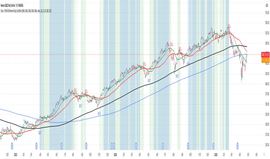
5ma + O’Neil & Minervini Buy ConditionIndicator Overview
5ma + O’Neil & Minervini Buy Condition is an original TradingView indicator that extends beyond a simple collection of standard moving averages by offering:
- Five Fully Independent Lines : Each of MA1–MA5 can be configured as SMA, EMA, WMA, or VWMA with its own period and data source. This level of customization unlocks unique combinations no existing script provides.
- Synergy of Multiple Timeframes : Default settings (10, 21, 50, 200, 325) reflect ultra‑short, short, medium, long, and volume‑weighted long‑term perspectives. The layered structure functions as a multi‑filter, sharpening entry signals and trend confirmation beyond any single MA.
- Integrated Buy Conditions : Built‑in O’Neil and Minervini buy filters use fixed SMA‑based rules (50 & 200 SMA rising within 15% of 52‑week high; 10 > 21 > 50 SMA rising within high/low thresholds), plus a combined condition highlighting when both methods align.
- Clean Visualization & Style Controls : Background coloring for each buy condition appears only in the Style tab under clearly named parameters (O’Neil Buy Condition, Minervini Buy Condition, Both Conditions). MA lines support transparent default colors and customizable line width for optimal readability without clutter.
Calculation & Logic
SMA: (P₁ + P₂ + … + Pₙ) ÷ N
EMA: α = 2 ÷ (N + 1)
EMA_today = (Price_today – EMA_yesterday) × α + EMA_yesterday
WMA: (P₁×N + P₂×(N–1) + … + Pₙ×1) ÷
VWMA: Σ(Pᵢ×Vᵢ) ÷ Σ(Vᵢ) for i = 1…N
```
Buy Condition Logic
- O’Neil: Price > 50 SMA & 200 SMA (both rising) **and** within 15% of the 52‑week high.
- Minervini : 10 SMA > 21 SMA > 50 SMA (both short‑term SMAs rising) **and** within 25% of the 52‑week high **and** at least 25% above the 52‑week low.
- Combined : Both O’Neil and Minervini conditions true.
Usage Examples
1. Short‑Mid Cross : Observe MA1/MA2 crossover while MA3/MA4 confirm trend strength.
2. Volume‑Weighted Long‑Term : Use VWMA as MA5 to filter institutional‑strength pullbacks.
3. Multi‑Filter Entry : Look for purple background (Both Conditions) on daily chart as high‑confidence entry.
Why It’s Unique
- Not a Mash‑Up : Though built on standard MA formulas, the customizable layering and built‑in buy filters create a novel multi‑dimensional analysis tool.
- Trader‑Friendly : Detailed comments in the code explain parameter choices, calculation methods, and practical entry scenarios so that even Pine novices can understand the underlying mechanics.
- Publication‑Ready : Description and code demonstrate originality, add clear value, and comply with house‑rule requirements by explaining why and how components interact, not just listing features.
- Combined Custom MA & Buy Conditions : By integrating customizable moving averages with built-in buy filters, users can easily recognize O’Neil and Minervini recommended setups.
Cerca negli script per "200亿美元是多少人民币"
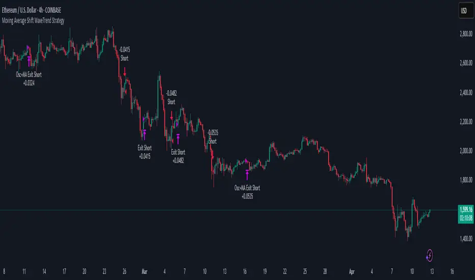
Moving Average Shift WaveTrend StrategyMoving Average Shift WaveTrend Strategy
🧭 Overview
The Moving Average Shift WaveTrend Strategy is a trend-following and momentum-based trading system designed to be overlayed on TradingView charts. It executes trades based on the confluence of multiple technical conditions—volatility, session timing, trend direction, and oscillator momentum—to deliver logical and systematic trade entries and exits.
🎯 Strategy Objectives
Enter trades aligned with the prevailing long-term trend
Exit trades on confirmed momentum reversals
Avoid false signals using session timing and volatility filters
Apply structured risk management with automatic TP, SL, and trailing stops
⚙️ Key Features
Selectable MA types: SMA, EMA, SMMA (RMA), WMA, VWMA
Dual-filter logic using a custom oscillator and moving averages
Session and volatility filters to eliminate low-quality setups
Trailing stop, configurable Take Profit / Stop Loss logic
“In-wave flag” prevents overtrading within the same trend wave
Visual clarity with color-shifting candles and entry/exit markers
📈 Trading Rules
✅ Long Entry Conditions:
Price is above the selected MA
Oscillator is positive and rising
200-period EMA indicates an uptrend
ATR exceeds its median value (sufficient volatility)
Entry occurs between 09:00–17:00 (exchange time)
Not currently in an active wave
🔻 Short Entry Conditions:
Price is below the selected MA
Oscillator is negative and falling
200-period EMA indicates a downtrend
All other long-entry conditions are inverted
❌ Exit Conditions:
Take Profit or Stop Loss is hit
Opposing signals from oscillator and MA
Trailing stop is triggered
🛡️ Risk Management Parameters
Pair: ETH/USD
Timeframe: 4H
Starting Capital: $3,000
Commission: 0.02%
Slippage: 2 pips
Risk per Trade: 2% of account equity (adjustable)
Total Trades: 224
Backtest Period: May 24, 2016 — April 7, 2025
Note: Risk parameters are fully customizable to suit your trading style and broker conditions.
🔧 Trading Parameters & Filters
Time Filter: Trades allowed only between 09:00–17:00 (exchange time)
Volatility Filter: ATR must be above its median value
Trend Filter: Long-term 200-period EMA
📊 Technical Settings
Moving Average
Type: SMA
Length: 40
Source: hl2
Oscillator
Length: 15
Threshold: 0.5
Risk Management
Take Profit: 1.5%
Stop Loss: 1.0%
Trailing Stop: 1.0%
👁️ Visual Support
MA and oscillator color changes indicate directional bias
Clear chart markers show entry and exit points
Trailing stops and risk controls are transparently managed
🚀 Strategy Improvements & Uniqueness
In-wave flag avoids repeated entries within the same trend phase
Filtering based on time, volatility, and trend ensures higher-quality trades
Dynamic high/low tracking allows precise trailing stop placement
Fully rule-based execution reduces emotional decision-making
💡 Inspirations & Attribution
This strategy is inspired by the excellent concept from:
ChartPrime – “Moving Average Shift”
It expands on the original idea with advanced trade filters and trailing logic.
Source reference:
📌 Summary
The Moving Average Shift WaveTrend Strategy offers a rule-based, reliable approach to trend trading. By combining trend and momentum filters with robust risk controls, it provides a consistent framework suitable for various market conditions and trading styles.
⚠️ Disclaimer
This script is for educational purposes only. Trading involves risk. Always use proper backtesting and risk evaluation before applying in live markets.
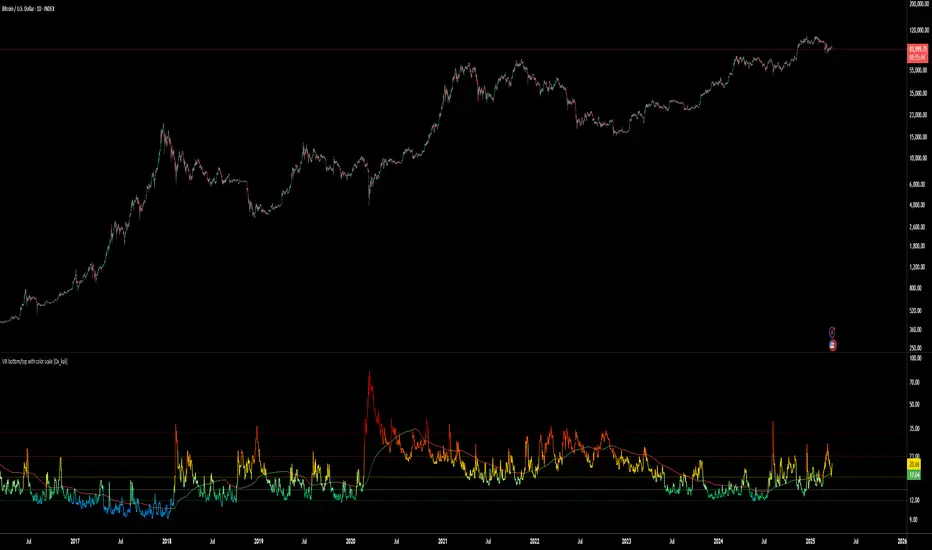
VIX bottom/top with color scale [Ox_kali]📊 Introduction
━━━━━━━━━━━━━━━━━━━━━━━━━━━━━━━━━━━━━━━━━━━
The “VIX Bottom/Top with Color Scale” script is designed to provide an intuitive, color-coded visualization of the VIX (Volatility Index), helping traders interpret market sentiment and volatility extremes in real time.
It segments the VIX into clear threshold zones, each associated with a specific market condition—ranging from fear to calm—using a dynamic color-coded system.
This script offers significant value for the following reasons:
Intuitive Risk Interpretation: Color-coded zones make it easy to interpret market sentiment at a glance.
Dynamic Trend Detection: A 200-period SMA of the VIX is plotted and dynamically colored based on trend direction.
Customization and Flexibility: All colors are editable in the parameters panel, grouped under “## Color parameters ##”.
Visual Clarity: Key thresholds are marked with horizontal lines for quick reference.
Practical Trading Tool: Helps identify high-risk and low-risk environments based on volatility levels.
🔍 Key Indicators
━━━━━━━━━━━━━━━━━━━━━━━━━━━━━━━━━━━━━━━━━━━
VIX (CBOE Volatility Index) : Measures market volatility and investor fear.
SMA 200 : Long-term trendline of the VIX, with color-coded direction (green = uptrend, red = downtrend).
Color-coded VIX Levels:
🔴 33+ → Something bad just happened
🟠 23–33 → Something bad is happening
🟡 17–23 → Something bad might happen
🟢 14–17 → Nothing bad is happening
✅ 12–14 → Nothing bad will ever happen
🔵 <12 → Something bad is going to happen
🧠 Originality and Purpose
━━━━━━━━━━━━━━━━━━━━━━━━━━━━━━━━━━━━━━━━━━━
Unlike traditional VIX indicators that only plot a line, this script enhances interpretation through visual segmentation and dynamic trend tracking.
It serves as a risk-awareness tool that transforms the VIX into a simple, emotional market map.
This is the first version of the script, and future updates may include alerts, background fills, and more advanced features.
⚙️ How It Works
━━━━━━━━━━━━━━━━━━━━━━━━━━━━━━━━━━━━━━━━━━━
The script maps the current VIX value to a range and applies the corresponding color.
It calculates a SMA 200 and colors it green or red depending on its slope.
It displays horizontal dotted lines at key thresholds (12, 14, 17, 23, 33).
All colors are configurable via input parameters under the group: "## Color parameters ##".
🧭 Indicator Visualization and Interpretation
━━━━━━━━━━━━━━━━━━━━━━━━━━━━━━━━━━━━━━━━━━━
The VIX line changes color based on market condition zones.
The SMA line shows long-term direction with dynamic color.
Horizontal threshold lines visually mark the transitions between volatility zones.
Ideal for quickly identifying periods of fear, caution, or stability.
🛠️ Script Parameters
━━━━━━━━━━━━━━━━━━━━━━━━━━━━━━━━━━━━━━━━━━━
Grouped under “## Color parameters ##”, the following elements are customizable:
🎨 VIX Zone Colors:
33+ → Red
23–33 → Orange
17–23 → Yellow
14–17 → Light Green
12–14 → Dark Green
<12 → Blue
📈 SMA Colors:
Uptrend → Green
Downtrend → Red
These settings allow users to match the script’s visuals to their preferred chart style or theme.
✅ Conclusion
━━━━━━━━━━━━━━━━━━━━━━━━━━━━━━━━━━━━━━━━━━━
The “VIX Bottom/Top with Color Scale” is a clean, powerful script designed to simplify how traders view volatility.
By combining long-term trend data with real-time color-coded sentiment analysis, this script becomes a go-to reference for managing risk, timing trades, or simply staying in tune with market mood.
🧪 Notes
━━━━━━━━━━━━━━━━━━━━━━━━━━━━━━━━━━━━━━━━━━━
This is version 1 of the script. More features such as alert conditions, background fill, and dashboard elements may be added soon. Feedback is welcome!
💡 Color code concept inspired by the original VIX interpretation chart by @nsquaredvalue on Twitter. Big thanks for the visual clarity! 💡
⚠️ Disclaimer
━━━━━━━━━━━━━━━━━━━━━━━━━━━━━━━━━━━━━━━━━━━
This script is a visual tool designed to assist in market analysis. It does not guarantee future performance and should be used in conjunction with proper risk management. Past performance is not indicative of future results.
Advanced Swing High/Low Trend Lines with MA Filter# Advanced Swing High/Low Trend Lines Indicator
## Overview
This advanced indicator identifies and draws trend lines based on swing highs and lows across three different timeframes (large, middle, and small trends). It's designed to help traders visualize market structure and potential support/resistance levels at multiple scales simultaneously.
## Key Features
- *Multi-Timeframe Analysis*: Simultaneously tracks trends at large (200-bar), middle (100-bar), and small (50-bar) scales
- *Customizable Visualization*: Different colors, widths, and styles for each trend level
- *Trend Confirmation System*: Requires minimum consecutive pivot points to validate trends
- *Trend Filter Option*: Can align trends with 200 EMA direction for consistency
## Recommended Settings
### For Long-Term Investors:
- Large Swing Length: 200-300
- Middle Swing Length: 100-150
- Small Swing Length: 50-75
- Enable Trend Filter: Yes
- Confirmation Points: 4-5
### For Swing Traders:
- Large Swing Length: 100
- Middle Swing Length: 50
- Small Swing Length: 20-30
- Enable Trend Filter: Optional
- Confirmation Points: 3
### For Day Traders:
- Large Swing Length: 50
- Middle Swing Length: 20
- Small Swing Length: 5-10
- Enable Trend Filter: No
- Confirmation Points: 2-3
## How to Use
### Identification:
1. *Large Trend Lines* (Red/Green): Show major market structure
2. *Middle Trend Lines* (Purple/Aqua): Intermediate levels
3. *Small Trend Lines* (Orange/Blue): Short-term price action
### Trading Applications:
- *Breakout Trading*: Watch for price breaking through multiple trend lines
- *Bounce Trading*: Look for reactions at confluence of trend lines
- *Trend Confirmation*: Aligned trends across timeframes suggest stronger moves
### Best Markets:
- Works well in trending markets (forex, indices)
- Effective in higher timeframes (1H+)
- Can be used in ranging markets to identify boundaries
## Customization Tips
1. For cleaner charts, reduce line widths in congested markets
2. Use dotted styles for smaller trends to reduce visual clutter
3. Adjust confirmation points based on market volatility (higher for noisy markets)
## Limitations
- May repaint on current swing points
- Works best in trending conditions
- Requires sufficient historical data for longer swing lengths
This indicator provides a comprehensive view of market structure across multiple timeframes, helping traders make more informed decisions by visualizing the hierarchy of support and resistance levels.

Multi-Indicator Trading DashboardMulti-Indicator Trading Dashboard: Comprehensive Analysis and Actionable Signals
This Pine Script indicator, "Multi-Indicator Trading Dashboard," provides a comprehensive overview of key market indicators and generates actionable trading signals, all presented in a clear, easy-to-read table format on your TradingView chart.
Key Features:
Real-time Indicator Analysis: The dashboard displays real-time values and signals for:
RSI (Relative Strength Index): Tracks overbought and oversold conditions.
MACD (Moving Average Convergence Divergence): Identifies trend changes and momentum.
ADX (Average Directional Index): Measures trend strength.
Volatility (ATR-based): Estimates volatility as a percentage, acting as a VIX proxy for single-symbol charts.
Trend Determination: Analyzes 20, 50, and 200-period EMAs to provide a clear trend assessment (Strong Bullish, Cautious Bullish, Cautious Bearish, Strong Bearish).
Combined Trading Signals: Integrates signals from RSI, MACD, ADX, and trend analysis to generate a combined "Buy," "Sell," or "Neutral" action signal.
User-Friendly Table Display: Presents all information in a neatly organized table, positioned at the top-right of your chart.
Visual Chart Overlays: Plots 20, 50, and 200-period EMAs directly on the chart for visual trend confirmation.
Background Color Alerts: Colors the chart's background based on the "Buy" or "Sell" action signal for quick visual cues.
Customizable Inputs: Allows you to adjust key parameters like RSI lengths, MACD settings, ADX thresholds, and EMA periods.
How It Works:
Indicator Calculations: The script calculates RSI, MACD, ADX, and a volatility proxy (ATR) using standard Pine Script functions.
Trend Analysis: It compares 20, 50, and 200-period EMAs to determine the overall trend direction.
Individual Signal Generation: It generates individual "Buy," "Sell," or "Neutral" signals based on RSI, MACD, and ADX values.
Combined Signal Logic: It combines the individual signals and trend analysis, assigning a "Buy" or "Sell" action only when at least two indicators align.
Table Display: It creates a table and populates it with the calculated values, signals, and trend information.
Chart Overlays: It plots the EMAs on the chart and colors the background based on the combined action signal.
Use Cases:
Quick Market Overview: Get a snapshot of key market indicators and trend direction at a glance.
Confirmation Tool: Use the combined signals to confirm your existing trading strategies.
Educational Purpose: Learn how different indicators interact and influence trading decisions.
Automated Alerting: Set up alerts based on the "Buy" or "Sell" action signals.
Customization:
Adjust the input parameters to fine-tune the indicator's sensitivity to your trading style and the specific market you're analyzing.
Disclaimer:
This indicator is for informational and educational purposes only and should not be considered financial advice. Always conduct thorough research and consult with 1 a qualified professional before making any 2 trading decisions.

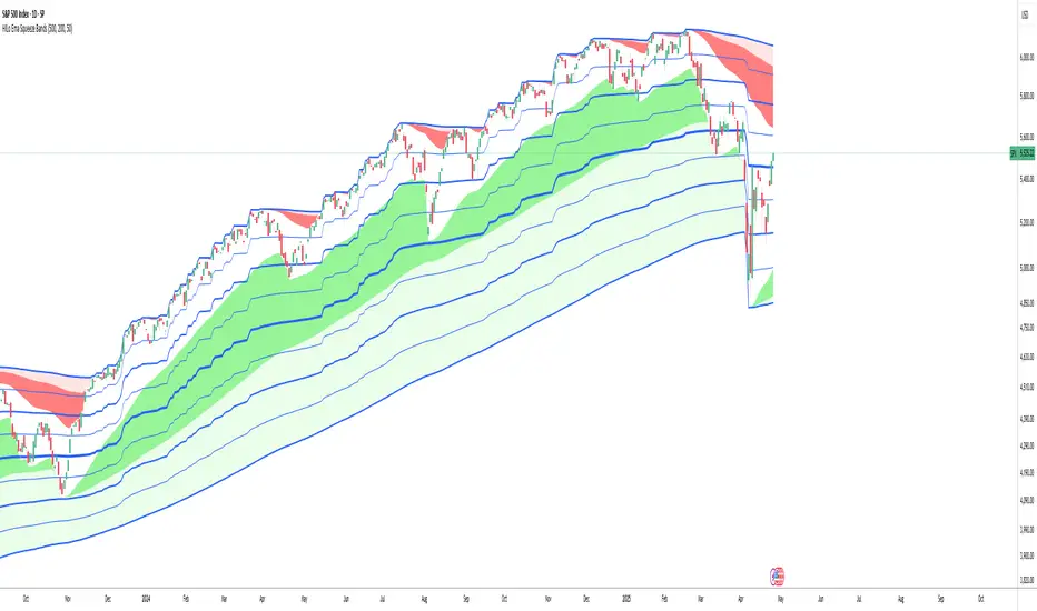
HILo Ema Squeeze BandsThis indicator combines uses ema to identify price squeeze before a big move.
The ema gets initialised at new high low. It used 3 ema's lengths. For result use x, 2x ,4x ie 50, 100, 200 or 100,200,400 and so on . On more volatile asset use a higher settings like 100,200,400. The inner band is divided into 4 zones, which can give support resistance. As you use it you will become aware of subtle information that it can give at times. Like you may be able to find steps at which prices move, when the market is trending
Just like in Bollinger bands, in a trending market the price stays within sd=1 and sd=2 so does in the inner band the price will remain in band1 and band2. But Bollinger band cannot print steps this indicator shows steps
Adaptive Regression Channel [MissouriTim]The Adaptive Regression Channel (ARC) is a technical indicator designed to empower traders with a clear, adaptable, and precise view of market trends and price boundaries. By blending advanced statistical techniques with real-time market data, ARC delivers a comprehensive tool that dynamically adjusts to price action, volatility, volume, and momentum. Whether you’re navigating the fast-paced world of cryptocurrencies, the steady trends of stocks, or the intricate movements of FOREX pairs, ARC provides a robust framework for identifying opportunities and managing risk.
Core Components
1. Color-Coded Regression Line
ARC’s centerpiece is a linear regression line derived from a Weighted Moving Average (WMA) of closing prices. This line adapts its calculation period based on market volatility (via ATR) and is capped between a minimum of 20 bars and a maximum of 1.5 times the user-defined base length (default 100). Visually, it shifts colors to reflect trend direction: green for an upward slope (bullish) and red for a downward slope (bearish), offering an instant snapshot of market sentiment.
2. Dynamic Residual Channels
Surrounding the regression line are upper (red) and lower (green) channels, calculated using the standard deviation of residuals—the difference between actual closing prices and the regression line. This approach ensures the channels precisely track how closely prices follow the trend, rather than relying solely on overall price volatility. The channel width is dynamically adjusted by a multiplier that factors in:
Volatility: Measured through the Average True Range (ATR), widening channels during turbulent markets.
Trend Strength: Based on the regression slope, expanding channels in strong trends and contracting them in consolidation phases.
3. Volume-Weighted Moving Average (VWMA)
Plotted in orange, the VWMA overlays a volume-weighted price trend, emphasizing movements backed by significant trading activity. This complements the regression line, providing additional confirmation of trend validity and potential breakout strength.
4. Scaled RSI Overlay
ARC features a Relative Strength Index (RSI) overlay, plotted in purple and scaled to hover closely around the regression line. This compact display reflects momentum shifts within the trend’s context, keeping RSI visible on the price chart without excessive swings. User-defined overbought (default 70) and oversold (default 30) levels offer reference points for momentum analysis."
Technical Highlights
ARC leverages a volatility-adjusted lookback period, residual-based channel construction, and multi-indicator integration to achieve high accuracy. Its parameters—such as base length, channel width, ATR period, and RSI length—are fully customizable, allowing traders to tailor it to their specific needs.
Why Choose ARC?
ARC stands out for its adaptability and precision. The residual-based channels offer tighter, more relevant support and resistance levels compared to standard volatility measures, while the dynamic adjustments ensure it performs well in both trending and ranging markets. The inclusion of VWMA and scaled RSI adds depth, merging trend, volume, and momentum into a single, cohesive overlay. For traders seeking a versatile, all-in-one indicator, ARC delivers actionable insights with minimal noise.
Best Ways to Use the Adaptive Regression Channel (ARC)
The Adaptive Regression Channel (ARC) is a flexible tool that supports a variety of trading strategies, from trend-following to breakout detection. Below are the most effective ways to use ARC, along with practical tips for maximizing its potential. Adjustments to its settings may be necessary depending on the timeframe (e.g., intraday vs. daily) and the asset being traded (e.g., stocks, FOREX, cryptocurrencies), as each market exhibits unique volatility and behavior.
1. Trend Following
• How to Use: Rely on the regression line’s color to guide your trades. A green line (upward slope) signals a bullish trend—consider entering or holding long positions. A red line (downward slope) indicates a bearish trend—look to short or exit longs.
• Best Practice: Confirm the trend with the VWMA (orange line). Price above the VWMA in a green uptrend strengthens the bullish case; price below in a red downtrend reinforces bearish momentum.
• Adjustment: For short timeframes like 15-minute crypto charts, lower the Base Regression Length (e.g., to 50) for quicker trend detection. For weekly stock charts, increase it (e.g., to 200) to capture broader movements.
2. Channel-Based Trades
• How to Use: Use the upper channel (red) as resistance and the lower channel (green) as support. Buy when the price bounces off the lower channel in an uptrend, and sell or short when it rejects the upper channel in a downtrend.
• Best Practice: Check the scaled RSI (purple line) for momentum cues. A low RSI (e.g., near 30) at the lower channel suggests a stronger buy signal; a high RSI (e.g., near 70) at the upper channel supports a sell.
• Adjustment: In volatile crypto markets, widen the Base Channel Width Coefficient (e.g., to 2.5) to reduce false signals. For stable FOREX pairs (e.g., EUR/USD), a narrower width (e.g., 1.5) may work better.
3. Breakout Detection
• How to Use: Watch for price breaking above the upper channel (bullish breakout) or below the lower channel (bearish breakout). These moves often signal strong momentum shifts.
• Best Practice: Validate breakouts with VWMA position—price above VWMA for bullish breaks, below for bearish—and ensure the regression line’s slope aligns (green for up, red for down).
• Adjustment: For fast-moving assets like crypto on 1-hour charts, shorten ATR Length (e.g., to 7) to make channels more reactive. For stocks on daily charts, keep it at 14 or higher for reliability.
4. Momentum Analysis
• How to Use: The scaled RSI overlay shows momentum relative to the regression line. Rising RSI in a green uptrend confirms bullish strength; falling RSI in a red downtrend supports bearish pressure.
• Best Practice: Look for RSI divergences—e.g., price hitting new highs at the upper channel while RSI flattens or drops could signal an impending reversal.
• Adjustment: Reduce RSI Length (e.g., to 7) for intraday trading in FOREX or crypto to catch short-term momentum shifts. Increase it (e.g., to 21) for longer-term stock trades.
5. Range Trading
• How to Use: When the regression line’s slope is near zero (flat) and channels are tight, ARC indicates a ranging market. Buy near the lower channel and sell near the upper channel, targeting the regression line as the mean price.
• Best Practice: Ensure VWMA hovers close to the regression line to confirm the range-bound state.
• Adjustment: For low-volatility stocks on daily charts, use a moderate Base Regression Length (e.g., 100) and tight Base Channel Width (e.g., 1.5). For choppy crypto markets, test shorter settings.
Optimization Strategies
• Timeframe Customization: Adjust ARC’s parameters to match your trading horizon. Short timeframes (e.g., 1-minute to 1-hour) benefit from lower Base Regression Length (20–50) and ATR Length (7–10) for agility, while longer timeframes (e.g., daily, weekly) favor higher values (100–200 and 14–21) for stability.
• Asset-Specific Tuning:
○ Stocks: Use longer lengths (e.g., 100–200) and moderate widths (e.g., 1.8) for stable equities; tweak ATR Length based on sector volatility (shorter for tech, longer for utilities).
○ FOREX: Set Base Regression Length to 50–100 and Base Channel Width to 1.5–2.0 for smoother trends; adjust RSI Length (e.g., 10–14) based on pair volatility.
○ Crypto: Opt for shorter lengths (e.g., 20–50) and wider widths (e.g., 2.0–3.0) to handle rapid price swings; use a shorter ATR Length (e.g., 7) for quick adaptation.
• Backtesting: Test ARC on historical data for your asset and timeframe to optimize settings. Evaluate how often price respects channels and whether breakouts yield profitable trades.
• Enhancements: Pair ARC with volume surges, key support/resistance levels, or candlestick patterns (e.g., doji at channel edges) for higher-probability setups.
Practical Considerations
ARC’s adaptability makes it suitable for diverse markets, but its performance hinges on proper calibration. Cryptocurrencies, with their high volatility, may require shorter, wider settings to capture rapid moves, while stocks on longer timeframes benefit from broader, smoother configurations. FOREX pairs often fall in between, depending on their inherent volatility. Experiment with the adjustable parameters to align ARC with your trading style and market conditions, ensuring it delivers the precision and reliability you need.

MACD with TrendIndicator Name: MACD with Trend & Multi-Timeframe Dashboard
Why Use This Indicator?
Two MACDs for Double Confirmation:
It integrates both a standard MACD (fast/slow lengths of your choice) and a Trend MACD (longer lengths). The standard MACD identifies short-term momentum shifts, while the Trend MACD helps confirm the higher-level market trend.
Multi-Timeframe 50/200 SMA Overview:
A built-in dashboard quickly shows whether the 50-period moving average is above or below the 200-period moving average across multiple timeframes (Monthly, Weekly, Daily, etc.). At a glance, you can see if higher timeframes agree with your immediate trading setup.
Clear Buy/Sell Signals:
The script plots buy arrows when the MACD histogram crosses from negative to positive, plus an additional label for the Trend MACD crossing. The same goes for sell signals if momentum flips from positive to negative. This clarity can reduce guesswork.
Customizable & Intuitive:
Easily adjust moving average types (SMA or EMA), lengths, and source inputs to suit different asset classes or personal preferences. Visual color coding helps you quickly interpret bullish vs. bearish conditions.
Recommended Trading Approach
Identify Overall Trend
Check the Trend MACD histogram and the multi-timeframe dashboard (50/200 SMAs). If you see bullish alignment on higher timeframes (e.g., Daily, Weekly) and the Trend MACD is above zero, you know the market environment is supportive for long trades.
Pinpoint Entry Using Standard MACD
Wait for the standard MACD histogram to cross above zero or for a labeled “Buy Signal.” This indicates short-term momentum turning bullish in sync with the broader trend. If the market is already trending up (confirmed by the dashboard), the probability of a successful long entry often improves.
Set a Stop-Loss & Take-Profit
While not included in the code, adding an ATR- or price-based stop-loss can protect against sudden reversals. A simple approach is risking 1–2% per trade and aiming for a 1.5–2× reward relative to that risk.
Monitor Sell Signals
If the short-term MACD crosses below zero—triggering a “Sell Signal”—and the Trend MACD also turns down (or the dashboard flips bearish), consider exiting the position or tightening stops. This alignment of short- and long-term indicators often signals a shift in momentum that could threaten your open profits.
Summary
The MACD with Trend & Multi-Timeframe Dashboard is a versatile, all-in-one toolkit. It combines the immediacy of short-term MACD signals, the validation of a longer-term trend oscillator, and the broader insight of multi-timeframe moving averages. Whether you are a swing trader looking for alignment across bigger trends or a shorter-term trader wanting clear momentum triggers, this indicator helps streamline decision-making and reduce noise.
Disclaimer: As with all technical analysis tools, there is no guarantee of success. Always combine indicator signals with sound risk management and a thorough understanding of market conditions

Trend Detection
#### *Description:*
This *Trend Detection* indicator is designed to help traders identify and confirm trends in the market using a combination of moving averages, volume analysis, and MACD filters. It provides clear visual signals for uptrends and downtrends, along with customizable settings to adapt to different trading styles and timeframes. The indicator is suitable for both beginners and advanced traders who want to improve their trend-following strategies.
---
#### *Key Features:*
1. *Trend Detection:*
- Uses *Moving Averages (MA)* to determine the overall trend direction.
- Supports multiple MA types: *SMA (Simple), **EMA (Exponential), **WMA (Weighted), and **HMA (Hull)*.
2. *Advanced Filters:*
- *MACD Filter:* Confirms trends using MACD crossovers.
- *Volume Filter:* Ensures trends are supported by above-average volume.
- *Multi-Timeframe Filter:* Validates trends using a higher timeframe (e.g., Daily or Weekly).
3. *Visual Signals:*
- Plots a *trend line* on the chart to indicate the current trend direction.
- Fills the background with *green* for uptrends and *red* for downtrends.
4. *Customizable Settings:*
- Adjust the *MA lengths, **MACD parameters, and **confirmation thresholds* to suit your trading strategy.
- Control the transparency of the background fill for better chart readability.
5. *Alerts:*
- Generates *buy/sell signals* when a trend is confirmed.
- Alerts can be set to trigger at the close of a candle for precise entry/exit points.
---
#### *How to Use:*
1. *Adding the Indicator:*
- Copy and paste the Pine Script code into the TradingView Pine Script editor.
- Add the indicator to your chart.
2. *Configuring the Settings:*
- *Trend Settings:*
- Choose the *MA type* (e.g., EMA for faster response, HMA for smoother trends).
- Set the *Trend MA Period* (e.g., 200 for long-term trends) and *Filter MA Period* (e.g., 100 for medium-term trends).
- *Advanced Filters:*
- Enable/disable the *MACD Filter* and adjust its parameters (Fast, Slow, Signal).
- Enable/disable the *Volume Filter* to ensure trends are supported by volume.
- *Multi-Timeframe Filter:*
- Enable this filter to validate trends using a higher timeframe (e.g., Daily or Weekly).
3. *Interpreting the Signals:*
- *Uptrend:* The trend line turns *green*, and the background is filled with a transparent green color.
- *Downtrend:* The trend line turns *red*, and the background is filled with a transparent red color.
- *Alerts:* Buy/sell signals are generated when the trend is confirmed.
4. *Using Alerts:*
- Set up alerts for *Buy Signal* (bullish reversal) and *Sell Signal* (bearish reversal).
- Alerts can be configured to trigger at the close of a candle for precise execution.
---
#### *Settings and Their Effects:*
1. *MA Type:*
- *SMA:* Smooth but lagging. Best for long-term trends.
- *EMA:* Faster response to price changes. Suitable for medium-term trends.
- *WMA:* Gives more weight to recent prices. Useful for short-term trends.
- *HMA:* Combines speed and smoothness. Ideal for all timeframes.
2. *Trend MA Period:*
- A longer period (e.g., 200) identifies long-term trends but may lag.
- A shorter period (e.g., 50) reacts faster but may produce false signals.
3. *Filter MA Period:*
- Acts as a secondary filter to confirm the trend.
- A shorter period (e.g., 50) provides tighter confirmation but may increase noise.
4. *MACD Filter:*
- Ensures trends are confirmed by MACD crossovers.
- Adjust the *Fast, **Slow, and **Signal* lengths to match your trading style.
5. *Volume Filter:*
- Ensures trends are supported by above-average volume.
- Reduces false signals during low-volume periods.
6. *Multi-Timeframe Filter:*
- Validates trends using a higher timeframe (e.g., Daily or Weekly).
- Increases reliability but may delay signals.
7. *Confirmation Value:*
- Sets the minimum percentage deviation from the trend MA required to confirm a trend.
- A higher value (e.g., 2.0%) reduces false signals but may delay trend detection.
8. *Confirmation Bars:*
- Sets the number of bars required to confirm a trend.
- A higher value (e.g., 5 bars) ensures sustained trends but may delay signals.
---
#### *Who Should Use This Indicator?*
1. *Trend Followers:*
- Traders who focus on identifying and riding long-term trends.
- Suitable for *swing traders* and *position traders*.
2. *Day Traders:*
- Can use shorter MA periods and faster filters (e.g., EMA, HMA) for intraday trends.
3. *Volume-Based Traders:*
- Traders who rely on volume confirmation to validate trends.
4. *Multi-Timeframe Traders:*
- Traders who use higher timeframes to confirm trends on lower timeframes.
5. *Beginners:*
- Easy-to-understand visual signals and alerts make it beginner-friendly.
6. *Advanced Traders:*
- Customizable settings allow for fine-tuning to match specific strategies.
---
#### *Example Use Cases:*
1. *Long-Term Investing:*
- Use a *200-period SMA* with a *Daily* higher timeframe filter to identify long-term trends.
- Enable the *Volume Filter* to ensure trends are supported by strong volume.
2. *Swing Trading:*
- Use a *50-period EMA* with a *4-hour* higher timeframe filter for medium-term trends.
- Enable the *MACD Filter* to confirm trend reversals.
3. *Day Trading:*
- Use a *20-period HMA* with a *1-hour* higher timeframe filter for short-term trends.
- Disable the *Volume Filter* for faster signals.
---
#### *Conclusion:*
The *Trend Detection* indicator is a versatile tool for traders of all levels. Its customizable settings and advanced filters make it suitable for various trading styles and timeframes. By combining moving averages, volume analysis, and MACD filters, it provides reliable trend signals with minimal lag. Whether you're a beginner or an advanced trader, this indicator can help you make better trading decisions by identifying and confirming trends in the market.
---
#### *Publishing on TradingView:*
- *Title:* Trend Detection with Advanced Filters
- *Description:* A powerful trend detection tool using moving averages, volume analysis, and MACD filters. Suitable for all trading styles and timeframes.
- *Tags:* Trend, Moving Averages, MACD, Volume, Multi-Timeframe
- *Category:* Trend-Following
- *Access:* Public or Private (depending on your preference).
---
Let me know if you need further assistance or additional features!
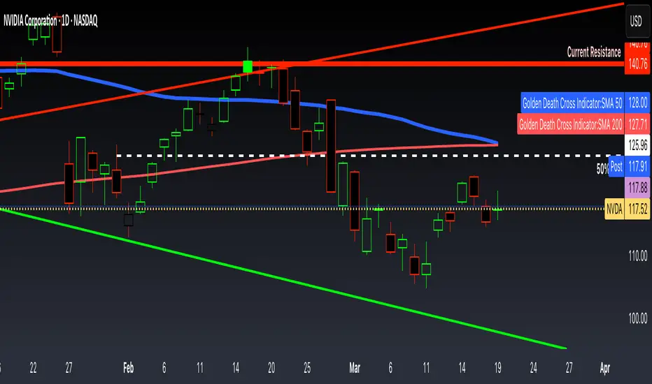
Golden Death Cross IndicatorThis indicator uses moving average to detect both a Golden Cross and Death Cross on any timeframe but is recommended for use on the daily and 24 hour timeframes only.
We have also provided instructions on how to create alerts for these indicators below.
Happy Trading!
Moving Averages: We’ll use Simple Moving Averages (SMA). The 50-day SMA looks at the average price over the last 50 periods, and the 200-day SMA does the same for 200 periods.
Crossovers: We’ll check when the 50-day SMA crosses above (Golden Cross) or below the 200-day SMA (Death Cross).
Set Up Alerts
Now, let’s make sure you get notified when a cross happens:
Open the Alerts Menu
On the chart, click the bell icon (top right of the screen) to create an alert.
Configure the Golden Cross Alert
In the “Condition” dropdown, select “Cross Alerts” (the name of your script).
Below that, select “Golden Cross.”
Set “Once Per Bar Close” in the next dropdown (this ensures it only triggers after the period ends, avoiding false signals mid-bar).
Choose how you want to be notified (e.g., popup, email, or phone app—set this under “Notifications”).
Name the alert (e.g., “Golden Cross Alert”) and click “Create.”
Configure the Death Cross Alert
Click the bell icon again to create a second alert.
Condition: “Cross Alerts” > “Death Cross.”
Set “Once Per Bar Close” again.
Choose your notification method.
Name it (e.g., “Death Cross Alert”) and click “Create.”
TradZoo - EMA Crossover IndicatorDescription:
This EMA Crossover Trading Strategy is designed to provide precise Buy and Sell signals with confirmation, defined targets, and stop-loss levels, ensuring strong risk management. Additionally, a 30-candle gap rule is implemented to avoid frequent signals and enhance trade accuracy.
📌 Strategy Logic
✅ Exponential Moving Averages (EMAs):
Uses EMA 50 & EMA 200 for trend direction.
Buy signals occur when price action confirms EMA crossovers.
✅ Entry Confirmation:
Buy Signal: Occurs when either the current or previous candle touches the 200 EMA, and the next candle closes above the previous candle’s close.
Sell Signal: Occurs when either the current or previous candle touches the 200 EMA, and the next candle closes below the previous candle’s close.
✅ 30-Candle Gap Rule:
Prevents frequent entries by ensuring at least 30 candles pass before the next trade.
Improves signal quality and prevents excessive trading.
🎯 Target & Stop-Loss Calculation
✅ Buy Position:
Target: 2X the difference between the last candle’s close and the lowest low of the last 2 candles.
Stop Loss: The lowest low of the last 2 candles.
✅ Sell Position:
Target: 2X the difference between the last candle’s close and the highest high of the last 2 candles.
Stop Loss: The highest high of the last 2 candles.
📊 Visual Features
✅ Buy & Sell Signals:
Green Upward Arrow → Buy Signal
Red Downward Arrow → Sell Signal
✅ Target Levels:
Green Dotted Line: Buy Target
Red Dotted Line: Sell Target
✅ Stop Loss Levels:
Dark Red Solid Line: Stop Loss for Buy/Sell
💡 How to Use
🔹 Ideal for trend-following traders using EMAs.
🔹 Works best in volatile & trending markets (avoid sideways ranges).
🔹 Can be combined with RSI, MACD, or price action levels for added confluence.
🔹 Recommended timeframes: 1M, 5M, 15m, 1H, 4H, Daily (for best results).
🚀 Try this strategy and enhance your trading decisions with structured risk management!

MA Cross Multi Alert KrafturMA Cross Multi Alert Kraftur
Description
The "MA Cross Multi Alert Kraftur" indicator is a versatile tool designed to help traders identify potential buy and sell opportunities based on the crossings of multiple moving averages (MAs). Unlike traditional MA crossover indicators that focus on a single pair of averages, this script offers three distinct crossover levels (e.g., 21/50, 50/90, 50/200) for greater flexibility and precision. It overlays signals directly on the price chart and delivers real-time alerts when crossings occur, making it an excellent choice for traders seeking to pinpoint entry and exit points across various market conditions.
Key Features
Multi-Level Crossovers: Tracks crossings between configurable moving averages (e.g., 21 crossing 50, 50 crossing 90, 50 crossing 200) to detect varying trend strengths and reversals.
Visual Signals: Buy signals are displayed as upward triangles below the bars, and sell signals as downward triangles above the bars, each color-coded for quick recognition.
Real-Time Alerts: Triggers alerts once per bar when a crossover occurs, with a filter to avoid repetitive notifications during minor fluctuations.
Customizable: Adjustable MA lengths, timeframe, and signal colors allow tailoring to individual trading preferences and strategies.
Recommended Usage
This indicator shines as a scanning tool for identifying trade setups across multiple assets. Apply it to your watchlist of stocks, forex pairs, or cryptocurrencies, and set up alerts to catch crossover signals in real time. It performs exceptionally well in trending or consolidating markets and can be paired with additional tools (e.g., trendlines, RSI, or volume analysis) to validate signals and boost reliability. Ideal for multi-timeframe traders or those managing diverse portfolios.
How to Use
Add the indicator to your chart.
Adjust the MA lengths (e.g., 21, 50, 90, 200), timeframe, and signal colors to align with your trading approach.
Configure alerts for the indicator and apply them to your asset watchlist.
Watch for buy (upward triangles) and sell (downward triangles) signals on the chart, or rely on alert notifications for timely updates.
Perfect for day traders, swing traders, or anyone aiming to streamline signal detection and automate their workflow!
Put/Call RatioPut/Call Ratio Indicator
This indicator visualizes the Put/Call Ratio for various market symbols, helping traders assess market sentiment and potential reversals. It offers a dropdown menu to select from a range of Put/Call Ratios, including broad equities (CBOE), major indices (SPX, QQQ, IWM, VIX), and individual stocks (TSLA, GOOG, META, AMZN, MSFT, INTC).
The indicator plots the Put/Call Ratio with adjustable moving averages and standard deviation bands to highlight overbought or oversold conditions. A short-term moving average (default: 10 periods) is displayed with trend-based coloring, while longer-term moving averages (defaults: 30 and 200 periods) are calculated but hidden by default. Bands at 1, 1.5, and 2 standard deviations provide context for extreme readings.
Key Overbought/Oversold Signals:
Short-Term Extremes: The 10-day moving average moves beyond 1 standard deviation from the 200-day moving average, signaling potential overbought (above) or oversold (below) conditions. This will be highlighted by red or green background color.
Ratio Extremes: The Put/Call Ratio line itself crosses outside 2 standard deviations from the 200-day moving average, indicating stronger overbought or oversold zones.
Conditional coloring of the ratio line reflects its position relative to the bands, and background shading highlights when the short-term moving average crosses key levels.
Key Features:
Selectable Put/Call Ratio symbols.
Trend-colored moving averages.
Standard deviation bands for volatility analysis.
Dynamic line and background coloring for quick insights.
Usage:
Use this indicator to gauge market sentiment—high ratios may suggest bearish sentiment or oversold conditions, while low ratios may indicate bullish sentiment or overbought conditions. Combine with price action or other tools for confirmation.

[SHORT ONLY] ATR Sell the Rip Mean Reversion Strategy█ STRATEGY DESCRIPTION
The "ATR Sell the Rip Mean Reversion Strategy" is a contrarian system that targets overextended price moves on stocks and ETFs. It calculates an ATR‐based trigger level to identify shorting opportunities. When the current close exceeds this smoothed ATR trigger, and if the close is below a 200-period EMA (if enabled), the strategy initiates a short entry, aiming to profit from an anticipated corrective pullback.
█ HOW IS THE ATR SIGNAL BAND CALCULATED?
This strategy computes an ATR-based signal trigger as follows:
Calculate the ATR
The strategy computes the Average True Range (ATR) using a configurable period provided by the user:
atrValue = ta.atr(atrPeriod)
Determine the Threshold
Multiply the ATR by a predefined multiplier and add it to the current close:
atrThreshold = close + atrValue * atrMultInput
Smooth the Threshold
Apply a Simple Moving Average over a specified period to smooth out the threshold, reducing noise:
signalTrigger = ta.sma(atrThreshold, smoothPeriodInput)
█ SIGNAL GENERATION
1. SHORT ENTRY
A Short Signal is triggered when:
The current close is above the smoothed ATR signal trigger.
The trade occurs within the specified trading window (between Start Time and End Time).
If the EMA filter is enabled, the close must also be below the 200-period EMA.
2. EXIT CONDITION
An exit Signal is generated when the current close falls below the previous bar’s low (close < low ), indicating a potential bearish reversal and prompting the strategy to close its short position.
█ ADDITIONAL SETTINGS
ATR Period: The period used to calculate the ATR, allowing for adaptability to different volatility conditions (default is 20).
ATR Multiplier: The multiplier applied to the ATR to determine the raw threshold (default is 1.0).
Smoothing Period: The period over which the raw ATR threshold is smoothed using an SMA (default is 10).
Start Time and End Time: Defines the time window during which trades are allowed.
EMA Filter (Optional): When enabled, short entries are only executed if the current close is below the 200-period EMA, confirming a bearish trend.
█ PERFORMANCE OVERVIEW
This strategy is designed for use on the Daily timeframe, targeting stocks and ETFs by capitalizing on overextended price moves.
It utilizes a dynamic, ATR-based trigger to identify when prices have potentially peaked, setting the stage for a mean reversion short entry.
The optional EMA filter helps align trades with broader market trends, potentially reducing false signals.
Backtesting is recommended to fine-tune the ATR multiplier, smoothing period, and EMA settings to match the volatility and behavior of specific markets.

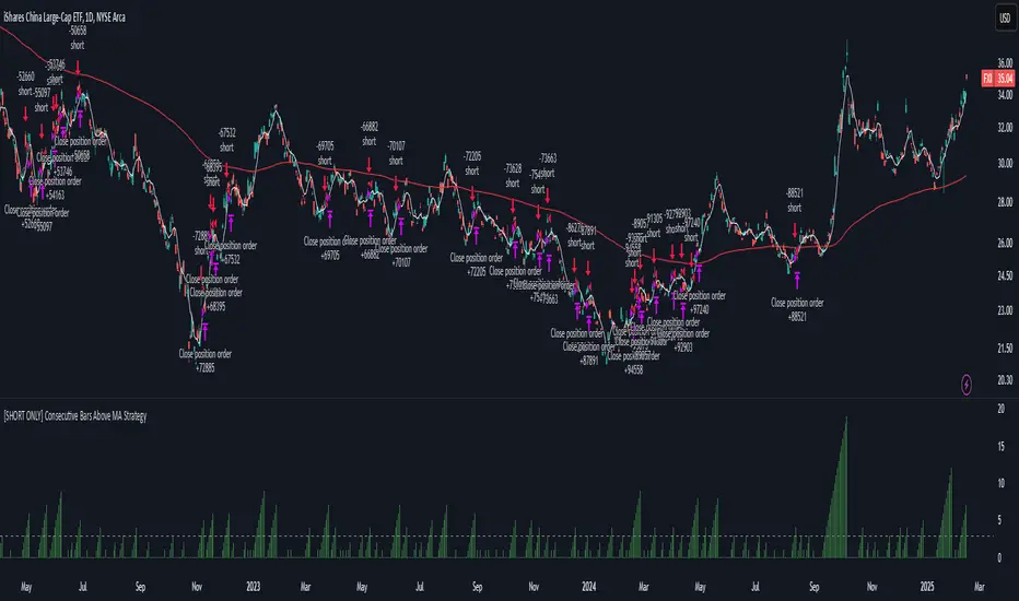
[SHORT ONLY] Consecutive Bars Above MA Strategy█ STRATEGY DESCRIPTION
The "Consecutive Bars Above MA Strategy" is a contrarian trading system aimed at exploiting overextended bullish moves in stocks and ETFs. It monitors the number of consecutive bars that close above a chosen short-term moving average (which can be either a Simple Moving Average or an Exponential Moving Average). Once the count reaches a preset threshold and the current bar’s close exceeds the previous bar’s high within a designated trading window, a short entry is initiated. An optional EMA filter further refines entries by requiring that the current close is below the 200-period EMA, helping to ensure that trades are taken in a bearish environment.
█ HOW ARE THE CONSECUTIVE BULLISH COUNTS CALCULATED?
The strategy utilizes a counter variable, `bullCount`, to track consecutive bullish bars based on their relation to the short-term moving average. Here’s how the count is determined:
Initialize the Counter
The counter is initialized at the start:
var int bullCount = na
Bullish Bar Detection
For each bar, if the close is above the selected moving average (either SMA or EMA, based on user input), the counter is incremented:
bullCount := close > signalMa ? (na(bullCount) ? 1 : bullCount + 1) : 0
Reset on Non-Bullish Condition
If the close does not exceed the moving average, the counter resets to zero, indicating a break in the consecutive bullish streak.
█ SIGNAL GENERATION
1. SHORT ENTRY
A short signal is generated when:
The number of consecutive bullish bars (i.e., bars closing above the short-term MA) meets or exceeds the defined threshold (default: 3).
The current bar’s close is higher than the previous bar’s high.
The signal occurs within the specified trading window (between Start Time and End Time).
Additionally, if the EMA filter is enabled, the entry is only executed when the current close is below the 200-period EMA.
2. EXIT CONDITION
An exit signal is triggered when the current close falls below the previous bar’s low, prompting the strategy to close the short position.
█ ADDITIONAL SETTINGS
Threshold: The number of consecutive bullish bars required to trigger a short entry (default is 3).
Trading Window: The Start Time and End Time inputs define when the strategy is active.
Moving Average Settings: Choose between SMA and EMA, and set the MA length (default is 5), which is used to assess each bar’s bullish condition.
EMA Filter (Optional): When enabled, this filter requires that the current close is below the 200-period EMA, supporting entries in a downtrend.
█ PERFORMANCE OVERVIEW
This strategy is designed for stocks and ETFs and can be applied across various timeframes.
It seeks to capture mean reversion by shorting after a series of bullish bars suggests an overextended move.
The approach employs a contrarian short entry by waiting for a breakout (close > previous high) following consecutive bullish bars.
The adjustable moving average settings and optional EMA filter allow for further optimization based on market conditions.
Comprehensive backtesting is recommended to fine-tune the threshold, moving average parameters, and filter settings for optimal performance.
2xSPYTIPS Strategy by Fra public versionThis is a test strategy with S&P500, open source so everyone can suggest everything, I'm open to any advice.
Rules of the "2xSPYTIPS" Strategy :
This trading strategy is designed to operate on the S&P 500 index and the TIPS ETF. Here’s how it works:
1. Buy Conditions ("BUY"):
- The S&P 500 must be above its **200-day simple moving average (SMA 200)**.
- This condition is checked at the **end of each month**.
2. Position Management:
- If leverage is enabled (**2x leverage**), the purchase quantity is increased based on a configurable percentage.
3. Take Profit:
- A **Take Profit** is set at a fixed percentage above the entry price.
4. Visualization & Alerts:
- The **SMA 200** for both S&P 500 and TIPS is plotted on the chart.
- A **BUY signal** appears visually and an alert is triggered.
What This Strategy Does NOT Do
- It does not use a **Stop Loss** or **Trailing Stop**.
- It does not directly manage position exits except through Take Profit.

Iron Bot Statistical Trend Filter📌 Iron Bot Statistical Trend Filter
📌 Overview
Iron Bot Statistical Trend Filter is an advanced trend filtering strategy that combines statistical methods with technical analysis.
By leveraging Z-score and Fibonacci levels, this strategy quantitatively analyzes market trends to provide high-precision entry signals.
Additionally, it includes an optional EMA filter to enhance trend reliability.
Risk management is reinforced with Stop Loss (SL) and four Take Profit (TP) levels, ensuring a balanced approach to risk and reward.
📌 Key Features
🔹 1. Statistical Trend Filtering with Z-Score
This strategy calculates the Z-score to measure how much the price deviates from its historical mean.
Positive Z-score: Indicates a statistically high price, suggesting a strong uptrend.
Negative Z-score: Indicates a statistically low price, signaling a potential downtrend.
Z-score near zero: Suggests a ranging market with no strong trend.
By using the Z-score as a filter, market noise is reduced, leading to more reliable entry signals.
🔹 2. Fibonacci Levels for Trend Reversal Detection
The strategy integrates Fibonacci retracement levels to identify potential reversal points in the market.
High Trend Level (Fibo 23.6%): When the price surpasses this level, an uptrend is likely.
Low Trend Level (Fibo 78.6%): When the price falls below this level, a downtrend is expected.
Trend Line (Fibo 50%): Acts as a midpoint, helping to assess market balance.
This allows traders to visually confirm trend strength and turning points, improving entry accuracy.
🔹 3. EMA Filter for Trend Confirmation (Optional)
The strategy includes an optional 200 EMA (Exponential Moving Average) filter for trend validation.
Price above 200 EMA: Indicates a bullish trend (long entries preferred).
Price below 200 EMA: Indicates a bearish trend (short entries preferred).
Enabling this filter reduces false signals and improves trend-following accuracy.
🔹 4. Multi-Level Take Profit (TP) and Stop Loss (SL) Management
To ensure effective risk management, the strategy includes four Take Profit levels and a Stop Loss:
Stop Loss (SL): Automatically closes trades when the price moves against the position by a certain percentage.
TP1 (+0.75%): First profit-taking level.
TP2 (+1.1%): A higher probability profit target.
TP3 (+1.5%): Aiming for a stronger trend move.
TP4 (+2.0%): Maximum profit target.
This system secures profits at different stages and optimizes risk-reward balance.
🔹 5. Automated Long & Short Trading Logic
The strategy is built using Pine Script®’s strategy.entry() and strategy.exit(), allowing fully automated trading.
Long Entry:
Price is above the trend line & high trend level.
Z-score is positive (indicating an uptrend).
(Optional) Price is also above the EMA for stronger confirmation.
Short Entry:
Price is below the trend line & low trend level.
Z-score is negative (indicating a downtrend).
(Optional) Price is also below the EMA for stronger confirmation.
This logic helps filter out unnecessary trades and focus only on high-probability entries.
📌 Trading Parameters
This strategy is designed for flexible capital management and risk control.
💰 Account Size: $5000
📉 Commissions and Slippage: Assumes 94 pips commission per trade and 1 pip slippage.
⚖️ Risk per Trade: Adjustable, with a default setting of 1% of equity.
These parameters help preserve capital while optimizing the risk-reward balance.
📌 Visual Aids for Clarity
To enhance usability, the strategy includes clear visual elements for easy market analysis.
✅ Trend Line (Blue): Indicates market midpoint and helps with entry decisions.
✅ Fibonacci Levels (Yellow): Highlights high and low trend levels.
✅ EMA Line (Green, Optional): Confirms long-term trend direction.
✅ Entry Signals (Green for Long, Red for Short): Clearly marked buy and sell signals.
These features allow traders to quickly interpret market conditions, even without advanced technical analysis skills.
📌 Originality & Enhancements
This strategy is developed based on the IronXtreme and BigBeluga indicators,
combining a unique Z-score statistical method with Fibonacci trend analysis.
Compared to conventional trend-following strategies, it leverages statistical techniques
to provide higher-precision entry signals, reducing false trades and improving overall reliability.
📌 Summary
Iron Bot Statistical Trend Filter is a statistically-driven trend strategy that utilizes Z-score and Fibonacci levels.
High-precision trend analysis
Enhanced accuracy with an optional EMA filter
Optimized risk management with multiple TP & SL levels
Visually intuitive chart design
Fully customizable parameters & leverage support
This strategy reduces false signals and helps traders ride the trend with confidence.
Try it out and take your trading to the next level! 🚀

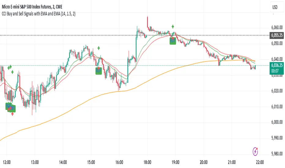
CCI Buy and Sell Signals with 20/30 EMACCI Buy and Sell Signals with EMA and ATR Stop Loss/Take Profit
This indicator is designed to identify buy and sell signals based on a combination of the Commodity Channel Index (CCI) and Exponential Moving Averages (EMA). It also includes an optional ATR-based stop loss and take profit system, which is useful for traders who want to manage their trades with dynamic risk levels.
Features:
CCI Buy and Sell Signals:
Buy Signal: A buy signal is triggered when the CCI crosses up through -100 (from an oversold condition), the 20-period EMA is above the 30-period EMA, and the price is above the 200-period EMA. This suggests that the market is entering an upward trend.
Sell Signal: A sell signal is triggered when the CCI crosses down through +100 (from an overbought condition), the 20-period EMA is below the 30-period EMA, and the price is below the 200-period EMA. This suggests that the market is entering a downward trend.
Exponential Moving Averages (EMA):
The script plots three EMAs:
20-period EMA (Green): Used to identify short-term trends.
30-period EMA (Red): Used to capture medium-term trends.
200-period EMA (Orange): A long-term trend filter, with the price above it generally indicating bullish conditions and below it indicating bearish conditions.
ATR-Based Stop Loss and Take Profit:
Optional Feature: The ATR (Average True Range) indicator can be used to set stop loss and take profit levels based on market volatility.
Stop Loss: Set at a multiple of the ATR below the entry price for long positions and above the entry price for short positions.
Take Profit: Set at a multiple of the ATR above the entry price for long positions and below the entry price for short positions.
Customizable: You can adjust the ATR length, Stop Loss Multiplier, and Take Profit Multiplier through the settings.
Dots: The stop loss and take profit levels are plotted as dots on the chart when the ATR feature is enabled.
Alert Conditions:
Buy Signal Alert: Triggered when a buy signal occurs based on CCI crossing up -100 and other conditions being met.
Sell Signal Alert: Triggered when a sell signal occurs based on CCI crossing down +100 and other conditions being met.
Any Signal Alert: This is a combined alert that triggers for either a buy or sell signal. It helps you stay updated on both types of signals simultaneously.
How to Use:
The indicator will plot buy and sell arrows on the chart, giving clear entry points for trades based on CCI and EMA conditions.
The ATR stop loss and take profit dots (when enabled) provide automatic risk management levels, adjusting dynamically with market volatility.
Traders can customize the ATR settings to fine-tune their stop loss and take profit levels, making this strategy adaptable to different trading styles and market conditions.
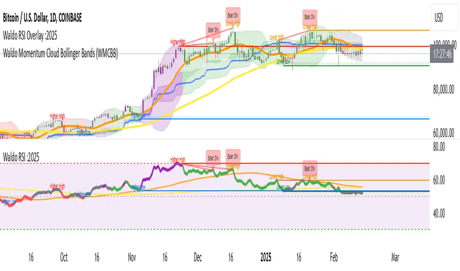
Waldo RSI :oWaldo RSI :o Indicator Guide
The Waldo RSI :o indicator is designed to complement the "Waldo RSI Overlay :o" by providing an RSI-based analysis on TradingView, focusing on macro shifts in market trends. Here's a comprehensive guide on how to use this indicator:
Key Features:
RSI Settings:
RSI Source: Choose from ON RSI, ON HIGH, ON LOW, ON CLOSE, or ON OPEN to determine how RSI calculates pivots.
RSI Settings:
Source: Default is (H+L)/2, but you can select any price for RSI calculation.
Length: Default RSI length is 7, which can be adjusted for sensitivity.
Trend Lines:
Show Trend Lines: Option to display trend lines based on RSI pivot points.
Zigzag Length: Determines pivot point sensitivity.
Confirm Length: Validates pivot points (default is 3).
Colors: Customize colors for Higher Highs (HH), Lower Highs (LH), Higher Lows (HL), and Lower Lows (LL) on the RSI.
Label Size and Line Width: Adjust the appearance of labels and lines.
Divergences:
Classic Divergences:
Show Classic Div: Toggle to reveal divergences where RSI and price move in opposite directions.
Colors: Set different colors for bullish and bearish divergence indicators.
Transparency and Line Width: Control the visual impact of divergence signals.
Hidden Divergences:
Similar settings for identifying hidden divergences, suggest trend continuation.
Breakout/Breakdown:
Show Breakout/Breakdown: Generates signals for RSI breakouts or breakdowns, used by "Waldo RSI Overlay :o" for visual chart signals.
Overbought/Oversold Zones:
Show Overbought and OverSold Zones: Highlights when RSI goes above 70 (overbought) or below 30 (oversold).
Moving Averages on RSI:
The default Moving Average (MA) settings are tailored to capture macro shifts in market trends:
Show Moving Averages: Option to overlay two MAs on the RSI for trend confirmation:
Fast RSI MA:
RSI Period: 50 (this is the period over which the RSI is calculated).
MA Length: 50 (the number of periods used for the moving average of the RSI).
Slow RSI MA:
RSI Period: 50 (same as fast for consistency in RSI calculation).
MA Length: 200 (longer term for capturing broader trends).
Crossover Signals: The RSI changes color from red to green based on these moving average crossovers:
When the Fast MA (50 period) crosses above the Slow MA (200 period), the RSI turns green, indicating potential bullish conditions or momentum shift.
Conversely, when the Fast MA crosses below the Slow MA, the RSI turns red, suggesting bearish conditions or a shift back towards a downtrend.
This 50-period RSI crossover setting is used to identify overall macro shifts in the market, providing a clear visual cue for traders looking at longer-term trends.
Ghost Lines (Optional):
Ghost Lines: Option to limit how far RSI trend lines extend, helping to keep the chart less cluttered.
How to Use the Indicator:
Setup:
Configure RSI by choosing the source and setting the length to match your trading style.
Set the zigzag and confirm lengths for appropriate pivot detection.
Trend Analysis:
Monitor the RSI for trend changes using the colored trend lines and labels.
Divergence Detection:
Look for RSI and price divergences to anticipate potential reversals or continuations.
Breakout/Breakdown:
Use these signals in conjunction with "Waldo RSI Overlay :o" for price action confirmation.
Overbought/Oversold:
Identify when the market might be due for a correction or continued momentum.
Moving Averages:
Focus on the color changes in RSI to understand macro trend shifts with the default 50/200 period setup.
Ghost Lines:
Enable for a cleaner chart if you don't need trend lines extending indefinitely.
Usage Tips:
Combine with other indicators for confirmation, as no single tool is foolproof.
Adjust settings to suit different market conditions or trading timeframes.
Use in tandem with "Waldo RSI Overlay :o" for a full trading signal system.
Remember, trading involves significant risk, and historical data does not guarantee future performance. Use this indicator as part of a broader trading strategy.
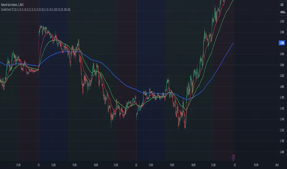
Dynamic Time Zone EMA with Candle Trend AnalysisCandleTrend TZ is a powerful analytical tool that integrates time zones, exponential moving averages (EMA), and custom candle coloring based on trend direction. This indicator is ideal for traders looking to analyze market trends within specific time sessions effectively.
Key Features:
Time Zones:
Divides the chart into four distinct time intervals, each highlighted with a unique background color.
Fully customizable start and end times for each interval, allowing for adaptation to various trading schedules.
Exponential Moving Averages (EMA):
Displays three EMAs with user-defined lengths:
EMA 200 (blue) for long-term trends.
EMA 50 (green) for medium-term trends.
EMA 20 (red) for short-term trends.
Helps identify trend direction and strength.
Custom Candle Coloring:
Utilizes smoothed Heiken Ashi and Triple EMA (TEMA) calculations for enhanced candle coloring:
Green candles indicate an upward trend.
Red candles signal a downward trend.
Filters out market noise, providing a clear visual representation of market dynamics.
Customization Options:
Time Zones:
Adjustable start and end times for each of the four sessions:
Input hour and minute for start and end times (e.g., Interval 1 Start/End Hour/Minute).
Background colors are pre-defined but can be modified in the code.
EMAs:
User-defined lengths for each EMA:
EMA 200 Length (default: 200)
EMA 50 Length (default: 50)
EMA 20 Length (default: 20)
TEMA Settings:
Parameters for trend smoothing:
TEMA Length (default: 55)
EMA Length (default: 60)
Use Cases:
Intraday Session Analysis:
Use time zones to differentiate between morning, afternoon, and evening market activity.
The background colors make it easy to track session-specific trends.
Trend Trading:
Analyze EMA crossings and their slopes to confirm market direction.
Green candles indicate buying opportunities, while red candles highlight selling signals.
Noise Reduction:
TEMA smoothing removes market noise, allowing you to focus on the primary market trend.
Adaptation to Custom Strategies:
By adjusting time intervals, you can tailor the indicator to specific trading styles or market conditions.
Benefits:
Versatility for both trending and sideways markets.
Intuitive and user-friendly setup.
Suitable for traders of all skill levels, from beginners to professionals.
CandleTrend TZ is an indispensable tool for understanding market dynamics, enhancing your trading precision, and making well-informed decisions. 🚀
Combined Multi-Timeframe EMA OscillatorThis script aims to visualize the strength of bullish or bearish trends by utilizing a mix of 200 EMA across multiple timeframes. I've observed that when the multi-timeframe 200 EMA ribbon is aligned and expanding, the uptrend usually lasts longer and is safer to enter at a pullback for trend continuation. Similarly, when the bands are expanding in reverse order, the downtrend holds longer, making it easier to sell the pullbacks.
In this script, I apply a purely empirical and experimental method: a) Ranking the position of each of the above EMAs and turning it into an oscillator. b) Taking each 200 EMA on separate timeframes, turning it into a stochastic-like oscillator, and then averaging them to compute an overall stochastic.
To filter a bullish signal, I use the bullish crossover between these two aggregated oscillators (default: yellow and blue on the chart) which also plots a green shadow area on the screen and I look for buy opportunities/ ignore sell opportunities while this signal is bullish. Similarly, a bearish crossover gives us a bearish signal which also plots a red shadow area on the screen and I only look for sell opportunities/ ignore any buy opportunities while this signal is bearish.
Note that directly buying the signal as it prints can lead to suboptimal entries. The idea behind the above is that these crossovers point on average to a stronger trend; however, a trade should be initiated on the pullbacks with confirmation from momentum and volume indicators and in confluence with key areas of support and resistance and risk management should be used in order to protect your position.
Disclaimer: This script does not constitute certified financial advice, the current work is purely experimental, use at your own discretion.

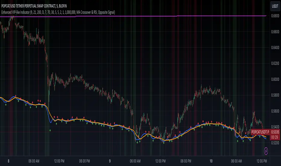
Enhanced VIP-like IndicatorSettings Breakdown Tutorial: Optimizing a Trading Strategy
This guide explains the key trading strategy settings and how to customize them based on your trading style and goals. Each parameter is essential for tailoring the strategy to market conditions and your risk appetite.
1. Short Moving Average Length (Default: 9)
• Purpose: Tracks short-term trends using a small number of candles.
• Settings Tips:
• Smaller Values (e.g., 9): Quickly react to price changes, useful for fast-moving markets.
• Larger Values (e.g., 12-15): Generate smoother signals for less volatile trades.
2. Long Moving Average Length (Default: 21)
• Purpose: Identifies long-term trends.
• Settings Tips:
• Higher Values (e.g., 50): Spot broader trends at the expense of slower signals.
• Trend Analysis: The interaction of short and long MAs helps determine bullish or bearish trends (e.g., bullish when short MA crosses above long MA).
3. Higher Timeframe MA Length (Default: 200)
• Purpose: Filters long-term trends on a higher timeframe (e.g., daily).
• Settings Tips:
• 200 Periods: Standard for defining bullish (price above) or bearish (price below) markets.
• Adjustable: Use 100 for faster responses or stick with 200 for reliability.
4. Higher Timeframe (Default: 1 Day)
• Purpose: Defines the timeframe for the higher moving average.
• Settings Tips:
• Shorter Timeframes (e.g., 4 Hours): More frequent trading signals.
• Daily Timeframe: Best for swing trading and identifying macro trends.
5. RSI Length (Default: 14)
• Purpose: Measures momentum over a specific number of candles.
• Settings Tips:
• Lower Values (e.g., 7): More sensitive to price changes, ideal for quick trades.
• Higher Values (e.g., 20): Smooth signals for more stable markets.
6. RSI Overbought (70) and Oversold (30) Levels
• Purpose: Marks thresholds for overbought and oversold conditions.
• Settings Tips:
• Stricter Levels (e.g., 80/20): Fewer, higher-quality signals.
• Looser Levels (e.g., 65/35): More frequent signals, suitable for active trading.
7. Pivot Left Bars (5) and Pivot Right Bars (5)
• Purpose: Confirms pivot points (support/resistance) based on surrounding candles.
• Settings Tips:
• Higher Values (e.g., 10): Stronger but less frequent pivot points.
• Lower Values: More responsive, for traders seeking quick pivots.
8. Take Profit Percentage (Default: 2%)
• Purpose: Defines the profit level to exit trades.
• Settings Tips:
• Higher Values (e.g., 5%): For swing traders holding positions longer.
• Lower Values (e.g., 1%): For scalpers focusing on quick trades.
9. Minimum Volume (Default: 1,000,000)
• Purpose: Ensures sufficient liquidity for trading.
• Settings Tips:
• Lower Values: For lower-volume markets.
• Higher Values: Reduces risk in high-liquidity assets.
10. Stop Loss Percentage (Default: 1%)
• Purpose: Sets the maximum acceptable loss per trade.
• Settings Tips:
• Lower Values (e.g., 0.5%): Reduces risk, suited for conservative trading.
• Higher Values (e.g., 2%): Allows more price fluctuation, ideal for volatile markets.
11. Entry Conditions
• Options:
• MA Crossover & RSI: Combines trend-following and momentum for well-rounded signals.
• Pivot Breakout: Focuses on support/resistance breakouts for high-impact trades.
• Settings Tips:
• Trend-Following Traders: Use MA Crossover & RSI.
12. Exit Conditions
• Options:
• Opposite Signal: Exits when the trade’s opposite condition occurs (e.g., bullish to bearish).
• Fixed Take Profit/Stop Loss: Exits based on predefined profit/loss thresholds.
• Settings Tips:
• Opposite Signal: Ideal for trend-following strategies.
Summary
Customizing these settings aligns the strategy with your trading goals. Test configurations in a demo environment before live trading to refine the approach and optimize results. Always balance profit potential with risk management.
• Fixed Levels: Better for strict risk management.
• Breakout Traders: Opt for Pivot Breakout.
Volume-Based RSI Color Indicator with MAsVolume-Based RSI Color Indicator with MAs
Overview
This script combines the Relative Strength Index (RSI) with volume analysis to provide an enhanced perspective on market conditions. By dynamically coloring the RSI line based on overbought/oversold conditions and volume thresholds, this indicator helps traders quickly identify high-probability reversal zones. Additionally, it incorporates short-term and long-term moving averages (MAs) of the RSI for trend analysis, making it a versatile tool for scalping and swing trading strategies.
Key Features
Dynamic RSI Color Coding:
The RSI line changes color based on two conditions:
Overbought/High Volume: RSI is above the overbought threshold (default: 70) and volume exceeds the average volume by a user-defined multiplier (default: 2.0). The line turns red, indicating potential reversal zones.
Oversold/High Volume: RSI is below the oversold threshold (default: 30) and volume exceeds the average volume by the multiplier. The line turns green, suggesting potential buying opportunities.
Neutral Conditions: Default blue color for all other scenarios.
Volume Integration:
Unlike standard RSI indicators, this script incorporates volume data to refine signals, helping traders avoid false signals in low-volume environments.
RSI Moving Averages:
Two moving averages of the RSI (short-term and long-term) provide trend context:
200-period MA: Highlights the long-term trend in RSI values.
20-period MA: Shows short-term fluctuations for quick decision-making.
Both MAs can be calculated using Simple or Exponential methods, giving users flexibility.
Visual Aids:
Horizontal lines at the overbought (70) and oversold (30) levels help define the boundaries of expected price action extremes.
How It Works
The script calculates the RSI over a user-defined length (default: 14).
Volume data is compared to its moving average to determine if it exceeds the user-defined high-volume threshold.
When RSI and volume conditions align, the RSI line is dynamically colored to indicate potential overbought/oversold zones.
The RSI moving averages provide additional context to confirm trends or reversals.
How to Use
Identify Reversal Zones:
Look for green RSI signals in oversold conditions to identify potential buying opportunities.
Look for red RSI signals in overbought conditions to identify potential selling opportunities.
Use Moving Averages for Confirmation:
When the RSI is above its 200-period MA, the long-term trend is bullish; consider only long trades.
When the RSI is below its 200-period MA, the trend is bearish; consider only short trades.
Combine with Other Tools:
This indicator works best when used alongside price action analysis, candlestick patterns, or support/resistance levels.
Originality
This script is unique in combining volume analysis with RSI and RSI-specific moving averages. While many indicators focus on RSI or volume separately, this script marries these two key metrics to filter out weak signals and improve trade decision accuracy.
Chart Recommendations
Clean Chart: Use this indicator on a clean chart without additional overlays for maximum clarity.
Timeframes: Works well on intraday charts (e.g., 5m, 15m) for scalping and on higher timeframes (e.g., 1H, 4H, Daily) for swing trading.
Disclaimer
This indicator is a tool to aid trading decisions and should not be used in isolation. Always consider other factors such as market conditions, news events, and risk management.
