Supertrend EMA Vol Strategy V5### Supertrend EMA Strategy V5
**Overview**
This is a trend-following strategy designed for cryptocurrency markets like BTC/USD on daily timeframes, combining the Supertrend indicator for dynamic trailing stops with an EMA filter for trend confirmation. It aims to capture strong uptrends while avoiding counter-trend trades, with optional volume filtering for high-conviction entries and ATR-based stop-loss to manage risk. Ideal for long-only setups in bullish assets, it visually highlights trends with green/red bands and fills for easy interpretation. Backtested on BTC from 2024-2025, it shows potential for outperforming buy-and-hold in trending markets, but always use with proper risk management—past performance isn't indicative of future results.
**Key Features**
- **Supertrend Core**: Uses ATR to plot adaptive uptrend (green) and downtrend (red) lines, flipping on closes beyond prior bands for buy/sell signals.
- **EMA Trend Filter**: Entries require price above the EMA (default 21-period) for longs, ensuring alignment with the broader trend.
- **Volume Confirmation**: Optional filter only allows entries when volume exceeds its EMA (default 20-period), reducing false signals in low-activity periods.
- **Risk Controls**: Built-in ATR-multiplier stop-loss (default 2x) to cap losses; exits on Supertrend flips for trailing profits.
- **Visuals**: Green/red lines and highlighter fills for up/down trends, plus buy/sell labels and circles for signals.
- **Customizable Inputs**: Tweak ATR period (default 10), multiplier (default 3), EMA length, start date, long/short toggles, SL, and volume filter.
- **Alerts**: Built-in for buy/sell and direction changes.
**How to Use**
1. Add to your TradingView chart (e.g., BTC/USD 1D).
2. Adjust inputs: Start with defaults for trend-following; increase multiplier for fewer trades/higher win rate. Enable volume filter for volatile assets.
3. Monitor signals: Green "Buy" for long entries (if close > EMA and conditions met); red "Sell" for exits.
4. Backtest in Strategy Tester: Focus on equity curve, win rate (~50-60% in tests), and drawdown (<15% with SL).
5. Live Trading: Use small position sizes (1-2% risk per trade); combine with your analysis. Shorts disabled by default for bull-biased markets.
Cerca negli script per "2024年5月2日+沪深股市+成交额+新闻"

Bitcoin Logarithmic Growth Curve 2025 Z-Score"The Bitcoin logarithmic growth curve is a concept used to analyze Bitcoin's price movements over time. The idea is based on the observation that Bitcoin's price tends to grow exponentially, particularly during bull markets. It attempts to give a long-term perspective on the Bitcoin price movements.
The curve includes an upper and lower band. These bands often represent zones where Bitcoin's price is overextended (upper band) or undervalued (lower band) relative to its historical growth trajectory. When the price touches or exceeds the upper band, it may indicate a speculative bubble, while prices near the lower band may suggest a buying opportunity.
Unlike most Bitcoin growth curve indicators, this one includes a logarithmic growth curve optimized using the latest 2024 price data, making it, in our view, superior to previous models. Additionally, it features statistical confidence intervals derived from linear regression, compatible across all timeframes, and extrapolates the data far into the future. Finally, this model allows users the flexibility to manually adjust the function parameters to suit their preferences.
The Bitcoin logarithmic growth curve has the following function:
y = 10^(a * log10(x) - b)
In the context of this formula, the y value represents the Bitcoin price, while the x value corresponds to the time, specifically indicated by the weekly bar number on the chart.
How is it made (You can skip this section if you’re not a fan of math):
To optimize the fit of this function and determine the optimal values of a and b, the previous weekly cycle peak values were analyzed. The corresponding x and y values were recorded as follows:
113, 18.55
240, 1004.42
451, 19128.27
655, 65502.47
The same process was applied to the bear market low values:
103, 2.48
267, 211.03
471, 3192.87
676, 16255.15
Next, these values were converted to their linear form by applying the base-10 logarithm. This transformation allows the function to be expressed in a linear state: y = a * x − b. This step is essential for enabling linear regression on these values.
For the cycle peak (x,y) values:
2.053, 1.268
2.380, 3.002
2.654, 4.282
2.816, 4.816
And for the bear market low (x,y) values:
2.013, 0.394
2.427, 2.324
2.673, 3.504
2.830, 4.211
Next, linear regression was performed on both these datasets. (Numerous tools are available online for linear regression calculations, making manual computations unnecessary).
Linear regression is a method used to find a straight line that best represents the relationship between two variables. It looks at how changes in one variable affect another and tries to predict values based on that relationship.
The goal is to minimize the differences between the actual data points and the points predicted by the line. Essentially, it aims to optimize for the highest R-Square value.
Below are the results:
snapshot
snapshot
It is important to note that both the slope (a-value) and the y-intercept (b-value) have associated standard errors. These standard errors can be used to calculate confidence intervals by multiplying them by the t-values (two degrees of freedom) from the linear regression.
These t-values can be found in a t-distribution table. For the top cycle confidence intervals, we used t10% (0.133), t25% (0.323), and t33% (0.414). For the bottom cycle confidence intervals, the t-values used were t10% (0.133), t25% (0.323), t33% (0.414), t50% (0.765), and t67% (1.063).
The final bull cycle function is:
y = 10^(4.058 ± 0.133 * log10(x) – 6.44 ± 0.324)
The final bear cycle function is:
y = 10^(4.684 ± 0.025 * log10(x) – -9.034 ± 0.063)
The main Criticisms of growth curve models:
The Bitcoin logarithmic growth curve model faces several general criticisms that we’d like to highlight briefly. The most significant, in our view, is its heavy reliance on past price data, which may not accurately forecast future trends. For instance, previous growth curve models from 2020 on TradingView were overly optimistic in predicting the last cycle’s peak.
This is why we aimed to present our process for deriving the final functions in a transparent, step-by-step scientific manner, including statistical confidence intervals. It's important to note that the bull cycle function is less reliable than the bear cycle function, as the top band is significantly wider than the bottom band.
Even so, we still believe that the Bitcoin logarithmic growth curve presented in this script is overly optimistic since it goes parly against the concept of diminishing returns which we discussed in this post:
This is why we also propose alternative parameter settings that align more closely with the theory of diminishing returns."
Now with Z-Score calculation for easy and constant valuation classification of Bitcoin according to this metric.
Created for TRW

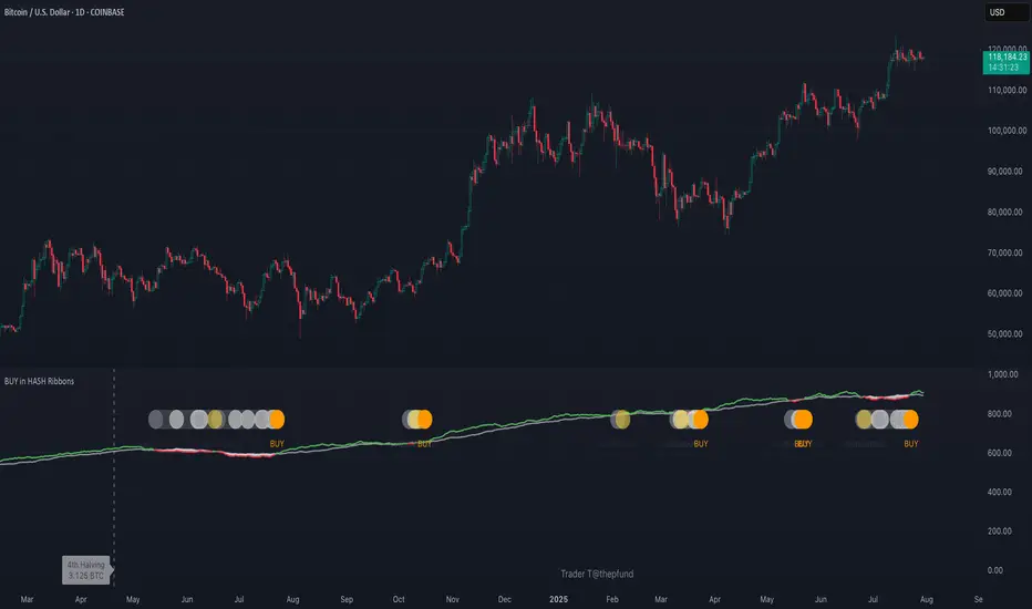
BUY in HASH RibbonsHash Ribbons Indicator (BUY Signal)
A TradingView Pine Script v6 implementation for identifying Bitcoin miner capitulation (“Springs”) and recovery phases based on hash rate data. It marks potential low-risk buying opportunities by tracking short- and long-term moving averages of the network hash rate.
⸻
Key Features
• Hash Rate SMAs
• Short-term SMA (default: 30 days)
• Long-term SMA (default: 60 days)
• Phase Markers
• Gray circle: Short SMA crosses below long SMA (start of capitulation)
• White circles: Ongoing capitulation, with brighter white when the short SMA turns upward
• Yellow circle: Short SMA crosses back above long SMA (end of capitulation)
• Orange circle: Buy signal once hash rate recovery aligns with bullish price momentum (10-day price SMA crosses above 20-day price SMA)
• Display Modes
• Ribbons: Plots the two SMAs as colored bands—red for capitulation, green for recovery
• Oscillator: Shows the percentage difference between SMAs as a histogram (red for negative, blue for positive)
• Optional Overlays
• Bitcoin halving dates (2012, 2016, 2020, 2024) with dashed lines and labels
• Raw hash rate data in EH/s
• Alerts
• Configurable alerts for capitulation start, recovery, and buy signals
⸻
How It Works
1. Data Source: Fetches daily hash rate values from a selected provider (e.g., IntoTheBlock, Quandl).
2. Capitulation Detection: When the 30-day SMA falls below the 60-day SMA, miners are likely capitulating.
3. Recovery Identification: A rising 30-day SMA during capitulation signals miner recovery.
4. Buy Signal: Confirmed when the hash rate recovery coincides with a bullish shift in price momentum (10-day price SMA > 20-day price SMA).
⸻
Inputs
Hash Rate Short SMA: 30 days
Hash Rate Long SMA: 60 days
Plot Signals: On
Plot Halvings: Off
Plot Raw Hash Rate: Off
⸻
Considerations
• Timeframe: Best applied on daily charts to capture meaningful miner behavior.
• Data Reliability: Ensure the chosen hash rate source provides consistent, gap-free data.
• Risk Management: Use alongside other technical indicators (e.g., RSI, MACD) and fundamental analysis.
• Backtesting: Evaluate performance over different market cycles before live deployment.
Portfolio Tracker ARJO (V-01)Portfolio Tracker ARJO (V-01)
This indicator is a user-friendly portfolio tracking tool designed for TradingView charts. It overlays a customizable table on your chart to monitor up to 15 stocks or symbols in your portfolio. It calculates real-time metrics like current market price (CMP), gains/losses, and stoploss breaches, helping you stay on top of your investments without switching between multiple charts. The table uses color-coding for quick visual insights: green for profits, red for losses, and highlights breached stoplosses in red for alerts. It also shows portfolio-wide totals for overall performance.
Key Features
Supports up to 15 Symbols: Enter stock tickers (e.g., NSE:RELIANCE or BSE:TCS) with details like buy price, date, units, and stoploss.
Symbol: The stock ticker and description.
Buy Date: When you purchased it.
Units: Number of shares/units held.
Buy Price: Your entry price.
Stop Loss: Your set stoploss level (highlighted in red if breached by CMP).
CMP: Current market price (fetched from the chart's timeframe).
% Gain/Loss: Percentage change from buy price (color-coded: green for positive, red for negative).
Gain/Loss: Total monetary gain/loss based on units.
Optional Timeframe Columns: Toggle to show % change over 1 Week (1W), 1 Month (1M), 3 Months (3M), and 6 Months (6M) for historical performance.
Portfolio Summary: At the top of the table, see total % gain/loss and absolute gain/loss for your entire portfolio.
Visual Customizations: Adjust table position (e.g., Top Right), size, colors for positive/negative values, and intensity cutoff for gradients.
Benchmark Index-Based Header: The title row's background color reflects NIFTY's weekly trend (green if above 10-week SMA, red if below) for market context.
Benchmark Index-Based Header: The title row's background color reflects NIFTY's weekly trend (green if above 10-week SMA, red if below) for market context.
How to Use It: Step-by-Step Guide
Add the Indicator to Your Chart: Search for "Portfolio Tracker ARJO (V-01)" in TradingView's indicator library and add it to any chart (preferably Daily timeframe for accuracy).
Input Your Portfolio Symbols:
Open the indicator settings (gear icon).
In the "Symbol 1" to "Symbol 15" groups, fill in:
Symbol: Enter the ticker (e.g., NSE:INFY).
Year/Month/Day: Select your buy date (e.g., 2024-07-01).
Buy Price: Your purchase price per unit.
Stoploss: Your exit price if things go south.
Units: How many shares you own.
Only fill what you need—leave extras blank. The table auto-adjusts to show only entered symbols.
Customize the Table (Optional):
In "Table settings":
Choose position (e.g., Top Right) and size (% of chart).
Toggle "Show Timeframe Columns" to add 1W/1M/3M/6M performance.
In "Color settings":
Pick colors for positive (green) and negative (red) cells.
Set "Color intensity cutoff (%)" to control how strong the colors get (e.g., 10% means changes above 10% max out the color).
Interpret the Table on Your Chart:
The table appears overlaid—scan rows for each symbol's stats.
Look at colors: Greener = better gains; redder = bigger losses.
Check CMP cell: Red means stoploss breached—consider selling!
Portfolio Gain/Loss at the top gives a quick overall health check.
For Best Results:
Use on a Daily chart to avoid CMP errors (the script will warn if on Weekly/Monthly).
Refresh the chart or wait for a new bar if data doesn't update immediately.
For Indian stocks, prefix with NSE: or BSE: (e.g., BSE:RELIANCE).
This is for tracking only—not trading signals. Combine with your strategy.
If no symbols show, ensure inputs are valid (e.g., buy price > 0, valid date).
Finally, this tool makes it quite easy for beginners to track their portfolios, while also giving advanced traders powerful and customizable insights. I'd love to hear your feedback—happy trading!

Auto Intelligence Selective Moving Average(AI/MA)# 🤖 Auto Intelligence Moving Average Strategy (AI/MA)
**AI/MA** is a state-adaptive moving average crossover strategy designed to **maximize returns from golden cross / death cross logic** by intelligently switching between different MA types and parameters based on market conditions.
---
## 🎯 Objective
To build a moving average crossover strategy that:
- **Adapts dynamically** to market regimes (trend vs range, rising vs falling)
- **Switches intelligently** between SMA, EMA, RMA, and HMA
- **Maximizes cumulative return** under realistic backtesting
---
## 🧪 materials amd methods
- **MA Types Considered**: SMA, EMA, RMA, HMA
- **Parameter Ranges**: Periods from 5 to 40
- **Market Conditions Classification**:
- Based on the slope of a central SMA(20) line
- And the relative position of price to the central line
- Resulting in 4 regimes: A (Bull), B (Pullback), C (Rebound), D (Bear)
- **Optimization Dataset**:
- **Bybit BTCUSDT.P**
- **1-hour candles**
- **2024 full-year**
- **Search Process**:
- **Random search**: 200 parameter combinations
- Evaluated by:
- `Cumulative PnL`
- `Sharpe Ratio`
- `Max Drawdown`
- `R² of linear regression on cumulative PnL`
- **Implementation**:
- Optimization performed in **Python (Pandas + Matplotlib + Optuna-like logic)**
- Final parameters ported to **Pine Script (v5)** for TradingView backtesting
---
## 📈 Performance Highlights (on optimization set)
| Timeframe | Return (%) | Notes |
|-----------|------------|----------------------------|
| 6H | +1731% | Strongest performance |
| 1D | +1691% | Excellent trend capture |
| 12H | +1438% | Balance of trend/range |
| 5min | +27.3% | Even survives scalping |
| 1min | +9.34% | Robust against noise |
- Leverage: 100x
- Position size: 100%
- Fees: 0.055%
- Margin calls: **none** 🎯
---
## 🛠 Technology Stack
- `Python` for data handling and optimization
- `Pine Script v5` for implementation and visualization
- Fully state-aware strategy, modular and extendable
---
## ✨ Final Words
This strategy is **not curve-fitted**, **not over-parameterized**, and has been validated across multiple timeframes. If you're a fan of dynamic, intelligent technical systems, feel free to use and expand it.
💡 The future of simple-yet-smart trading begins here.

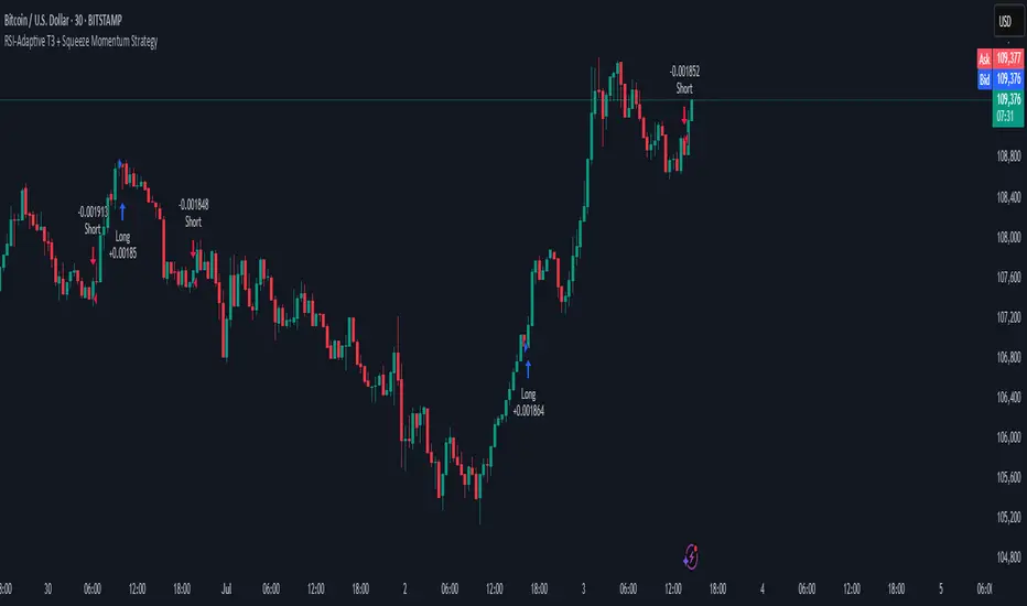
RSI-Adaptive T3 + Squeeze Momentum Strategy✅ Strategy Guide: RSI-Adaptive T3 + Squeeze Momentum Strategy
📌 Overview
The RSI-Adaptive T3 + Squeeze Momentum Strategy is a dynamic trend-following strategy based on an RSI-responsive T3 moving average and Squeeze Momentum detection .
It adapts in real-time to market volatility to enhance entry precision and optimize risk.
⚠️ This strategy is provided for educational and research purposes only.
Past performance does not guarantee future results.
🎯 Strategy Objectives
The main objective of this strategy is to catch the early phase of a trend and generate consistent entry signals.
Designed to be intuitive and accessible for traders from beginner to advanced levels.
✨ Key Features
RSI-Responsive T3: T3 length dynamically adjusts according to RSI values for adaptive trend detection
Squeeze Momentum: Combines Bollinger Bands and Keltner Channels to identify trend buildup phases
Visual Triggers: Entry signals are generated from T3 crossovers and momentum strength after squeeze release
📊 Trading Rules
Long Entry:
When T3 crosses upward, momentum is positive, and the squeeze has just been released.
Short Entry:
When T3 crosses downward, momentum is negative, and the squeeze has just been released.
Exit (Reversal):
When the opposite condition to the entry is triggered, the position is reversed.
💰 Risk Management Parameters
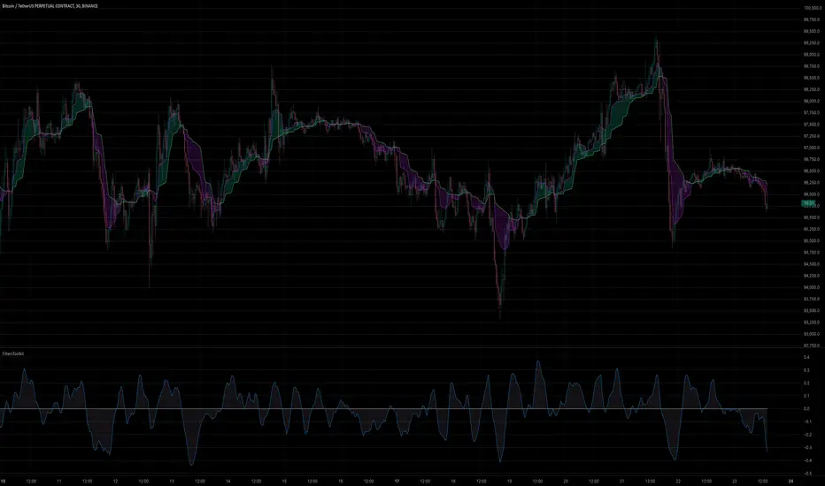
Pair & Timeframe: BTC/USD (30-minute chart)
Capital (simulated): $30,00
Order size: `$100` per trade (realistic, low-risk sizing)
Commission: 0.02%
Slippage: 2 pips
Risk per Trade: 5%
Number of Trades (backtest period): 181
📊 Performance Overview
Symbol: BTC/USD
Timeframe: 30-minute chart
Date Range: January 1, 2024 – July 3, 2025
Win Rate: 47.8%
Profit Factor: 2.01
Net Profit: 173.16 (units not specified)
Max Drawdown: 5.77% or 24.91 (0.79%)
⚙️ Indicator Parameters
Indicator Name: RSI-Adaptive T3 + Squeeze Momentum
RSI Length: 14
T3 Min Length: 5
T3 Max Length: 50
T3 Volume Factor: 0.7
BB Length: 27 (Multiplier: 2.0)
KC Length: 20 (Multiplier: 1.5, TrueRange enabled)
🖼 Visual Support
T3 slope direction, squeeze status, and momentum bars are visually plotted on the chart,
providing high clarity for quick trend analysis and execution.
🔧 Strategy Improvements & Uniqueness
Inspired by the RSI Adaptive T3 by ChartPrime and Squeeze Momentum Indicator by LazyBear ,
this strategy fuses both into a hybrid trend-reversal and momentum breakout detection system .
Compared to traditional trend-following methods, it excels at capturing early trend signals with greater sensitivity .
✅ Summary
The RSI-Adaptive T3 + Squeeze Momentum Strategy combines momentum detection with volatility-responsive risk management.
With a strong balance between visual clarity and practicality, it serves as a powerful tool for traders seeking high repeatability.
⚠️ This strategy is based on historical data and does not guarantee future profits.
Always use appropriate risk management when applying it.
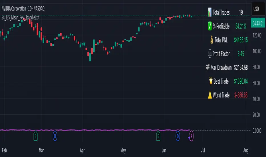
S4_IBS_Mean_Rev_3candleExitOverview:
This is a rules-based, mean reversion strategy designed to trade pullbacks using the Internal Bar Strength (IBS) indicator. The system looks for oversold conditions based on IBS, then enters long trades , holding for a maximum of 3 bars or until the trade becomes profitable.
The strategy includes:
✅ Strict entry rules based on IBS
✅ Hardcoded exit conditions for risk management
✅ A clean visual table summarizing key performance metrics
How It Works:
1. Internal Bar Strength (IBS) Setup:
The IBS is calculated using the previous bar’s price range:
IBS = (Previous Close - Previous Low) / (Previous High - Previous Low)
IBS values closer to 0 indicate price is near the bottom of the previous range, suggesting oversold conditions.
2. Entry Conditions:
IBS must be ≤ 0.25, signaling an oversold setup.
Trade entries are only allowed within a user-defined backtest window (default: 2024).
Only one trade at a time is permitted (long-only strategy).
3. Exit Conditions:
If the price closes higher than the entry price, the trade exits with a profit.
If the trade has been open for 3 bars without showing profit, the trade is forcefully exited.
All trades are closed automatically at the end of the backtest window if still open.
Additional Features:
📊 A real-time performance metrics table is displayed on the chart, showing:
- Total trades
- % of profitable trades
- Total P&L
- Profit Factor
- Max Drawdown
- Best/Worst trade performance
📈 Visual markers indicate trade entries (green triangle) and exits (red triangle) for easy chart interpretation.
Who Is This For?
This strategy is designed for:
✅ Traders exploring systematic mean reversion approaches
✅ Those who prefer strict, rules-based setups with no subjective decision-making
✅ Traders who want built-in performance tracking directly on the chart
Note: This strategy is provided for educational and research purposes. It is a backtested model and past performance does not guarantee future results. Users should paper trade and validate performance before considering real capital.
High Low Levels by JZCustom High Low Levels Indicator - features
Clearly plotted high and low levels for specific trading sessions. This indicator provides visual representations of key price levels during various trading periods. Below are the main features and benefits of this indicator:
1. Display high and low levels for each session
- previous day high/low: display the high and low from the previous day, giving you a better understanding of how the price moves compared to the prior day.
- asia, london, and custom sessions: track the high and low levels for the major trading sessions (asian and london) and two custom user-defined sessions.
2. Complete line and label customization
- custom line appearance: choose the color, line style (solid, dashed, dotted), and line thickness for each trading session. you can also decide if the lines should extend beyond the current price action.
- custom labels: define your own label texts for each custom session. this way, you can label the levels precisely and easily track price movements.
3. Define your own trading sessions
- add up to two custom sessions (custom and custom 2), which can be defined using precise start and end times (hour and minute).
- each custom session allows you to specify the label text for the high and low levels, enabling you to easily differentiate different parts of the day on the chart.
4. Clear and intuitive design
- grouped settings: all settings are grouped based on trading sessions, so you can easily customize every aspect of the visual representation.
- simple toggle on/off: you can easily enable or disable each line (previous day, asia, london, custom 1, custom 2). this allows you to keep your chart clean and focus only on the important levels you need at any moment.
5. Flexible time zones
- time zone settings: set the time zone (utc, europe/london, america/new_york, asia/tokyo) to properly align the timeframes for each level depending on the market you're focusing on.
6. Automatic cleanup of old lines and labels
- old levels removal: automatically remove old lines and labels to prevent clutter on your chart. this ensures that only current, relevant levels for each trading day or session are displayed.
7. Precise plotting and line extension
- accurate level markings: the indicator calculates the precise times when the high and low levels were reached and plots lines that visually represent these levels.
- line extension options: you have the option to extend the high/low lines beyond their point of calculation, which helps with identifying price action trends beyond the current period.
Dec 7, 2024
Release Notes
Changes and Improvements for Users:
1. Customizable Offset for Lines and Labels:
- A new input, `Line and Label Offset`, allows users to control how far the lines and their associated text labels extend. This ensures the labels and lines remain aligned and can be adjusted as needed.
2. Unified Offset Control:
- The same offset value is applied to all types of lines and labels (e.g., Previous Day High/Low, Asia High/Low, London High/Low, and custom sessions). Users can change this in one place to affect the entire script consistently.
3. Enhanced Flexibility:
- Users now have more control over the appearance and position of their lines and labels, making the indicator adaptable to different chart setups and personal preferences.
These updates aim to enhance user convenience and customization, ensuring a more tailored charting experience.

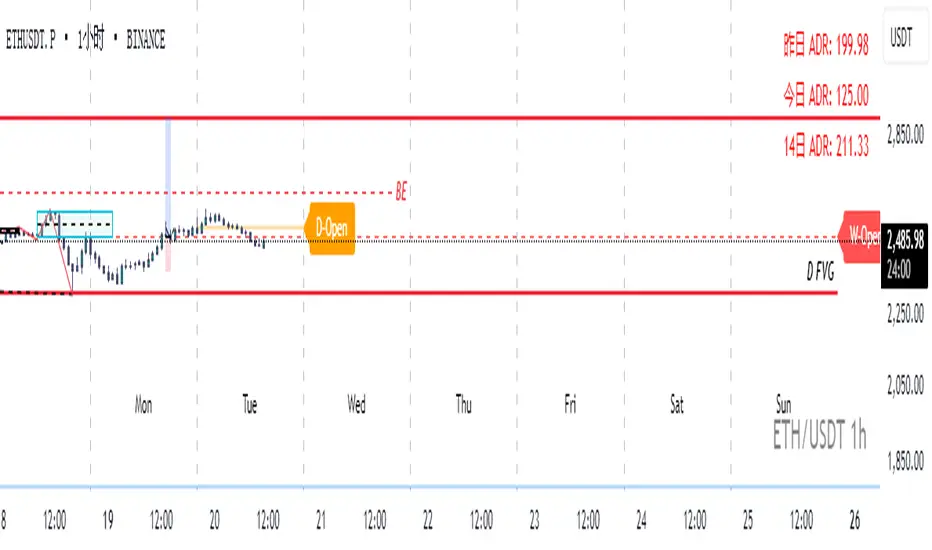
Real-Time Open Levels with Labels + Info TableReal-Time Multi-Timeframe Open Levels with Labels & Info Panel
Overview
This indicator displays real-time opening price levels across multiple timeframes (Monthly, Weekly, Daily, 4H) directly on your chart. It features:
• Dynamic horizontal lines extending through each timeframe period
• Customizable labels with text/colors
• Special 4H line treatment for the last hour (5-min charts only)
• Integrated information panel showing symbol, timeframe, and price changes
! (www.tradingview.com)
*Example showing multiple timeframe levels with labels and info panel*
---
Features & Configuration
1. Monthly Settings
! (www.tradingview.com)
Show Monthly: Toggle visibility of monthly opening price
Color: Semi-transparent blue (#2196F3 at 70% opacity)
Width: 2px line thickness
Style: Solid/Dotted/Dashed
Label: Display "M-Open" text with white text on blue background
2. Weekly Settings
! (www.tradingview.com)
Show Weekly: Toggle weekly opening price visibility
Color: Semi-transparent red (#FF5252 at 70% opacity)
Width: 1px thickness
Style: Dotted by default
Label: "W-Open" text in white on red background
3. Daily Settings
! (www.tradingview.com)
Show Daily: Toggle daily opening price
Color: Amber (#FFA000 at 70% opacity)
Width: 2px thickness
Style: Solid
Label: "D-Open" in white on orange background
---
4. 4-Hour Settings (5-Minute Charts Only)
Special Features for 5-Min Timeframe:
1. Standard 4H Line
• First 3 hours: Green (#4CAF50) dashed line
• Last hour: Bright red solid line (configurable)
• Vertical divider between 3rd/4th hours
2. Configuration Options
• Main 4H Line:
◦ Color/Width/Style for initial 3 hours
◦ Toggle label ("H4-Open") visibility and styling
• Final Hour Enhancement:
*Last Hour Line*
◦ Unique red color and line style
◦ Separate width (1px) and style (Solid)
*Divider Line*
◦ Vertical red dotted line marking last hour
◦ Adjustable position/width/transparency
! (www.tradingview.com)
*4H levels showing 3-hour segment and final hour treatment*
---
5. Info Panel Settings
Positioning:
• Anchor to any chart corner (Top/Bottom + Left/Right combinations)
• Three text sizes: Title (Huge), Change % (Large), Signature (Small)
Display Elements:
• Symbol: Show exchange prefix (e.g., "NASDAQ:")
• Timeframe: Current chart period (e.g., "5m")
• Change %: 24-hour price movement ▲/▼ percentage
• Custom Signature: Add text/username in footer
Styling:
• Semi-transparent white text (#ffffff77)
• Currency pair formatting (e.g., BTC/USD vs BTC-USD)
! (www.tradingview.com)
*Sample info panel with all elements enabled*
---
Usage Tips
1. Multi-Timeframe Context: Use levels to identify key daily/weekly support/resistance
2. 4H Trading: On 5-min charts, watch for price reactions near final hour transition
3. Customization:
• Match line colors to your chart theme
• Use different labels for clarity (e.g., "Weekly Open")
• Disable unused elements to reduce clutter
4. Divider Lines: Helps identify institutional trading periods (hour closes)
---
*Created using Pine Script v6. For optimal performance, use on charts <1H timeframe. ()*
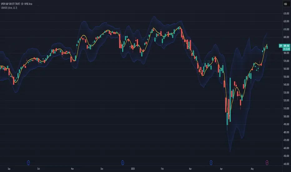
Ehlers Ultimate Bands (UBANDS)UBANDS: ULTIMATE BANDS
🔍 OVERVIEW AND PURPOSE
Ultimate Bands, developed by John F. Ehlers, are a volatility-based channel indicator designed to provide a responsive and smooth representation of price boundaries with significantly reduced lag compared to traditional Bollinger Bands. Bollinger Bands typically use a Simple Moving Average for the centerline and standard deviations from it to establish the bands, both of which can increase lag. Ultimate Bands address this by employing Ehlers' Ultrasmooth Filter for the central moving average. The bands are then plotted based on the volatility of price around this ultrasmooth centerline.
The primary purpose of Ultimate Bands is to offer traders a clearer view of potential support and resistance levels that react quickly to price changes while filtering out excessive noise, aiming for nearly zero lag in the indicator band.
🧩 CORE CONCEPTS
Ultrasmooth Centerline: Employs the Ehlers Ultrasmooth Filter as the basis (centerline) for the bands, aiming for minimal lag and enhanced smoothing.
Volatility-Adaptive Width: The distance between the upper and lower bands is determined by a measure of price deviation from the ultrasmooth centerline. This causes the bands to widen during volatile periods and contract during calm periods.
Dynamic Support/Resistance: The bands serve as dynamic levels of potential support (lower band) and resistance (upper band).
🧮 CALCULATION AND MATHEMATICAL FOUNDATION
Ehlers' Original Concept for Deviation:
John Ehlers describes the deviation calculation as: "The deviation at each data sample is the difference between Smooth and the Close at that data point. The Standard Deviation (SD) is computed as the square root of the average of the squares of the individual deviations."
This describes calculating the Root Mean Square (RMS) of the residuals:
Smooth = UltrasmoothFilter(Source, Length)
Residuals = Source - Smooth
SumOfSquaredResiduals = Sum(Residuals ^2) for i over Length
MeanOfSquaredResiduals = SumOfSquaredResiduals / Length
SD_Ehlers = SquareRoot(MeanOfSquaredResiduals) (This is the RMS of residuals)
Pine Script Implementation's Deviation:
The provided Pine Script implementation calculates the statistical standard deviation of the residuals:
Smooth = UltrasmoothFilter(Source, Length) (referred to as _ehusf in the script)
Residuals = Source - Smooth
Mean_Residuals = Average(Residuals, Length)
Variance_Residuals = Average((Residuals - Mean_Residuals)^2, Length)
SD_Pine = SquareRoot(Variance_Residuals) (This is the statistical standard deviation of residuals)
Band Calculation (Common to both approaches, using their respective SD):
UpperBand = Smooth + (NumSDs × SD)
LowerBand = Smooth - (NumSDs × SD)
🔍 Technical Note: The Pine Script implementation uses a statistical standard deviation of the residuals (differences between price and the smooth average). Ehlers' original text implies an RMS of these residuals. While both measure dispersion, they will yield slightly different values. The Ultrasmooth Filter itself is a key component, designed for responsiveness.
📈 INTERPRETATION DETAILS
Reduced Lag: The primary advantage is the significant reduction in lag compared to standard Bollinger Bands, allowing for quicker reaction to price changes.
Volatility Indication: Widening bands indicate increasing market volatility, while narrowing bands suggest decreasing volatility.
Overbought/Oversold Conditions (Use with caution):
• Price touching or exceeding the Upper Band may suggest overbought conditions.
• Price touching or falling below the Lower Band may suggest oversold conditions.
Trend Identification:
• Price consistently "walking the band" (moving along the upper or lower band) can indicate a strong trend.
• The Middle Band (Ultrasmooth Filter) acts as a dynamic support/resistance level and indicates the short-term trend direction.
Comparison to Ultimate Channel: Ehlers notes that the Ultimate Band indicator does not differ from the Ultimate Channel indicator in any major fashion.
🛠️ USE AND APPLICATION
Ultimate Bands can be used similarly to how Keltner Channels or Bollinger Bands are used for interpreting price action, with the main difference being the reduced lag.
Example Trading Strategy (from John F. Ehlers):
Hold a position in the direction of the Ultimate Smoother (the centerline).
Exit that position when the price "pops" outside the channel or band in the opposite direction of the trade.
This is described as a trend-following strategy with an automatic following stop.
⚠️ LIMITATIONS AND CONSIDERATIONS
Lag (Minimized but Present): While significantly reduced, some minimal lag inherent to averaging processes will still exist. Increasing the Length parameter for smoother bands will moderately increase this lag.
Parameter Sensitivity: The Length and StdDev Multiplier settings are key to tuning the indicator for different assets and timeframes.
False Signals: As with any band indicator, false signals can occur, particularly in choppy or non-trending markets.
Not a Standalone System: Best used in conjunction with other forms of analysis for confirmation.
Deviation Calculation Nuance: Be aware of the difference in deviation calculation (statistical standard deviation vs. RMS of residuals) if comparing directly to Ehlers' original concept as described.
📚 REFERENCES
Ehlers, J. F. (2024). Article/Publication where "Code Listing 2" for Ultimate Bands is featured. (Specific source to be identified if known, e.g., "Stocks & Commodities Magazine, Vol. XX, No. YY").
Ehlers, J. F. (General). Various publications on advanced filtering and cycle analysis. (e.g., "Rocket Science for Traders", "Cycle Analytics for Traders").
OHLCVDataOHLCV Data Power Library
Multi-Timeframe Market Data with Mathematical Precision
📌 Overview
This Pine Script library provides structured OHLCV (Open, High, Low, Close, Volume) data across multiple timeframes using mathematically significant candle counts (powers of 3). Designed for technical analysts who work with fractal market patterns and need efficient access to higher timeframe data.
✨ Key Features
6 Timeframes: 5min, 1H, 4H, 6H, 1D, and 1W data
Power-of-3 Candle Counts: 3, 9, 27, 81, and 243 bars
Structured Data: Returns clean OHLCV objects with all price/volume components
Pine Script Optimized: Complies with all security() call restrictions
📊 Timeframe Functions
pinescript
f_get5M_3() // 3 candles of 5min data
f_get1H_27() // 27 candles of 1H data
f_get1D_81() // 81 candles of daily data
// ... and 27 other combinations
🚀 Usage Example
pinescript
import YourName/OHLCVData/1 as OHLCV
weeklyData = OHLCV.f_get1W_27() // Get 27 weekly candles
latestHigh = array.get(weeklyData, 0).high
plot(latestHigh, "Weekly High")
💡 Ideal For
Multi-timeframe analysis
Volume-profile studies
Fractal pattern detection
Higher timeframe confirmation
⚠️ Note
Replace "YourName" with your publishing username
All functions return arrays of OHLCV objects
Maximum lookback = 243 candles
📜 Version History
1.0 - Initial release (2024)

Stoch_RSI_ChartEnhanced Stochastic RSI Divergence Indicator with VWAP Filter for Charts
This custom indicator builds upon the classic Stochastic RSI to automatically detect both regular and hidden divergences. It’s designed to help traders spot potential market reversals or continuations using two methods for divergence detection (fractal‑ and pivot‑based) while offering optional VWAP filtering for confirmation.
Key Features
Stoch RSI Calculation
The indicator computes a smoothed Stoch RSI using configurable parameters for RSI length, stochastic length, and smoothing periods. An option to average the K and D lines provides a cleaner momentum view.
Divergence Detection via Fractals & Pivots
Fractal-Based Divergences:
Looks for 4-candle patterns to identify higher-highs or lower-lows in the price that are not confirmed by the oscillator, signaling potential reversals.
Pivot-Based Divergences:
Utilizes TradingView’s built-in pivot functions to find divergence conditions over adjustable pivot ranges.
Regular vs. Hidden Divergences:
Regular Divergence: Occurs when price makes a new extreme (higher high or lower low) while the Stoch RSI fails to follow suit.
Hidden Divergence: Indicates potential trend continuations when the oscillator diverges against the established price trend.
Optional VWAP Filtering
The script includes two optional VWAP filters that work as follows:
VWAP Filter on Regular Divergences:
Only confirms regular divergence signals if the current price satisfies the VWAP condition (e.g., price is above VWAP for bullish signals, below VWAP for bearish signals).
VWAP Filter on Hidden Divergences:
Similarly, hidden divergence signals are validated only when the price meets specific VWAP conditions, adding an extra layer of trend confirmation.
Customizable Alerts and Visual Labels
Easily configure divergence labels (“B” for bullish, “S” for bearish) and enable up to four alert conditions for real‑time notifications when a divergence occurs.
Credits & History:
Log RSI by @fskrypt
Divergence Detection originally by @RicardoSantos (with edits from @JustUncleL)
Further Edits by @NeoButane on August 8, 2018
Latest Edits by @FYMD on June 1, 2024
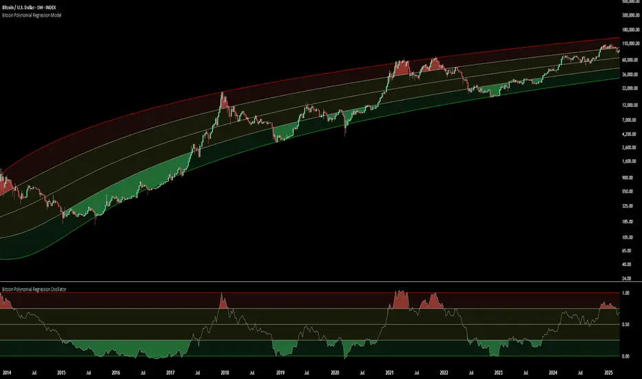
Bitcoin Polynomial Regression ModelThis is the main version of the script. Click here for the Oscillator part of the script.
💡Why this model was created:
One of the key issues with most existing models, including our own Bitcoin Log Growth Curve Model , is that they often fail to realistically account for diminishing returns. As a result, they may present overly optimistic bull cycle targets (hence, we introduced alternative settings in our previous Bitcoin Log Growth Curve Model).
This new model however, has been built from the ground up with a primary focus on incorporating the principle of diminishing returns. It directly responds to this concept, which has been briefly explored here .
📉The theory of diminishing returns:
This theory suggests that as each four-year market cycle unfolds, volatility gradually decreases, leading to more tempered price movements. It also implies that the price increase from one cycle peak to the next will decrease over time as the asset matures. The same pattern applies to cycle lows and the relationship between tops and bottoms. In essence, these price movements are interconnected and should generally follow a consistent pattern. We believe this model provides a more realistic outlook on bull and bear market cycles.
To better understand this theory, the relationships between cycle tops and bottoms are outlined below:https://www.tradingview.com/x/7Hldzsf2/
🔧Creation of the model:
For those interested in how this model was created, the process is explained here. Otherwise, feel free to skip this section.
This model is based on two separate cubic polynomial regression lines. One for the top price trend and another for the bottom. Both follow the general cubic polynomial function:
ax^3 +bx^2 + cx + d.
In this equation, x represents the weekly bar index minus an offset, while a, b, c, and d are determined through polynomial regression analysis. The input (x, y) values used for the polynomial regression analysis are as follows:
Top regression line (x, y) values:
113, 18.6
240, 1004
451, 19128
655, 65502
Bottom regression line (x, y) values:
103, 2.5
267, 211
471, 3193
676, 16255
The values above correspond to historical Bitcoin cycle tops and bottoms, where x is the weekly bar index and y is the weekly closing price of Bitcoin. The best fit is determined using metrics such as R-squared values, residual error analysis, and visual inspection. While the exact details of this evaluation are beyond the scope of this post, the following optimal parameters were found:
Top regression line parameter values:
a: 0.000202798
b: 0.0872922
c: -30.88805
d: 1827.14113
Bottom regression line parameter values:
a: 0.000138314
b: -0.0768236
c: 13.90555
d: -765.8892
📊Polynomial Regression Oscillator:
This publication also includes the oscillator version of the this model which is displayed at the bottom of the screen. The oscillator applies a logarithmic transformation to the price and the regression lines using the formula log10(x) .
The log-transformed price is then normalized using min-max normalization relative to the log-transformed top and bottom regression line with the formula:
normalized price = log(close) - log(bottom regression line) / log(top regression line) - log(bottom regression line)
This transformation results in a price value between 0 and 1 between both the regression lines. The Oscillator version can be found here.
🔍Interpretation of the Model:
In general, the red area represents a caution zone, as historically, the price has often been near its cycle market top within this range. On the other hand, the green area is considered an area of opportunity, as historically, it has corresponded to the market bottom.
The top regression line serves as a signal for the absolute market cycle peak, while the bottom regression line indicates the absolute market cycle bottom.
Additionally, this model provides a predicted range for Bitcoin's future price movements, which can be used to make extrapolated predictions. We will explore this further below.
🔮Future Predictions:
Finally, let's discuss what this model actually predicts for the potential upcoming market cycle top and the corresponding market cycle bottom. In our previous post here , a cycle interval analysis was performed to predict a likely time window for the next cycle top and bottom:
In the image, it is predicted that the next top-to-top cycle interval will be 208 weeks, which translates to November 3rd, 2025. It is also predicted that the bottom-to-top cycle interval will be 152 weeks, which corresponds to October 13th, 2025. On the macro level, these two dates align quite well. For our prediction, we take the average of these two dates: October 24th 2025. This will be our target date for the bull cycle top.
Now, let's do the same for the upcoming cycle bottom. The bottom-to-bottom cycle interval is predicted to be 205 weeks, which translates to October 19th, 2026, and the top-to-bottom cycle interval is predicted to be 259 weeks, which corresponds to October 26th, 2026. We then take the average of these two dates, predicting a bear cycle bottom date target of October 19th, 2026.
Now that we have our predicted top and bottom cycle date targets, we can simply reference these two dates to our model, giving us the Bitcoin top price prediction in the range of 152,000 in Q4 2025 and a subsequent bottom price prediction in the range of 46,500 in Q4 2026.
For those interested in understanding what this specifically means for the predicted diminishing return top and bottom cycle values, the image below displays these predicted values. The new values are highlighted in yellow:
And of course, keep in mind that these targets are just rough estimates. While we've done our best to estimate these targets through a data-driven approach, markets will always remain unpredictable in nature. What are your targets? Feel free to share them in the comment section below.

Bitcoin Polynomial Regression OscillatorThis is the oscillator version of the script. Click here for the other part of the script.
💡Why this model was created:
One of the key issues with most existing models, including our own Bitcoin Log Growth Curve Model , is that they often fail to realistically account for diminishing returns. As a result, they may present overly optimistic bull cycle targets (hence, we introduced alternative settings in our previous Bitcoin Log Growth Curve Model).
This new model however, has been built from the ground up with a primary focus on incorporating the principle of diminishing returns. It directly responds to this concept, which has been briefly explored here .
📉The theory of diminishing returns:
This theory suggests that as each four-year market cycle unfolds, volatility gradually decreases, leading to more tempered price movements. It also implies that the price increase from one cycle peak to the next will decrease over time as the asset matures. The same pattern applies to cycle lows and the relationship between tops and bottoms. In essence, these price movements are interconnected and should generally follow a consistent pattern. We believe this model provides a more realistic outlook on bull and bear market cycles.
To better understand this theory, the relationships between cycle tops and bottoms are outlined below:https://www.tradingview.com/x/7Hldzsf2/
🔧Creation of the model:
For those interested in how this model was created, the process is explained here. Otherwise, feel free to skip this section.
This model is based on two separate cubic polynomial regression lines. One for the top price trend and another for the bottom. Both follow the general cubic polynomial function:
ax^3 +bx^2 + cx + d.
In this equation, x represents the weekly bar index minus an offset, while a, b, c, and d are determined through polynomial regression analysis. The input (x, y) values used for the polynomial regression analysis are as follows:
Top regression line (x, y) values:
113, 18.6
240, 1004
451, 19128
655, 65502
Bottom regression line (x, y) values:
103, 2.5
267, 211
471, 3193
676, 16255
The values above correspond to historical Bitcoin cycle tops and bottoms, where x is the weekly bar index and y is the weekly closing price of Bitcoin. The best fit is determined using metrics such as R-squared values, residual error analysis, and visual inspection. While the exact details of this evaluation are beyond the scope of this post, the following optimal parameters were found:
Top regression line parameter values:
a: 0.000202798
b: 0.0872922
c: -30.88805
d: 1827.14113
Bottom regression line parameter values:
a: 0.000138314
b: -0.0768236
c: 13.90555
d: -765.8892
📊Polynomial Regression Oscillator:
This publication also includes the oscillator version of the this model which is displayed at the bottom of the screen. The oscillator applies a logarithmic transformation to the price and the regression lines using the formula log10(x) .
The log-transformed price is then normalized using min-max normalization relative to the log-transformed top and bottom regression line with the formula:
normalized price = log(close) - log(bottom regression line) / log(top regression line) - log(bottom regression line)
This transformation results in a price value between 0 and 1 between both the regression lines.
🔍Interpretation of the Model:
In general, the red area represents a caution zone, as historically, the price has often been near its cycle market top within this range. On the other hand, the green area is considered an area of opportunity, as historically, it has corresponded to the market bottom.
The top regression line serves as a signal for the absolute market cycle peak, while the bottom regression line indicates the absolute market cycle bottom.
Additionally, this model provides a predicted range for Bitcoin's future price movements, which can be used to make extrapolated predictions. We will explore this further below.
🔮Future Predictions:
Finally, let's discuss what this model actually predicts for the potential upcoming market cycle top and the corresponding market cycle bottom. In our previous post here , a cycle interval analysis was performed to predict a likely time window for the next cycle top and bottom:
In the image, it is predicted that the next top-to-top cycle interval will be 208 weeks, which translates to November 3rd, 2025. It is also predicted that the bottom-to-top cycle interval will be 152 weeks, which corresponds to October 13th, 2025. On the macro level, these two dates align quite well. For our prediction, we take the average of these two dates: October 24th 2025. This will be our target date for the bull cycle top.
Now, let's do the same for the upcoming cycle bottom. The bottom-to-bottom cycle interval is predicted to be 205 weeks, which translates to October 19th, 2026, and the top-to-bottom cycle interval is predicted to be 259 weeks, which corresponds to October 26th, 2026. We then take the average of these two dates, predicting a bear cycle bottom date target of October 19th, 2026.
Now that we have our predicted top and bottom cycle date targets, we can simply reference these two dates to our model, giving us the Bitcoin top price prediction in the range of 152,000 in Q4 2025 and a subsequent bottom price prediction in the range of 46,500 in Q4 2026.
For those interested in understanding what this specifically means for the predicted diminishing return top and bottom cycle values, the image below displays these predicted values. The new values are highlighted in yellow:
And of course, keep in mind that these targets are just rough estimates. While we've done our best to estimate these targets through a data-driven approach, markets will always remain unpredictable in nature. What are your targets? Feel free to share them in the comment section below.
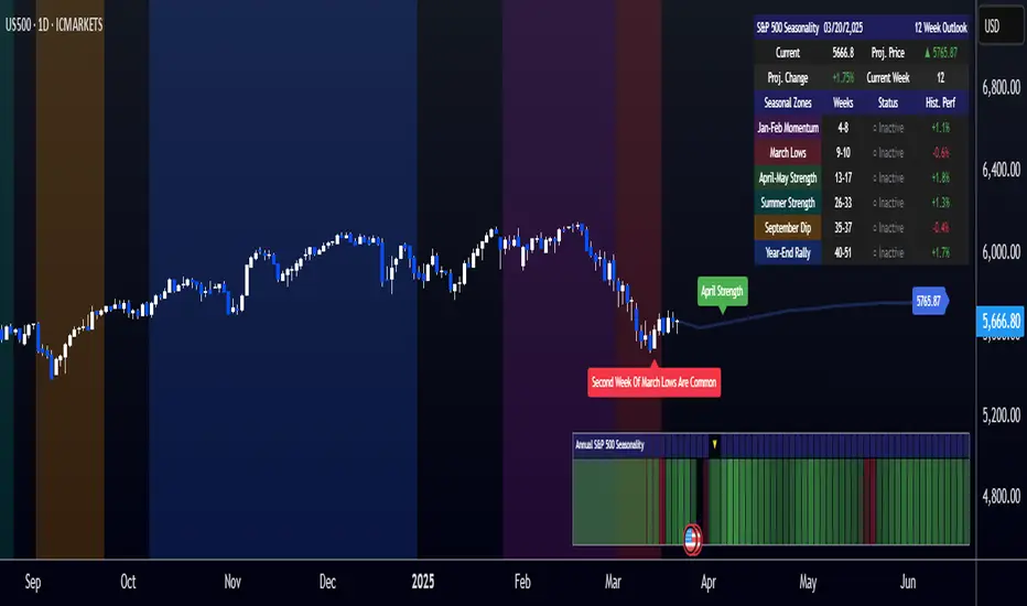
[COG]S&P 500 Weekly Seasonality ProjectionS&P 500 Weekly Seasonality Projection
This indicator visualizes S&P 500 seasonality patterns based on historical weekly performance data. It projects price movements for up to 26 weeks ahead, highlighting key seasonal periods that have historically affected market performance.
Key Features:
Projects price movements based on historical S&P 500 weekly seasonality patterns (2005-2024)
Highlights six key seasonal periods: Jan-Feb Momentum, March Lows, April-May Strength, Summer Strength, September Dip, and Year-End Rally
Customizable forecast length from 1-26 weeks with quick timeframe selection buttons
Optional moving average smoothing for more gradual projections
Detailed statistics table showing projected price and percentage change
Seasonality mini-map showing the full annual pattern with current position
Customizable colors and visual elements
How to Use:
Apply to S&P 500 index or related instruments (daily timeframe or higher recommended)
Set your desired forecast length (1-26 weeks)
Monitor highlighted seasonal zones that have historically shown consistent patterns
Use the projection line as a general guideline for potential price movement
Settings:
Forecast length: Configure from 1-26 weeks or use quick select buttons (1M, 3M, 6M, 1Y)
Visual options: Customize colors, backgrounds, label sizes, and table position
Display options: Toggle statistics table, period highlights, labels, and mini-map
This indicator is designed as a visual guide to help identify potential seasonal tendencies in the S&P 500. Historical patterns are not guarantees of future performance, but understanding these seasonal biases can provide valuable context for your trading decisions.
Note: For optimal visualization, use on Daily timeframe or higher. Intraday timeframes will display a warning message.
Bitcoin Halving DatesBitcoin Halving Dates Indicator
This custom indicator automatically marks Bitcoin's key halving events by drawing vertical lines on your chart. It highlights the historical halving dates (2012, 2016, 2020) and includes an estimated date for the upcoming halving in 2024, making it easy to visualize significant supply events that can influence market trends.
Features:
Automated Markings: Displays vertical lines on the first bar of each halving day.
Customizable: Easily adjust halving dates and styling options to suit your analysis.
Built for Traders: Enhance your technical analysis by keeping track of pivotal market events.
Use this indicator to gain a visual edge by integrating critical Bitcoin halving events into your trading strategy. Happy Trading!

MM Labelled AVWAPTradingView provides a tool to show anchored VWAP plots on your screen, but there is no way to label the plots to add additional context to the level. Instead, users are forced to use the plot style (color, line style, line thickness, etc) to indicate what the plots are for and then they have to remember that meaning when looking at different charts. It also means that for key market-wide moments, users will need to add the plot for every symbol.
Now, for the first time on TradingView, you can create anchored VWAP plots with labels on them so you can understand the meaning behind the key moments you care about and don't need to remember what they mean by using styles like color or thickness. You can use this indicator to track key moments like the 2022 market bottom, or the Aug 9, 2024 "Carry Trade Unwind" bottom. The labelled AVWAP plots are visible on every chart by default. If you have an AVWAP moment that is only relevant to a small number of symbols, you can configure the indicator to only appear on those symbols.

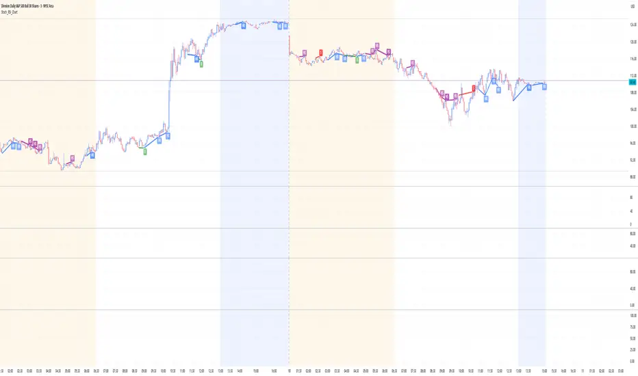
TEMA OBOS Strategy PakunTEMA OBOS Strategy
Overview
This strategy combines a trend-following approach using the Triple Exponential Moving Average (TEMA) with Overbought/Oversold (OBOS) indicator filtering.
By utilizing TEMA crossovers to determine trend direction and OBOS as a filter, it aims to improve entry precision.
This strategy can be applied to markets such as Forex, Stocks, and Crypto, and is particularly designed for mid-term timeframes (5-minute to 1-hour charts).
Strategy Objectives
Identify trend direction using TEMA
Use OBOS to filter out overbought/oversold conditions
Implement ATR-based dynamic risk management
Key Features
1. Trend Analysis Using TEMA
Uses crossover of short-term EMA (ema3) and long-term EMA (ema4) to determine entries.
ema4 acts as the primary trend filter.
2. Overbought/Oversold (OBOS) Filtering
Long Entry Condition: up > down (bullish trend confirmed)
Short Entry Condition: up < down (bearish trend confirmed)
Reduces unnecessary trades by filtering extreme market conditions.
3. ATR-Based Take Profit (TP) & Stop Loss (SL)
Adjustable ATR multiplier for TP/SL
Default settings:
TP = ATR × 5
SL = ATR × 2
Fully customizable risk parameters.
4. Customizable Parameters
TEMA Length (for trend calculation)
OBOS Length (for overbought/oversold detection)
Take Profit Multiplier
Stop Loss Multiplier
EMA Display (Enable/Disable TEMA lines)
Bar Color Change (Enable/Disable candle coloring)
Trading Rules
Long Entry (Buy Entry)
ema3 crosses above ema4 (Golden Cross)
OBOS indicator confirms up > down (bullish trend)
Execute a buy position
Short Entry (Sell Entry)
ema3 crosses below ema4 (Death Cross)
OBOS indicator confirms up < down (bearish trend)
Execute a sell position
Take Profit (TP)
Entry Price + (ATR × TP Multiplier) (Default: 5)
Stop Loss (SL)
Entry Price - (ATR × SL Multiplier) (Default: 2)
TP/SL settings are fully customizable to fine-tune risk management.
Risk Management Parameters
This strategy emphasizes proper position sizing and risk control to balance risk and return.
Trading Parameters & Considerations
Initial Account Balance: $7,000 (adjustable)
Base Currency: USD
Order Size: 10,000 USD
Pyramiding: 1
Trading Fees: $0.94 per trade
Long Position Margin: 50%
Short Position Margin: 50%
Total Trades (M5 Timeframe): 128
Deep Test Results (2024/11/01 - 2025/02/24)BTCUSD-5M
Total P&L:+1638.20USD
Max equity drawdown:694.78USD
Total trades:128
Profitable trades:44.53
Profit factor:1.45
These settings aim to protect capital while maintaining a balanced risk-reward approach.
Visual Support
TEMA Lines (Three EMAs)
Trend direction is indicated by color changes (Blue/Orange)
ema3 (short-term) and ema4 (long-term) crossover signals potential entries
OBOS Histogram
Green → Strong buying pressure
Red → Strong selling pressure
Blue → Possible trend reversal
Entry & Exit Markers
Blue Arrow → Long Entry Signal
Red Arrow → Short Entry Signal
Take Profit / Stop Loss levels displayed
Strategy Improvements & Uniqueness
This strategy is based on indicators developed by "l_lonthoff" and "jdmonto0", but has been significantly optimized for better entry accuracy, visual clarity, and risk management.
Enhanced Trend Identification with TEMA
Detects early trend reversals using ema3 & ema4 crossover
Reduces market noise for a smoother trend-following approach
Improved OBOS Filtering
Prevents excessive trading
Reduces unnecessary risk exposure
Dynamic Risk Management with ATR-Based TP/SL
Not a fixed value → TP/SL adjusts to market volatility
Fully customizable ATR multiplier settings
(Default: TP = ATR × 5, SL = ATR × 2)
Summary
The TEMA + OBOS Strategy is a simple yet powerful trading method that integrates trend analysis and oscillators.
TEMA for trend identification
OBOS for noise reduction & overbought/oversold filtering
ATR-based TP/SL settings for dynamic risk management
Before using this strategy, ensure thorough backtesting and demo trading to fine-tune parameters according to your trading style.

[GYTS] FiltersToolkit LibraryFiltersToolkit Library
🌸 Part of GoemonYae Trading System (GYTS) 🌸
🌸 --------- 1. INTRODUCTION --------- 🌸
💮 What Does This Library Contain?
This library is a curated collection of high-performance digital signal processing (DSP) filters and auxiliary functions designed specifically for financial time series analysis. It includes a shortlist of our favourite and best performing filters — each rigorously tested and selected for their responsiveness, minimal lag and robustness in diverse market conditions. These tools form an integral part of the GoemonYae Trading System (GYTS), chosen for their unique characteristics in handling market data.
The library contains two main categories:
1. Smoothing filters (low-pass filters and moving averages) for e.g. denoising, trend following
2. Detrending tools (high-pass and band-pass filters, known as "oscillators") for e.g. mean reversion
This collection is finely tuned for practical trading applications and is therefore not meant to be exhaustive. However, will continue to expand as we discover and validate new filtering techniques. I welcome collaboration and suggestions for novel approaches.
🌸 ——— 2. ADDED VALUE ——— 🌸
💮 Unified syntax and comprehensive documentation
The FiltersToolkit Library brings together a wide array of valuable filters under a unified, intuitive syntax. Each function is thoroughly documented, with clear explanations and academic sources that underline the mathematical rigour behind the methods. This level of documentation not only facilitates integration into trading strategies but also helps underlying the underlying concepts and rationale.
💮 Optimised performance and readability
The code prioritizes computational efficiency while maintaining readability. Key optimizations include:
- Minimizing redundant calculations in recursive filters
- Smart coefficient caching
- Efficient state management
- Vectorized operations where applicable
💮 Enhanced functionality and flexibility
Some filters in this library introduce extended functionality beyond the original publications. For instance, the MESA Adaptive Moving Average (MAMA) and Ehlers’ Combined Bandpass Filter incorporate multiple variations found in the literature, thereby providing traders with flexible tools that can be fine-tuned to different market conditions.
🌸 ——— 3. THE FILTERS ——— 🌸
💮 Hilbert Transform Function
This function implements the Hilbert Transform as utilised by John Ehlers. It converts a real-valued time series into its analytic signal, enabling the extraction of instantaneous phase and frequency information—an essential step in adaptive filtering.
Source: John Ehlers - "Rocket Science for Traders" (2001), "TASC 2001 V. 19:9", "Cybernetic Analysis for Stocks and Futures" (2004)
💮 Homodyne Discriminator
By leveraging the Hilbert Transform, this function computes the dominant cycle period through a Homodyne Discriminator. It extracts the in-phase and quadrature components of the signal, facilitating a robust estimation of the underlying cycle characteristics.
Source: John Ehlers - "Rocket Science for Traders" (2001), "TASC 2001 V. 19:9", "Cybernetic Analysis for Stocks and Futures" (2004)
💮 MESA Adaptive Moving Average (MAMA)
An advanced dual-stage adaptive moving average, this function outputs both the MAMA and its companion FAMA. It combines adaptive alpha computation with elements from Kaufman’s Adaptive Moving Average (KAMA) to provide a responsive and reliable trend indicator.
Source: John Ehlers - "Rocket Science for Traders" (2001), "TASC 2001 V. 19:9", "Cybernetic Analysis for Stocks and Futures" (2004)
💮 BiQuad Filters
A family of second-order recursive filters offering exceptional control over frequency response:
- High-pass filter for detrending
- Low-pass filter for smooth trend following
- Band-pass filter for cycle isolation
The quality factor (Q) parameter allows fine-tuning of the resonance characteristics, making these filters highly adaptable to different market conditions.
Source: Robert Bristow-Johnson's Audio EQ Cookbook, implemented by @The_Peaceful_Lizard
💮 Relative Vigor Index (RVI)
This filter evaluates the strength of a trend by comparing the closing price to the trading range. Operating similarly to a band-pass filter, the RVI provides insights into market momentum and potential reversals.
Source: John Ehlers – “Cybernetic Analysis for Stocks and Futures” (2004)
💮 Cyber Cycle
The Cyber Cycle filter emphasises market cycles by smoothing out noise and highlighting the dominant cyclical behaviour. It is particularly useful for detecting trend reversals and cyclical patterns in the price data.
Source: John Ehlers – “Cybernetic Analysis for Stocks and Futures” (2004)
💮 Butterworth High Pass Filter
Inspired by the classical Butterworth design, this filter achieves a maximally flat magnitude response in the passband while effectively removing low-frequency trends. Its design minimises phase distortion, which is vital for accurate signal interpretation.
Source: John Ehlers – “Cybernetic Analysis for Stocks and Futures” (2004)
💮 2-Pole SuperSmoother
Employing a two-pole design, the SuperSmoother filter reduces high-frequency noise with minimal lag. It is engineered to preserve trend integrity while offering a smooth output even in noisy market conditions.
Source: John Ehlers – “Cybernetic Analysis for Stocks and Futures” (2004)
💮 3-Pole SuperSmoother
An extension of the 2-pole design, the 3-pole SuperSmoother further attenuates high-frequency noise. Its additional pole delivers enhanced smoothing at the cost of slightly increased lag.
Source: John Ehlers – “Cybernetic Analysis for Stocks and Futures” (2004)
💮 Adaptive Directional Volatility Moving Average (ADXVma)
This adaptive moving average adjusts its smoothing factor based on directional volatility. By combining true range and directional movement measurements, it remains exceptionally flat during ranging markets and responsive during directional moves.
Source: Various implementations across platforms, unified and optimized
💮 Ehlers Combined Bandpass Filter with Automated Gain Control (AGC)
This sophisticated filter merges a highpass pre-processing stage with a bandpass filter. An integrated Automated Gain Control normalises the output to a consistent range, while offering both regular and truncated recursive formulations to manage lag.
Source: John F. Ehlers – “Truncated Indicators” (2020), “Cycle Analytics for Traders” (2013)
💮 Voss Predictive Filter
A forward-looking filter that predicts future values of a band-limited signal in real time. By utilising multiple time-delayed feedback terms, it provides anticipatory coupling and delivers a short-term predictive signal.
Source: John Ehlers - "A Peek Into The Future" (TASC 2019-08)
💮 Adaptive Autonomous Recursive Moving Average (A2RMA)
This filter dynamically adjusts its smoothing through an adaptive mechanism based on an efficiency ratio and a dynamic threshold. A double application of an adaptive moving average ensures both responsiveness and stability in volatile and ranging markets alike. Very flat response when properly tuned.
Source: @alexgrover (2019)
💮 Ultimate Smoother (2-Pole)
The Ultimate Smoother filter is engineered to achieve near-zero lag in its passband by subtracting a high-pass response from an all-pass response. This creates a filter that maintains signal fidelity at low frequencies while effectively filtering higher frequencies at the expense of slight overshooting.
Source: John Ehlers - TASC 2024-04 "The Ultimate Smoother"
Note: This library is actively maintained and enhanced. Suggestions for additional filters or improvements are welcome through the usual channels. The source code contains a list of tested filters that did not make it into the curated collection.
Best Buffett Ratio w/ Std-Dev Offset + Conditional PlotSummary:
This script provides a visually clear way to track the so-called “Buffett Ratio,”
a popular market valuation gauge which compares the total US stock market cap
to the country’s GDP. In addition, it plots a “hardcoded” long-term trend line,
along with fixed standard-deviation bands (in log space), and uses background colors
to signal potentially overvalued or undervalued zones.
What Is the Buffett Ratio?
Often credited to Warren Buffett, the Buffett Ratio (or Buffett Indicator) measures:
(Total US Stock Market Capitalization) / (US GDP)
• A higher ratio typically means equities are more expensive relative to the size of the economy.
• A lower ratio suggests equities may be more attractively valued compared to GDP.
Historically, the ratio has tended to drift upward over many decades,
as the US economy and stock markets grow, but it still oscillates around some trend over time.
How to Use
1) Add to Chart:
- In TradingView, simply apply the indicator (it internally fetches CRSPTM1 & GDP data).
2) Tweak Inputs:
- Log Offset for 1σ: Adjust how wide the ±1σ/±2σ bands appear around the trend.
- Anchor Points: Edit startYear , endYear , startRatio , endRatio
if you want a different slope or different “fair value” anchors.
3) Interpretation:
- If the indicator is above +2σ (red line) , it’s historically “very expensive,”
often leading to lower future returns over the long term.
- If it’s below –2σ (green line) , it’s historically “deep undervaluation,”
often pointing to better future returns over time.
- The intermediate zones show degrees of mild over- or undervaluation.
How This Script Works
1) Buffett Ratio Calculation:
- The script requests data from TradingView’s built-in CRSPTM1 index (total US market cap).
- It also requests US GDP data via request.economic("US", "GDP") .
- If GDP data is missing, the ratio becomes na on that bar.
2) Hardcoded Trend Line:
- Rather than a rolling average, the script uses two “anchors” (e.g. 1950 → 0.30 ratio, 2024 → 1.25 ratio)
and solves for a single log-growth rate to produce a steady upward slope.
3) Fixed Standard Deviations in Log Space:
- The script takes the log of the trend line, then applies a fixed offset for ±1σ and ±2σ,
creating proportional bands that do not “expand/contract” from a rolling window.
4) Conditional Plotting:
- The script only begins plotting once the Buffett Ratio actually has data (around 2011).
5) Color-Coded Zones:
- Above +2σ: red background (historically very expensive)
- Between +1σ and +2σ: yellow background (moderately expensive)
- Between –1σ and +1σ: no background color (around normal)
- Between –2σ and –1σ: aqua background (moderately undervalued)
- Below –2σ: green background (historically deep undervaluation)
Final Notes
• Data Limitations: US GDP data and CRSPTM1 only go back so far, so this starts around 2011.
• Long-Term vs. Short-Term: Best viewed on monthly/quarterly charts and interpreted over years.
• Tuning: If you believe structural changes have shifted the ratio’s fair slope,
adjust the code’s anchors or log offsets.
Enjoy, and use responsibly!

Ehlers Maclaurin Ultimate Smoother [CT]Ehlers Maclaurin Ultimate Smoother
Introduction
The Ehlers Maclaurin Ultimate Smoother is an innovative enhancement of the classic Ehlers SuperSmoother. By leveraging advanced Maclaurin series approximations, this indicator offers superior market analysis and signal generation.
The indicator combines Ehlers' Ultimate Smoother with Maclaurin series approximations to create a more efficient and accurate smoothing mechanism:
Input price data passes through the initial smoothing phase
Maclaurin series approximates trigonometric functions
Enhanced high-pass filter removes market noise
Final smoothing phase produces the output signal
Why the Maclaurin Approach?
The Maclaurin series is a special form of the Taylor series, centered around 0. It provides an efficient way to approximate complex functions using polynomial terms. In this indicator, we use the Maclaurin approach to improve the sine and cosine functions, resulting in:
Faster Calculations: By using polynomial approximations, we significantly reduce computational complexity.
Improved Stability: The approximation provides a more stable numerical basis for calculations.
Preservation of Precision: Despite the approximation, we maintain the precision needed for price smoothing.
Calculations
The indicator employs several key mathematical components:
Maclaurin Series Approximation:
sin(x) ≈ x - x³/3! + x⁵/5! - x⁷/7! + x⁹/9!
cos(x) ≈ 1 - x²/2! + x⁴/4! - x⁶/6! + x⁸/8!
Smoothing Algorithm:
Uses exponential smoothing with optimized coefficients
Implements high-pass filtering for noise reduction
Applies dynamic weighting based on market conditions
Mathematical Foundation
Utilizes Maclaurin series for trigonometric approximation
Implements Ehlers' smoothing principles
Incorporates advanced filtering techniques
Technical Advantages
Signal Processing:
Lag Reduction: Faster signal detection with less delay.
Noise Filtration: Effective elimination of high-frequency noise.
Precision Enhancement: Preservation of critical price movements.
Adaptive Processing: Dynamic response to market volatility.
Visual Enhancements:
Smart color intensity mapping.
Real-time visualization of trend strength.
Adaptive opacity based on movement significance.
Implementation
Core Configuration:
Plot Type: Choose between the original and the Maclaurin enhanced version.
Length: Default set to 30, optimal for daily timeframes.
hpLength: Default set to 10 for enhanced noise reduction.
Advanced Parameters:
The indicator offers advanced control with:
Dual processing modes (Original/Maclaurin).
Dynamic color intensity system.
Customizable smoothing parameters.
Professional Analysis Tools:
Accurate trend reversal identification.
Advanced support/resistance detection.
Superior performance in volatile markets.
Technical Specifications
Maclaurin Series Implementation:
The indicator employs a 5-term Maclaurin series approximation for both sine and cosine, ensuring efficient and accurate computation.
Performance Metrics
Improved processing efficiency.
Reduced memory utilization.
Increased signal accuracy.
Licensing & Attribution
© 2024 Mupsje aka CasaTropical
Professional Credits
Original Ultimate and SuperSmoother concept: John F. Ehlers
Maclaurin enhancement: Casa Tropical (CT)
www.mathsisfun.com

SW monthly Gann Days**Script Description:**
The script you are looking at is based on the work of W.D. Gann, a famous trader and market analyst in the early 20th century, known for his use of geometry, astrology, and numerology in market analysis. Gann believed that certain days in the market had significant importance, and he observed that markets often exhibited significant price moves around specific dates. These dates were typically associated with cyclical patterns in price movements, and Gann referred to these as "Gann Days."
In this script, we have focused on highlighting certain days of the month that Gann believed to have an influence on market behavior. The specific days in question are the **6th to 7th**, **9th to 10th**, **14th to 15th**, **19th to 20th**, **23rd to 24th**, and **29th to 31st** of each month. These ranges are based on Gann’s theory that there are recurring time cycles in the market that cause turning points or critical price movements to occur around certain days of the month.
### **Why Gann Used These Days:**
1. **Mathematical and Astrological Cycles:**
Gann believed that markets were influenced by natural cycles, and that certain dates (or combinations of dates) played a critical role in the price movements. These specific days are part of his broader theory of "time cycles" where the market would often change direction, reverse, or exhibit significant volatility on particular days. Gann's research was based on both mathematical principles and astrological observations, leading him to assign importance to these days.
2. **Gann's Universal Timing Theory:**
According to Gann, financial markets operate in a universe governed by geometric and astrological principles. These cycles repeat themselves over time, and specific days in a given month correspond to key turning points within these repeating cycles. Gann found that the 6th to 7th, 9th to 10th, 14th to 15th, 19th to 20th, 23rd to 24th, and 29th to 31st often marked significant changes in the market, making them particularly important for traders to watch.
3. **Market Psychology and Sentiment:**
These specific days likely correspond to key moments where market participants tend to react in predictable ways, influenced by past market behavior on similar dates. For example, news events or scheduled economic reports might fall within these time windows, causing the market to respond in a particular way. Gann's method involves using these cyclical patterns to predict turning points in market prices, enabling traders to anticipate when the market might make a reversal or face a significant shift in direction.
4. **Turning Points:**
Gann believed that markets often reversed or encountered critical points around specific dates. This is why he considered certain days more important than others. By identifying and focusing on these days, traders can better anticipate the market’s movement and make more informed trading decisions.
5. **Numerology:**
Gann also utilized numerology in his trading system, believing that numbers, and particularly certain key numbers, had significance in predicting market movements. The days selected in this script may correspond to numerological patterns that Gann identified in his analysis of the markets, such as recurring numbers in his astrological and geometric systems.
### **Purpose of the Script:**
This script highlights these "Gann Days" within a trading chart for 2024 and 2025. The color-coding or background highlighting is intended to draw attention to these dates, so traders can observe the potential for significant market movements during these times. By identifying these specific dates, traders following Gann's theories may gain insights into possible turning points, corrections, or key price movements based on the market's historical behavior around these days.
Overall, Gann’s use of specific days was based on his deep belief in the cyclical nature of the market and his attempt to tie those cycles to the natural laws of time, geometry, and astrology. By focusing on these dates, Gann aimed to give traders an edge in predicting significant market events and price shifts.
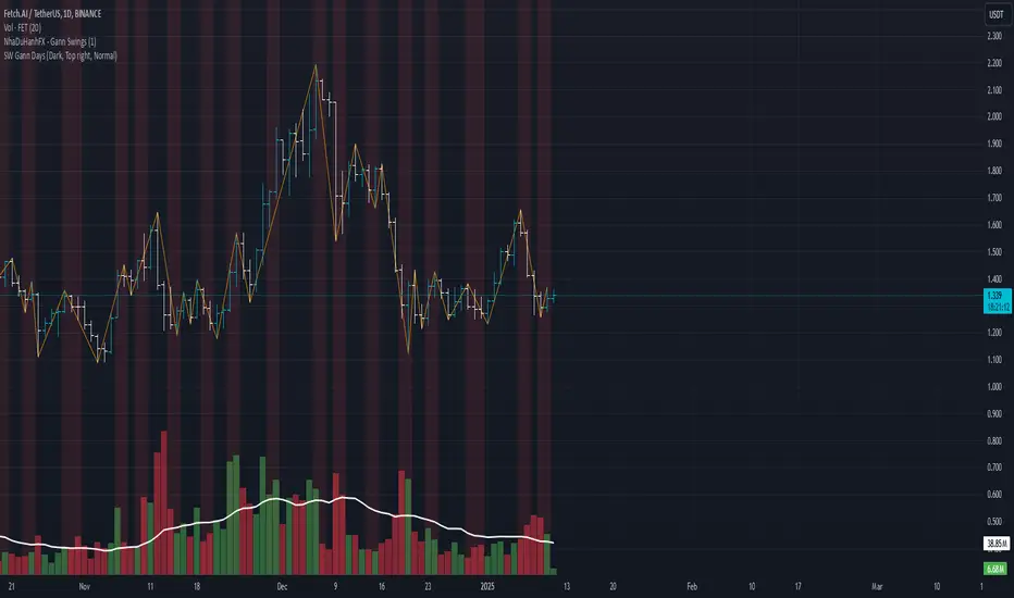
Follow Through Day (FTD) + Sweep [TrendX_]The Follow Through Day (FTD) + Sweep indicator is a Trend-following tool mixing William O'Neil's original FTD concept and Liquidity concept. This indicator helps you identify potential subsequent bullish trends with greater precision by combining volume analysis, price action, and liquidity concepts.
💎 FEATURES
Follow Through Day Candle (FTD Candle)
The FTD, pioneered by William O'Neil, serves as a reliable signal for identifying the beginning of new bull markets. It's particularly valuable because it combines multiple market factors - price action, volume, and timing - to confirm genuine market reversals rather than temporary bounces.
The power of the FTD lies in its ability to distinguish between ordinary market fluctuations and significant trend changes. By requiring specific criteria to be met across multiple sessions, it helps filter out false signals and identifies high-probability reversal points where institutional investors are likely beginning to accumulate positions.
Sweep Area
The Sweep area feature enhances the traditional FTD concept by incorporating modern liquidity analysis. This overlay identifies zones where large market participants are likely to trigger stop losses before continuing the trend. These areas often represent optimal entry points for traders looking to join the new uptrend with reduced risk.
🔎 BREAKDOWN
FTD Candle
The FTD formation process occurs in two distinct phases: Setup and Completion.
Setup Phase
Strong Market Decline
The market must first experience a significant downtrend
This selling pressure helps clear out weak hands and creates oversold conditions
The decline creates the potential energy for a powerful reversal
First Recovery Session
Marks the initial sign of buying pressure emerging
Often characterized by a strong reversal candle
Represents the first indication that selling pressure may be exhausting
Recovery Confirmation
The second and third days must maintain prices above the new pivot low
This consolidation period helps confirm the validity of the initial bounce
Shows that sellers are no longer in control of price action
Completion Phase:
Supply Test Session
Low volume indicates diminishing selling pressure
Price remains above the pivot low
Creates the foundation for institutional buyers to begin accumulating
Breakout Day
Price increase exceeds average profit of bullish candles
Volume increases by at least 15% compared to previous session
Shows strong institutional commitment to the new uptrend
Timing Window
Must occur between the 4th and 8th candle after First Recovery Session
This specific timing helps confirm the sustainability of the reversal
Based on O'Neil's research of historical market bottoms
FTD Sweep
The Post-FTD Phase introduces the Sweep concept, which is crucial for understanding how large market participants operate. This feature leverages the liquidity concept because institutional traders often need to trigger stop losses to accumulate larger positions at better prices. This helps:
Create liquidity pools for large position entries
Shake out weak hands before continuing the trend
Test the strength of the new trend by absorbing selling pressure
⚙️ USAGE
Sweep + TP & SL Strategy
Example: BTCUSDT (1D) - Replay back to 9th November 2024
After an FTD candle forms, traders can adopt a systematic approach to enhance their trading strategy. First, they should determine the swing range and convert the post-FTD zone into concrete stop loss and take profit levels, which are based on the price action during the FTD formation. Next, traders should wait for a sweep formation, as this indicates that institutional players are accumulating positions. A quick price rejection from the sweep level should be observed before executing an entry.
The reasoning behind this strategy is rooted in market microstructure. By waiting for the sweep, traders position themselves alongside institutional players who need to build large positions without causing adverse price movement. The sweep creates the liquidity they need, and the subsequent move often represents the true trend continuation.
DISCLAIMER
This indicator is not financial advice, it can only help traders make better decisions. There are many factors and uncertainties that can affect the outcome of any endeavor, and no one can guarantee or predict with certainty what will occur. Therefore, one should always exercise caution and judgment when making decisions based on past performance.
