DBG X WOLONG📊 USER GUIDE – DBG X WOLONG ALGORITHM
🎯 OVERVIEW
The DBG X WOLONG Future Algorithm is a Pine Script v5 that integrates multiple advanced technical indicators, enabling traders to analyze markets and make precise trading decisions.
⚙️ MAIN SETTINGS
🔹 Sensitivity
Value: 1–20 (Default: 6)
Function: Adjusts the sensitivity of the SuperTrend signal
Guidelines:
Low value (1–5): Fewer signals, higher accuracy
High value (15–20): More signals, but with possible noise
🎨 DISPLAY SETTINGS
🔹 Candle Colors
Version 1: Based on MACD histogram
Version 2: Based on SuperTrend
🔹 Color Themes
Theme 1: Traditional Green/Red
Theme 2: Gold/Purple
Theme 3: Blue/Orange
No Fill: No background color displayed
📊 TRADING SIGNALS
🔹 Buy/Sell Signals
BUY 🚀 appears when:
SuperTrend shifts from bearish to bullish
Closing price > SMA 13
Braid Filter confirms
SELL appears when:
SuperTrend shifts from bullish to bearish
Closing price < SMA 13
Braid Filter confirms
🔹 Reversal Signals
▲ (Up Arrow): Buy signal when RSI crosses above 30
▼ (Down Arrow): Sell signal when RSI crosses below 70
🔹 Pullback Signals
▲ Purple: Pullback in bullish trend
▼ Purple: Pullback in bearish trend
🎯 TAKE PROFIT & STOP LOSS
🔹 TP Modes
Version 1: TP based on pivot points
Version 2: TP based on regression line
Close Price: TP at candle close
🔹 TP/SL Settings
TP Ratio: 2.0 (Default)
TP Length: 150 (Default)
ATR SL Length: 10
ATR SL Risk: 1.9
🔹 Labels Displayed
ENTRY: Entry point
STOP LOSS: Stop loss point
TP 1/2/3: 3 take profit levels
☁️ MOVING AVERAGE CLOUD
🔹 Supported MA Types
SMA – Simple Moving Average
EMA – Exponential Moving Average
WMA – Weighted Moving Average
HMA – Hull Moving Average
ALMA – Arnaud Legoux Moving Average
McGinley – McGinley Dynamic
FRAMA – Fractal Adaptive Moving Average
🔹 Cloud Cycles
Default: 2, 6, 11, 18, 21, 24, 28, 34
Customizable: All 8 cycles
🔹 Ribbon Cycles
Default: 6, 13, 20, 28, 36, 45, 55, 444
Customizable: All 8 cycles
🔧 BRAID FILTER
🔹 Function
Filters out noise signals
Confirms strong trends
🔹 Settings
MA Filter: McGinley (Recommended)
Filter Strength: 80% (Default)
📈 TRENDS & INDICATORS
🔹 SuperTrend
Main trend indicator
Generates primary buy/sell signals
🔹 Advanced Ichimoku
Tenkan-Sen: Blue line
Kijun-Sen: Orange line
Senkou Span A/B: Ichimoku cloud
🔹 Trend Tracking
Based on EMA 10 vs EMA 20
Candle colors follow trend direction
🔹 Trend Catcher
Range Filter with multiple options
Adjustable sensitivity
📊 MULTI-TIMEFRAME TREND PANEL
🔹 Displayed Timeframes
1m, 3m, 5m
15m, 30m, 1H
2H, 4H, 8H, Daily
🔹 Displayed Info
Current Position: Bullish/Bearish
Trend: Per timeframe
Volume: Current trading volume
🔹 Panel Positioning
9 selectable positions
Sizes: Large, Normal, Small, Extra Small
🚀 TRADE EXECUTION
📈 LONG ENTRY
✅ Entry Conditions
BUY 🚀 signal appears
SuperTrend turns from red to green
Price > SMA 13
Braid Filter confirms (green)
Trend Panel shows "Bullish" across multiple TFs
📊 Additional Confirmations
MACD Histogram > 0 and rising
RSI crosses above 30 (if reversal signal)
EMA Pullback shows ▲ purple
🎯 Trade Management
Entry: According to ENTRY label
Stop Loss: According to STOP LOSS label
Take Profit: TP1 → TP2 → TP3
📉 SHORT ENTRY
✅ Entry Conditions
SELL signal appears
SuperTrend turns from green to red
Price < SMA 13
Braid Filter confirms (red)
Trend Panel shows "Bearish" across multiple TFs
📊 Additional Confirmations
MACD Histogram < 0 and declining
RSI crosses below 70 (if reversal signal)
EMA Pullback shows ▼ purple
🎯 Trade Management
Entry: According to ENTRY label
Stop Loss: According to STOP LOSS label
Take Profit: TP1 → TP2 → TP3
🎛️ RECOMMENDED SETTINGS
👥 For Beginners
Sensitivity: 6
Candle Colors: Version 1
Buy/Sell Signals: ON
Reversal Signals: OFF
Trend Panel: ON
🏆 For Experienced Traders
Sensitivity: 4–8 (depending on market)
Reversal Signals: ON
Pullback: ON
All indicators: ON
ATR SL Risk: 1.5–2.0
⚡ For Scalping
Sensitivity: 8–12
Timeframes: 1m, 3m, 5m
Use only: SuperTrend + Braid Filter
Quick TP: Only TP1
📊 For Swing Trading
Sensitivity: 4–6
Timeframes: 1H, 4H, 1D
Use all: Full signals
TP: All 3 levels (TP1, TP2, TP3)
⚠️ IMPORTANT NOTES
🔴 Avoid Trading When
Signals conflict across timeframes
Market is strongly ranging/sideways
Abnormally low volume
Price is at major support/resistance zones
🟢 Prefer Trading When
At least 2–3 confirmations align
Clear trend across multiple timeframes
Strong volume surge
Breakout from consolidation zone
💡 Usage Tips
Always wait for confirmation: Never enter with just 1 signal
Risk management: Place SL according to STOP LOSS label
Follow trend panel: Prioritize overall trend
Use multiple timeframes: Analyze top-down
Backtest first: Test strategy on historical data
🛠️ TROUBLESHOOTING
❓ No signals appear
Check if inputs are enabled
Adjust sensitivity
Try switching timeframe
❓ Too many false signals
Lower sensitivity
Increase Braid Filter strength
Trade only with main trend
❓ Trend panel not showing
Enable "Display Dashboard"
Select proper panel position
Adjust panel size
📞 SUPPORT
If you encounter issues using this script, please:
Carefully read this guide
Practice on a demo account
Backtest thoroughly before live trading
📈 Wishing you successful trading! 🚀
Cerca negli script per "28年大学生毕业人数"
Kelly Position Size CalculatorThis position sizing calculator implements the Kelly Criterion, developed by John L. Kelly Jr. at Bell Laboratories in 1956, to determine mathematically optimal position sizes for maximizing long-term wealth growth. Unlike arbitrary position sizing methods, this tool provides a scientifically solution based on your strategy's actual performance statistics and incorporates modern refinements from over six decades of academic research.
The Kelly Criterion addresses a fundamental question in capital allocation: "What fraction of capital should be allocated to each opportunity to maximize growth while avoiding ruin?" This question has profound implications for financial markets, where traders and investors constantly face decisions about optimal capital allocation (Van Tharp, 2007).
Theoretical Foundation
The Kelly Criterion for binary outcomes is expressed as f* = (bp - q) / b, where f* represents the optimal fraction of capital to allocate, b denotes the risk-reward ratio, p indicates the probability of success, and q represents the probability of loss (Kelly, 1956). This formula maximizes the expected logarithm of wealth, ensuring maximum long-term growth rate while avoiding the risk of ruin.
The mathematical elegance of Kelly's approach lies in its derivation from information theory. Kelly's original work was motivated by Claude Shannon's information theory (Shannon, 1948), recognizing that maximizing the logarithm of wealth is equivalent to maximizing the rate of information transmission. This connection between information theory and wealth accumulation provides a deep theoretical foundation for optimal position sizing.
The logarithmic utility function underlying the Kelly Criterion naturally embodies several desirable properties for capital management. It exhibits decreasing marginal utility, penalizes large losses more severely than it rewards equivalent gains, and focuses on geometric rather than arithmetic mean returns, which is appropriate for compounding scenarios (Thorp, 2006).
Scientific Implementation
This calculator extends beyond basic Kelly implementation by incorporating state of the art refinements from academic research:
Parameter Uncertainty Adjustment: Following Michaud (1989), the implementation applies Bayesian shrinkage to account for parameter estimation error inherent in small sample sizes. The adjustment formula f_adjusted = f_kelly × confidence_factor + f_conservative × (1 - confidence_factor) addresses the overconfidence bias documented by Baker and McHale (2012), where the confidence factor increases with sample size and the conservative estimate equals 0.25 (quarter Kelly).
Sample Size Confidence: The reliability of Kelly calculations depends critically on sample size. Research by Browne and Whitt (1996) provides theoretical guidance on minimum sample requirements, suggesting that at least 30 independent observations are necessary for meaningful parameter estimates, with 100 or more trades providing reliable estimates for most trading strategies.
Universal Asset Compatibility: The calculator employs intelligent asset detection using TradingView's built-in symbol information, automatically adapting calculations for different asset classes without manual configuration.
ASSET SPECIFIC IMPLEMENTATION
Equity Markets: For stocks and ETFs, position sizing follows the calculation Shares = floor(Kelly Fraction × Account Size / Share Price). This straightforward approach reflects whole share constraints while accommodating fractional share trading capabilities.
Foreign Exchange Markets: Forex markets require lot-based calculations following Lot Size = Kelly Fraction × Account Size / (100,000 × Base Currency Value). The calculator automatically handles major currency pairs with appropriate pip value calculations, following industry standards described by Archer (2010).
Futures Markets: Futures position sizing accounts for leverage and margin requirements through Contracts = floor(Kelly Fraction × Account Size / Margin Requirement). The calculator estimates margin requirements as a percentage of contract notional value, with specific adjustments for micro-futures contracts that have smaller sizes and reduced margin requirements (Kaufman, 2013).
Index and Commodity Markets: These markets combine characteristics of both equity and futures markets. The calculator automatically detects whether instruments are cash-settled or futures-based, applying appropriate sizing methodologies with correct point value calculations.
Risk Management Integration
The calculator integrates sophisticated risk assessment through two primary modes:
Stop Loss Integration: When fixed stop-loss levels are defined, risk calculation follows Risk per Trade = Position Size × Stop Loss Distance. This ensures that the Kelly fraction accounts for actual risk exposure rather than theoretical maximum loss, with stop-loss distance measured in appropriate units for each asset class.
Strategy Drawdown Assessment: For discretionary exit strategies, risk estimation uses maximum historical drawdown through Risk per Trade = Position Value × (Maximum Drawdown / 100). This approach assumes that individual trade losses will not exceed the strategy's historical maximum drawdown, providing a reasonable estimate for strategies with well-defined risk characteristics.
Fractional Kelly Approaches
Pure Kelly sizing can produce substantial volatility, leading many practitioners to adopt fractional Kelly approaches. MacLean, Sanegre, Zhao, and Ziemba (2004) analyze the trade-offs between growth rate and volatility, demonstrating that half-Kelly typically reduces volatility by approximately 75% while sacrificing only 25% of the growth rate.
The calculator provides three primary Kelly modes to accommodate different risk preferences and experience levels. Full Kelly maximizes growth rate while accepting higher volatility, making it suitable for experienced practitioners with strong risk tolerance and robust capital bases. Half Kelly offers a balanced approach popular among professional traders, providing optimal risk-return balance by reducing volatility significantly while maintaining substantial growth potential. Quarter Kelly implements a conservative approach with low volatility, recommended for risk-averse traders or those new to Kelly methodology who prefer gradual introduction to optimal position sizing principles.
Empirical Validation and Performance
Extensive academic research supports the theoretical advantages of Kelly sizing. Hakansson and Ziemba (1995) provide a comprehensive review of Kelly applications in finance, documenting superior long-term performance across various market conditions and asset classes. Estrada (2008) analyzes Kelly performance in international equity markets, finding that Kelly-based strategies consistently outperform fixed position sizing approaches over extended periods across 19 developed markets over a 30-year period.
Several prominent investment firms have successfully implemented Kelly-based position sizing. Pabrai (2007) documents the application of Kelly principles at Berkshire Hathaway, noting Warren Buffett's concentrated portfolio approach aligns closely with Kelly optimal sizing for high-conviction investments. Quantitative hedge funds, including Renaissance Technologies and AQR, have incorporated Kelly-based risk management into their systematic trading strategies.
Practical Implementation Guidelines
Successful Kelly implementation requires systematic application with attention to several critical factors:
Parameter Estimation: Accurate parameter estimation represents the greatest challenge in practical Kelly implementation. Brown (1976) notes that small errors in probability estimates can lead to significant deviations from optimal performance. The calculator addresses this through Bayesian adjustments and confidence measures.
Sample Size Requirements: Users should begin with conservative fractional Kelly approaches until achieving sufficient historical data. Strategies with fewer than 30 trades may produce unreliable Kelly estimates, regardless of adjustments. Full confidence typically requires 100 or more independent trade observations.
Market Regime Considerations: Parameters that accurately describe historical performance may not reflect future market conditions. Ziemba (2003) recommends regular parameter updates and conservative adjustments when market conditions change significantly.
Professional Features and Customization
The calculator provides comprehensive customization options for professional applications:
Multiple Color Schemes: Eight professional color themes (Gold, EdgeTools, Behavioral, Quant, Ocean, Fire, Matrix, Arctic) with dark and light theme compatibility ensure optimal visibility across different trading environments.
Flexible Display Options: Adjustable table size and position accommodate various chart layouts and user preferences, while maintaining analytical depth and clarity.
Comprehensive Results: The results table presents essential information including asset specifications, strategy statistics, Kelly calculations, sample confidence measures, position values, risk assessments, and final position sizes in appropriate units for each asset class.
Limitations and Considerations
Like any analytical tool, the Kelly Criterion has important limitations that users must understand:
Stationarity Assumption: The Kelly Criterion assumes that historical strategy statistics represent future performance characteristics. Non-stationary market conditions may invalidate this assumption, as noted by Lo and MacKinlay (1999).
Independence Requirement: Each trade should be independent to avoid correlation effects. Many trading strategies exhibit serial correlation in returns, which can affect optimal position sizing and may require adjustments for portfolio applications.
Parameter Sensitivity: Kelly calculations are sensitive to parameter accuracy. Regular calibration and conservative approaches are essential when parameter uncertainty is high.
Transaction Costs: The implementation incorporates user-defined transaction costs but assumes these remain constant across different position sizes and market conditions, following Ziemba (2003).
Advanced Applications and Extensions
Multi-Asset Portfolio Considerations: While this calculator optimizes individual position sizes, portfolio-level applications require additional considerations for correlation effects and aggregate risk management. Simplified portfolio approaches include treating positions independently with correlation adjustments.
Behavioral Factors: Behavioral finance research reveals systematic biases that can interfere with Kelly implementation. Kahneman and Tversky (1979) document loss aversion, overconfidence, and other cognitive biases that lead traders to deviate from optimal strategies. Successful implementation requires disciplined adherence to calculated recommendations.
Time-Varying Parameters: Advanced implementations may incorporate time-varying parameter models that adjust Kelly recommendations based on changing market conditions, though these require sophisticated econometric techniques and substantial computational resources.
Comprehensive Usage Instructions and Practical Examples
Implementation begins with loading the calculator on your desired trading instrument's chart. The system automatically detects asset type across stocks, forex, futures, and cryptocurrency markets while extracting current price information. Navigation to the indicator settings allows input of your specific strategy parameters.
Strategy statistics configuration requires careful attention to several key metrics. The win rate should be calculated from your backtest results using the formula of winning trades divided by total trades multiplied by 100. Average win represents the sum of all profitable trades divided by the number of winning trades, while average loss calculates the sum of all losing trades divided by the number of losing trades, entered as a positive number. The total historical trades parameter requires the complete number of trades in your backtest, with a minimum of 30 trades recommended for basic functionality and 100 or more trades optimal for statistical reliability. Account size should reflect your available trading capital, specifically the risk capital allocated for trading rather than total net worth.
Risk management configuration adapts to your specific trading approach. The stop loss setting should be enabled if you employ fixed stop-loss exits, with the stop loss distance specified in appropriate units depending on the asset class. For stocks, this distance is measured in dollars, for forex in pips, and for futures in ticks. When stop losses are not used, the maximum strategy drawdown percentage from your backtest provides the risk assessment baseline. Kelly mode selection offers three primary approaches: Full Kelly for aggressive growth with higher volatility suitable for experienced practitioners, Half Kelly for balanced risk-return optimization popular among professional traders, and Quarter Kelly for conservative approaches with reduced volatility.
Display customization ensures optimal integration with your trading environment. Eight professional color themes provide optimization for different chart backgrounds and personal preferences. Table position selection allows optimal placement within your chart layout, while table size adjustment ensures readability across different screen resolutions and viewing preferences.
Detailed Practical Examples
Example 1: SPY Swing Trading Strategy
Consider a professionally developed swing trading strategy for SPY (S&P 500 ETF) with backtesting results spanning 166 total trades. The strategy achieved 110 winning trades, representing a 66.3% win rate, with an average winning trade of $2,200 and average losing trade of $862. The maximum drawdown reached 31.4% during the testing period, and the available trading capital amounts to $25,000. This strategy employs discretionary exits without fixed stop losses.
Implementation requires loading the calculator on the SPY daily chart and configuring the parameters accordingly. The win rate input receives 66.3, while average win and loss inputs receive 2200 and 862 respectively. Total historical trades input requires 166, with account size set to 25000. The stop loss function remains disabled due to the discretionary exit approach, with maximum strategy drawdown set to 31.4%. Half Kelly mode provides the optimal balance between growth and risk management for this application.
The calculator generates several key outputs for this scenario. The risk-reward ratio calculates automatically to 2.55, while the Kelly fraction reaches approximately 53% before scientific adjustments. Sample confidence achieves 100% given the 166 trades providing high statistical confidence. The recommended position settles at approximately 27% after Half Kelly and Bayesian adjustment factors. Position value reaches approximately $6,750, translating to 16 shares at a $420 SPY price. Risk per trade amounts to approximately $2,110, representing 31.4% of position value, with expected value per trade reaching approximately $1,466. This recommendation represents the mathematically optimal balance between growth potential and risk management for this specific strategy profile.
Example 2: EURUSD Day Trading with Stop Losses
A high-frequency EURUSD day trading strategy demonstrates different parameter requirements compared to swing trading approaches. This strategy encompasses 89 total trades with a 58% win rate, generating an average winning trade of $180 and average losing trade of $95. The maximum drawdown reached 12% during testing, with available capital of $10,000. The strategy employs fixed stop losses at 25 pips and take profit targets at 45 pips, providing clear risk-reward parameters.
Implementation begins with loading the calculator on the EURUSD 1-hour chart for appropriate timeframe alignment. Parameter configuration includes win rate at 58, average win at 180, and average loss at 95. Total historical trades input receives 89, with account size set to 10000. The stop loss function is enabled with distance set to 25 pips, reflecting the fixed exit strategy. Quarter Kelly mode provides conservative positioning due to the smaller sample size compared to the previous example.
Results demonstrate the impact of smaller sample sizes on Kelly calculations. The risk-reward ratio calculates to 1.89, while the Kelly fraction reaches approximately 32% before adjustments. Sample confidence achieves 89%, providing moderate statistical confidence given the 89 trades. The recommended position settles at approximately 7% after Quarter Kelly application and Bayesian shrinkage adjustment for the smaller sample. Position value amounts to approximately $700, translating to 0.07 standard lots. Risk per trade reaches approximately $175, calculated as 25 pips multiplied by lot size and pip value, with expected value per trade at approximately $49. This conservative position sizing reflects the smaller sample size, with position sizes expected to increase as trade count surpasses 100 and statistical confidence improves.
Example 3: ES1! Futures Systematic Strategy
Systematic futures trading presents unique considerations for Kelly criterion application, as demonstrated by an E-mini S&P 500 futures strategy encompassing 234 total trades. This systematic approach achieved a 45% win rate with an average winning trade of $1,850 and average losing trade of $720. The maximum drawdown reached 18% during the testing period, with available capital of $50,000. The strategy employs 15-tick stop losses with contract specifications of $50 per tick, providing precise risk control mechanisms.
Implementation involves loading the calculator on the ES1! 15-minute chart to align with the systematic trading timeframe. Parameter configuration includes win rate at 45, average win at 1850, and average loss at 720. Total historical trades receives 234, providing robust statistical foundation, with account size set to 50000. The stop loss function is enabled with distance set to 15 ticks, reflecting the systematic exit methodology. Half Kelly mode balances growth potential with appropriate risk management for futures trading.
Results illustrate how favorable risk-reward ratios can support meaningful position sizing despite lower win rates. The risk-reward ratio calculates to 2.57, while the Kelly fraction reaches approximately 16%, lower than previous examples due to the sub-50% win rate. Sample confidence achieves 100% given the 234 trades providing high statistical confidence. The recommended position settles at approximately 8% after Half Kelly adjustment. Estimated margin per contract amounts to approximately $2,500, resulting in a single contract allocation. Position value reaches approximately $2,500, with risk per trade at $750, calculated as 15 ticks multiplied by $50 per tick. Expected value per trade amounts to approximately $508. Despite the lower win rate, the favorable risk-reward ratio supports meaningful position sizing, with single contract allocation reflecting appropriate leverage management for futures trading.
Example 4: MES1! Micro-Futures for Smaller Accounts
Micro-futures contracts provide enhanced accessibility for smaller trading accounts while maintaining identical strategy characteristics. Using the same systematic strategy statistics from the previous example but with available capital of $15,000 and micro-futures specifications of $5 per tick with reduced margin requirements, the implementation demonstrates improved position sizing granularity.
Kelly calculations remain identical to the full-sized contract example, maintaining the same risk-reward dynamics and statistical foundations. However, estimated margin per contract reduces to approximately $250 for micro-contracts, enabling allocation of 4-5 micro-contracts. Position value reaches approximately $1,200, while risk per trade calculates to $75, derived from 15 ticks multiplied by $5 per tick. This granularity advantage provides better position size precision for smaller accounts, enabling more accurate Kelly implementation without requiring large capital commitments.
Example 5: Bitcoin Swing Trading
Cryptocurrency markets present unique challenges requiring modified Kelly application approaches. A Bitcoin swing trading strategy on BTCUSD encompasses 67 total trades with a 71% win rate, generating average winning trades of $3,200 and average losing trades of $1,400. Maximum drawdown reached 28% during testing, with available capital of $30,000. The strategy employs technical analysis for exits without fixed stop losses, relying on price action and momentum indicators.
Implementation requires conservative approaches due to cryptocurrency volatility characteristics. Quarter Kelly mode is recommended despite the high win rate to account for crypto market unpredictability. Expected position sizing remains reduced due to the limited sample size of 67 trades, requiring additional caution until statistical confidence improves. Regular parameter updates are strongly recommended due to cryptocurrency market evolution and changing volatility patterns that can significantly impact strategy performance characteristics.
Advanced Usage Scenarios
Portfolio position sizing requires sophisticated consideration when running multiple strategies simultaneously. Each strategy should have its Kelly fraction calculated independently to maintain mathematical integrity. However, correlation adjustments become necessary when strategies exhibit related performance patterns. Moderately correlated strategies should receive individual position size reductions of 10-20% to account for overlapping risk exposure. Aggregate portfolio risk monitoring ensures total exposure remains within acceptable limits across all active strategies. Professional practitioners often consider using lower fractional Kelly approaches, such as Quarter Kelly, when running multiple strategies simultaneously to provide additional safety margins.
Parameter sensitivity analysis forms a critical component of professional Kelly implementation. Regular validation procedures should include monthly parameter updates using rolling 100-trade windows to capture evolving market conditions while maintaining statistical relevance. Sensitivity testing involves varying win rates by ±5% and average win/loss ratios by ±10% to assess recommendation stability under different parameter assumptions. Out-of-sample validation reserves 20% of historical data for parameter verification, ensuring that optimization doesn't create curve-fitted results. Regime change detection monitors actual performance against expected metrics, triggering parameter reassessment when significant deviations occur.
Risk management integration requires professional overlay considerations beyond pure Kelly calculations. Daily loss limits should cease trading when daily losses exceed twice the calculated risk per trade, preventing emotional decision-making during adverse periods. Maximum position limits should never exceed 25% of account value in any single position regardless of Kelly recommendations, maintaining diversification principles. Correlation monitoring reduces position sizes when holding multiple correlated positions that move together during market stress. Volatility adjustments consider reducing position sizes during periods of elevated VIX above 25 for equity strategies, adapting to changing market conditions.
Troubleshooting and Optimization
Professional implementation often encounters specific challenges requiring systematic troubleshooting approaches. Zero position size displays typically result from insufficient capital for minimum position sizes, negative expected values, or extremely conservative Kelly calculations. Solutions include increasing account size, verifying strategy statistics for accuracy, considering Quarter Kelly mode for conservative approaches, or reassessing overall strategy viability when fundamental issues exist.
Extremely high Kelly fractions exceeding 50% usually indicate underlying problems with parameter estimation. Common causes include unrealistic win rates, inflated risk-reward ratios, or curve-fitted backtest results that don't reflect genuine trading conditions. Solutions require verifying backtest methodology, including all transaction costs in calculations, testing strategies on out-of-sample data, and using conservative fractional Kelly approaches until parameter reliability improves.
Low sample confidence below 50% reflects insufficient historical trades for reliable parameter estimation. This situation demands gathering additional trading data, using Quarter Kelly approaches until reaching 100 or more trades, applying extra conservatism in position sizing, and considering paper trading to build statistical foundations without capital risk.
Inconsistent results across similar strategies often stem from parameter estimation differences, market regime changes, or strategy degradation over time. Professional solutions include standardizing backtest methodology across all strategies, updating parameters regularly to reflect current conditions, and monitoring live performance against expectations to identify deteriorating strategies.
Position sizes that appear inappropriately large or small require careful validation against traditional risk management principles. Professional standards recommend never risking more than 2-3% per trade regardless of Kelly calculations. Calibration should begin with Quarter Kelly approaches, gradually increasing as comfort and confidence develop. Most institutional traders utilize 25-50% of full Kelly recommendations to balance growth with prudent risk management.
Market condition adjustments require dynamic approaches to Kelly implementation. Trending markets may support full Kelly recommendations when directional momentum provides favorable conditions. Ranging or volatile markets typically warrant reducing to Half or Quarter Kelly to account for increased uncertainty. High correlation periods demand reducing individual position sizes when multiple positions move together, concentrating risk exposure. News and event periods often justify temporary position size reductions during high-impact releases that can create unpredictable market movements.
Performance monitoring requires systematic protocols to ensure Kelly implementation remains effective over time. Weekly reviews should compare actual versus expected win rates and average win/loss ratios to identify parameter drift or strategy degradation. Position size efficiency and execution quality monitoring ensures that calculated recommendations translate effectively into actual trading results. Tracking correlation between calculated and realized risk helps identify discrepancies between theoretical and practical risk exposure.
Monthly calibration provides more comprehensive parameter assessment using the most recent 100 trades to maintain statistical relevance while capturing current market conditions. Kelly mode appropriateness requires reassessment based on recent market volatility and performance characteristics, potentially shifting between Full, Half, and Quarter Kelly approaches as conditions change. Transaction cost evaluation ensures that commission structures, spreads, and slippage estimates remain accurate and current.
Quarterly strategic reviews encompass comprehensive strategy performance analysis comparing long-term results against expectations and identifying trends in effectiveness. Market regime assessment evaluates parameter stability across different market conditions, determining whether strategy characteristics remain consistent or require fundamental adjustments. Strategic modifications to position sizing methodology may become necessary as markets evolve or trading approaches mature, ensuring that Kelly implementation continues supporting optimal capital allocation objectives.
Professional Applications
This calculator serves diverse professional applications across the financial industry. Quantitative hedge funds utilize the implementation for systematic position sizing within algorithmic trading frameworks, where mathematical precision and consistent application prove essential for institutional capital management. Professional discretionary traders benefit from optimized position management that removes emotional bias while maintaining flexibility for market-specific adjustments. Portfolio managers employ the calculator for developing risk-adjusted allocation strategies that enhance returns while maintaining prudent risk controls across diverse asset classes and investment strategies.
Individual traders seeking mathematical optimization of capital allocation find the calculator provides institutional-grade methodology previously available only to professional money managers. The Kelly Criterion establishes theoretical foundation for optimal capital allocation across both single strategies and multiple trading systems, offering significant advantages over arbitrary position sizing methods that rely on intuition or fixed percentage approaches. Professional implementation ensures consistent application of mathematically sound principles while adapting to changing market conditions and strategy performance characteristics.
Conclusion
The Kelly Criterion represents one of the few mathematically optimal solutions to fundamental investment problems. When properly understood and carefully implemented, it provides significant competitive advantage in financial markets. This calculator implements modern refinements to Kelly's original formula while maintaining accessibility for practical trading applications.
Success with Kelly requires ongoing learning, systematic application, and continuous refinement based on market feedback and evolving research. Users who master Kelly principles and implement them systematically can expect superior risk-adjusted returns and more consistent capital growth over extended periods.
The extensive academic literature provides rich resources for deeper study, while practical experience builds the intuition necessary for effective implementation. Regular parameter updates, conservative approaches with limited data, and disciplined adherence to calculated recommendations are essential for optimal results.
References
Archer, M. D. (2010). Getting Started in Currency Trading: Winning in Today's Forex Market (3rd ed.). John Wiley & Sons.
Baker, R. D., & McHale, I. G. (2012). An empirical Bayes approach to optimising betting strategies. Journal of the Royal Statistical Society: Series D (The Statistician), 61(1), 75-92.
Breiman, L. (1961). Optimal gambling systems for favorable games. In J. Neyman (Ed.), Proceedings of the Fourth Berkeley Symposium on Mathematical Statistics and Probability (pp. 65-78). University of California Press.
Brown, D. B. (1976). Optimal portfolio growth: Logarithmic utility and the Kelly criterion. In W. T. Ziemba & R. G. Vickson (Eds.), Stochastic Optimization Models in Finance (pp. 1-23). Academic Press.
Browne, S., & Whitt, W. (1996). Portfolio choice and the Bayesian Kelly criterion. Advances in Applied Probability, 28(4), 1145-1176.
Estrada, J. (2008). Geometric mean maximization: An overlooked portfolio approach? The Journal of Investing, 17(4), 134-147.
Hakansson, N. H., & Ziemba, W. T. (1995). Capital growth theory. In R. A. Jarrow, V. Maksimovic, & W. T. Ziemba (Eds.), Handbooks in Operations Research and Management Science (Vol. 9, pp. 65-86). Elsevier.
Kahneman, D., & Tversky, A. (1979). Prospect theory: An analysis of decision under risk. Econometrica, 47(2), 263-291.
Kaufman, P. J. (2013). Trading Systems and Methods (5th ed.). John Wiley & Sons.
Kelly Jr, J. L. (1956). A new interpretation of information rate. Bell System Technical Journal, 35(4), 917-926.
Lo, A. W., & MacKinlay, A. C. (1999). A Non-Random Walk Down Wall Street. Princeton University Press.
MacLean, L. C., Sanegre, E. O., Zhao, Y., & Ziemba, W. T. (2004). Capital growth with security. Journal of Economic Dynamics and Control, 28(4), 937-954.
MacLean, L. C., Thorp, E. O., & Ziemba, W. T. (2011). The Kelly Capital Growth Investment Criterion: Theory and Practice. World Scientific.
Michaud, R. O. (1989). The Markowitz optimization enigma: Is 'optimized' optimal? Financial Analysts Journal, 45(1), 31-42.
Pabrai, M. (2007). The Dhandho Investor: The Low-Risk Value Method to High Returns. John Wiley & Sons.
Shannon, C. E. (1948). A mathematical theory of communication. Bell System Technical Journal, 27(3), 379-423.
Tharp, V. K. (2007). Trade Your Way to Financial Freedom (2nd ed.). McGraw-Hill.
Thorp, E. O. (2006). The Kelly criterion in blackjack sports betting, and the stock market. In L. C. MacLean, E. O. Thorp, & W. T. Ziemba (Eds.), The Kelly Capital Growth Investment Criterion: Theory and Practice (pp. 789-832). World Scientific.
Van Tharp, K. (2007). Trade Your Way to Financial Freedom (2nd ed.). McGraw-Hill Education.
Vince, R. (1992). The Mathematics of Money Management: Risk Analysis Techniques for Traders. John Wiley & Sons.
Vince, R., & Zhu, H. (2015). Optimal betting under parameter uncertainty. Journal of Statistical Planning and Inference, 161, 19-31.
Ziemba, W. T. (2003). The Stochastic Programming Approach to Asset, Liability, and Wealth Management. The Research Foundation of AIMR.
Further Reading
For comprehensive understanding of Kelly Criterion applications and advanced implementations:
MacLean, L. C., Thorp, E. O., & Ziemba, W. T. (2011). The Kelly Capital Growth Investment Criterion: Theory and Practice. World Scientific.
Vince, R. (1992). The Mathematics of Money Management: Risk Analysis Techniques for Traders. John Wiley & Sons.
Thorp, E. O. (2017). A Man for All Markets: From Las Vegas to Wall Street. Random House.
Cover, T. M., & Thomas, J. A. (2006). Elements of Information Theory (2nd ed.). John Wiley & Sons.
Ziemba, W. T., & Vickson, R. G. (Eds.). (2006). Stochastic Optimization Models in Finance. World Scientific.

Options Strategy V1.3📈 Options Strategy V1.3 — EMA Crossover + RSI + ATR + Opening Range
Overview:
This strategy is designed for short-term directional trades on large-cap stocks or ETFs, especially when trading options. It combines classic trend-following signals with momentum confirmation, volatility-based risk management, and session timing filters to help identify high-probability entries with predefined stop-loss and profit targets.
🔍 Strategy Components:
EMA Crossover (Fast/Slow)
Entry signals are triggered by the crossover of a short EMA above or below a long EMA — a traditional trend-following method to detect shifts in momentum.
RSI Filter
RSI confirms the signal by avoiding entries in overbought/oversold zones unless certain momentum conditions are met.
Long entry requires RSI ≥ Long Threshold
Short entry requires RSI ≤ Short Threshold
ATR-Based SL & TP
Stop-loss is set dynamically as a multiple of ATR below (long) or above (short) the entry price.
Take-profit is placed as a ratio (TP/SL) of the stop distance, ensuring consistent reward/risk structure.
Opening Range Filter (Optional)
If enabled, the strategy only triggers trades after price breaks out of the 09:30–09:45 EST range, ensuring participation in directional moves.
Session Filters
No trades from 04:00 to 09:30 and from 16:00 to 20:00 EST, avoiding low-liquidity periods.
All open trades are closed at 15:55 EST, to avoid overnight risk or expiration issues for options.
⚙️ Built-in Presets:
You can choose one of the built-in ticker-specific presets for optimal conditions:
Ticker EMAs RSI (Long/Short) ATR SL×ATR TP/SL
SPY 8/28 56 / 26 14 1.4× 4.0×
TSLA 23/27 56 / 33 13 1.4× 3.6×
AAPL 6/13 61 / 26 23 1.4× 2.1×
MSFT 25/32 54 / 26 14 1.2× 2.2×
META 25/32 53 / 26 17 1.8× 2.3×
AMZN 28/32 55 / 25 16 1.8× 2.3×
You can also choose "Custom" to fully configure all parameters to your own market and strategy preferences.
📌 Best Use Case:
This strategy is especially suited for intraday options trading, where timing and risk control are critical. It works best on liquid tickers with strong trends or clear breakout behavior.

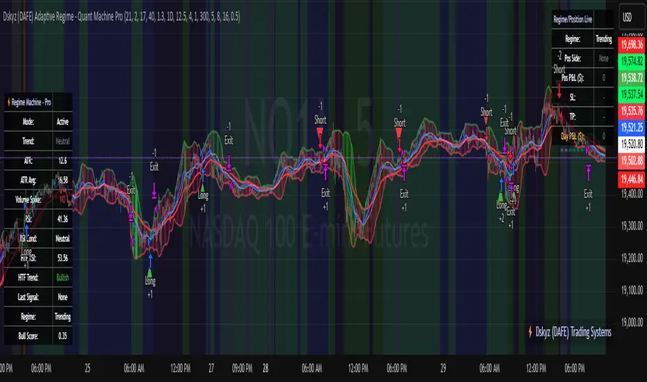
Dskyz (DAFE) Adaptive Regime - Quant Machine ProDskyz (DAFE) Adaptive Regime - Quant Machine Pro:
Buckle up for the Dskyz (DAFE) Adaptive Regime - Quant Machine Pro, is a strategy that’s your ultimate edge for conquering futures markets like ES, MES, NQ, and MNQ. This isn’t just another script—it’s a quant-grade powerhouse, crafted with precision to adapt to market regimes, deliver multi-factor signals, and protect your capital with futures-tuned risk management. With its shimmering DAFE visuals, dual dashboards, and glowing watermark, it turns your charts into a cyberpunk command center, making trading as thrilling as it is profitable.
Unlike generic scripts clogging up the space, the Adaptive Regime is a DAFE original, built from the ground up to tackle the chaos of futures trading. It identifies market regimes (Trending, Range, Volatile, Quiet) using ADX, Bollinger Bands, and HTF indicators, then fires trades based on a weighted scoring system that blends candlestick patterns, RSI, MACD, and more. Add in dynamic stops, trailing exits, and a 5% drawdown circuit breaker, and you’ve got a system that’s as safe as it is aggressive. Whether you’re a newbie or a prop desk pro, this strat’s your ticket to outsmarting the markets. Let’s break down every detail and see why it’s a must-have.
Why Traders Need This Strategy
Futures markets are a gauntlet—fast moves, volatility spikes (like the April 28, 2025 NQ 1k-point drop), and institutional traps that punish the unprepared. Meanwhile, platforms are flooded with low-effort scripts that recycle old ideas with zero innovation. The Adaptive Regime stands tall, offering:
Adaptive Intelligence: Detects market regimes (Trending, Range, Volatile, Quiet) to optimize signals, unlike one-size-fits-all scripts.
Multi-Factor Precision: Combines candlestick patterns, MA trends, RSI, MACD, volume, and HTF confirmation for high-probability trades.
Futures-Optimized Risk: Calculates position sizes based on $ risk (default: $300), with ATR or fixed stops/TPs tailored for ES/MES.
Bulletproof Safety: 5% daily drawdown circuit breaker and trailing stops keep your account intact, even in chaos.
DAFE Visual Mastery: Pulsing Bollinger Band fills, dynamic SL/TP lines, and dual dashboards (metrics + position) make signals crystal-clear and charts a work of art.
Original Craftsmanship: A DAFE creation, built with community passion, not a rehashed clone of generic code.
Traders need this because it’s a complete, adaptive system that blends quant smarts, user-friendly design, and DAFE flair. It’s your edge to trade with confidence, cut through market noise, and leave the copycats in the dust.
Strategy Components
1. Market Regime Detection
The strategy’s brain is its ability to classify market conditions into five regimes, ensuring signals match the environment.
How It Works:
Trending (Regime 1): ADX > 20, fast/slow EMA spread > 0.3x ATR, HTF RSI > 50 or MACD bullish (htf_trend_bull/bear).
Range (Regime 2): ADX < 25, price range < 3% of close, no HTF trend.
Volatile (Regime 3): BB width > 1.5x avg, ATR > 1.2x avg, HTF RSI overbought/oversold.
Quiet (Regime 4): BB width < 0.8x avg, ATR < 0.9x avg.
Other (Regime 5): Default for unclear conditions.
Indicators: ADX (14), BB width (20), ATR (14, 50-bar SMA), HTF RSI (14, daily default), HTF MACD (12,26,9).
Why It’s Brilliant:
Regime detection adapts signals to market context, boosting win rates in trending or volatile conditions.
HTF RSI/MACD add a big-picture filter, rare in basic scripts.
Visualized via gradient background (green for Trending, orange for Range, red for Volatile, gray for Quiet, navy for Other).
2. Multi-Factor Signal Scoring
Entries are driven by a weighted scoring system that combines candlestick patterns, trend, momentum, and volume for robust signals.
Candlestick Patterns:
Bullish: Engulfing (0.5), hammer (0.4 in Range, 0.2 else), morning star (0.2), piercing (0.2), double bottom (0.3 in Volatile, 0.15 else). Must be near support (low ≤ 1.01x 20-bar low) with volume spike (>1.5x 20-bar avg).
Bearish: Engulfing (0.5), shooting star (0.4 in Range, 0.2 else), evening star (0.2), dark cloud (0.2), double top (0.3 in Volatile, 0.15 else). Must be near resistance (high ≥ 0.99x 20-bar high) with volume spike.
Logic: Patterns are weighted higher in specific regimes (e.g., hammer in Range, double bottom in Volatile).
Additional Factors:
Trend: Fast EMA (20) > slow EMA (50) + 0.5x ATR (trend_bull, +0.2); opposite for trend_bear.
RSI: RSI (14) < 30 (rsi_bull, +0.15); > 70 (rsi_bear, +0.15).
MACD: MACD line > signal (12,26,9, macd_bull, +0.15); opposite for macd_bear.
Volume: ATR > 1.2x 50-bar avg (vol_expansion, +0.1).
HTF Confirmation: HTF RSI < 70 and MACD bullish (htf_bull_confirm, +0.2); RSI > 30 and MACD bearish (htf_bear_confirm, +0.2).
Scoring:
bull_score = sum of bullish factors; bear_score = sum of bearish. Entry requires score ≥ 1.0.
Example: Bullish engulfing (0.5) + trend_bull (0.2) + rsi_bull (0.15) + htf_bull_confirm (0.2) = 1.05, triggers long.
Why It’s Brilliant:
Multi-factor scoring ensures signals are confirmed by multiple market dynamics, reducing false positives.
Regime-specific weights make patterns more relevant (e.g., hammers shine in Range markets).
HTF confirmation aligns with the big picture, a quant edge over simplistic scripts.
3. Futures-Tuned Risk Management
The risk system is built for futures, calculating position sizes based on $ risk and offering flexible stops/TPs.
Position Sizing:
Logic: Risk per trade (default: $300) ÷ (stop distance in points * point value) = contracts, capped at max_contracts (default: 5). Point value = tick value (e.g., $12.5 for ES) * ticks per point (4) * contract multiplier (1 for ES, 0.1 for MES).
Example: $300 risk, 8-point stop, ES ($50/point) → 0.75 contracts, rounded to 1.
Impact: Precise sizing prevents over-leverage, critical for micro contracts like MES.
Stops and Take-Profits:
Fixed: Default stop = 8 points, TP = 16 points (2:1 reward/risk).
ATR-Based: Stop = 1.5x ATR (default), TP = 3x ATR, enabled via use_atr_for_stops.
Logic: Stops set at swing low/high ± stop distance; TPs at 2x stop distance from entry.
Impact: ATR stops adapt to volatility, while fixed stops suit stable markets.
Trailing Stops:
Logic: Activates at 50% of TP distance. Trails at close ± 1.5x ATR (atr_multiplier). Longs: max(trail_stop_long, close - ATR * 1.5); shorts: min(trail_stop_short, close + ATR * 1.5).
Impact: Locks in profits during trends, a game-changer in volatile sessions.
Circuit Breaker:
Logic: Pauses trading if daily drawdown > 5% (daily_drawdown = (max_equity - equity) / max_equity).
Impact: Protects capital during black swan events (e.g., April 27, 2025 ES slippage).
Why It’s Brilliant:
Futures-specific inputs (tick value, multiplier) make it plug-and-play for ES/MES.
Trailing stops and circuit breaker add pro-level safety, rare in off-the-shelf scripts.
Flexible stops (ATR or fixed) suit different trading styles.
4. Trade Entry and Exit Logic
Entries and exits are precise, driven by bull_score/bear_score and protected by drawdown checks.
Entry Conditions:
Long: bull_score ≥ 1.0, no position (position_size <= 0), drawdown < 5% (not pause_trading). Calculates contracts, sets stop at swing low - stop points, TP at 2x stop distance.
Short: bear_score ≥ 1.0, position_size >= 0, drawdown < 5%. Stop at swing high + stop points, TP at 2x stop distance.
Logic: Tracks entry_regime for PNL arrays. Closes opposite positions before entering.
Exit Conditions:
Stop-Loss/Take-Profit: Hits stop or TP (strategy.exit).
Trailing Stop: Activates at 50% TP, trails by ATR * 1.5.
Emergency Exit: Closes if price breaches stop (close < long_stop_price or close > short_stop_price).
Reset: Clears stop/TP prices when flat (position_size = 0).
Why It’s Brilliant:
Score-based entries ensure multi-factor confirmation, filtering out weak signals.
Trailing stops maximize profits in trends, unlike static exits in basic scripts.
Emergency exits add an extra safety layer, critical for futures volatility.
5. DAFE Visuals
The visuals are pure DAFE magic, blending function with cyberpunk flair to make signals intuitive and charts stunning.
Shimmering Bollinger Band Fill:
Display: BB basis (20, white), upper/lower (green/red, 45% transparent). Fill pulses (30–50 alpha) by regime, with glow (60–95 alpha) near bands (close ≥ 0.995x upper or ≤ 1.005x lower).
Purpose: Highlights volatility and key levels with a futuristic glow.
Visuals make complex regimes and signals instantly clear, even for newbies.
Pulsing effects and regime-specific colors add a DAFE signature, setting it apart from generic scripts.
BB glow emphasizes tradeable levels, enhancing decision-making.
Chart Background (Regime Heatmap):
Green — Trending Market: Strong, sustained price movement in one direction. The market is in a trend phase—momentum follows through.
Orange — Range-Bound: Market is consolidating or moving sideways, with no clear up/down trend. Great for mean reversion setups.
Red — Volatile Regime: High volatility, heightened risk, and larger/faster price swings—trade with caution.
Gray — Quiet/Low Volatility: Market is calm and inactive, with small moves—often poor conditions for most strategies.
Navy — Other/Neutral: Regime is uncertain or mixed; signals may be less reliable.
Bollinger Bands Glow (Dynamic Fill):
Neon Red Glow — Warning!: Price is near or breaking above the upper band; momentum is overstretched, watch for overbought conditions or reversals.
Bright Green Glow — Opportunity!: Price is near or breaking below the lower band; market could be oversold, prime for bounce or reversal.
Trend Green Fill — Trending Regime: Fills between bands with green when the market is trending, showing clear momentum.
Gold/Yellow Fill — Range Regime: Fills with gold/aqua in range conditions, showing the market is sideways/oscillating.
Magenta/Red Fill — Volatility Spike: Fills with vivid magenta/red during highly volatile regimes.
Blue Fill — Neutral/Quiet: A soft blue glow for other or uncertain market states.
Moving Averages:
Display: Blue fast EMA (20), red slow EMA (50), 2px.
Purpose: Shows trend direction, with trend_dir requiring ATR-scaled spread.
Dynamic SL/TP Lines:
Display: Pulsing colors (red SL, green TP for Trending; yellow/orange for Range, etc.), 3px, with pulse_alpha for shimmer.
Purpose: Tracks stops/TPs in real-time, color-coded by regime.
6. Dual Dashboards
Two dashboards deliver real-time insights, making the strat a quant command center.
Bottom-Left Metrics Dashboard (2x13):
Metrics: Mode (Active/Paused), trend (Bullish/Bearish/Neutral), ATR, ATR avg, volume spike (YES/NO), RSI (value + Oversold/Overbought/Neutral), HTF RSI, HTF trend, last signal (Buy/Sell/None), regime, bull score.
Display: Black (29% transparent), purple title, color-coded (green for bullish, red for bearish).
Purpose: Consolidates market context and signal strength.
Top-Right Position Dashboard (2x7):
Metrics: Regime, position side (Long/Short/None), position PNL ($), SL, TP, daily PNL ($).
Display: Black (29% transparent), purple title, color-coded (lime for Long, red for Short).
Purpose: Tracks live trades and profitability.
Why It’s Brilliant:
Dual dashboards cover market context and trade status, a rare feature.
Color-coding and concise metrics guide beginners (e.g., green “Buy” = go).
Real-time PNL and SL/TP visibility empower disciplined trading.
7. Performance Tracking
Logic: Arrays (regime_pnl_long/short, regime_win/loss_long/short) track PNL and win/loss by regime (1–5). Updated on trade close (barstate.isconfirmed).
Purpose: Prepares for future adaptive thresholds (e.g., adjust bull_score min based on regime performance).
Why It’s Brilliant: Lays the groundwork for self-optimizing logic, a quant edge over static scripts.
Key Features
Regime-Adaptive: Optimizes signals for Trending, Range, Volatile, Quiet markets.
Futures-Optimized: Precise sizing for ES/MES with tick-based risk inputs.
Multi-Factor Signals: Candlestick patterns, RSI, MACD, and HTF confirmation for robust entries.
Dynamic Exits: ATR/fixed stops, 2:1 TPs, and trailing stops maximize profits.
Safe and Smart: 5% drawdown breaker and emergency exits protect capital.
DAFE Visuals: Shimmering BB fill, pulsing SL/TP, and dual dashboards.
Backtest-Ready: Fixed qty and tick calc for accurate historical testing.
How to Use
Add to Chart: Load on a 5min ES/MES chart in TradingView.
Configure Inputs: Set instrument (ES/MES), tick value ($12.5/$1.25), multiplier (1/0.1), risk ($300 default). Enable ATR stops for volatility.
Monitor Dashboards: Bottom-left for regime/signals, top-right for position/PNL.
Backtest: Run in strategy tester to compare regimes.
Live Trade: Connect to Tradovate or similar. Watch for slippage (e.g., April 27, 2025 ES issues).
Replay Test: Try April 28, 2025 NQ drop to see regime shifts and stops.
Disclaimer
Trading futures involves significant risk of loss and is not suitable for all investors. Past performance does not guarantee future results. Backtest results may differ from live trading due to slippage, fees, or market conditions. Use this strategy at your own risk, and consult a financial advisor before trading. Dskyz (DAFE) Trading Systems is not responsible for any losses incurred.
Backtesting:
Frame: 2023-09-20 - 2025-04-29
Slippage: 3
Fee Typical Range (per side, per contract)
CME Exchange $1.14 – $1.20
Clearing $0.10 – $0.30
NFA Regulatory $0.02
Firm/Broker Commis. $0.25 – $0.80 (retail prop)
TOTAL $1.60 – $2.30 per side
Round Turn: (enter+exit) = $3.20 – $4.60 per contract
Final Notes
The Dskyz (DAFE) Adaptive Regime - Quant Machine Pro is more than a strategy—it’s a revolution. Crafted with DAFE’s signature precision, it rises above generic scripts with adaptive regimes, quant-grade signals, and visuals that make trading a thrill. Whether you’re scalping MES or swinging ES, this system empowers you to navigate markets with confidence and style. Join the DAFE crew, light up your charts, and let’s dominate the futures game!
(This publishing will most likely be taken down do to some miscellaneous rule about properly displaying charting symbols, or whatever. Once I've identified what part of the publishing they want to pick on, I'll adjust and repost.)
Use it with discipline. Use it with clarity. Trade smarter.
**I will continue to release incredible strategies and indicators until I turn this into a brand or until someone offers me a contract.
Created by Dskyz, powered by DAFE Trading Systems. Trade smart, trade bold.
Dskyz (DAFE) Aurora Divergence – Quant Master Dskyz (DAFE) Aurora Divergence – Quant Master
Introducing the Dskyz (DAFE) Aurora Divergence – Quant Master , a strategy that’s your secret weapon for mastering futures markets like MNQ, NQ, MES, and ES. Born from the legendary Aurora Divergence indicator, this fully automated system transforms raw divergence signals into a quant-grade trading machine, blending precision, risk management, and cyberpunk DAFE visuals that make your charts glow like a neon skyline. Crafted with care and driven by community passion, this strategy stands out in a sea of generic scripts, offering traders a unique edge to outsmart institutional traps and navigate volatile markets.
The Aurora Divergence indicator was a cult favorite for spotting price-OBV divergences with its aqua and fuchsia orbs, but traders craved a system to act on those signals with discipline and automation. This strategy delivers, layering advanced filters (z-score, ATR, multi-timeframe, session), dynamic risk controls (kill switches, adaptive stops/TPs), and a real-time dashboard to turn insights into profits. Whether you’re a newbie dipping into futures or a pro hunting reversals, this strat’s got your back with a beginner guide, alerts, and visuals that make trading feel like a sci-fi mission. Let’s dive into every detail and see why this original DAFE creation is a must-have.
Why Traders Need This Strategy
Futures markets are a battlefield—fast-paced, volatile, and riddled with institutional games that can wipe out undisciplined traders. From the April 28, 2025 NQ 1k-point drop to sneaky ES slippage, the stakes are high. Meanwhile, platforms are flooded with unoriginal, low-effort scripts that promise the moon but deliver noise. The Aurora Divergence – Quant Master rises above, offering:
Unmatched Originality: A bespoke system built from the ground up, with custom divergence logic, DAFE visuals, and quant filters that set it apart from copycat clutter.
Automation with Precision: Executes trades on divergence signals, eliminating emotional slip-ups and ensuring consistency, even in chaotic sessions.
Quant-Grade Filters: Z-score, ATR, multi-timeframe, and session checks filter out noise, targeting high-probability reversals.
Robust Risk Management: Daily loss and rolling drawdown kill switches, plus ATR-based stops/TPs, protect your capital like a fortress.
Stunning DAFE Visuals: Aqua/fuchsia orbs, aurora bands, and a glowing dashboard make signals intuitive and charts a work of art.
Community-Driven: Evolved from trader feedback, this strat’s a labor of love, not a recycled knockoff.
Traders need this because it’s a complete, original system that blends accessibility, sophistication, and style. It’s your edge to trade smarter, not harder, in a market full of traps and imitators.
1. Divergence Detection (Core Signal Logic)
The strategy’s core is its ability to detect bullish and bearish divergences between price and On-Balance Volume (OBV), pinpointing reversals with surgical accuracy.
How It Works:
Price Slope: Uses linear regression over a lookback (default: 9 bars) to measure price momentum (priceSlope).
OBV Slope: OBV tracks volume flow (+volume if price rises, -volume if falls), with its slope calculated similarly (obvSlope).
Bullish Divergence: Price slope negative (falling), OBV slope positive (rising), and price above 50-bar SMA (trend_ma).
Bearish Divergence: Price slope positive (rising), OBV slope negative (falling), and price below 50-bar SMA.
Smoothing: Requires two consecutive divergence bars (bullDiv2, bearDiv2) to confirm signals, reducing false positives.
Strength: Divergence intensity (divStrength = |priceSlope * obvSlope| * sensitivity) is normalized (0–1, divStrengthNorm) for visuals.
Why It’s Brilliant:
- Divergences catch hidden momentum shifts, often exploited by institutions, giving you an edge on reversals.
- The 50-bar SMA filter aligns signals with the broader trend, avoiding choppy markets.
- Adjustable lookback (min: 3) and sensitivity (default: 1.0) let you tune for different instruments or timeframes.
2. Filters for Precision
Four advanced filters ensure signals are high-probability and market-aligned, cutting through the noise of volatile futures.
Z-Score Filter:
Logic: Calculates z-score ((close - SMA) / stdev) over a lookback (default: 50 bars). Blocks entries if |z-score| > threshold (default: 1.5) unless disabled (useZFilter = false).
Impact: Avoids trades during extreme price moves (e.g., blow-off tops), keeping you in statistically safe zones.
ATR Percentile Volatility Filter:
Logic: Tracks 14-bar ATR in a 100-bar window (default). Requires current ATR > 80th percentile (percATR) to trade (tradeOk).
Impact: Ensures sufficient volatility for meaningful moves, filtering out low-volume chop.
Multi-Timeframe (HTF) Trend Filter:
Logic: Uses a 50-bar SMA on a higher timeframe (default: 60min). Longs require price > HTF MA (bullTrendOK), shorts < HTF MA (bearTrendOK).
Impact: Aligns trades with the bigger trend, reducing counter-trend losses.
US Session Filter:
Logic: Restricts trading to 9:30am–4:00pm ET (default: enabled, useSession = true) using America/New_York timezone.
Impact: Focuses on high-liquidity hours, avoiding overnight spreads and erratic moves.
Evolution:
- These filters create a robust signal pipeline, ensuring trades are timed for optimal conditions.
- Customizable inputs (e.g., zThreshold, atrPercentile) let traders adapt to their style without compromising quality.
3. Risk Management
The strategy’s risk controls are a masterclass in balancing aggression and safety, protecting capital in volatile markets.
Daily Loss Kill Switch:
Logic: Tracks daily loss (dayStartEquity - strategy.equity). Halts trading if loss ≥ $300 (default) and enabled (killSwitch = true, killSwitchActive).
Impact: Caps daily downside, crucial during events like April 27, 2025 ES slippage.
Rolling Drawdown Kill Switch:
Logic: Monitors drawdown (rollingPeak - strategy.equity) over 100 bars (default). Stops trading if > $1000 (rollingKill).
Impact: Prevents prolonged losing streaks, preserving capital for better setups.
Dynamic Stop-Loss and Take-Profit:
Logic: Stops = entry ± ATR * multiplier (default: 1.0x, stopDist). TPs = entry ± ATR * 1.5x (profitDist). Longs: stop below, TP above; shorts: vice versa.
Impact: Adapts to volatility, keeping stops tight but realistic, with TPs targeting 1.5:1 reward/risk.
Max Bars in Trade:
Logic: Closes trades after 8 bars (default) if not already exited.
Impact: Frees capital from stagnant trades, maintaining efficiency.
Kill Switch Buffer Dashboard:
Logic: Shows smallest buffer ($300 - daily loss or $1000 - rolling DD). Displays 0 (red) if kill switch active, else buffer (green).
Impact: Real-time risk visibility, letting traders adjust dynamically.
Why It’s Brilliant:
- Kill switches and ATR-based exits create a safety net, rare in generic scripts.
- Customizable risk inputs (maxDailyLoss, dynamicStopMult) suit different account sizes.
- Buffer metric empowers disciplined trading, a DAFE signature.
4. Trade Entry and Exit Logic
The entry/exit rules are precise, filtered, and adaptive, ensuring trades are deliberate and profitable.
Entry Conditions:
Long Entry: bullDiv2, cooldown passed (canSignal), ATR filter passed (tradeOk), in US session (inSession), no kill switches (not killSwitchActive, not rollingKill), z-score OK (zOk), HTF trend bullish (bullTrendOK), no existing long (lastDirection != 1, position_size <= 0). Closes shorts first.
Short Entry: Same, but for bearDiv2, bearTrendOK, no long (lastDirection != -1, position_size >= 0). Closes longs first.
Adaptive Cooldown: Default 2 bars (cooldownBars). Doubles (up to 10) after a losing trade, resets after wins (dynamicCooldown).
Exit Conditions:
Stop-Loss/Take-Profit: Set per trade (ATR-based). Exits on stop/TP hits.
Other Exits: Closes if maxBarsInTrade reached, ATR filter fails, or kill switch activates.
Position Management: Ensures no conflicting positions, closing opposites before new entries.
Built To Be Reliable and Consistent:
- Multi-filtered entries minimize false signals, a stark contrast to basic scripts.
- Adaptive cooldown prevents overtrading, especially after losses.
- Clean position handling ensures smooth execution, even in fast markets.
5. DAFE Visuals
The visuals are a DAFE hallmark, blending function with clean flair to make signals intuitive and charts stunning.
Aurora Bands:
Display: Bands around price during divergences (bullish: below low, bearish: above high), sized by ATR * bandwidth (default: 0.5).
Colors: Aqua (bullish), fuchsia (bearish), with transparency tied to divStrengthNorm.
Purpose: Highlights divergence zones with a glowing, futuristic vibe.
Divergence Orbs:
Display: Large/small circles (aqua below for bullish, fuchsia above for bearish) when bullDiv2/bearDiv2 and canSignal. Labels show strength (0–1).
Purpose: Pinpoints entries with eye-catching clarity.
Gradient Background:
Display: Green (bullish), red (bearish), or gray (neutral), 90–95% transparent.
Purpose: Sets the market mood without clutter.
Strategy Plots:
- Stop/TP Lines: Red (stops), green (TPs) for active trades.
- HTF MA: Yellow line for trend context.
- Z-Score: Blue step-line (if enabled).
- Kill Switch Warning: Red background flash when active.
What Makes This Next-Level?:
- Visuals make complex signals (divergences, filters) instantly clear, even for beginners.
- DAFE’s unique aesthetic (orbs, bands) sets it apart from generic scripts, reinforcing originality.
- Functional plots (stops, TPs) enhance trade management.
6. Metrics Dashboard
The top-right dashboard (2x8 table) is your command center, delivering real-time insights.
Metrics:
Daily Loss ($): Current loss vs. day’s start, red if > $300.
Rolling DD ($): Drawdown vs. 100-bar peak, red if > $1000.
ATR Threshold: Current percATR, green if ATR exceeds, red if not.
Z-Score: Current value, green if within threshold, red if not.
Signal: “Bullish Div” (aqua), “Bearish Div” (fuchsia), or “None” (gray).
Action: “Consider Buying”/“Consider Selling” (signal color) or “Wait” (gray).
Kill Switch Buffer ($): Smallest buffer to kill switch, green if > 0, red if 0.
Why This Is Important?:
- Consolidates critical data, making decisions effortless.
- Color-coded metrics guide beginners (e.g., green action = go).
- Buffer metric adds transparency, rare in off-the-shelf scripts.
7. Beginner Guide
Beginner Guide: Middle-right table (shown once on chart load), explains aqua orbs (bullish, buy) and fuchsia orbs (bearish, sell).
Key Features:
Futures-Optimized: Tailored for MNQ, NQ, MES, ES with point-value adjustments.
Highly Customizable: Inputs for lookback, sensitivity, filters, and risk settings.
Real-Time Insights: Dashboard and visuals update every bar.
Backtest-Ready: Fixed qty and tick calc for accurate historical testing.
User-Friendly: Guide, visuals, and dashboard make it accessible yet powerful.
Original Design: DAFE’s unique logic and visuals stand out from generic scripts.
How to Use
Add to Chart: Load on a 5min MNQ/ES chart in TradingView.
Configure Inputs: Adjust instrument, filters, or risk (defaults optimized for MNQ).
Monitor Dashboard: Watch signals, actions, and risk metrics (top-right).
Backtest: Run in strategy tester to evaluate performance.
Live Trade: Connect to a broker (e.g., Tradovate) for automation. Watch for slippage (e.g., April 27, 2025 ES issues).
Replay Test: Use bar replay (e.g., April 28, 2025 NQ drop) to test volatility handling.
Disclaimer
Trading futures involves significant risk of loss and is not suitable for all investors. Past performance is not indicative of future results. Backtest results may not reflect live trading due to slippage, fees, or market conditions. Use this strategy at your own risk, and consult a financial advisor before trading. Dskyz (DAFE) Trading Systems is not responsible for any losses incurred.
Backtesting:
Frame: 2023-09-20 - 2025-04-29
Fee Typical Range (per side, per contract)
CME Exchange $1.14 – $1.20
Clearing $0.10 – $0.30
NFA Regulatory $0.02
Firm/Broker Commis. $0.25 – $0.80 (retail prop)
TOTAL $1.60 – $2.30 per side
Round Turn: (enter+exit) = $3.20 – $4.60 per contract
Final Notes
The Dskyz (DAFE) Aurora Divergence – Quant Master isn’t just a strategy—it’s a movement. Crafted with originality and driven by community passion, it rises above the flood of generic scripts to deliver a system that’s as powerful as it is beautiful. With its quant-grade logic, DAFE visuals, and robust risk controls, it empowers traders to tackle futures with confidence and style. Join the DAFE crew, light up your charts, and let’s outsmart the markets together!
(This publishing will most likely be taken down do to some miscellaneous rule about properly displaying charting symbols, or whatever. Once I've identified what part of the publishing they want to pick on, I'll adjust and repost.)
Use it with discipline. Use it with clarity. Trade smarter.
**I will continue to release incredible strategies and indicators until I turn this into a brand or until someone offers me a contract.
Created by Dskyz, powered by DAFE Trading Systems. Trade fast, trade bold.

Dskyz (DAFE) Quantum Sentiment Flux - Beginners Dskyz (DAFE) Quantum Sentiment Flux - Beginners:
Welcome to the Dskyz (DAFE) Quantum Sentiment Flux - Beginners , a strategy and concept that’s your ultimate wingman for trading futures like MNQ, NQ, MES, and ES. This gem combines lightning-fast momentum signals, market sentiment smarts, and bulletproof risk management into a system so intuitive, even newbies can trade like pros. With clean DAFE visuals, preset modes for every vibe, and a revamped dashboard that’s basically a market GPS, this strategy makes futures trading feel like a high-octane sci-fi mission.
Built on the Dskyz (DAFE) legacy of Aurora Divergence, the Quantum Sentiment Flux is designed to empower beginners while giving seasoned traders a lean, sentiment-driven edge. It uses fast/slow EMA crossovers for entries, filters trades with VIX, SPX trends, and sector breadth, and keeps your account safe with adaptive stops and cooldowns. Tuned for more action with faster signals and a slick bottom-left dashboard, this updated version is ready to light up your charts and outsmart institutional traps. Let’s dive into why this strat’s a must-have and break down its brilliance.
Why Traders Need This Strategy
Futures markets are a wild ride—fast moves, volatility spikes (like the April 28, 2025 NQ 1k-point drop), and institutional games that can wreck unprepared traders. Beginners often get lost in complex systems or burned by impulsive trades. The Quantum Sentiment Flux is the antidote, offering:
Dead-Simple Setup: Preset modes (Aggressive, Balanced, Conservative) auto-tune signals, risk, and sizing, so you can trade without a quant degree.
Sentiment Superpower: VIX filter, SPX trend, and sector breadth visuals keep you aligned with market health, dodging chop and riding trends.
Ironclad Safety: Tighter ATR-based stops, 2:1 take-profits, and preset cooldowns protect your capital, even in chaotic sessions.
Next-Level Visuals: Green/red entry triangles, vibrant EMAs, a sector breadth background, and a beefed-up dashboard make signals and context pop.
DAFE Swagger: The clean aesthetics, sleek dashboard—ties it to Dskyz’s elite brand, making your charts a work of art.
Traders need this because it’s a plug-and-play system that blends beginner-friendly simplicity with pro-level market awareness. Whether you’re just starting or scalping 5min MNQ, this strat’s your key to trading with confidence and style.
Strategy Components
1. Core Signal Logic (High-Speed Momentum)
The strategy’s engine is a momentum-based system using fast and slow Exponential Moving Averages (EMAs), now tuned for faster, more frequent trades.
How It Works:
Fast/Slow EMAs: Fast EMA (Aggressive: 5, Balanced: 7, Conservative: 9 bars) and slow EMA (12/14/18 bars) track short-term vs. longer-term momentum.
Crossover Signals:
Buy: Fast EMA crosses above slow EMA, and trend_dir = 1 (fast EMA > slow EMA + ATR * strength threshold).
Sell: Fast EMA crosses below slow EMA, and trend_dir = -1 (fast EMA < slow EMA - ATR * strength threshold).
Strength Filter: ma_strength = fast EMA - slow EMA must exceed an ATR-scaled threshold (Aggressive: 0.15, Balanced: 0.18, Conservative: 0.25) for robust signals.
Trend Direction: trend_dir confirms momentum, filtering out weak crossovers in choppy markets.
Evolution:
Faster EMAs (down from 7–10/21–50) catch short-term trends, perfect for active futures markets.
Lower strength thresholds (0.15–0.25 vs. 0.3–0.5) make signals more sensitive, boosting trade frequency without sacrificing quality.
Preset tuning ensures beginners get optimized settings, while pros can tweak via mode selection.
2. Market Sentiment Filters
The strategy leans hard into market sentiment with a VIX filter, SPX trend analysis, and sector breadth visuals, keeping trades aligned with the big picture.
VIX Filter:
Logic: Blocks long entries if VIX > threshold (default: 20, can_long = vix_close < vix_limit). Shorts are always allowed (can_short = true).
Impact: Prevents longs during high-fear markets (e.g., VIX spikes in crashes), while allowing shorts to capitalize on downturns.
SPX Trend Filter:
Logic: Compares S&P 500 (SPX) close to its SMA (Aggressive: 5, Balanced: 8, Conservative: 12 bars). spx_trend = 1 (UP) if close > SMA, -1 (DOWN) if < SMA, 0 (FLAT) if neutral.
Impact: Provides dashboard context, encouraging trades that align with market direction (e.g., longs in UP trend).
Sector Breadth (Visual):
Logic: Tracks 10 sector ETFs (XLK, XLF, XLE, etc.) vs. their SMAs (same lengths as SPX). Each sector scores +1 (bullish), -1 (bearish), or 0 (neutral), summed as breadth (-10 to +10).
Display: Green background if breadth > 4, red if breadth < -4, else neutral. Dashboard shows sector trends (↑/↓/-).
Impact: Faster SMA lengths make breadth more responsive, reflecting sector rotations (e.g., tech surging, energy lagging).
Why It’s Brilliant:
- VIX filter adds pro-level volatility awareness, saving beginners from panic-driven losses.
- SPX and sector breadth give a 360° view of market health, boosting signal confidence (e.g., green BG + buy signal = high-probability trade).
- Shorter SMAs make sentiment visuals react faster, perfect for 5min charts.
3. Risk Management
The risk controls are a fortress, now tighter and more dynamic to support frequent trading while keeping accounts safe.
Preset-Based Risk:
Aggressive: Fast EMAs (5/12), tight stops (1.1x ATR), 1-bar cooldown. High trade frequency, higher risk.
Balanced: EMAs (7/14), 1.2x ATR stops, 1-bar cooldown. Versatile for most traders.
Conservative: EMAs (9/18), 1.3x ATR stops, 2-bar cooldown. Safer, fewer trades.
Impact: Auto-scales risk to match style, making it foolproof for beginners.
Adaptive Stops and Take-Profits:
Logic: Stops = entry ± ATR * atr_mult (1.1–1.3x, down from 1.2–2.0x). Take-profits = entry ± ATR * take_mult (2x stop distance, 2:1 reward/risk). Longs: stop below entry, TP above; shorts: vice versa.
Impact: Tighter stops increase trade turnover while maintaining solid risk/reward, adapting to volatility.
Trade Cooldown:
Logic: Preset-driven (Aggressive/Balanced: 1 bar, Conservative: 2 bars vs. old user-input 2). Ensures bar_index - last_trade_bar >= cooldown.
Impact: Faster cooldowns (especially Aggressive/Balanced) allow more trades, balanced by VIX and strength filters.
Contract Sizing:
Logic: User sets contracts (default: 1, max: 10), no preset cap (unlike old 7/5/3 suggestion).
Impact: Flexible but risks over-leverage; beginners should stick to low contracts.
Built To Be Reliable and Consistent:
- Tighter stops and faster cooldowns make it a high-octane system without blowing up accounts.
- Preset-driven risk removes guesswork, letting newbies trade confidently.
- 2:1 TPs ensure profitable trades outweigh losses, even in volatile sessions like April 27, 2025 ES slippage.
4. Trade Entry and Exit Logic
The entry/exit rules are simple yet razor-sharp, now with VIX filtering and faster signals:
Entry Conditions:
Long Entry: buy_signal (fast EMA crosses above slow EMA, trend_dir = 1), no position (strategy.position_size = 0), cooldown passed (can_trade), and VIX < 20 (can_long). Enters with user-defined contracts.
Short Entry: sell_signal (fast EMA crosses below slow EMA, trend_dir = -1), no position, cooldown passed, can_short (always true).
Logic: Tracks last_entry_bar for visuals, last_trade_bar for cooldowns.
Exit Conditions:
Stop-Loss/Take-Profit: ATR-based stops (1.1–1.3x) and TPs (2x stop distance). Longs exit if price hits stop (below) or TP (above); shorts vice versa.
No Other Exits: Keeps it straightforward, relying on stops/TPs.
5. DAFE Visuals
The visuals are pure DAFE magic, blending clean function with informative metrics utilized by professionals, now enhanced by faster signals and a responsive breadth background:
EMA Plots:
Display: Fast EMA (blue, 2px), slow EMA (orange, 2px), using faster lengths (5–9/12–18).
Purpose: Highlights momentum shifts, with crossovers signaling entries.
Sector Breadth Background:
Display: Green (90% transparent) if breadth > 4, red (90%) if breadth < -4, else neutral.
Purpose: Faster breadth_sma_len (5–12 vs. 10–50) reflects sector shifts in real-time, reinforcing signal strength.
- Visuals are intuitive, turning complex signals into clear buy/sell cues.
- Faster breadth background reacts to market rotations (e.g., tech vs. energy), giving a pro-level edge.
6. Sector Breadth Dashboard
The new bottom-left dashboard is a game-changer, a 3x16 table (black/gray theme) that’s your market command center:
Metrics:
VIX: Current VIX (red if > 20, gray if not).
SPX: Trend as “UP” (green), “DOWN” (red), or “FLAT” (gray).
Trade Longs: “OK” (green) if VIX < 20, “BLOCK” (red) if not.
Sector Breadth: 10 sectors (Tech, Financial, etc.) with trend arrows (↑ green, ↓ red, - gray).
Placeholder Row: Empty for future metrics (e.g., ATR, breadth score).
Purpose: Consolidates regime, volatility, market trend, and sector data, making decisions a breeze.
- VIX and SPX metrics add context, helping beginners avoid bad trades (e.g., no longs if “BLOCK”).
Sector arrows show market health at a glance, like a cheat code for sentiment.
Key Features
Beginner-Ready: Preset modes and clear visuals make futures trading a breeze.
Sentiment-Driven: VIX filter, SPX trend, and sector breadth keep you in sync with the market.
High-Frequency: Faster EMAs, tighter stops, and short cooldowns boost trade volume.
Safe and Smart: Adaptive stops/TPs and cooldowns protect capital while maximizing wins.
Visual Mastery: DAFE’s clean flair, EMAs, dashboard—makes trading fun and clear.
Backtestable: Lean code and fixed qty ensure accurate historical testing.
How to Use
Add to Chart: Load on a 5min MNQ/ES chart in TradingView.
Pick Preset: Aggressive (scalping), Balanced (versatile), or Conservative (safe). Balanced is default.
Set Contracts: Default 1, max 10. Stick low for safety.
Check Dashboard: Bottom-left shows preset, VIX, SPX, and sectors. “OK” + green breadth = strong buy.
Backtest: Run in strategy tester to compare modes.
Live Trade: Connect to Tradovate or similar. Watch for slippage (e.g., April 27, 2025 ES issues).
Replay Test: Try April 28, 2025 NQ drop to see VIX filter and stops in action.
Why It’s Brilliant
The Dskyz (DAFE) Quantum Sentiment Flux - Beginners is a masterpiece of simplicity and power. It takes pro-level tools—momentum, VIX, sector breadth—and wraps them in a system anyone can run. Faster signals and tighter stops make it a trading machine, while the VIX filter and dashboard keep you ahead of market chaos. The DAFE visuals and bottom-left command center turn your chart into a futuristic cockpit, guiding you through every trade. For beginners, it’s a safe entry to futures; for pros, it’s a scalping beast with sentiment smarts. This strat doesn’t just trade—it transforms how you see the market.
Final Notes
This is more than a strategy—it’s your launchpad to mastering futures with Dskyz (DAFE) flair. The Quantum Sentiment Flux blends accessibility, speed, and market savvy to help you outsmart the game. Load it, watch those triangles glow, and let’s make the markets your canvas!
Official Statement from Pine Script Team
(see TradingView help docs and forums):
"This warning may appear when you call functions such as ta.sma inside a request.security in a loop. There is no runtime impact. If you need to loop through a dynamic list of tickers, this cannot be avoided in the present version... Values will still be correct. Ignore this warning in such contexts."
(This publishing will most likely be taken down do to some miscellaneous rule about properly displaying charting symbols, or whatever. Once I've identified what part of the publishing they want to pick on, I'll adjust and repost.)
Use it with discipline. Use it with clarity. Trade smarter.
**I will continue to release incredible strategies and indicators until I turn this into a brand or until someone offers me a contract.
Created by Dskyz, powered by DAFE Trading Systems. Trade fast, trade bold.
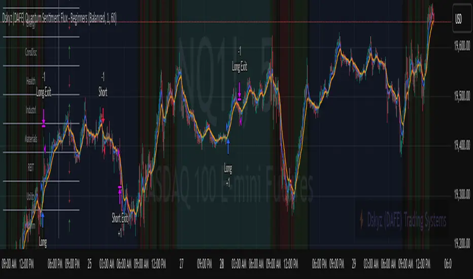
RSI_Heikinashi📜 Title:
Heikin-Ashi RSI Candle Plot with Multi-Timeframe Analysis and EMA Overlay
📖 Full Description:
This is an original custom indicator that transforms the traditional Relative Strength Index (RSI) into a Heikin-Ashi (HA) candle representation, allowing traders to visualize RSI trends with greater clarity, less noise, and multi-timeframe perspective.
🛠️ Core Concept and Original Method:
Rather than plotting a single RSI line, this script recalculates RSI into a Heikin-Ashi candle format, using a double EMA smoothing method on the RSI data itself.
Here's how the transformation works:
RSI Calculation:
RSI is computed traditionally using Wilder's Moving Average (RMA) for smoothing gains and losses.
The RSI period and price source are fully customizable (default length = 28, source = close).
Heikin-Ashi Style Smoothing (applied to RSI):
The HA Close is calculated as the EMA of the average between the current RSI and previous HA Close.
The HA Open is calculated as the EMA of the average between the previous HA Open and the current HA Close.
The HA High and HA Low are dynamically calculated based on the maximum/minimum values of the current RSI, HA Open, and HA Close.
Smoothing is done via 5-period EMA, which adds a unique layer of trend smoothing without traditional price-based HA calculation.
Multi-Timeframe Comparison:
In addition to plotting the chart timeframe HA RSI, the indicator retrieves the 1-hour timeframe HA RSI using request.security.
This allows traders to align trades with higher timeframe RSI trends, a powerful technique for multi-timeframe confirmation.
50 EMA Overlay:
A 50-period Exponential Moving Average (EMA) is plotted over both the chart timeframe HA RSI and the 1-hour HA RSI.
EMA acts as a trend filter or dynamic support/resistance for RSI behavior.
RSI Bands and Visual Aids:
Standard RSI bands at 70 (Overbought), 50 (Midline), and 30 (Oversold) are plotted.
A shaded background between the 30–70 levels helps highlight RSI range-bound movements versus breakout momentum.
🔥 Why this script is original and useful:
Unique Application:
This is not a simple RSI plot or standard Heikin-Ashi candle — it is a specialized smoothing method applied directly to RSI values for a clearer, noise-reduced momentum reading.
Multi-Timeframe Advantage:
Unlike typical RSI indicators, it includes a 1-hour timeframe comparison alongside the chart timeframe, improving decision-making across intraday and swing strategies.
Advanced Smoothing Logic:
Double EMA smoothing of RSI and HA-style recalculations offer a much smoother signal than traditional RSI or basic RSI/EMA crossovers.
Visualized Trend Strength:
Using colored candles instead of just a line enhances readability and gives an intuitive sense of momentum direction, strength, and possible reversals.
Fully Customizable:
Traders can adjust the RSI period and source depending on asset volatility or timeframe preferences.
📋 How to Use:
Look for HA RSI candles color changes for early momentum shifts.
Use the 50 EMA crossovers on HA RSI to confirm larger trend changes.
Compare chart timeframe vs 1H timeframe HA RSI for stronger signal alignment.
Watch for overbought/oversold breaks beyond the 70/30 bands for trade entries or exits.
⚙️ Inputs:
RSI Length (Default: 28)
RSI Source (Default: Close)
📢 Important Note:
This script is originally conceptualized and custom-built.
It is not a mashup of existing open-source indicators and introduces a new smoothing technique for RSI visualization.
🙏 Credits:
Script developed by Sri_RSI.
Williams R Zone Scalper v1.0[BullByte]Originality & Usefulness
Unlike standard Williams R cross-over scripts, this strategy layers five dynamic filters—moving-average trend, Supertrend, Choppiness Index, Bollinger Band Width, and volume validation —and presents a real-time dashboard with equity, PnL, filter status, and key indicator values. No other public Pine script combines these elements with toggleable filters and a custom dashboard. In backtests (BTC/USD (Binance), 5 min, 24 Mar 2025 → 28 Apr 2025), adding these filters turned a –2.09 % standalone Williams R into a +5.05 % net winner while cutting maximum drawdown in half.
---
What This Script Does
- Monitors Williams R (length 14) for overbought/oversold reversals.
- Applies up to five dynamic filters to confirm trend strength and volatility direction:
- Moving average (SMA/EMA/WMA/HMA)
- Supertrend line
- Choppiness Index (CI)
- Bollinger Band Width (BBW)
- Volume vs. its 50-period MA
- Plots blue arrows for Long entries (R crosses above –80 + all filters green) and red arrows for Short entries (R crosses below –20 + all filters green).
- Optionally sets dynamic ATR-based stop-loss (1.5×ATR) and take-profit (2×ATR).
- Shows a dashboard box with current position, equity, PnL, filter status, and real-time Williams R / MA/volume values.
---
Backtest Summary (BTC/USD(Binance), 5 min, 24 Mar 2025 → 28 Apr 2025)
• Total P&L : +50.70 USD (+5.05 %)
• Max Drawdown : 31.93 USD (3.11 %)
• Total Trades : 198
• Win Rate : 55.05 % (109/89)
• Profit Factor : 1.288
• Commission : 0.01 % per trade
• Slippage : 0 ticks
Even in choppy March–April, this multi-filter approach nets +5 % with a robust risk profile, compared to –2.09 % and higher drawdown for Williams R alone.
---
Williams R Alone vs. Multi-Filter Version
• Total P&L :
– Williams R alone → –20.83 USD (–2.09 %)
– Multi-Filter → +50.70 USD (+5.05 %)
• Max Drawdown :
– Williams R alone → 62.13 USD (6.00 %)
– Multi-Filter → 31.93 USD (3.11 %)
• Total Trades : 543 vs. 198
• Win Rate : 60.22 % vs. 55.05 %
• Profit Factor : 0.943 vs. 1.288
---
Inputs & What They Control
- wrLen (14): Williams R look-back
- maType (EMA): Trend filter type (SMA, EMA, WMA, HMA)
- maLen (20): Moving-average period
- useChop (true): Toggle Choppiness Index filter
- ciLen (12): CI look-back length
- chopThr (38.2): CI threshold (below = trending)
- useVol (true): Toggle volume-above-average filter
- volMaLen (50): Volume MA period
- useBBW (false): Toggle Bollinger Band Width filter
- bbwMaLen (50): BBW MA period
- useST (false): Toggle Supertrend filter
- stAtrLen (10): Supertrend ATR length
- stFactor (3.0): Supertrend multiplier
- useSL (false): Toggle ATR-based SL/TP
- atrLen (14): ATR period for SL/TP
- slMult (1.5): SL = slMult × ATR
- tpMult (2.0): TP = tpMult × ATR
---
How to Read the Chart
- Blue arrow (Long): Williams R crosses above –80 + all enabled filters green
- Red arrow (Short) : Williams R crosses below –20 + all filters green
- Dashboard box:
- Top : position and equity
- Next : cumulative PnL in USD & %
- Middle : green/white dots for each filter (green=passing, white=disabled)
- Bottom : Williams R, MA, and volume current values
---
Usage Tips
- Add the script : Indicators → My Scripts → Williams R Zone Scalper v1.0 → Add to BTC/USD chart on 5 min.
- Defaults : Optimized for BTC/USD.
- Forex majors : Raise `chopThr` to ~42.
- Stocks/high-beta : Enable `useBBW`.
- Enable SL/TP : Toggle `useSL`; stop-loss = 1.5×ATR, take-profit = 2×ATR apply automatically.
---
Common Questions
- * Why not trade every Williams R reversal?*
Raw Williams R whipsaws in sideways markets. Choppiness and volume filters reduce false entries.
- *Can I use on 1 min or 15 min?*
Yes—adjust ATR length or thresholds accordingly. Defaults target 5 min scalping.
- *What if all filters are on?*
Fewer arrows, higher-quality signals. Expect ~10 % boost in average win size.
---
Disclaimer & License
Trading carries risk of loss. Use this script “as is” under the Mozilla Public License 2.0 (mozilla.org). Always backtest, paper-trade, and adjust risk settings to your own profile.
---
Credits & References
- Pine Script v6, using TradingView’s built-in `ta.supertrend()`.
- TradingView House Rules: www.tradingview.com
Goodluck!
BullByte
Uptrick Signal Density Cloud🟪 Introduction
The Uptrick Signal Density Cloud is designed to track market direction and highlight potential reversals or shifts in momentum. It plots two smoothed lines on the chart and fills the space between them (often called a “cloud”). The bars on the chart change color depending on bullish or bearish conditions, and small triangles appear when certain reversal criteria are met. A metrics table displays real-time values for easy reference.
🟩 Why These Features Have Been Linked Together
1) Dual-Line Structure
Two separate lines represent shorter- and longer-term market tendencies. Linking them in one tool allows traders to view both near-term changes and the broader directional bias in a single glance.
2) Smoothed Averages
The script offers multiple smoothing methods—exponential, simple, hull, and an optimized approach—to reduce noise. Using more than one type of moving average can help balance responsiveness with stability.
3) Density Cloud Concept
Shading the region between the two lines highlights the gap or “thickness.” A wider gap typically signals stronger momentum, while a narrower gap could indicate a weakening trend or potential market indecision. When the cloud is too wide and crosses a certain threshold defined by the user, it indicates a possible reversal. When the cloud is too narrow it may indicate a potential breakout.
🟪 Why Use This Indicator
• Trend Visibility: The color-coded lines and bars make it easier to distinguish bullish from bearish conditions.
• Momentum Tracking: Thicker cloud regions suggest stronger separation between the faster and slower lines, potentially indicating robust momentum.
• Possible Reversal Alerts: Small triangles appear within thick zones when the indicator detects a crossover, drawing attention to key moments of potential trend change.
• Quick Reference Table: A metrics table shows line values, bullish or bearish status, and cloud thickness without needing to hover over chart elements.
🟩 Inputs
1) First Smoothing Length (length1)
Default: 14
Defines the lookback period for the faster line. Lower values make the line respond more quickly to price changes.
2) Second Smoothing Length (length2)
Default: 28
Defines the lookback period for the slower line or one of the moving averages in optimized mode. It generally responds more slowly than the faster line.
3) Extra Smoothing Length (extraLength)
Default: 50
A medium-term period commonly seen in technical analysis. In optimized mode, it helps add broader perspective to the combined lines.
4) Source (source)
Default: close
Specifies the price data (for example, open, high, low, or a custom source) used in the calculations.
5) Cloud Type (cloudType)
Options: Optimized, EMA, SMA, HMA
Determines the smoothing method used for the lines. “Optimized” blends multiple exponential averages at different lengths.
6) Cloud Thickness Threshold (thicknessThreshold)
Default: 0.5
Sets the minimum separation between the two lines to qualify as a “thick” zone, indicating potentially stronger momentum.
🟪 Core Components
1) Faster and Slower Lines
Each line is smoothed according to user preferences or the optimized technique. The faster line typically reacts more quickly, while the slower line provides a broader overview.
2) Filled Density Cloud
The space between the two lines is filled to visualize in which direction the market is trending.
3) Color-Coded Bars
Price bars adopt bullish or bearish colors based on which line is on top, providing an immediate sense of trend direction.
4) Reversal Triangles
When the cloud is thick (exceeding the threshold) and the lines cross in the opposite direction, small triangles appear, signaling a possible market shift.
5) Metrics Table
A compact table shows the current values of both lines, their bullish/bearish statuses, the cloud thickness, and whether the cloud is in a “reversal zone.”
🟩 Calculation Process
1) Raw Averages
Depending on the mode, standard exponential, simple, hull, or “optimized” exponential blends are calculated.
2) Optimized Averages (if selected)
The faster line is the average of three exponential moving averages using length1, length2, and extraLength.
The slower line similarly uses those same lengths multiplied by 1.5, then averages them together for broader smoothing.
3) Difference and Threshold
The absolute gap between the two lines is measured. When it exceeds thicknessThreshold, the cloud is considered thick.
4) Bullish or Bearish Determination
If sma1 (the faster line) is above sma2 (the slower line), conditions are deemed bullish; otherwise, they are bearish. This distinction is reflected in both bar colors and cloud shading.
5) Reversal Markers
In thick zones, a crossover triggers a triangle at the point of potential reversal, alerting traders to a possible trend change.
🟪 Smoothing Methods
1) Exponential (EMA)
Prioritizes recent data for quicker responsiveness.
2) Simple (SMA)
Takes a straightforward average of the chosen period, smoothing price action but often lagging more in volatile markets.
3) Hull (HMA)
Employs a specialized formula to reduce lag while maintaining smoothness.
4) Optimized (Blended Exponential)
Combines multiple EMA calculations to strike a balance between responsiveness and noise reduction.
🟩 Cloud Logic and Reversal Zones
Cloud thickness above the defined threshold typically signals exceeding momentum and can lead to a quick reversal. During these thick periods, if the width exceeds the defined threshold, small triangles mark potential reversal points. In order for the reversal shape to show, the color of the cloud has to be the opposite. So, for example, if the cloud is bearish, and exceeds momentum, defined by the user, a bullish signal appears. The opposite conditions for a bullish signal. This approach can help traders focus on notable changes rather than minor oscillations.
🟪 Bar Coloring and Layered Lines
Bars take on bullish or bearish tints, matching the faster line’s position relative to the slower line. The lines themselves are plotted multiple times with varying opacities, creating a layered, glowing look that enhances visibility without affecting calculations.
🟩 The Metrics Table
Located in the top-right corner of the chart, this table displays:
• SMA1 and SMA2 current values.
• Bullish or bearish alignment for each line.
• Cloud thickness.
• Reversal zone status (in or out of zone).
This numeric readout allows for a quick data check without hovering over the chart.
🟪 Why These Specific Moving Average Lengths Are Used
Default lengths of 14, 28, and 50 are common in technical analysis. Fourteen captures near-term price movement without overreacting. Twenty-eight, roughly double 14, provides a moderate smoothing level. Fifty is widely regarded as a medium-term benchmark. Multiplying each length by 1.5 for the slower line enhances separation when combined with the faster line.
🟩 Originality and Usefulness
• Multi-Layered Smoothing. The user can select from several moving average modes, including a unique “optimized” blend, possibly reducing random fluctuations in the market data.
• Combined Visual and Numeric Clarity. Bars, clouds, and a real-time table merge into a single interface, enabling efficient trend analysis.
• Focus on Significant Shifts. Thick cloud zones and triangles draw attention to potentially stronger momentum changes and plausible reversals.
• Flexible Across Markets. The adjustable lengths and threshold can be tuned to different asset classes (stocks, forex, commodities, crypto) and timeframes.
By integrating multiple technical concepts—cloud-based trend detection, color coding, reversal markers, and an immediate reference table—the Uptrick Signal Density Cloud aims to streamline chart reading and decision-making.
🟪 Additional Considerations
• Timeframes. Intraday, daily, and weekly charts each yield different signals. Adjust the smoothing lengths and threshold to suit specific trading horizons.
• Market Types. Though applicable across asset classes, parameters might need tweaking to address the volatility of commodities, forex pairs, or cryptocurrencies.
• Confirmation Tools. Pairing this indicator with volume studies or support/resistance analysis can improve the reliability of signals.
• Potential Limitations. No indicator is foolproof; sudden market shifts or choppy conditions may reduce accuracy. Cautious position sizing and risk management remain essential.
🟩 Disclaimers
The Uptrick Signal Density Cloud relies on historical price data and may lag sudden moves or provide false positives in ranging conditions. Always combine it with other analytical techniques and sound risk management. This script is offered for educational purposes only and should not be considered financial advice.
🟪 Conclusion
The Uptrick Signal Density Cloud blends trend identification, momentum assessment, and potential reversal alerts in a single, user-friendly tool. With customizable smoothing methods and a focus on cloud thickness, it visually highlights important market conditions. While it cannot guarantee predictive accuracy, it can serve as a comprehensive reference for traders seeking both a quick snapshot of the current trend and deeper insights into market dynamics.

Ensemble Alerts█ OVERVIEW
This indicator creates highly customizable alert conditions and messages by combining several technical conditions into groups , which users can specify directly from the "Settings/Inputs" tab. It offers a flexible framework for building and testing complex alert conditions without requiring code modifications for each adjustment.
█ CONCEPTS
Ensemble analysis
Ensemble analysis is a form of data analysis that combines several "weaker" models to produce a potentially more robust model. In a trading context, one of the most prevalent forms of ensemble analysis is the aggregation (grouping) of several indicators to derive market insights and reinforce trading decisions. With this analysis, traders typically inspect multiple indicators, signaling trade actions when specific conditions or groups of conditions align.
Simplifying ensemble creation
Combining indicators into one or more ensembles can be challenging, especially for users without programming knowledge. It usually involves writing custom scripts to aggregate the indicators and trigger trading alerts based on the confluence of specific conditions. Making such scripts customizable via inputs poses an additional challenge, as it often involves complicated input menus and conditional logic.
This indicator addresses these challenges by providing a simple, flexible input menu where users can easily define alert criteria by listing groups of conditions from various technical indicators in simple text boxes . With this script, you can create complex alert conditions intuitively from the "Settings/Inputs" tab without ever writing or modifying a single line of code. This framework makes advanced alert setups more accessible to non-coders. Additionally, it can help Pine programmers save time and effort when testing various condition combinations.
█ FEATURES
Configurable alert direction
The "Direction" dropdown at the top of the "Settings/Inputs" tab specifies the allowed direction for the alert conditions. There are four possible options:
• Up only : The indicator only evaluates upward conditions.
• Down only : The indicator only evaluates downward conditions.
• Up and down (default): The indicator evaluates upward and downward conditions, creating alert triggers for both.
• Alternating : The indicator prevents alert triggers for consecutive conditions in the same direction. An upward condition must be the first occurrence after a downward condition to trigger an alert, and vice versa for downward conditions.
Flexible condition groups
This script features six text inputs where users can define distinct condition groups (ensembles) for their alerts. An alert trigger occurs if all the conditions in at least one group occur.
Each input accepts a comma-separated list of numbers with optional spaces (e.g., "1, 4, 8"). Each listed number, from 1 to 35, corresponds to a specific individual condition. Below are the conditions that the numbers represent:
1 — RSI above/below threshold
2 — RSI below/above threshold
3 — Stoch above/below threshold
4 — Stoch below/above threshold
5 — Stoch K over/under D
6 — Stoch K under/over D
7 — AO above/below threshold
8 — AO below/above threshold
9 — AO rising/falling
10 — AO falling/rising
11 — Supertrend up/down
12 — Supertrend down/up
13 — Close above/below MA
14 — Close below/above MA
15 — Close above/below open
16 — Close below/above open
17 — Close increase/decrease
18 — Close decrease/increase
19 — Close near Donchian top/bottom (Close > (Mid + HH) / 2)
20 — Close near Donchian bottom/top (Close < (Mid + LL) / 2)
21 — New Donchian high/low
22 — New Donchian low/high
23 — Rising volume
24 — Falling volume
25 — Volume above average (Volume > SMA(Volume, 20))
26 — Volume below average (Volume < SMA(Volume, 20))
27 — High body to range ratio (Abs(Close - Open) / (High - Low) > 0.5)
28 — Low body to range ratio (Abs(Close - Open) / (High - Low) < 0.5)
29 — High relative volatility (ATR(7) > ATR(40))
30 — Low relative volatility (ATR(7) < ATR(40))
31 — External condition 1
32 — External condition 2
33 — External condition 3
34 — External condition 4
35 — External condition 5
These constituent conditions fall into three distinct categories:
• Directional pairs : The numbers 1-22 correspond to pairs of opposing upward and downward conditions. For example, if one of the inputs includes "1" in the comma-separated list, that group uses the "RSI above/below threshold" condition pair. In this case, the RSI must be above a high threshold for the group to trigger an upward alert, and the RSI must be below a defined low threshold to trigger a downward alert.
• Non-directional filters : The numbers 23-30 correspond to conditions that do not represent directional information. These conditions act as filters for both upward and downward alerts. Traders often use non-directional conditions to refine trending or mean reversion signals. For instance, if one of the input lists includes "30", that group uses the "Low relative volatility" condition. The group can trigger an upward or downward alert only if the 7-period Average True Range (ATR) is below the 40-period ATR.
• External conditions : The numbers 31-35 correspond to external conditions based on the plots from other indicators on the chart. To set these conditions, use the source inputs in the "External conditions" section near the bottom of the "Settings/Inputs" tab. The external value can represent an upward, downward, or non-directional condition based on the following logic:
▫ Any value above 0 represents an upward condition.
▫ Any value below 0 represents a downward condition.
▫ If the checkbox next to the source input is selected, the condition becomes non-directional . Any group that uses the condition can trigger upward or downward alerts only if the source value is not 0.
To learn more about using plotted values from other indicators, see this article in our Help Center and the Source input section of our Pine Script™ User Manual.
Group markers
Each comma-separated list represents a distinct group , where all the listed conditions must occur to trigger an alert. This script assigns preset markers (names) to each condition group to make the active ensembles easily identifiable in the generated alert messages and labels. The markers assigned to each group use the format "M", where "M" is short for "Marker" and "x" is the group number. The titles of the inputs at the top of the "Settings/Inputs" tab show these markers for convenience.
For upward conditions, the labels and alert messages show group markers with upward triangles (e.g., "M1▲"). For downward conditions, they show markers with downward triangles (e.g., "M1▼").
NOTE: By default, this script populates the "M1" field with a pre-configured list for a mean reversion group ("2,18,24,28"). The other fields are empty. If any "M*" input does not contain a value, the indicator ignores it in the alert calculations.
Custom alert messages
By default, the indicator's alert message text contains the activated markers and their direction as a comma-separated list. Users can override this message for upward or downward alerts with the two text fields at the bottom of the "Settings/Inputs" tab. When the fields are not empty , the alerts use that text instead of the default marker list.
NOTE: This script generates alert triggers, not the alerts themselves. To set up an alert based on this script's conditions, open the "Create Alert" dialog box, then select the "Ensemble Alerts" and "Any alert() function call" options in the "Condition" tabs. See the Alerts FAQ in our Pine Script™ User Manual for more information.
Condition visualization
This script offers organized visualizations of its conditions, allowing users to inspect the behaviors of each condition alongside the specified groups. The key visual features include:
1) Conditional plots
• The indicator plots the history of each individual condition, excluding the external conditions, as circles at different levels. Opposite conditions appear at positive and negative levels with the same absolute value. The plots for each condition show values only on the bars where they occur.
• Each condition's plot is color-coded based on its type. Aqua and orange plots represent opposing directional conditions, and purple plots represent non-directional conditions. The titles of the plots also contain the condition numbers to which they apply.
• The plots in the separate pane can be turned on or off with the "Show plots in pane" checkbox near the top of the "Settings/Inputs" tab. This input only toggles the color-coded circles, which reduces the graphical load. If you deactivate these visuals, you can still inspect each condition from the script's status line and the Data Window.
• As a bonus, the indicator includes "Up alert" and "Down alert" plots in the Data Window, representing the combined upward and downward ensemble alert conditions. These plots are also usable in additional indicator-on-indicator calculations.
2) Dynamic labels
• The indicator draws a label on the main chart pane displaying the activated group markers (e.g., "M1▲") each time an alert condition occurs.
• The labels for upward alerts appear below chart bars. The labels for downward alerts appear above the bars.
NOTE: This indicator can display up to 500 labels because that is the maximum allowed for a single Pine script.
3) Background highlighting
• The indicator can highlight the main chart's background on bars where upward or downward condition groups activate. Use the "Highlight background" inputs in the "Settings/Inputs" tab to enable these highlights and customize their colors.
• Unlike the dynamic labels, these background highlights are available for all chart bars, irrespective of the number of condition occurrences.
█ NOTES
• This script uses Pine Script™ v6, the latest version of TradingView's programming language. See the Release notes and Migration guide to learn what's new in v6 and how to convert your scripts to this version.
• This script imports our new Alerts library, which features functions that provide high-level simplicity for working with complex compound conditions and alerts. We used the library's `compoundAlertMessage()` function in this indicator. It evaluates items from "bool" arrays in groups specified by an array of strings containing comma-separated index lists , returning a tuple of "string" values containing the marker of each activated group.
• The script imports the latest version of the ta library to calculate several technical indicators not included in the built-in `ta.*` namespace, including Double Exponential Moving Average (DEMA), Triple Exponential Moving Average (TEMA), Fractal Adaptive Moving Average (FRAMA), Tilson T3, Awesome Oscillator (AO), Full Stochastic (%K and %D), SuperTrend, and Donchian Channels.
• The script uses the `force_overlay` parameter in the label.new() and bgcolor() calls to display the drawings and background colors in the main chart pane.
• The plots and hlines use the available `display.*` constants to determine whether the visuals appear in the separate pane.
Look first. Then leap.

[SGM Volatility Lvl]Choppiness Index (CI)
The Choppiness Index is a technical analysis tool used to determine whether a market is trending or consolidating. CI values range between 0 and 100:
- Higher values (close to 100) indicate a choppy market (i.e., the market is consolidating and not trending strongly).
- Lower values (close to 0) signify a trending market (either up or down).
In this script:
- CI values above 62 are considered to represent high volatility.
- CI values below 28 are viewed as representing lower volatility or consolidation.
How the Indicator Works
Choppiness Index Calculation
The CI is calculated using the average true range (ATR) and the high-low range over the specified length:
ci = 100 * math.log10(math.sum(ta.atr(1), length_line) / (ta.highest(length_line) - ta.lowest(length_line))) / math.log10(length_line)
Volatility Determination
The script determines the market's volatility state based on CI:
if ci >= 62
ischarge := 2
if ci <= 28
ischarge := 0
- ischarge = 2 indicates high volatility.
- ischarge = 0 indicates consolidation.
Line Setup
Lines are set on the chart based on the market's volatility:
- If CI increases and indicates high volatility, a line (colored with `volcolor`) is drawn at the close price of the bar.
- If CI decreases and indicates consolidation, a line (colored with `conColor`) is drawn at the close price of the bar.
Line Extension
The lines are automatically extended to the next indicator update or bar:
for i = 0 to array.size(ray) - 1
if i < array.size(ray) - 1
current_line = array.get(ray, i)
next_line = array.get(ray, i + 1)
if not na(current_line) and not na(next_line)
line.set_x2(current_line, line.get_x1(next_line))
else
line.set_x2(current_line, bar_index)
Relevance
Identifying Key Levels
The indicator helps traders identify key levels as follows:
- High Volatility : Lines indicating high volatility suggest strong trending movements. These levels can signify breakout points or areas where the price has made significant moves.
- Consolidation : Lines indicating consolidation suggest the market is ranging. These levels can be used to identify sideways movements, areas of accumulation or distribution, and potential breakout zones.
Potential Future Points of Interest
- High Volatility Lines: Can serve as resistance or support levels if the market revisits these areas.
- Consolidation Lines: Highlight potential zones for price breakouts or reversals when the market transitions from consolidation to a trending phase.
In summary, this indicator can be particularly useful for traders looking to identify periods of high volatility and consolidation. By marking such periods on the chart, traders can better understand market behavior and spot potential trading opportunities.

Candle Size with Moving Averages and AlertsOverview
The "Candle Size with Moving Averages and Alerts" indicator is designed to provide traders with a visual representation of the size of each candle. This is useful for identifying periods of high volatility or significant price movements. The indicator also offers moving averages of the candle sizes and customizable alert thresholds to notify traders of unusually large or small candles.
Key Features
Candle Size Plot: Displays the size of each candle on a separate panel.
Moving Averages: Optionally plot moving averages of the candle sizes with customizable lengths and colors.
Alert Thresholds: Define thresholds to get alerted when candle sizes are unusually large or small.
Customizable Colors: Choose colors for different elements of the indicator.
Alerts: Visual and background color alerts for significant candle sizes.
How to Use the Indicator
Adding the Indicator to Your Chart
Open TradingView and navigate to your chart.
Click on the "Indicators" button at the top of the chart.
Search for "Candle Size with Moving Averages and Alerts."
Click on the indicator to add it to your chart.
Customizing the Indicator
Once the indicator is added to your chart, click on the settings icon (gear icon) next to the indicator's name in the chart legend.
This will open the settings panel where you can customize various parameters of the indicator.
Settings and Parameters
Show Moving Averages
Checkbox: Enable or disable the display of moving averages on the candle size plot.
MA Length 1
Input: Set the length of the first moving average (default is 14).
MA Length 2
Input: Set the length of the second moving average (default is 28).
Alert Threshold
Input: Define the threshold for alerts as a multiple of the average candle size (default is 1.5).
MA Color 1
Color Picker: Choose the color for the first moving average (default is blue).
MA Color 2
Color Picker: Choose the color for the second moving average (default is red).
Candle Size Color
Color Picker: Choose the color for the candle size plot (default is green).
Alert Threshold Color
Color Picker: Choose the color for the alert thresholds (default is orange).
Understanding the Plots
Candle Size Plot
The main plot shows the size of each candle (high minus low) in green by default.
This helps you visualize the volatility and identify significant price movements.
Moving Averages
If enabled, two moving averages are plotted on the candle size chart to help you understand the average candle size over different periods.
MA 1 (blue by default) and MA 2 (red by default) provide a smoothed view of the candle sizes.
Alert Thresholds
The upper and lower thresholds are plotted as dashed lines (orange by default).
The upper threshold indicates an unusually large candle size, while the lower threshold indicates an unusually small candle size.
Alerts and Background Colors
When the candle size exceeds the upper threshold, an alert is triggered, and the background color changes to a semi-transparent orange.
When the candle size falls below the lower threshold, an alert is triggered, and the background color changes to a semi-transparent orange.
These visual cues help you quickly identify significant candle sizes.
Example Settings
MA Length 1: 14
MA Length 2: 28
Alert Threshold: 1.5
MA Color 1: Blue
MA Color 2: Red
Candle Size Color: Green
Alert Threshold Color: Orange
Bitcoin Regression Price BoundariesTLDR
DCA into BTC at or below the blue line. DCA out of BTC when price approaches the red line. There's a setting to toggle the future extrapolation off/on.
INTRODUCTION
Regression analysis is a fundamental and powerful data science tool, when applied CORRECTLY . All Bitcoin regressions I've seen (Rainbow Log, Stock-to-flow, and non-linear models), have glaring flaws ... Namely, that they have huge drift from one cycle to the next.
Presented here, is a canonical application of this statistical tool. "Canonical" meaning that any trained analyst applying the established methodology, would arrive at the same result. We model 3 lines:
Upper price boundary (red) - Predicted the April 2021 top to within 1%
Lower price boundary (green)- Predicted the Dec 2022 bottom within 10%
Non-bubble best fit line (blue) - Last update was performed on Feb 28 2024.
NOTE: The red/green lines were calculated using solely data from BEFORE 2021.
"I'M INTRUIGED, BUT WHAT EXACTLY IS REGRESSION ANALYSIS?"
Quite simply, it attempts to draw a best-fit line over some set of data. As you can imagine, there are endless forms of equations that we might try. So we need objective means of determining which equations are better than others. This is where statistical rigor is crucial.
We check p-values to ensure that a proposed model is better than chance. When comparing two different equations, we check R-squared and Residual Standard Error, to determine which equation is modeling the data better. We check residuals to ensure the equation is sufficiently complex to model all the available signal. We check adjusted R-squared to ensure the equation is not *overly* complex and merely modeling random noise.
While most people probably won't entirely understand the above paragraph, there's enough key terminology in for the intellectually curious to research.
DIVING DEEPER INTO THE 3 REGRESSION LINES ABOVE
WARNING! THIS IS TECHNICAL, AND VERY ABBREVIATED
We prefer a linear regression, as the statistical checks it allows are convenient and powerful. However, the BTCUSD dataset is decidedly non-linear. Thus, we must log transform both the x-axis and y-axis. At the end of this process, we'll use e^ to transform back to natural scale.
Plotting the log transformed data reveals a crucial visual insight. The best fit line for the blowoff tops is different than for the lower price boundary. This is why other models have failed. They attempt to model ALL the data with just one equation. This causes drift in both the upper and lower boundaries. Here we calculate these boundaries as separate equations.
Upper Boundary (in red) = e^(3.24*ln(x)-15.8)
Lower Boundary (green) = e^(0.602*ln^2(x) - 4.78*ln(x) + 7.17)
Non-Bubble best fit (blue) = e^(0.633*ln^2(x) - 5.09*ln(x) +8.12)
* (x) = The number of days since July 18 2010
Anyone familiar with Bitcoin, knows it goes in cycles where price goes stratospheric, typically measured in months; and then a lengthy cool-off period measured in years. The non-bubble best fit line methodically removes the extreme upward deviations until the residuals have the closest statistical semblance to normal data (bell curve shaped data).
Whereas the upper/lower boundary only gets re-calculated in hindsight (well after a blowoff or capitulation occur), the Non-Bubble line changes ever so slightly with each new datapoint. The last update to this line was made on Feb 28, 2024.
ENOUGH NERD TALK! HOW CAN I APPLY THIS?
In the simplest terms, anything below the blue line is a statistical buying opportunity. The closer you approach the green line (the lower boundary) the more statistically strong that opportunity is. As price approaches the red line, is a growing statistical likelyhood/danger of an imminent blowoff top.
So a wise trader would DCA (dollar cost average) into Bitcoin below the blue line; and would DCA out of Bitcoin as it approaches the red line. Historically, you may or may not have a large time-window during points of maximum opportunity. So be vigilant! Anything within 10-20% of the boundary should be regarded as extreme opportunity.
Note: You can toggle the future extrapolation of these lines in the settings (default on).
CLOSING REMARKS
Keep in mind this is a pure statistical analysis. It's likely that this model is probing a complex, real economic process underlying the Bitcoin price. Statistical models like this are most accurate during steady state conditions, where the prevailing fundamentals are stable. (The astute observer will note, that the regression boundaries held despite the economic disruption of 2020).
Thus, it cannot be understated: Should some drastic fundamental change occur in the underlying economic landscape of cryptocurrency, Bitcoin itself, or the broader economy, this model could drastically deviate, and become significantly less accurate.
Furthermore, the upper/lower boundaries cross in the year 2037. THIS MODEL WILL EVENTUALLY BREAK DOWN. But for now, given that Bitcoin price moves on the order of 2000% from bottom to top, it's truly remarkable that, using SOLELY pre-2021 data, this model was able to nail the top/bottom within 10%.
Backtesting ModuleDo you often find yourself creating new 'strategy()' scripts for each trading system? Are you unable to focus on generating new systems due to fatigue and time loss incurred in the process? Here's a potential solution: the 'Backtesting Module' :)
INTRODUCTION
Every trading system is based on four basic conditions: long entry, long exit, short entry and short exit (which are typically defined as boolean series in Pine Script).
If you can define the conditions generated by your trading system as a series of integers, it becomes possible to use these variables in different scripts in efficient ways. (Pine Script is a convenient language that allows you to use the integer output of one indicator as a source in another.)
The 'Backtesting Module' is a dynamic strategy script designed to adapt to your signals. It boasts two notable features:
⮞ It produces a backtest report using the entry and exit variables you define.
⮞ It not only serves for system testing but also to combine independent signals into a single system. (This functionality enables to create complex strategies and report on their success!)
The module tests Golden and Death cross signals by default, when you enter your own conditions the default signals will be neutralized. The methodology is described below.
PREPARATION
There are three simple steps to connect your own indicator to the Module.
STEP 1
Firstly, you must define entry and exit variables in your own script. Let's elucidate it with a straightforward example. Consider a system generating long and short signals based on the intersections of two moving averages. Consequently, our conditions would be as follows:
// Signals
long = ta.crossover(ta.sma(close, 14), ta.sma(close, 28))
short = ta.crossunder(ta.sma(close, 14), ta.sma(close, 28))
Now, the question is: How can we convert boolean variables into integer variables? The answer is conditional ternary block, defined as follows:
// Entry & Exit
long_entry = long ? 1 : 0
long_exit = short ? 1 : 0
short_entry = short ? 1 : 0
short_exit = long ? 1 : 0
The mechanics of the Entry & Exit variables are simple. The variable takes on a value of 1 when your trading system generates the signal and if your system does not produce any signal, variable returns 0. In this example, you see how exit signals can be generated in a trading system that only contains entry signals. If you have a system with original exit signals, you can also use them directly. (Please mind the NOTES section below).
STEP 2
To utilize the Entry & Exit variables as source in another script, they must be plotted on the chart. Therefore, the final detail to include in the script containing your trading system would be as follows:
// Plot The Output
plot(long_entry, "Long Entry", display=display.data_window, editable=false)
plot(long_exit, "Long Exit", display=display.data_window, editable=false)
plot(short_entry, "Short Entry", display=display.data_window, editable=false)
plot(short_exit, "Short Exit", display=display.data_window, editable=false)
STEP 3
Now, we are ready to test the system! Load the Backtesting Module indicator onto the chart along with your trading system/indicator. Then set the outputs of your system (Long Entry, Long Exit, Short Entry, Short Exit) as source in the module. That's it.
FEATURES & ORIGINALITY
⮞ Primarily, this script has been created to provide you with an easy and practical method when testing your trading system.
⮞ I thought it might be nice to visualize a few useful results. The Backtesting Module provides insights into the outcomes of both long and short trades by computing the number of trades and the success percentage.
⮞ Through the 'Trade' parameter, users can specify the market direction in which the indicator is permitted to initiate positions.
⮞ Users have the flexibility to define the date range for the test.
⮞ There are optional features allowing users to plot entry prices on the chart and customize bar colors.
⮞ The report and the test date range are presented in a table on the chart screen. The entry price can be monitored in the data window.
⮞ Note that results are based on realized returns, and the open trade is not included in the displayed results. (The only exception is the 'Unrealized PNL' result in the table.)
STRATEGY SETTINGS
The default parameters are as follows:
⮞ Initial Balance : 10000 (in units of currency)
⮞ Quantity : 10% of equity
⮞ Commission : 0.04%
⮞ Slippage : 0
⮞ Dataset : All bars in the chart
For a realistic backtest result, you should size trades to only risk sustainable amounts of equity. Do not risk more than 5-10% on a trade. And ALWAYS configure your commission and slippage parameters according to pessimistic scenarios!
NOTES
⮞ This script is intended solely for development purposes. And it'll will be available for all the indicators I publish.
⮞ In this version of the module, all order types are designed as market orders. The exit size is the sum of the entry size.
⮞ As your trading conditions grow more intricate, you might need to define the outputs of your system in alternative ways. The method outlined in this description is tailored for straightforward signal structures.
⮞ Additionally, depending on the structure of your trading system, the backtest module may require further development. This encompasses stop-loss, take-profit, specific exit orders, quantity, margin and risk management calculations. I am considering releasing improvements that consider these options in future versions.
⮞ An example of how complex trading signals can be generated is the OTT Collection. If you're interested in seeing how the signals are constructed, you can use the link below.
THANKS
Special thanks to PineCoders for their valuable moderation efforts.
I hope this will be a useful example for the TradingView community...
DISCLAIMER
This is just an indicator, nothing more. It is provided for informational and educational purposes exclusively. The utilization of this script does not constitute professional or financial advice. The user solely bears the responsibility for risks associated with script usage. Do not forget to manage your risk. And trade as safely as possible. Best of luck!

Financial Ratios Fundamental StrategyWhat are financial ratios?
Financial ratios are basic calculations using quantitative data from a company’s financial statements. They are used to get insights and important information on the company’s performance, profitability, and financial health.
Common financial ratios come from a company’s balance sheet, income statement, and cash flow statement.
Businesses use financial ratios to determine liquidity, debt concentration, growth, profitability, and market value.
The common financial ratios every business should track are
1) liquidity ratios
2) leverage ratios
3)efficiency ratio
4) profitability ratios
5) market value ratios.
Initially I had a big list of 20 different ratios for testing, but in the end I decided to stick for the strategy with these ones :
Current ratio: Current Assets / Current Liabilities
The current ratio measures how a business’s current assets, such as cash, cash equivalents, accounts receivable, and inventories, are used to settle current liabilities such as accounts payable.
Interest coverage ratio: EBIT / Interest expenses
Companies generally pay interest on corporate debt. The interest coverage ratio shows if a company’s revenue after operating expenses can cover interest liabilities.
Payables turnover ratio: Cost of Goods sold (or net credit purchases) / Average Accounts Payable
The payables turnover ratio calculates how quickly a business pays its suppliers and creditors.
Gross margin: Gross profit / Net sales
The gross margin ratio measures how much profit a business makes after the cost of goods and services compared to net sales.
With this data, I have created the long and long exit strategy:
For long, if any of the 4 listed ratios,such as current ratio or interest coverage ratio or payable turn ratio or gross margin ratio is ascending after a quarter, its a potential long entry.
For example in january the gross margin ratio is at 10% and in april is at 15%, this is an increase from a quarter to another, so it will get a long entry trigger.
The same could happen if any of the 4 listed ratios follow the ascending condition since they are all treated equally as important
For exit, if any of the 4 listed ratios are descending after a quarter, such as current ratio or interest coverage ratio or payable turn ratio or gross margin ratio is descending after a quarter, its a potential long exit.
For example in april we entered a long trade, and in july data from gross margin comes as 12% .
In this case it fell down from 15% to 12%, triggering an exit for our trade.
However there is a special case with this strategy, in order to make it more re active and make use of the compound effect:
So lets say on july 1 when the data came in, the gross margin data came descending (indicating an exit for the long trade), however at the same the interest coverage ratio came as positive, or any of the other 3 left ratios left . In that case the next day after the trade closed, it will enter a new long position and wait again until a new quarter data for the financial is being published.
Regarding the guidelines of tradingview, they recommend to have more than 100 trades.
With this type of strategy, using Daily timeframe and data from financials coming each quarter(4 times a year), we only have the financial data available since 2016, so that makes 28 quarters of data, making a maximum potential of 28 trades.
This can however be "bypassed" to check the integrity of the strategy and its edge, by taking for example multiple stocks and test them in a row, for example, appl, msft, goog, brk and so on, and you can see the correlation between them all.
At the same time I have to say that this strategy is more as an educational one since it miss a risk management and other additional filters to make it more adapted for real live trading, and instead serves as a guiding tool for those that want to make use of fundamentals in their trades
If you have any questions, please let me know !
VIX HeatmapVIX HeatMap
Instructions:
- To be used with the S&P500 index (ES, SPX, SPY, any S&P ETF) as that's the input from where the CBOE calculates and measures the VIX. Can also be used with the Dow Jones, Nasdaq, & Nasdaq100.
Description:
- Expected Implied Volatility regime simplified & visualized. Know if we are in a high, medium, or low volatility regime, instantly.
- Ranges from Hot to Cold: The hotter the heat-map, the higher the implied volatility and fear & vice versa.
- The VIX HeatMap, color-maps important VIX levels (7 in this case) in measuring volatility for day trading & swing trading.
Using the VIX HeatMap:
- A LOW level volatility environment: Represented by "cooler" colors (Blue & White) depicts that the level of volatility and fear is low. Percentage moves on the index level are going to be tame and less volatile more often than not. Low fear = low perceived risk.
- A MEDIUM level volatility environment: Represented by "warmer" colors (Green & Yellow) depicts that the markets are transitioning from a calmer period or from a more fearful period. Market volatility here will be higher and provide more volatile swings in price.
- A HIGH level volatility environment: Represented by "hotter" colors (Orange, Red, & Purple) depicts that the markets are very fearful at the moment and will have big swings in both directions. Historically, extreme VIX levels tend to coincide with bottoms but are in no way predictive of the exact timing as the volatile moves can continue for an extended period of time.
- Transitioning between the 7 VIX Zones: Each and every one of these specific VIX zone levels is important.
1. Extreme low: <16
2. Low: 16 to 20
3. Normal: 20 to 24
4. Medium: 24 to 28
5. Med-High: 28 to 32
6. High: 32 to 36
7. Extreme high: >36
- These VIX levels in particular measure volatility changes that have a major impact on switching between smaller time frames and measuring depths of a sell move and vice versa. Each level also behaves as its own support & resistance level in terms of taking a bit of effort to switch regimes, and aids in identifying and measuring the potential depth of pullbacks in bull markets and bounces in bear markets to reveal reversal points.
- Examples of VIX level supports depicted on the chart marked with arrows. From left to right:
1. March 10th: Markets jumped 2 volatility levels in 2 days. The fluctuations from blue to yellow to green where a sign that price action would reverse from the selloff.
2. March 28th: As soon as we move from green to the blue VIX level (<20), markets began to rally and only ended when the volatility level moved sub VIX 16 (white).
3. May 4th & 24th: Next we see the 2 dips where volatility levels went from blue to green (VIX > 20), marked bottoms and reversed higher.
4. June 1st: We see a change in VIX regime yet again into lower VIX level and markets rocket higher.
Knowing the current VIX regime is a very important tool and aid in trading, now easily visualized.

L_Trade_BoundariesLibrary "L_Trade_Boundaries"
Trade Boundaries suggest a strength of the security with respect to previous lows. The "L" implies library, and the trade boundaries implies it could be utilized for price strengths. Though, this should not be used as a single parameter to trade wildly. This library can be imported to a custom indicator to utilized the custom functions. There are moving averages attached at the bottom right of the canvas (overlay) to benchmark the closing price with respect to Moving Averages: 20, 28, and 200 (i.e., "D" if timeframe == "D") respectively. The Volume Indicator located at the top of the canvas is a default function (function already made by the trading view) this shows the volume with respect to the selected time frame. All of the indicators tell a story with regard to the security price (in strength terms).
What is available in this Library?
Litmus Color
> This is a function will change color of two numbers, if the first number is less than the second, the color will be red; otherwise, the color will be green.
Lister
> This is simply using an array by revisiting previous lows and plotting to the current time frame (i.e., "D"). There is a custom frequency input for the function, it will go back as much as the implied/specified length. Note: I am still learning how to use array, use this function with discretion. I would also appreciate if there are suggestions commented below.
Moving Average
> This function invokes three moving average metrics: 20, 28, and 200 respectively. The values are displayed at the bottom right of the canvas.
Timeframe Highlight
> This function checks for the input timeframe (i.e., "D", "W", "M") and if the time frame happens to be the same, it will give a "true" result. This result can be utilized for highlighting the positive results on the canvas (the red lines).
litmus_color(value1, value2)
Parameters:
value1
value2
lister(length)
Parameters:
length
moving_averages()
timeframe_highlight(timeframe)
Parameters:
timeframe

STD/C-Filtered, N-Order Power-of-Cosine FIR Filter [Loxx]STD/C-Filtered, N-Order Power-of-Cosine FIR Filter is a Discrete-Time, FIR Digital Filter that uses Power-of-Cosine Family of FIR filters. This is an N-order algorithm that turns the following indicator from a static max 16 orders to a N orders, but limited to 50 in code. You can change the top end value if you with to higher orders than 50, but the signal is likely too noisy at that level. This indicator also includes a clutter and standard deviation filter.
See the static order version of this indicator here:
STD/C-Filtered, Power-of-Cosine FIR Filter
Amplitudes for STD/C-Filtered, N-Order Power-of-Cosine FIR Filter:
What are FIR Filters?
In discrete-time signal processing, windowing is a preliminary signal shaping technique, usually applied to improve the appearance and usefulness of a subsequent Discrete Fourier Transform. Several window functions can be defined, based on a constant (rectangular window), B-splines, other polynomials, sinusoids, cosine-sums, adjustable, hybrid, and other types. The windowing operation consists of multipying the given sampled signal by the window function. For trading purposes, these FIR filters act as advanced weighted moving averages.
What is Power-of-Sine Digital FIR Filter?
Also called Cos^alpha Window Family. In this family of windows, changing the value of the parameter alpha generates different windows.
f(n) = math.cos(alpha) * (math.pi * n / N) , 0 ≤ |n| ≤ N/2
where alpha takes on integer values and N is a even number
General expanded form:
alpha0 - alpha1 * math.cos(2 * math.pi * n / N)
+ alpha2 * math.cos(4 * math.pi * n / N)
- alpha3 * math.cos(4 * math.pi * n / N)
+ alpha4 * math.cos(6 * math.pi * n / N)
- ...
Special Cases for alpha:
alpha = 0: Rectangular window, this is also just the SMA (not included here)
alpha = 1: MLT sine window (not included here)
alpha = 2: Hann window (raised cosine = cos^2)
alpha = 4: Alternative Blackman (maximized roll-off rate)
This indicator contains a binomial expansion algorithm to handle N orders of a cosine power series. You can read about how this is done here: The Binomial Theorem
What is Pascal's Triangle and how was it used here?
In mathematics, Pascal's triangle is a triangular array of the binomial coefficients that arises in probability theory, combinatorics, and algebra. In much of the Western world, it is named after the French mathematician Blaise Pascal, although other mathematicians studied it centuries before him in India, Persia, China, Germany, and Italy.
The rows of Pascal's triangle are conventionally enumerated starting with row n = 0 at the top (the 0th row). The entries in each row are numbered from the left beginning with k=0 and are usually staggered relative to the numbers in the adjacent rows. The triangle may be constructed in the following manner: In row 0 (the topmost row), there is a unique nonzero entry 1. Each entry of each subsequent row is constructed by adding the number above and to the left with the number above and to the right, treating blank entries as 0. For example, the initial number in the first (or any other) row is 1 (the sum of 0 and 1), whereas the numbers 1 and 3 in the third row are added to produce the number 4 in the fourth row.
Rows of Pascal's Triangle
0 Order: 1
1 Order: 1 1
2 Order: 1 2 1
3 Order: 1 3 3 1
4 Order: 1 4 6 4 1
5 Order: 1 5 10 10 5 1
6 Order: 1 6 15 20 15 6 1
7 Order: 1 7 21 35 35 21 7 1
8 Order: 1 8 28 56 70 56 28 8 1
9 Order: 1 9 36 34 84 126 126 84 36 9 1
10 Order: 1 10 45 120 210 252 210 120 45 10 1
11 Order: 1 11 55 165 330 462 462 330 165 55 11 1
12 Order: 1 12 66 220 495 792 924 792 495 220 66 12 1
13 Order: 1 13 78 286 715 1287 1716 1716 1287 715 286 78 13 1
For a 12th order Power-of-Cosine FIR Filter
1. We take the coefficients from the Left side of the 12th row
1 13 78 286 715 1287 1716 1716 1287 715 286 78 13 1
2. We slice those in half to
1 13 78 286 715 1287 1716
3. We reverse the array
1716 1287 715 286 78 13 1
This is our array of alphas: alpha1, alpha2, ... alphaN
4. We then pull alpha one from the previous order, order 11, the middle value
11 Order: 1 11 55 165 330 462 462 330 165 55 11 1
The middle value is 462, this value becomes our alpha0 in the calculation
5. We apply these alphas to the cosine calculations
example: + alpha4 * math.cos(6 * math.pi * n / N)
6. We then divide by the sum of the alphas to derive our final coefficient weighting kernel
**This is only useful for orders that are EVEN, if you use odd ordering, the following are the coefficient outputs and these aren't useful since they cancel each other out and result in a value of zero. See below for an odd numbered oder and compare with the amplitude of the graphic posted above of the even order amplitude:
What is a Standard Deviation Filter?
If price or output or both don't move more than the (standard deviation) * multiplier then the trend stays the previous bar trend. This will appear on the chart as "stepping" of the moving average line. This works similar to Super Trend or Parabolic SAR but is a more naive technique of filtering.
What is a Clutter Filter?
For our purposes here, this is a filter that compares the slope of the trading filter output to a threshold to determine whether to shift trends. If the slope is up but the slope doesn't exceed the threshold, then the color is gray and this indicates a chop zone. If the slope is down but the slope doesn't exceed the threshold, then the color is gray and this indicates a chop zone. Alternatively if either up or down slope exceeds the threshold then the trend turns green for up and red for down. Fro demonstration purposes, an EMA is used as the moving average. This acts to reduce the noise in the signal.
Included
Bar coloring
Loxx's Expanded Source Types
Signals
Alerts

Variety N-Tuple Moving Averages w/ Variety Stepping [Loxx]Variety N-Tuple Moving Averages w/ Variety Stepping is a moving average indicator that allows you to create 1- 30 tuple moving average types; i.e., Double-MA, Triple-MA, Quadruple-MA, Quintuple-MA, ... N-tuple-MA. This version contains 2 different moving average types. For example, using "50" as the depth will give you Quinquagintuple Moving Average. If you'd like to find the name of the moving average type you create with the depth input with this indicator, you can find a list of tuples here: Tuples extrapolated
Due to the coding required to adapt a moving average to fit into this indicator, additional moving average types will be added as they are created to fit into this unique use case. Since this is a work in process, there will be many future updates of this indicator. For now, you can choose from either EMA or RMA.
This indicator is also considered one of the top 10 forex indicators. See details here: forex-station.com
Additionally, this indicator is a computationally faster, more streamlined version of the following indicators with the addition of 6 stepping functions and 6 different bands/channels types.
STD-Stepped, Variety N-Tuple Moving Averages
STD-Stepped, Variety N-Tuple Moving Averages is the standard deviation stepped/filtered indicator of the following indicator
Last but not least, a big shoutout to @lejmer for his help in formulating a looping solution for this streamlined version. this indicator is speedy even at 50 orders deep. You can find his scripts here: www.tradingview.com
How this works
Step 1: Run factorial calculation on the depth value,
Step 2: Calculate weights of nested moving averages
factorial(depth) / (factorial(depth - k) * factorial(k); where depth is the depth and k is the weight position
Examples of coefficient outputs:
6 Depth: 6 15 20 15 6
7 Depth: 7 21 35 35 21 7
8 Depth: 8 28 56 70 56 28 8
9 Depth: 9 36 34 84 126 126 84 36 9
10 Depth: 10 45 120 210 252 210 120 45 10
11 Depth: 11 55 165 330 462 462 330 165 55 11
12 Depth: 12 66 220 495 792 924 792 495 220 66 12
13 Depth: 13 78 286 715 1287 1716 1716 1287 715 286 78 13
Step 3: Apply coefficient to each moving average
For QEMA, which is 5 depth EMA , the calculation is as follows
ema1 = ta. ema ( src , length)
ema2 = ta. ema (ema1, length)
ema3 = ta. ema (ema2, length)
ema4 = ta. ema (ema3, length)
ema5 = ta. ema (ema4, length)
In this new streamlined version, these MA calculations are packed into an array inside loop so Pine doesn't have to keep all possible series information in memory. This is handled with the following code:
temp = array.get(workarr, k + 1) + alpha * (array.get(workarr, k) - array.get(workarr, k + 1))
array.set(workarr, k + 1, temp)
After we pack the array, we apply the coefficients to derive the NTMA:
qema = 5 * ema1 - 10 * ema2 + 10 * ema3 - 5 * ema4 + ema5
Stepping calculations
First off, you can filter by both price and/or MA output. Both price and MA output can be filtered/stepped in their own way. You'll see two selectors in the input settings. Default is ATR ATR. Here's how stepping works in simple terms: if the price/MA output doesn't move by X deviations, then revert to the price/MA output one bar back.
ATR
The average true range (ATR) is a technical analysis indicator, introduced by market technician J. Welles Wilder Jr. in his book New Concepts in Technical Trading Systems, that measures market volatility by decomposing the entire range of an asset price for that period.
Standard Deviation
Standard deviation is a statistic that measures the dispersion of a dataset relative to its mean and is calculated as the square root of the variance. The standard deviation is calculated as the square root of variance by determining each data point's deviation relative to the mean. If the data points are further from the mean, there is a higher deviation within the data set; thus, the more spread out the data, the higher the standard deviation.
Adaptive Deviation
By definition, the Standard Deviation (STD, also represented by the Greek letter sigma σ or the Latin letter s) is a measure that is used to quantify the amount of variation or dispersion of a set of data values. In technical analysis we usually use it to measure the level of current volatility .
Standard Deviation is based on Simple Moving Average calculation for mean value. This version of standard deviation uses the properties of EMA to calculate what can be called a new type of deviation, and since it is based on EMA , we can call it EMA deviation. And added to that, Perry Kaufman's efficiency ratio is used to make it adaptive (since all EMA type calculations are nearly perfect for adapting).
The difference when compared to standard is significant--not just because of EMA usage, but the efficiency ratio makes it a "bit more logical" in very volatile market conditions.
See how this compares to Standard Devaition here:
Adaptive Deviation
Median Absolute Deviation
The median absolute deviation is a measure of statistical dispersion. Moreover, the MAD is a robust statistic, being more resilient to outliers in a data set than the standard deviation. In the standard deviation, the distances from the mean are squared, so large deviations are weighted more heavily, and thus outliers can heavily influence it. In the MAD, the deviations of a small number of outliers are irrelevant.
Because the MAD is a more robust estimator of scale than the sample variance or standard deviation, it works better with distributions without a mean or variance, such as the Cauchy distribution.
For this indicator, I used a manual recreation of the quantile function in Pine Script. This is so users have a full inside view into how this is calculated.
Efficiency-Ratio Adaptive ATR
Average True Range (ATR) is widely used indicator in many occasions for technical analysis . It is calculated as the RMA of true range. This version adds a "twist": it uses Perry Kaufman's Efficiency Ratio to calculate adaptive true range
See how this compares to ATR here:
ER-Adaptive ATR
Mean Absolute Deviation
The mean absolute deviation (MAD) is a measure of variability that indicates the average distance between observations and their mean. MAD uses the original units of the data, which simplifies interpretation. Larger values signify that the data points spread out further from the average. Conversely, lower values correspond to data points bunching closer to it. The mean absolute deviation is also known as the mean deviation and average absolute deviation.
This definition of the mean absolute deviation sounds similar to the standard deviation (SD). While both measure variability, they have different calculations. In recent years, some proponents of MAD have suggested that it replace the SD as the primary measure because it is a simpler concept that better fits real life.
For Pine Coders, this is equivalent of using ta.dev()
Bands/Channels
See the information above for how bands/channels are calculated. After the one of the above deviations is calculated, the channels are calculated as output +/- deviation * multiplier
Signals
Green is uptrend, red is downtrend, yellow "L" signal is Long, fuchsia "S" signal is short.
Included:
Alerts
Loxx's Expanded Source Types
Bar coloring
Signals
6 bands/channels types
6 stepping types
Related indicators
3-Pole Super Smoother w/ EMA-Deviation-Corrected Stepping
STD-Stepped Fast Cosine Transform Moving Average
ATR-Stepped PDF MA

STD-Stepped, Variety N-Tuple Moving Averages [Loxx]STD-Stepped, Variety N-Tuple Moving Averages is the standard deviation stepped/filtered indicator of the following indicator
Variety N-Tuple Moving Averages is a moving average indicator that allows you to create 1- 30 tuple moving average types; i.e., Double-MA, Triple-MA, Quadruple-MA, Quintuple-MA, ... N-tuple-MA. This version contains 5 different moving average types including T3. A list of tuples can be found here if you'd like to name the order of the moving average by depth: Tuples extrapolated
STD-Stepped, You'll notice that this is a lot of code and could normally be packed into a single loop in order to extract the N-tuple MA, however due to Pine Script limitations and processing paradigm this is not possible ... yet.
If you choose the EMA option and select a depth of 2, this is the classic DEMA ; EMA with a depth of 3 is the classic TEMA , and so on and so forth this is to help you understand how this indicator works. This version of NTMA is restricted to a maximum depth of 30 or less. Normally this indicator would include 50 depths but I've cut this down to 30 to reduce indicator load time. In the future, I'll create an updated NTMA that allows for more depth levels.
This is considered one of the top ten indicators in forex. You can read more about it here: forex-station.com
How this works
Step 1: Run factorial calculation on the depth value,
Step 2: Calculate weights of nested moving averages
factorial(nemadepth) / (factorial(nemadepth - k) * factorial(k); where nemadepth is the depth and k is the weight position
Examples of coefficient outputs:
6 Depth: 6 15 20 15 6
7 Depth: 7 21 35 35 21 7
8 Depth: 8 28 56 70 56 28 8
9 Depth: 9 36 34 84 126 126 84 36 9
10 Depth: 10 45 120 210 252 210 120 45 10
11 Depth: 11 55 165 330 462 462 330 165 55 11
12 Depth: 12 66 220 495 792 924 792 495 220 66 12
13 Depth: 13 78 286 715 1287 1716 1716 1287 715 286 78 13
Step 3: Apply coefficient to each moving average
For QEMA, which is 5 depth EMA , the caculation is as follows
ema1 = ta. ema ( src , length)
ema2 = ta. ema (ema1, length)
ema3 = ta. ema (ema2, length)
ema4 = ta. ema (ema3, length)
ema5 = ta. ema (ema4, length)
qema = 5 * ema1 - 10 * ema2 + 10 * ema3 - 5 * ema4 + ema5
Included:
Alerts
Loxx's Expanded Source Types
Bar coloring
Signals
Standard deviation stepping

Variety N-Tuple Moving Averages [Loxx]Variety N-Tuple Moving Averages is a moving average indicator that allows you to create 1- 30 tuple moving average types; i.e., Double-MA, Triple-MA, Quadruple-MA, Quintuple-MA, ... N-tuple-MA. This version contains 5 different moving average types including T3. A list of tuples can be found here if you'd like to name the order of the moving average by depth: Tuples extrapolated
You'll notice that this is a lot of code and could normally be packed into a single loop in order to extract the N-tuple MA, however due to Pine Script limitations and processing paradigm this is not possible ... yet.
If you choose the EMA option and select a depth of 2, this is the classic DEMA; EMA with a depth of 3 is the classic TEMA, and so on and so forth this is to help you understand how this indicator works. This version of NTMA is restricted to a maximum depth of 30 or less. Normally this indicator would include 50 depths but I've cut this down to 30 to reduce indicator load time. In the future, I'll create an updated NTMA that allows for more depth levels.
This is considered one of the top ten indicators in forex. You can read more about it here: forex-station.com
How this works
Step 1: Run factorial calculation on the depth value,
Step 2: Calculate weights of nested moving averages
factorial(nemadepth) / (factorial(nemadepth - k) * factorial(k); where nemadepth is the depth and k is the weight position
Examples of coefficient outputs:
6 Depth: 6 15 20 15 6
7 Depth: 7 21 35 35 21 7
8 Depth: 8 28 56 70 56 28 8
9 Depth: 9 36 34 84 126 126 84 36 9
10 Depth: 10 45 120 210 252 210 120 45 10
11 Depth: 11 55 165 330 462 462 330 165 55 11
12 Depth: 12 66 220 495 792 924 792 495 220 66 12
13 Depth: 13 78 286 715 1287 1716 1716 1287 715 286 78 13
Step 3: Apply coefficient to each moving average
For QEMA, which is 5 depth EMA, the caculation is as follows
ema1 = ta.ema(src, length)
ema2 = ta.ema(ema1, length)
ema3 = ta.ema(ema2, length)
ema4 = ta.ema(ema3, length)
ema5 = ta.ema(ema4, length)
qema = 5 * ema1 - 10 * ema2 + 10 * ema3 - 5 * ema4 + ema5
Included:
Alerts
Loxx's Expanded Source Types
Bar coloring
Price Action in action
What?
Price Action in Action is an indicator to help Price Action learners and practitioners to get everything related for Price Action in one place.
Price Action is:
Price + Volume = Action
In this indicator, we have the following features available:
Support/Resistance
Using the RSI with different periods in a multiple of 7 (7, 14, 21, 28), we first determine the overbought (above 70, customizable) and oversold (below 30, customizable) regions. Then we pick up the highest point and lowest point in the RSI values in the overbought and oversold regions, respectively. These are the point, historically supply/demand emerged for surety to push down/up the RSI indicator and the corresponding price. So, these are the most accurate way, we believe, to draw support/resistance (or demand/supply) in the chart. By default, the Support is green color and Resistance is red color. To give a visual representation, we differentiate the different shades of green and red. For example, for Level-1 (i.e. 7 by default) we use the darkest shade (0 transparency) and Level-4 (i.e. 28 by default) we use lighter shade (60 transparency). Note please: you can customize the color of support and resistance lines (say if you want resistance as green and support as red). The respective shades (transparency) will be automatically adjusted accordingly. But those shade (transparency) levels are not customizable, they are fixed (please bear with it for version-1 at least).
Strength of Support/Resistance
In the chart above/below the Resistance / Support lines you can see the tiny labels with some numbers like 1, 2.
We found out how many times a particular support/resistance is appearing across multiple RSI periods. E.g. if price P1 appears 2 times among 4 different RSI periods, the number will be 2 for that calculation, and so on.
There can be multiple presence of these numbers in a support/resistance line (i.e. multiple tiny labels). Something like: 1, 1, 2 (into different candles). This means the same support/resistance is tested so many times in different occasion (means there is a RSI max/min coincides in this level over multiple occasions) at different candles.
This will help you to intuitionally gauge the “strength” of a support/resistance line.
The more the marrier, unworthy to mention.
Candle Stick Patterns
Well: we don’t need to tell anything about the Candlestick. All of you know it better than us. And it’s a time proven, zero-lag mechanism to judge the Price-Action is unfolding in the market. We do not know if there is anything better possible than this time tested patterns to judge the prevailing sentiments of market.
Price-Action does not complete without finding out the Candlestick Patterns correctly.
And in this indicator your will get all of these: Single Candle such as Doji (default off), Marubozu, Spinner, hammers, inverted-hammer etc. ; 2 candles like Tweezer, Inside Candle, Engulfing; 3 candles like morning star/evening star.
In the multi candle patterns (2/3 candles), we are grouping the candles with a dotted rectangle such that it is clear which 2/3 candles are part of the pattern. E.g. Morning Star: 3 candles are grouped in a dotted rectangle and the Morning Star label will come to the latest candle (3rd most – as the pattern is detected reliably only on the completion of the 3rd final candle).
Of course, any program can not eliminate your trained eyes and brain to capture the patterns. But we have provided sufficient knobs to adjust various parameters to tweak the candle-pattern detection. Such as Strict Inside Candle(Harami) Boolean knob where the whole current candle including wicks will be inside the body part of the previous big candle. For non-strict mode, the current candle just inside the previous candle, possibly by wicks.
To make it better usable, for every such knobs (which are not obvious) we have added user-friendly tooltip (just mouse hover the question mark (?) besides the control/switch). There are plenty of it.
Volume
Here we have a rudimentary (yet effective) way to judge the volumes.
We find out the Volume Weighted Moving Average (VMWA) of the 20-period (default, but customizable) and the latest volume. If the latest volume is more than the 20 period vwma, we just add a grey diamond on the top of the candle to denote it’s attracting volumes. Of course, we provide a Weight coefficient (default is set to 1). So if the current bar’s volume on bar’s completion is more than the 20 period volume vmwa times the weigh-cofficient, we mark it with a tiny grey diamond.
Points to be noted:
In all places we mark the indication only on the completion of the bar (technically speaking we have checks, as far as possible, with barstate.isconfirmed). However, if you wish, you can turn it off for Candlestick (as some experts may want to check candlestick on the real time, even before the closing of bars).
In case if you see the chart looks cluttered (because of many information, specially in smaller timeframes like 5 min), there are controls given in the settings to toggle each and every features.
By default, we turn off Doji candles (all 3 types of Doji’s – normal, Gravestone & Dragonfly) as they are mainly indecision. However, you can toggle it to turn it on.
It does not give you any Buy/Sell call. The interpretation it does not have.
Why?
What’s unique in it?
As we already mentioned our intention is to include Price (in forms of Support / Resistance), Volume and Action (sentiments in terms of Candlestick patterns) into a single place. And so far, to the best of our knowledge, we could not come across a single indicator provides all of these.
There were works available to determine the RSI based support / resistance zones. Those are great piece works at that time (lets say 3 years back when PineScript was in earlier versions). To the best of our knowledge those does not cover up finding out the lowest / highest point of RSI and the corresponding price to get the simplistic and distinct support/resistance lines.
We have the intuitive support/resistance strength included which we could not found out in current set of available indicators.
To the best of our knowledge, there seems no indicator can detect 3-candle patterns which are extremely popular to detect trend reversals (such as Morning Star or Evening Star). Moreover for the multi-candle patterns we are grouping the candles part of the pattens (2-candles or 3-candles) using a dotted rectangle such that it’s visually clearly (and a well educative material for Price-Action learners also).
Mentions:
There are many works which inspire us along the way. Honestly: we sometimes forgot which all indicators we experimented with. We are sincerely apologetic in case we forgot to mention. A few note-worthy:
There is an indicator from user “repo32” named as “Candlestick Patterns Identified (updated 3/11/15)”. (We could not be able to contact “repo32”). We are inspired from his work that it’s feasible to detect Candlestick patterns.
There is an awesome work done by “RSI Based Automatic Demand and Supply” by user “shtcoinr”. The idea of consulting multiple RSI levels to find out the demand/supply zone we inspired from him. (We did contact “shtcoinr” and got his kind permission to use the concept.)
We are greatly thankful to these abovementioned wizards for their pioneering a-prior work in this front.
And of course, this TradingView platform to provide this abstraction, facilitates and felicitates collaborative contributions.
Ultimately, what’s for you?
That’s the main question. What’s for you?
Price-action comprises of following 3 tasks (at least):
Draw support/resistance lines in the chart.
Once price reaches at the support/resistance line, you fervently look out the candles’ formation to mentally map to the candle patterns. Your aim is divine: You want to judge if the price-action will continue or take a rejection/reversal.
Then you double-confirm with the volume (in a non-overlaid chart below).
Finally take a trade.
For a price-action newbie or seasoned, expert practitioner, you must be doing all the above tasks regularly and manually, in a mechanical, mundane way. There come the humanly subjectivity & the inevitable emotions . This indicator, being a piece of program/code in PineScript latest version v5 , eliminates (or at least, reduces to a great extend) that subjectivity & emotions out of the way of decision making . Thus resulting better yield.
Of course, you can argue that you draw slanted trend lines also. We recommend an already existing indicator by user LuxAlgo named as “Trendlines with Breaks ”, if you wish so.
Disclaimer:
This piece of software does not come up with any warrantee or any rights of not changing it over the future course of time.
We are not responsible for any trading/investment decision you are taking out of the outcome of this indicator.
Happy trading.

Blockchain Fundamentals - Active Address Sentiment Osc. [CR]Blockchain Fundamentals: Active Address Sentiment Oscillator AASO
Back with another script today, this one is a useful tool in helping to determine bitcoins value. We are looking at 2 data sources: the daily active addresses on the BTC blockchain, and the daily returns of BTC.
THIS INDICATOR WILL ONLY GIVE YOU THE CORRECT RESULTS ON THE DAILY TIMEFRAME
There is an interesting relationship that you can see by comparing the two timeseries. But for us to create a good indicator we first need to normalize the data. So we look at the percent change over the past 28 days for each metric (DAA and price).
THIS INDICATOR WILL ONLY GIVE YOU THE CORRECT RESULTS ON THE DAILY TIMEFRAME
We then calculate standard deviation bands around the DAA metric. We finalize them by averaging the bands over a 28 day period.
When the Price series (yellow line) is higher than the SD bands BTC is considered overvalued or price is overheated. A pullback could be expected soon. When the Price series is below the SD bands BTC is considered undervalued or price is oversold.
THIS INDICATOR WILL ONLY GIVE YOU THE CORRECT RESULTS ON THE DAILY TIMEFRAME
This tool doesnt give signals on the one minute chart or tell you exactly when to buy or sell. BUT what it does do is act as a convenient macro sentiment indicator that is not based completely upon price.
In an attempt to narrow down the really juicy areas, if you seen the background color highlights with white, that means its likely a top or bottom. At the very least on a local sense and many times in a cyclical macro sense as well. It also narrows down the signal to a generally more profitable area.
This indicator is not meant to be used on timeframes other than daily (did I mention that already?). I am lazy and did not code the calculations to be MTF (which is why you have to use on the daily chart). If you want to code this, please forward it on to me and I will post an update with a heartfelt credit to you.