Indicator Functions with Factor and HeikinAshiHello all,
This indicator returns below selected indicators values with entered parameters.
Also you can add factorization, functions candles, function HeikinAshi and more to the plot.
VERSION:
Version 1: returns series only source and Length with already defined default values
Version 2: returns series with source, Length, p1 and p2 parameters according to the indicator definition (ex: )
PARAMETERS p1 p2
for defining multi arguments (See indicators list) indicator input value usable with verison=V2 selected.. ex: for alma( src , len ,offset=0.85,sigma=6), set source=source, len=length, p1=0.85 an p2=6
FACTOR:
Add double triple, Quadruple factors to selected indicator (like converting EMA to 2-DEMA, 3-TEMA, 4-QEMA...)
1-Original
2-Double
3-Triple
4-Quadruple
LOG
Log: Use log, log10 on function entries
PLOTTING:
PType: Plotting type of the function on the screen
Original :use original values
Org. Range (-1,1): usable for indicators between range -1 and 1
Stochastic: Convert indicator values by using stochastic calculation between -1 & 1. (use AT/% length to better view)
PercentRank: Convert indicator values by using Percent Rank calculation between -1 & 1. (use AT/% length to better view)
ST/%: length for plotting Type for stochastic and Percent Rank options
Smooth: Use SWMA for smoothing the function
DISPLAY TYPES
Plot Candles: Display the selected indicator as candle by implementing values
Plot Ind: Display result of indicator with selected source
HeikinAshi: Display Selected indicator candles with Heikin Ashi calculation
INDICATOR LIST:
hide = 'DONT DISPLAY', //Dont display & calculate the indicator. (For my framework usage)
alma = 'alma( src , len ,offset=0.85,sigma=6)', // Arnaud Legoux Moving Average
ama = 'ama( src , len ,fast=14,slow=100)', //Adjusted Moving Average
acdst = 'accdist()', // Accumulation/distribution index.
cma = 'cma( src , len )', //Corrective Moving average
dema = 'dema( src , len )', // Double EMA (Same as EMA with 2 factor)
ema = 'ema( src , len )', // Exponential Moving Average
gmma = 'gmma( src , len )', //Geometric Mean Moving Average
hghst = 'highest( src , len )', //Highest value for a given number of bars back.
hl2ma = 'hl2ma( src , len )', //higest lowest moving average
hma = 'hma( src , len )', // Hull Moving Average .
lgAdt = 'lagAdapt( src , len ,perclen=5,fperc=50)', //Ehler's Adaptive Laguerre filter
lgAdV = 'lagAdaptV( src , len ,perclen=5,fperc=50)', //Ehler's Adaptive Laguerre filter variation
lguer = 'laguerre( src , len )', //Ehler's Laguerre filter
lsrcp = 'lesrcp( src , len )', //lowest exponential esrcpanding moving line
lexp = 'lexp( src , len )', //lowest exponential expanding moving line
linrg = 'linreg( src , len ,loffset=1)', // Linear regression
lowst = 'lowest( src , len )', //Lovest value for a given number of bars back.
pcnl = 'percntl( src , len )', //percentile nearest rank. Calculates percentile using method of Nearest Rank.
pcnli = 'percntli( src , len )', //percentile linear interpolation. Calculates percentile using method of linear interpolation between the two nearest ranks.
rema = 'rema( src , len )', //Range EMA (REMA)
rma = 'rma( src , len )', //Moving average used in RSI . It is the exponentially weighted moving average with alpha = 1 / length.
sma = 'sma( src , len )', // Smoothed Moving Average
smma = 'smma( src , len )', // Smoothed Moving Average
supr2 = 'super2( src , len )', //Ehler's super smoother, 2 pole
supr3 = 'super3( src , len )', //Ehler's super smoother, 3 pole
strnd = 'supertrend( src , len ,period=3)', //Supertrend indicator
swma = 'swma( src , len )', //Sine-Weighted Moving Average
tema = 'tema( src , len )', // Triple EMA (Same as EMA with 3 factor)
tma = 'tma( src , len )', //Triangular Moving Average
vida = 'vida( src , len )', // Variable Index Dynamic Average
vwma = 'vwma( src , len )', // Volume Weigted Moving Average
wma = 'wma( src , len )', //Weigted Moving Average
angle = 'angle( src , len )', //angle of the series (Use its Input as another indicator output)
atr = 'atr( src , len )', // average true range . RMA of true range.
bbr = 'bbr( src , len ,mult=1)', // bollinger %%
bbw = 'bbw( src , len ,mult=2)', // Bollinger Bands Width . The Bollinger Band Width is the difference between the upper and the lower Bollinger Bands divided by the middle band.
cci = 'cci( src , len )', // commodity channel index
cctbb = 'cctbbo( src , len )', // CCT Bollinger Band Oscilator
chng = 'change( src , len )', //Difference between current value and previous, source - source.
cmo = 'cmo( src , len )', // Chande Momentum Oscillator . Calculates the difference between the sum of recent gains and the sum of recent losses and then divides the result by the sum of all price movement over the same period.
cog = 'cog( src , len )', //The cog (center of gravity ) is an indicator based on statistics and the Fibonacci golden ratio.
cpcrv = 'copcurve( src , len )', // Coppock Curve. was originally developed by Edwin "Sedge" Coppock (Barron's Magazine, October 1962).
corrl = 'correl( src , len )', // Correlation coefficient . Describes the degree to which two series tend to deviate from their ta. sma values.
count = 'count( src , len )', //green avg - red avg
dev = 'dev( src , len )', //ta.dev() Measure of difference between the series and it's ta. sma
fall = 'falling( src , len )', //ta.falling() Test if the `source` series is now falling for `length` bars long. (Use its Input as another indicator output)
kcr = 'kcr( src , len ,mult=2)', // Keltner Channels Range
kcw = 'kcw( src , len ,mult=2)', //ta.kcw(). Keltner Channels Width. The Keltner Channels Width is the difference between the upper and the lower Keltner Channels divided by the middle channel.
macd = 'macd( src , len )', // macd
mfi = 'mfi( src , len )', // Money Flow Index
nvi = 'nvi()', // Negative Volume Index
obv = 'obv()', // On Balance Volume
pvi = 'pvi()', // Positive Volume Index
pvt = 'pvt()', // Price Volume Trend
rise = 'rising( src , len )', //ta.rising() Test if the `source` series is now rising for `length` bars long. (Use its Input as another indicator output)
roc = 'roc( src , len )', // Rate of Change
rsi = 'rsi( src , len )', // Relative strength Index
smosc = 'smi_osc( src , len ,fast=5, slow=34)', //smi Oscillator
smsig = 'smi_sig( src , len ,fast=5, slow=34)', //smi Signal
stdev = 'stdev( src , len )', //Standart deviation
trix = 'trix( src , len )' , //the rate of change of a triple exponentially smoothed moving average .
tsi = 'tsi( src , len )', //True Strength Index
vari = 'variance( src , len )', //ta.variance(). Variance is the expectation of the squared deviation of a series from its mean (ta. sma ), and it informally measures how far a set of numbers are spread out from their mean.
wilpc = 'willprc( src , len )', // Williams %R
wad = 'wad()', // Williams Accumulation/Distribution .
wvad = 'wvad()' //Williams Variable Accumulation/Distribution
I will update the indicator list when I will update the library
Thanks to tradingview, @RodrigoKazuma for their open source indicators
Cerca negli script per "CCI"

Dual Commodity Channel IndexThis simple script is a modification of the built-in CCI that adds a second CCI indicator of independent length. It also provides a Zero line for reference in addition to the built-in Upper/Lower Band.

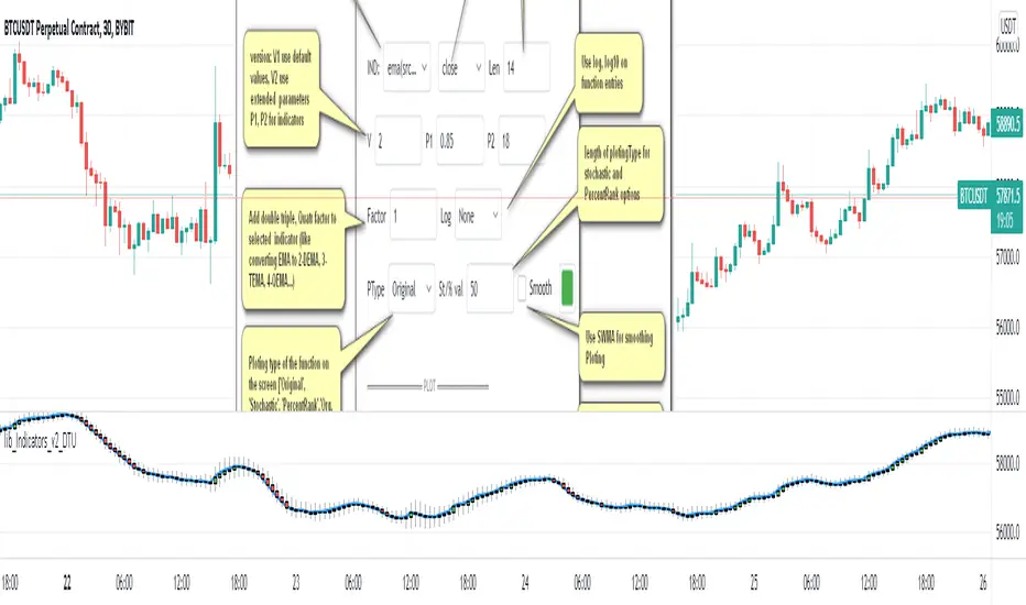
lib_Indicators_v2_DTULibrary "lib_Indicators_v2_DTU"
This library functions returns included Moving averages, indicators with factorization, functions candles, function heikinashi and more.
Created it to feed as backend of my indicator/strategy "Indicators & Combinations Framework Advanced v2 " that will be released ASAP.
This is replacement of my previous indicator (lib_indicators_DT)
I will add an indicator example which will use this indicator named as "lib_indicators_v2_DTU example" to help the usage of this library
Additionally library will be updated with more indicators in the future
NOTES:
Indicator functions returns only one series :-(
plotcandle function returns candle series
INDICATOR LIST:
hide = 'DONT DISPLAY', //Dont display & calculate the indicator. (For my framework usage)
alma = 'alma(src,len,offset=0.85,sigma=6)', //Arnaud Legoux Moving Average
ama = 'ama(src,len,fast=14,slow=100)', //Adjusted Moving Average
acdst = 'accdist()', //Accumulation/distribution index.
cma = 'cma(src,len)', //Corrective Moving average
dema = 'dema(src,len)', //Double EMA (Same as EMA with 2 factor)
ema = 'ema(src,len)', //Exponential Moving Average
gmma = 'gmma(src,len)', //Geometric Mean Moving Average
hghst = 'highest(src,len)', //Highest value for a given number of bars back.
hl2ma = 'hl2ma(src,len)', //higest lowest moving average
hma = 'hma(src,len)', //Hull Moving Average.
lgAdt = 'lagAdapt(src,len,perclen=5,fperc=50)', //Ehler's Adaptive Laguerre filter
lgAdV = 'lagAdaptV(src,len,perclen=5,fperc=50)', //Ehler's Adaptive Laguerre filter variation
lguer = 'laguerre(src,len)', //Ehler's Laguerre filter
lsrcp = 'lesrcp(src,len)', //lowest exponential esrcpanding moving line
lexp = 'lexp(src,len)', //lowest exponential expanding moving line
linrg = 'linreg(src,len,loffset=1)', //Linear regression
lowst = 'lowest(src,len)', //Lovest value for a given number of bars back.
pcnl = 'percntl(src,len)', //percentile nearest rank. Calculates percentile using method of Nearest Rank.
pcnli = 'percntli(src,len)', //percentile linear interpolation. Calculates percentile using method of linear interpolation between the two nearest ranks.
rema = 'rema(src,len)', //Range EMA (REMA)
rma = 'rma(src,len)', //Moving average used in RSI. It is the exponentially weighted moving average with alpha = 1 / length.
sma = 'sma(src,len)', //Smoothed Moving Average
smma = 'smma(src,len)', //Smoothed Moving Average
supr2 = 'super2(src,len)', //Ehler's super smoother, 2 pole
supr3 = 'super3(src,len)', //Ehler's super smoother, 3 pole
strnd = 'supertrend(src,len,period=3)', //Supertrend indicator
swma = 'swma(src,len)', //Sine-Weighted Moving Average
tema = 'tema(src,len)', //Triple EMA (Same as EMA with 3 factor)
tma = 'tma(src,len)', //Triangular Moving Average
vida = 'vida(src,len)', //Variable Index Dynamic Average
vwma = 'vwma(src,len)', //Volume Weigted Moving Average
wma = 'wma(src,len)', //Weigted Moving Average
angle = 'angle(src,len)', //angle of the series (Use its Input as another indicator output)
atr = 'atr(src,len)', //average true range. RMA of true range.
bbr = 'bbr(src,len,mult=1)', //bollinger %%
bbw = 'bbw(src,len,mult=2)', //Bollinger Bands Width. The Bollinger Band Width is the difference between the upper and the lower Bollinger Bands divided by the middle band.
cci = 'cci(src,len)', //commodity channel index
cctbb = 'cctbbo(src,len)', //CCT Bollinger Band Oscilator
chng = 'change(src,len)', //Difference between current value and previous, source - source .
cmo = 'cmo(src,len)', //Chande Momentum Oscillator. Calculates the difference between the sum of recent gains and the sum of recent losses and then divides the result by the sum of all price movement over the same period.
cog = 'cog(src,len)', //The cog (center of gravity) is an indicator based on statistics and the Fibonacci golden ratio.
cpcrv = 'copcurve(src,len)', //Coppock Curve. was originally developed by Edwin "Sedge" Coppock (Barron's Magazine, October 1962).
corrl = 'correl(src,len)', //Correlation coefficient. Describes the degree to which two series tend to deviate from their ta.sma values.
count = 'count(src,len)', //green avg - red avg
dev = 'dev(src,len)', //ta.dev() Measure of difference between the series and it's ta.sma
fall = 'falling(src,len)', //ta.falling() Test if the `source` series is now falling for `length` bars long. (Use its Input as another indicator output)
kcr = 'kcr(src,len,mult=2)', //Keltner Channels Range
kcw = 'kcw(src,len,mult=2)', //ta.kcw(). Keltner Channels Width. The Keltner Channels Width is the difference between the upper and the lower Keltner Channels divided by the middle channel.
macd = 'macd(src,len)', //macd
mfi = 'mfi(src,len)', //Money Flow Index
nvi = 'nvi()', //Negative Volume Index
obv = 'obv()', //On Balance Volume
pvi = 'pvi()', //Positive Volume Index
pvt = 'pvt()', //Price Volume Trend
rise = 'rising(src,len)', //ta.rising() Test if the `source` series is now rising for `length` bars long. (Use its Input as another indicator output)
roc = 'roc(src,len)', //Rate of Change
rsi = 'rsi(src,len)', //Relative strength Index
smosc = 'smi_osc(src,len,fast=5, slow=34)', //smi Oscillator
smsig = 'smi_sig(src,len,fast=5, slow=34)', //smi Signal
stdev = 'stdev(src,len)', //Standart deviation
trix = 'trix(src,len)' , //the rate of change of a triple exponentially smoothed moving average.
tsi = 'tsi(src,len)', //True Strength Index
vari = 'variance(src,len)', //ta.variance(). Variance is the expectation of the squared deviation of a series from its mean (ta.sma), and it informally measures how far a set of numbers are spread out from their mean.
wilpc = 'willprc(src,len)', //Williams %R
wad = 'wad()', //Williams Accumulation/Distribution.
wvad = 'wvad()' //Williams Variable Accumulation/Distribution.
}
f_func(string, float, simple, float, float, float, simple) f_func Return selected indicator value with different parameters. New version. Use extra parameters for available indicators
Parameters:
string : FuncType_ indicator from the indicator list
float : src_ close, open, high, low,hl2, hlc3, ohlc4 or any
simple : int length_ indicator length
float : p1 extra parameter-1. active on Version 2 for defining multi arguments indicator input value. ex: lagAdapt(src_, length_,LAPercLen_=p1,FPerc_=p2)
float : p2 extra parameter-2. active on Version 2 for defining multi arguments indicator input value. ex: lagAdapt(src_, length_,LAPercLen_=p1,FPerc_=p2)
float : p3 extra parameter-3. active on Version 2 for defining multi arguments indicator input value. ex: lagAdapt(src_, length_,LAPercLen_=p1,FPerc_=p2)
simple : int version_ indicator version for backward compatibility. V1:dont use extra parameters p1,p2,p3 and use default values. V2: use extra parameters for available indicators
Returns: float Return calculated indicator value
fn_heikin(float, float, float, float) fn_heikin Return given src data (open, high,low,close) as heikin ashi candle values
Parameters:
float : o_ open value
float : h_ high value
float : l_ low value
float : c_ close value
Returns: float heikin ashi open, high,low,close vlues that will be used with plotcandle
fn_plotFunction(float, string, simple, bool) fn_plotFunction Return input src data with different plotting options
Parameters:
float : src_ indicator src_data or any other series.....
string : plotingType Ploting type of the function on the screen
simple : int stochlen_ length for plotingType for stochastic and PercentRank options
bool : plotSWMA Use SWMA for smoothing Ploting
Returns: float
fn_funcPlotV2(string, float, simple, float, float, float, simple, string, simple, bool, bool) fn_funcPlotV2 Return selected indicator value with different parameters. New version. Use extra parameters fora available indicators
Parameters:
string : FuncType_ indicator from the indicator list
float : src_data_ close, open, high, low,hl2, hlc3, ohlc4 or any
simple : int length_ indicator length
float : p1 extra parameter-1. active on Version 2 for defining multi arguments indicator input value. ex: lagAdapt(src_, length_,LAPercLen_=p1,FPerc_=p2)
float : p2 extra parameter-2. active on Version 2 for defining multi arguments indicator input value. ex: lagAdapt(src_, length_,LAPercLen_=p1,FPerc_=p2)
float : p3 extra parameter-3. active on Version 2 for defining multi arguments indicator input value. ex: lagAdapt(src_, length_,LAPercLen_=p1,FPerc_=p2)
simple : int version_ indicator version for backward compatibility. V1:dont use extra parameters p1,p2,p3 and use default values. V2: use extra parameters for available indicators
string : plotingType Ploting type of the function on the screen
simple : int stochlen_ length for plotingType for stochastic and PercentRank options
bool : plotSWMA Use SWMA for smoothing Ploting
bool : log_ Use log on function entries
Returns: float Return calculated indicator value
fn_factor(string, float, simple, float, float, float, simple, simple, string, simple, bool, bool) fn_factor Return selected indicator's factorization with given arguments
Parameters:
string : FuncType_ indicator from the indicator list
float : src_data_ close, open, high, low,hl2, hlc3, ohlc4 or any
simple : int length_ indicator length
float : p1 parameter-1. active on Version 2 for defining multi arguments indicator input value. ex: lagAdapt(src_, length_,LAPercLen_=p1,FPerc_=p2)
float : p2 parameter-2. active on Version 2 for defining multi arguments indicator input value. ex: lagAdapt(src_, length_,LAPercLen_=p1,FPerc_=p2)
float : p3 parameter-3. active on Version 2 for defining multi arguments indicator input value. ex: lagAdapt(src_, length_,LAPercLen_=p1,FPerc_=p2)
simple : int version_ indicator version for backward compatibility. V1:dont use extra parameters p1,p2,p3 and use default values. V2: use extra parameters for available indicators
simple : int fact_ Add double triple, Quatr factor to selected indicator (like converting EMA to 2-DEMA, 3-TEMA, 4-QEMA...)
string : plotingType Ploting type of the function on the screen
simple : int stochlen_ length for plotingType for stochastic and PercentRank options
bool : plotSWMA Use SWMA for smoothing Ploting
bool : log_ Use log on function entries
Returns: float Return result of the function
fn_plotCandles(string, simple, float, float, float, simple, string, simple, bool, bool, bool) fn_plotCandles Return selected indicator's candle values with different parameters also heikinashi is available
Parameters:
string : FuncType_ indicator from the indicator list
simple : int length_ indicator length
float : p1 parameter-1. active on Version 2 for defining multi arguments indicator input value. ex: lagAdapt(src_, length_,LAPercLen_=p1,FPerc_=p2)
float : p2 parameter-2. active on Version 2 for defining multi arguments indicator input value. ex: lagAdapt(src_, length_,LAPercLen_=p1,FPerc_=p2)
float : p3 parameter-3. active on Version 2 for defining multi arguments indicator input value. ex: lagAdapt(src_, length_,LAPercLen_=p1,FPerc_=p2)
simple : int version_ indicator version for backward compatibility. V1:dont use extra parameters p1,p2,p3 and use default values. V2: use extra parameters for available indicators
string : plotingType Ploting type of the function on the screen
simple : int stochlen_ length for plotingType for stochastic and PercentRank options
bool : plotSWMA Use SWMA for smoothing Ploting
bool : log_ Use log on function entries
bool : plotheikin_ Use Heikin Ashi on Plot
Returns: float
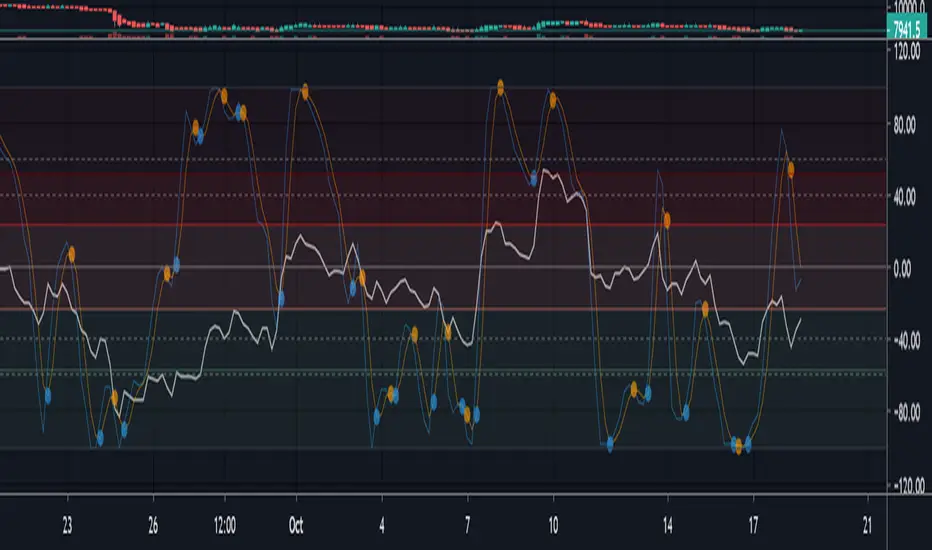
Multpile strategies [LUPOWN]///English
This indicator contains many indicators that together can form different strategies, by default there is the Latin trading strategy with the points of the cipher by @Vumanchu indicator that actually these points appear when a lazy bear indicator gives the signal, the white shadow that It is seen by default is the MFI, this adaptation is the same as the one with the indicator cipher by @Vumanchu, if the white shadow is above the 0 point we can search for a buy position, this helping us with the squeeze momentum and the ADX (information in the panel), you can even enter before the buy or sell panel if the green dot appears, this is one of several strategies that can be formed with this indicator.
Other hidden indicators by default are the CCi, Koncorde (adapted thanks to the version of @inversiones por el mundo and modified by @ lkdml), MACD, stochastic, Awesome Oscillator, Elliot Oscillator, which, as I say, combined can be good strategies.
The indicator also shows divergences, both in the RSI and in the Squeeze momentum and in the Awesome Oscillator if it is on the chart, the divergence code is from @madoqa and I adapted it for the different indicators.
The panel shows the status of the chart according to the Trading Latino strategy
You can hide and show the indicators you want through the settings.
///// Spanish
Este indicador contiene muchos indicadores que en conjunto pueden formar diversas estrategias, por default esta la estrategia de trading latino con los puntos del indicador cipher by @Vumanchu que en realidad estos puntos aparecen cuando un indicador de lazy bear da la señal, la sombra blanca que se ve por default es el MFI esta adaptación es la misma a la que tiene el indicador cipher by @Vumanchu, si la sombra blanca esta por encima del punto 0 podemos buscar entradas en compra, esto ayudándonos del squeeze momentum y el ADX (información en el panel), incluso se puede entrar antes que el panel nos de compra o venta si el punto verde aparece, esta es una de varias estrategias que se pueden formar con este indicador.
Otros indicadores ocultos por default están el CCi, Koncorde (adaptado gracias a la versión de @inversiones por el mundo y modificado por @ lkdml), MACD, estocastico , Awesome Oscillator, Elliot Oscilator, que como digo combinados se pueden hacer buenas estrategias.
En el indicador también se muestran divergencias, tanto en el RSI como en el Squeeze momentum y en el Awesome Oscillator si es que esta en el grafico, el código de divergencias es de @madoqa yo lo adapte para los diferentes indicadores.
El panel muestra el estatus del grafico según la estrategia de Trading Latino
Puedes ocultar y mostrar los indicadores que quieras mediante las configuraciones.

All in one [Liubam]Hey tradingviewers!
This is an All in one Indicator for those who can't add too many indicators on your charts. Inspired by ©LonesomeTheBlue "Indicators all in one" script. I found a lot of very interesting scripts on the public library and I decided to make a tool with some of the greatest IMO, adding some modifications to improve the indicators. With this tool you can plot 1 of 6 different indicators by selecting it from a drop-down list (on the indicator settings).
All the credit goes to it's respective owners (taggeds).
THIS INDICATOR INCLUDES:
1. Classic RSI with some OB/OS tools:
The relative strength index (RSI) is a popular momentum indicator displayed as an oscillator (a line graph that moves between two extremes) that measures the magnitude of recent price changes to evaluate overbought or oversold conditions, in other words it shows signals about bullish and bearish price momentum. I added some visual improvements to help you finding the OB/OS zones.
2. Classic CCI with some OB/OS tools.
The Commodity Channel Index (CCI) is a momentum-based oscillator used as market indicator to help determine market movements that may indicate buying or selling. Added some vistual improvements to the chart.
3. ADX and DMI oscillator with the keylevel coded by @console:
The Average Directional Index (ADX) is non-directional indicator used by some traders to determine the strength of a trend. When the ADX line is rising (Above the keylevel) trend strength is increasing, and the price moves in the direction of the trend whether up or down. Otherwise, low ADX (Below the keylevel) is usually a sign of accumulation or distribution (Range). Non-trending doesn't mean the price isn't moving. It may not be, but the price could also be making a trend change or is too volatile for a clear direction to be present.
Suggested settings of the keylevel is 23-25.... REMEMBER: The trend may be your friend.
4. MFI
The Money Flow Index (MFI) is a technical oscillator for identifying overbought or oversold signals in an asset. Unlike conventional oscillators such as the RSI, the Money Flow Index incorporates both price and volume data, as opposed to just price. It can also be used to spot divergences which warn of a trend change in price.
5. Stochastic:
A stochastic oscillator is range-bound, meaning it is always between 0 and 100. This makes it a useful indicator of overbought and oversold conditions. Traditionally, readings over 80 are considered in the overbought range, and readings under 20 are considered oversold. However, these are not always indicative of impending reversal; very strong trends can maintain overbought or oversold conditions for an extended period. Instead, traders should look to changes in the stochastic oscillator for clues about future trend shifts. I added some features for this popular indicator to show the stochastic crosses.
6. The famous Squeeze momentum Indicator made by @Lazybear:
This is derivate of John Carter's "TTM Squeeze" volatility indicator and its very strong when using with trending indicator such a ADX. Black line (or no-line) on the midline show that the market just entered a squeeze ( Bollinger Bands are with in Keltner Channel). This signifies low volatility , market preparing itself for an explosive move (up or down). Gray line signify "Squeeze release". Mr.Carter suggests waiting till the gray line after a blackline, and taking a position in the direction of the momentum (for ex., if momentum value is above zero, go long). Exit the position when the momentum changes.
------------------------------------------------------------------------------------------------------------------------------------------------------------------------------------------------------------------------------------------------
This script is source code protected, but you can add to your favorite list to use it. Also you can add twice to use 2 different indicators at the same time (E.g. Squeeze Momentum Indicator + ADX)
An additional indicator I made (MA Hunterz + InfoPanel) is needed to not miss good entry points.
Your valuable comment and feedback is much appreciated...
And remember indicators can be really helpfull but always use Price Action.
Ehlers Adaptive Commodity Channel Index V1 [CC]The Adaptive Commodity Channel Index V1 was created by John Ehlers (Rocket Science For Traders pgs 236-237) and this is the typical Commodity Channel formula with the introduction of adaptive lengths based on his earlier work with indicators such as the Mother of Adaptive Moving Averages. For longer term signals you would get a bullish signal when CCI is above 0 and a bearish signal when CCI falls below 0. For shorter term signals you would get a bullish signal when crosses over it's overbought level or when it crosses above it's oversold level or vice versa. I have included both signals to make it easier.
Let me know if you want a custom script written or if you have a special request for me

Price Action Trading System v0.3 by JustUncleL with modifcationsThe base of this script is the Price Action Trading System from JustUncle .
I have first combined it with script ADX and DI by BeikabuOyaji to indicate when the +DI is above the -DI and the ADX is above 20. This is represented by crosses at the top of the page: green indicating that the +DI is above the -DI and ADX above 20, and red if -DI is above the +DI and ADX above 20. If the ADX is increasing in slope while the +DI is above the -DI, an up green arrow is shown at the bottom of the page, indicating an increase in this trend, and the slope of the ADX is increasing and the -DI is above the +DI, a down arrow is shown at the bottom. One could think to a green cross with a green up arrow as a potential buy opportunity, and a red cross with a red down arrow as a potential sell opportunity.
Next, I have combined this script with the Indicator: WaveTrend Oscillator from Lazybear . If the oscillator has readings below -45 and the slope of the line is increasing, a green diamond appears above the chart. This indicates a potential buy opportunity. If the oscillator has readings above 50 and the slope of the line is decreasing, a red diamond appears above the chart. This indicates a potential sell opportunity. Now if the slope of the oscillator is rising significantly but does not hit the -45 threshold to start its increase, but is negative in value, a green flag appears at the top of the page. This represents a potential buy opportunity. If the slope of the oscillator is significantly decreasing and is positive in value, a red flag appears at the bottom of the page. This represents a potential sell opportunity.
The base of this script, the Price Action Trading System v0.3 by JustUncle , has many of its own features that I have kept. If the MACD is positive, the background colour is green. If it is negative, the colour is red. If the CCI and RSI indicate an oversold opportunity and the MACD is positive, you get an up olive arrow below the chart. If they indicate an overbought opportunity and the MACD is negative, you get a red down arrow above the chart. If the CCI value stays oversold after a green arrow, the candle chart turns turquoise, and if overbought, turns black after a red arrow.
You can use these indicators in combination to help you with your trading strategy.

GRAB or TrendStrength Bars with Highlights[Salty]GRAB or TrendStrength Bars with Propulsion Dots and Highlights for Squeeze Pro, CCI-Arrows, and SlowStoch
This indicator shows GRAB or TrendStrength candles and allows several moving averages to be displayed at the same time.
It has arrows and diamonds above or below the candles to show CCI values above 100 or below -100 with the arrow pointing in the direction of the momentum.
Diamonds indicate slightly weaker momentum than arrows, but still consider strong.
It has background coloring that is light green to show bullish trends and light red to show bearish trends that are derived from slow stochastics.
In general Darker colors are used for down moves and lighter colors are use to show up moves. Also, red indicates bearish, and green indicates bullish throughout.
It has yellow background to show squeezes with additional Squeeze Pro information shown at the bottom of the chart in the form of letters and momentum arrows.
L = Low compression squeeze, S = Normal Squeeze, and H = High Compression Squeeze.
It has a set of propulsion dots for each Moving Average. The trend is consider bullish when green colored dots print, and bearish when red dots print.
3 ATR Keltner channels are printed. The first two show the values used by the squeeze by default
2 Bolinger Bands are displayed based on the values used by the Squeeze by default.
1 VWAP line may be displayed.
TIP: overlaying the TICK symbol is great for confirming a bias where positive values are bullish and negative values are bearish.

Underworld Hunter Backtesting AlgorhitmThis strategy is built to prove the profitability of my Underworld Hunter indicator . It tests two different strategies. I won't be going into the calculation again since it is part of the original script. I just made a few adjustments.
First one is clearly visual. It plots slimmer twin-coloured lines now and has a different colour for every extreme level. Second is less obvious - I switched Relative Strength Index for Commodity Channel Index.
Extreme levels are as follows: green 100 -► 120, yellow 120 -► 140, orange 140 -► 160, red 160 -► 180 and purple above 180, I will have a special separate algorithm for testing optimal CCI levels someday, in this script, these values are only meant to help you with manual operations and do not influence results of the strategy in any way.
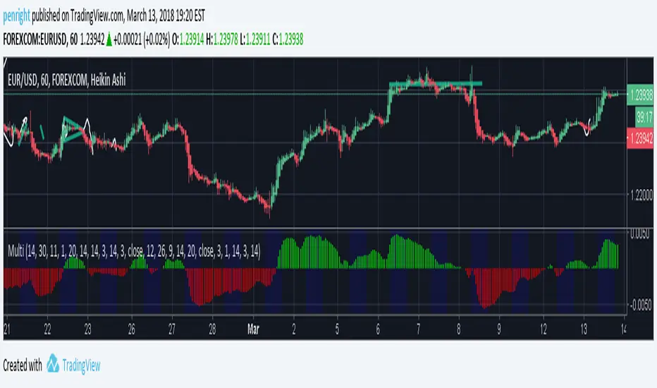
#Trending strategy
The trending strategy opens a position whenever the price leaves the bands and holds it until two consecutive bars are closed within the bands. The picture shows one winning position that hasn't yet been resulted. It also shows a few fakeouts. For this strategy, you want to keep the length below 110, the deviation should be below 2 and you probably want to play lower timeframes.
#Within the bands
The second strategy is pretty much the opposite. It opens a position when the price reaches outer bands and holds it until two consecutive bars are closed within the bands and current bar closes below previous bars low in case of long. It is working on hourly timeframes and you need higher length and deviation to succeed. The picture shows a few positions on EURUSD. Each of them is profitable but would be much higher if you closed it manually when it was time. You need to enable this strategy, which automatically disables the other one.
When using my script, you need to bear in mind that the first strategy doesn't detect optimal levels to close the price. A trend is often followed by a less volatile and boring correction which causes bands to shrink and lower your profits if you don't close manually as it will take longer till bands are reached.
On the other hand, second script literally has no stop-loss. As long as the price is outside the range, it will never close which will cause major drawdowns, unless you control the trade manually. CCI is here to help you with both.
I also recommend combining this with Market Profile (on TW, there is only Volume Profile, which can be used in a similar way) and trading day theory (trending with multiple distributions, trending day, normal day, a variation on a normal day, non-trending day or neutral day). Always keep in mind that it is up to traders to be profitable, indicators can support a good trader, but they will not fix a bad one.

Multi momentum indicatorScript contains couple momentum oscillators all in one pane
List of indicators:
RSI
Stochastic RSI
MACD
CCI
WaveTrend by LazyBear
MFI
Default active indicators are RSI and Stochastic RSI
Other indicators are disabled by default
RSI, StochRSI and MFI are modified to be bounded to range from 100 to -100. That's why overbought is 40 and 60 instead 70 and 80 while oversold -40 and -60 instead 30 and 20.
MACD and CCI as they are not bounded to 100 or 200 range, they are limited to 100 - -100 by default when activated (extras are simply hidden) but there is an option to show full indicator.
In settings there are couple more options like show crosses or show only histogram.
Default source for all indicators is close (except WaveTrend and MFI which use hlc3) and it could be changed but for all indicators.
There is an option for 2nd RSI which can be set for any timeframe and background calculated by Fibonacci levels.
cii strategy파인스크립트 공부한다고 만들어봤는데 혼자하니깐 피드백이 안되서 올려봅니다.
원리는 짧은 기간의 cci(14)가 긴 기간의 cci(56)을 뚫으면 매수, 뚫리면 매도하게 해놨습니다.
단기 분봉에는 거의 안 맞고 3시간봉 12시간봉에 맞춰서 쓰시면 됩니다. 횡보장때 승률이 많이 낮습니다..

Kringold2[WOZDUX] gold equivalentThe indicator is a tool for global analysis. The default is the price of gold. The price of the instrument from the main window is divided by the price of gold. The result is the price of the instrument in units of gold. The screen uses the Dow Jones index as an example. In the indicator window, the price of the index in units of gold or the so-called gold Dow Jones. The use of the gold equivalent makes it possible to see more truthful trends. The Indicator has the ability to change gold to any other equivalent. It is enough to change the name of the exchange and the name of the instrument in the options tool and exchange. In addition, in the settings, the second box on top allows you to view the graph in a linear or logarithmic scale. The first box at the top switches the line chart or the CCI =WT indicator to this chart.
-------------------------------------------
Индикатор это инструмент для глобального анализа. По умолчанию используется цена золота. Цена инструмента из основного окна делится на цену золота. В результате получается цена инструмента в единицах золота. На экране для примера используется индекс Доу джонса. В окне индикатора цена индекса в единицах золота или так называемый золотой Доу Джонс. Использование золотого эквивалента дает возможность видеть более правдивые тенденции движения. В Индикаторе есть возможность поменять золото на любой другой эквивалент. Достаточно в опциях инструмент и биржа изменить название биржи и название инструмента. Кроме того, в настройках, второй бокс сверху дает возможность смотреть график в линейном или логарифмическом масштабе. Первый бокс сверу переключает линейный график или индикатор CCI =WT к данному графику.

APEX - Tester - Buy/Sell Strategies - BasicThis is a simple study for backtesting your strategy for the APEX trading bot. It encorporates the following strategies and script created individually :
- Moving averages -
- Bollinger Bands -
- MACD -
- RSI -
- SRSI -
- Stochastic -
- CCI -
- Percentage Change -
- VWAP -
Be aware that the buy points will in no way be exactly the same as APEX. Some buys will be missed by apex (Spikes).
It also encorporates basic riskmangement:
TP - Take profit
SL - Stop Loss
TSL - Trailing Stop Loss
please select at minimum TP and SL combination or TSL (only TP alone wont be enough)
Additional information:
green buy triangle is the basic buy strategy
green sell is casue by TP TSL
orange sell is casue by sell strategy
orange sell is casue by sell strategy
SL red line
TP green line
TSL purple
- Riskmanagement thanks to JustUncleL
- Added S/R lines thanks to buydipsonly ( blue and yellow line )

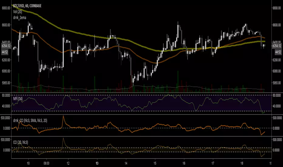
drnk_CCIClassical CCI gives the mean deviation of typical price ((high+low+close)/3) value to the simple moving average of typical price
drnk_CCI is using the same mathematical formula but configuration let you choose average type to calculate the mean deviation.
Default values gives the classic CCI
Physics MACD double// Physics MACD double 12, 26 and 5, 15
// with rsi and cci rise green on bottom
// with macd 15 rising above 0 with macd 26 below 0 green on top
// with macd 15 below 0 and macd 26 above 0 red on top
// CCI low and increasing lime bottom
// low and high volume change red green bottom circle
// use with Physics Bollinger Bands

CCI_three_timeframesThis script shows three CCIs in one frame, three different frames (20,140,3360) on the same chart.
Purely for for visual purposes values multiplied with e.
CCI is using simple moving average and mean deviation, a basic versatile momentum oscillator-indicator.
Useful for 2h charts.

A Multi 10 indicatorREAD NOTE BEFORE APPLYING or you may think indicator doesnt work.
This indicator is a revise of another i made and contains 10 Optional Indicators allowing you to load more then 3 indicators at once if you so choose and dont pay for the platform!
Hopefully someone will find use for this script besides me :) I dont suggest turning all on at once because it
will not look right. Alot will overlap if you wish but i only use the Session and trend bar at once in
conjuction with a Oscillator setting like MacD , RSI , Stoch , Aroon or CCI .
In the chart you see i only have a few indicators active ENJOY!!
---------- NOTE ----------- ( Everything is OFF by default and indicator SHOULD show up BLANK when loaded) ------------ NOTE -------------
(Can turn EVERYTHING on AND change any values in the format tab once indicator loads)
Indicators included are listed below
Sessions, including, NY session, Aussie session, Asian session, and Europe market sessions.
MacD Split Colored , aroon oscillator
CCI Oscillator , classic aroon
RSI Oscillator , Elliot wave
Stoch RSI Oscillator , ATR%
My own Trend bar
---------- NOTE ----------- ( Everything is OFF by default and indicator SHOULD show up BLANK when loaded) ------------ NOTE -------------
(Can turn EVERYTHING on AND change any values in the format tab once indicator loads) CODE probably looks messey but this is something i made for me so i didnt really care lol
A Multi 10 indicatorREAD NOTE BEFORE APPLYING or you may think indicator doesnt work.
This indicator is a revise of another i made and contains 10 Optional Indicators allowing you to load more then 3 indicators at once if you so choose and dont pay for the platform!
Hopefully someone will find use for this script besides me :) I dont suggest turning all on at once because it
will not look right. Alot will overlap if you wish but i only use the Session and trend bar at once in
conjuction with a Oscillator setting like MacD , RSI , Stoch , Aroon or CCI .
In the chart you see i only have a few indicators active ENJOY!!
---------- NOTE ----------- ( Everything is OFF by default and indicator SHOULD show up BLANK when loaded) ------------ NOTE -------------
(Can turn EVERYTHING on AND change any values in the format tab once indicator loads)
NY session, Aussie session, Asian session, and Europe market sessions.
MacD Split Colored , aroon oscillator
CCI Oscillator , classic aroon
RSI Oscillator , Elliot wave
Stoch RSI Oscillator
Aroon Oscillator
My own Trend bar
---------- NOTE ----------- ( Everything is OFF by default and indicator SHOULD show up BLANK when loaded) ------------ NOTE -------------
(Can turn EVERYTHING on AND change any values in the format tab once indicator loads) CODE probably looks messey but this is something i made for me so i didnt really care lol

TKE INDICATOR by KıvanÇ fr3762TKE INDICATOR is created by Dr Yasar ERDINC (@yerdinc65 on twitter )
It's exactly the arithmetical mean of 7 most commonly used oscillators which are:
RSI
STOCHASTIC
ULTIMATE OSCILLATOR
MFI
WIILIAMS %R
MOMENTUM
CCI
the calculation is simple:
TKE=(RSI+STOCHASTIC+ULTIMATE OSCILLATOR+MFI+WIILIAMS %R+MOMENTUM+CCI)/7
Buy signal: when TKE crosses above 20 value
Oversold region: under 20 value
Overbought region: over 80 value
Another usage of TKE is with its EMA ,
You can add the EMA line of TKE in the settings menu by clicking the "Show EMA Line" button:
the default value is defined as 5 bars of EMA of the TKE line,
Go long: when TKE crosses above EMALine
Go short: when TKE crosses below EMALine

BUBD+ - Bats Ultimate Bullish Divergence DetectorBUBD checks for price divergence from oscillators across 6 different oscillators - MACD, CCI (Vol. weighted), RSI, Stochastic RSI, Money Flow and Relative Vigor index. Use it to find good entry spots for longs and also to find downtrend reversals. If this gets popular I will release a Bearish divergence indicator as well.
Please check your stock/crypto across all time frames to get a hint of any developing "Bullish" divergences.
In case you get mixed signals -
Blue - RSI
Purple - RVI
Yellow - CCI
Green - MACD
Lime light green - MFI
Orange - Stoch RSI
Dont get confused by signals appearing on top and bottom all are bullish indicators. If you see a signal go to the respective oscillator to check the developing trend.

Volume RSIThis is a script about the RSI for the Volume Trend, with this indicator we can help us to watch the force of a volume trend (not price). Some times this can help us to clarify the change of the direction.
This is a continuation of the:
Volume Spread Graph
Volume CCI
Volume Trend Oscillator
ideas, comments and suggestions (or corrections).They are always welcome

Neural Fusion ProNeural Fusion Pro
Overview
Neural Fusion Pro is a multi-factor scoring system that combines numerous technical analysis methods into a single unified score. Rather than requiring traders to monitor multiple indicators separately, this system synthesizes trend strength, momentum oscillators, volume confirmation, price structure, and price action quality into one composite reading that adapts to current market conditions.
The Scoring System
At the heart of this indicator is a weighted scoring algorithm that produces a value between -1.0 and +1.0. Positive scores indicate bullish conditions across the measured factors, while negative scores suggest bearish conditions. The magnitude of the score reflects the strength of conviction across indicators.
The score is calculated from five distinct components, each capturing a different aspect of market behavior. Users can adjust the weight given to each component based on their trading style and market preferences.
Component 1: Trend Strength and Direction
This component uses the Average Directional Index to measure trend strength and the Directional Movement indicators to determine trend direction. When ADX exceeds the trending threshold, indicating a directional market, the component contributes a positive score if the positive directional indicator leads, or a negative score if the negative directional indicator leads. In ranging markets where ADX is low, this component contributes minimally to avoid false trend signals.
Component 2: Multi-Factor Momentum
Rather than relying on a single oscillator, this component synthesizes readings from RSI, MACD histogram, Stochastic, CCI, and Rate of Change. Each oscillator is normalized to a common scale and weighted according to its reliability characteristics. RSI readings are compared against dynamic thresholds that adjust based on trend state, making the indicator more forgiving in uptrends and more demanding in downtrends.
The component also includes divergence detection. When price makes a higher high but RSI makes a lower high (bearish divergence), or when price makes a lower low but RSI makes a higher low (bullish divergence), the divergence score adjusts the momentum component accordingly.
Component 3: Volume Confirmation
Volume provides crucial confirmation of price movements. This component analyzes On-Balance Volume relative to its moving average and measures the slope of OBV to determine whether volume is supporting the price trend. Additionally, it monitors relative volume by comparing current volume to its recent average, adding confirmation when volume spikes accompany price movements.
Component 4: Price Structure and Volatility
This component evaluates where price sits within the dynamic bands and considers the current volatility regime. When price is near the lower band, the component contributes a bullish score, suggesting potential support. When price is near the upper band, it contributes a bearish score, suggesting potential resistance.
The volatility regime assessment uses ATR percentile ranking. Low volatility periods often precede significant moves, while extremely high volatility may indicate unsustainable conditions.
Component 5: Price Action Quality
This component examines the character of recent candles by tracking the ratio of bullish to bearish candles over a lookback period. Consistent bullish price action contributes a positive score, while consistent bearish action contributes negatively. This helps filter signals by confirming that price behavior aligns with other factors.
Dynamic Bands
The indicator plots adaptive bands around a central basis line. The basis can be configured as either a simple or exponential moving average. Band width is determined by ATR multiplied by a dynamic factor that incorporates both ADX (expanding bands in trending markets) and the Chaikin Oscillator (expanding bands during strong accumulation or distribution).
These bands serve multiple purposes: they provide visual context for price position, they define signal trigger zones, and they help identify overextended conditions.
Trend State Detection
The indicator classifies market conditions into three states that affect signal generation and threshold levels.
Strong Uptrend is identified when ADX is rising, ADX exceeds the strong trend threshold, and the positive directional indicator exceeds the negative. This state triggers the most aggressive buy settings, allowing entries on shallow pullbacks.
Downtrend is identified when the negative directional indicator exceeds positive DI and ADX confirms directional movement. This state applies the most conservative buy settings, requiring deep oversold conditions before generating buy signals.
Neutral applies when neither trend condition is met, using moderate threshold settings appropriate for range-bound or transitional markets.
Dynamic RSI Thresholds
A key innovation is the automatic adjustment of RSI thresholds based on trend state. In a strong uptrend, the buy RSI threshold might be set to 50, allowing entries when RSI merely pulls back to neutral rather than requiring oversold conditions. The sell threshold rises to 72, keeping traders in positions longer during favorable conditions.
In downtrends, the buy RSI threshold drops to 25, ensuring buys only trigger on genuine capitulation. The sell threshold drops to 64, making exits easier to trigger.
In neutral markets, traditional oversold and overbought levels apply, with buy triggers around RSI 30 and sell triggers around RSI 68.
This adaptive approach prevents the common problem of indicators that work well in one market environment but fail in others.
Dynamic Cooldown
The signal cooldown period adjusts based on trend strength. During normal conditions, a standard cooldown prevents signal clustering. When ADX exceeds the strong trend threshold and is rising, indicating a powerful trend, the cooldown period extends. This helps traders stay in winning positions longer by reducing the frequency of counter-trend signals.
Cascade Protection
The indicator includes protection mechanisms to prevent overtrading and averaging down into losing positions.
The BBWP (Bollinger Band Width Percentile) monitor tracks current volatility relative to historical levels. When BBWP exceeds a threshold, indicating a volatility spike often associated with sharp moves, all buy signals are frozen. This protects against entering during panic selloffs or blow-off tops.
The consecutive buy counter tracks how many buy signals have occurred without an intervening sell. After reaching the maximum (default 3), no additional buy signals are generated until a sell occurs. This prevents the destructive pattern of repeatedly buying a declining asset.
Both protection mechanisms are displayed in the information panel, allowing traders to understand why signals may or may not be firing.
Signal Generation
Buy signals require price to touch or penetrate the lower band, RSI to be below the dynamic threshold, and the market to be in a trending state (when that filter is enabled). Additionally, the cooldown period must have elapsed and cascade protection must not be blocking buys.
Sell signals require price to touch or penetrate the upper band, RSI to be above the dynamic threshold, and the cooldown to have elapsed.
Signal labels display the entry price, signal type (shallow dip, capitulation, extended, bounce sell, or neutral), and the current position in the consecutive buy count.
Visual Components
The indicator provides multiple layers of visual feedback.
Cloud shading between the bands changes based on whether the composite score is in a buy zone or sell zone. Green clouds indicate bullish score readings, while red clouds indicate bearish readings.
Background coloring reflects the overall market regime. Green background indicates a bullish regime (positive DI leadership with volume confirmation), red indicates bearish regime, and white indicates neutral conditions.
An ADX bar at the bottom of the chart uses color coding: white for ranging (very low ADX), orange for flat, and blue for trending conditions.
The information panel displays the composite score with color coding, current trend state, active RSI thresholds, divergence status, BBWP freeze status, buy counter, market regime, ADX value with trend indicator, current cooldown setting, and live RSI reading color-coded against the active thresholds.
A debug panel can be enabled to show the individual component scores, helping users understand what is driving the composite reading.
How to Use
Monitor the composite score in the information panel. Readings above the buy threshold combined with price near the lower band represent potential long entries. Readings below the sell threshold with price near the upper band suggest exit opportunities.
Pay attention to the trend state. In strong uptrends, be more willing to buy dips and more patient with holding positions. In downtrends, require stronger confirmation before entering and be quicker to take profits on bounces.
Watch the cascade protection status. If BBWP shows frozen or the buy counter is approaching maximum, exercise additional caution regardless of other signals.
Use the dynamic RSI thresholds as context. When the panel shows buy RSI threshold at 50 (strong uptrend), even a pullback to RSI 45 is a potential entry. When the threshold shows 25 (downtrend), wait for genuine capitulation conditions.
Component Weight Adjustment
The relative importance of each scoring component can be adjusted through the settings. The default weights emphasize trend strength (30%) and momentum (25%), with volume (20%), price structure (15%), and price action (10%) providing confirmation.
For trend-following strategies, consider increasing trend and momentum weights. For mean-reversion approaches, increase the price structure weight to emphasize band position. The weights should sum to approximately 1.0 for proper score scaling.
Settings Guidance
The default settings are calibrated for cryptocurrency markets on lower timeframes. For traditional markets or longer timeframes, consider adjusting the ADX trending threshold (lower values for less volatile assets), the dynamic RSI levels for each trend state, and the cascade protection parameters.
The Heikin Ashi option for band calculation can provide smoother bands but may introduce slight lag. The default setting uses standard price data for better real-time accuracy.

5MA+TrendMagic + Disparity Scalping (SIMPLE FILTER)5MA + Trend Filter + Disparity Scalping
This multi-purpose indicator combines a five-EMA trend structure, a volatility-based trend filter, and an ultra-fast scalping module to detect both trend continuation and sharp reversal opportunities.
It is suitable for scalping, day trading, and trend-following strategies.
🔹 Main Components
1️⃣ Five-EMA Trend Structure
Displays 9 / 20 / 50 / 100 / 200 EMA levels
Helps identify short-term and long-term market direction
Useful for support and resistance during trending markets
2️⃣ Volatility-Driven Trend Filter
Uses CCI and ATR to form a dynamic trailing line
The line switches color based on momentum direction
Can act as a trailing stop or trend confirmation filter
Helps avoid counter-trend entries
3️⃣ High-Volatility GOLD Signal
Detects sudden volatility expansions using ATR, Bollinger metrics, and volatility comparison (HV vs RV)
Marks rapid breakout situations with potential continuation setups
Available for all assets, optimized for highly volatile markets
4️⃣ Ultra-Fast Disparity Scalper
Measures price deviation from EMA5 and EMA10
Confirms exhaustion using RSI + momentum prediction from a custom RVI model
Generates early BUY/SELL reversal markers
Detects momentum shifts before price fully reacts
5️⃣ Simple Overheat Filter
Prevents trades in extremely overbought/oversold zones
Gray-colored signals indicate unsafe trades to avoid
🎯 Best Use Cases
Catching early reversals during fast movement
Identifying strong trend continuation after volatility expansion
Avoiding low-probability scalps in overheated conditions
Applying EMA structure for confluence with price action
⚠️ Note
This indicator is a decision-support tool, not a standalone signal generator.
For best precision, combine with:
Market structure
Volume analysis
Support / resistance levels
🏷️ Short Description (for compact field)
Multi-function tool combining 5EMA structure, volatility-based trend filtering, and ultra-fast reversal scalping using RSI + custom RVI momentum. Ideal for both trend continuation and rapid reversals.