Sidereal Moon Cycle - NQ Special
Here is the simple breakdown of the three things you’ll see on your chart:
1. The Quarterly Backgrounds (The Big Picture)
The chart color tells you exactly where you are in the 2026 trading year. Institutions often change their "playbook" when these seasons shift.
Blue (Q1): January – March 19
Green (Q2): March 20 – June 20
Orange (Q3): June 21 – September 21
Red (Q4): September 22 – December 31
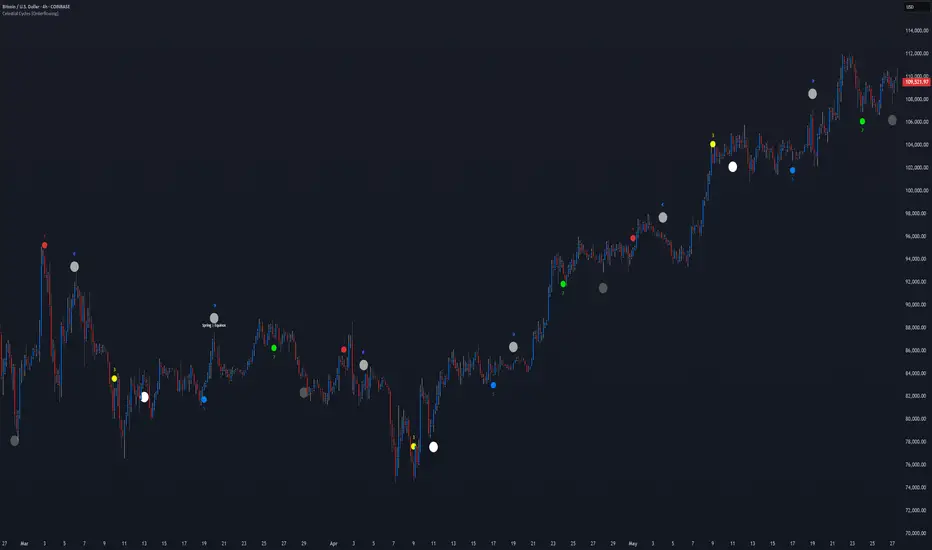
2. Gray Dashed Lines (Sidereal Cycles)
These are your Major Turning Points. They happen every 27.3 days (the time it takes the moon to return to the same spot among the stars).
What they mean: These lines represent "Energy Shifts." If NQ has been trending hard in one direction, expect it to stall, reverse, or explode when it hits a Gray Line.
How to use them: Treat these as "Time Support and Resistance." If you are in a profit, these lines are great places to take some off the table.
3. Yellow Dotted Lines (Luna Highs)
This is the "NQ PM Distortion" tracker. It’s based on the fact that the moon’s influence on the day shifts by about 50.5 minutes every single day.
The Visual: Vertical yellow dotted lines labeled "LUNA HIGH."
The Rule: These lines often pinpoint the exact 1-minute or 5-minute candle where a local high or low is formed during the New York afternoon.
How to use them: When price hits a yellow line, look for your CSID (Aqua/White) momentum signals. If they line up, you have "Time & Momentum" on your side.
4. Step-By-Step: How to Trade This
Phase Action What to look for
Preparation Identify the Quarter Are we in the Blue (Q1) or Green (Q2) season?
Anticipation Watch the Lines Is price approaching a Gray Line (Major) or a Yellow Line (Minor)?
Confirmation Wait for Price When price hits the line, does a CSID signal appear?
Execution The Entry Enter on the Retest of the level at that specific time.
The "Golden Rule" for this Script
These lines are not "Buy/Sell" buttons—they are Appointments. Think of it like this: The script tells you when the bus is arriving at the station. You still need to make sure the bus (Price) is actually stopping before you jump on.
Indicatore Pine Script®