Periodic CycleAllows visualizing a periodic cycle based on startdate, cycle period and part of cycle to be highlighed.Indicatore Pine Script®di estyles_tvr151
Bitcoin Halving Cycle Profit (with info table)English Indicator Description: Based on the original indicator by @KevinSvenson_ A table with dates was added for study purposes, however the resulting dates are not validated. The Halving Cycle Profit indicator represents a fixed, recurring profit-taking cycle that begins with each Bitcoin halving event. Functionality Explained: After every halving event, there has historically been a fixed number of weeks that marked the area of highest profitability for taking profits. • 40 weeks post-halving = Start of the optimal profit-taking zone. • 80 weeks post-halving = “Last call” for profit-taking before the bear market. • 135 weeks post-halving = Optimal area to begin Dollar-Cost Averaging (DCA). Indicatore Pine Script®di WhaleScout26
Economic Cycle ScoreCalculation -Combine Business Cycle with Liquidity Cycle by applying Z-Score -Rescale Z-Score to 0-100 -Smooth it with ema -0-15 is oversold -85-100 is overbought Use Case -Identify when risk asset (Bitcoin) is overbought/oversold -Use this indicator together with other confluences ***USE ON MONTHLY CHART ONLY (due to the economic date release frequency)Indicatore Pine Script®di MoneyPrintingCompany13
Time Cycle linesTime cycles are recurring patterns or intervals in which market movements tend to repeat. Traders use them to identify potential turning points in price action. By analyzing historical highs, lows, and key time intervals, time cycles help forecast future market behavior and improve timing for entries and exits.Indicatore Pine Script®di CasperTheTraderAggiornato 1146
Global PMI CycleGlobal business-cycle proxy derived from PMI/ISM dynamics, designed to contextualise macro regimes alongside Bitcoin and risk assets.Indicatore Pine Script®di Malcs11
Crypto Cycle Radar (TOTAL / TOTAL2 / TOTAL3 / BTC.D / USDT.D)Crypto Cycle Radar (TOTAL / TOTAL2 / TOTAL3 / BTC.D / USDT.D)Indicatore Pine Script®di nickrick1087
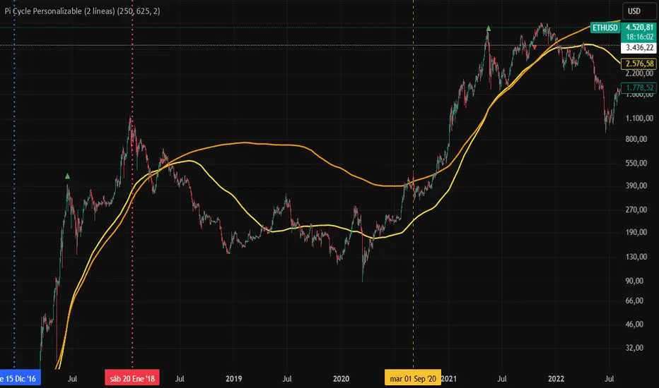
Pi Cycle PersonalizadoYou can adjust it for any crypto asset to help identify each cycle’s peaks. Example: Cardano → Fast SMA: 150 Slow SMA: 350 Ethereum → Fast SMA: 250 Slow SMA: 625Indicatore Pine Script®di fernandoriv2
Gronk-Style Lunar Cycle Projection (fixed 30m base)Based on the lunar cycle timing provided by Gronko Polo - A Bromance in FinanceIndicatore Pine Script®di ledgineer18
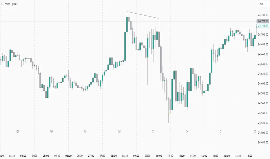
Quarterly Theory - 90m Cycles This Indicator Give you the Exact 90 mins cycles for the market and add background colors to each session over it.Indicatore Pine Script®di gbgb1bgbg122
Market Time Cycle (Expo)█ Time Cycles Overview Time cycles are a fascinating and powerful concept in the world of trading and investing. They are all about understanding and predicting the timing of market moves based on the premise that market events and price movements are not random, but instead occur in repeatable, cyclical patterns. The Concept of Time Cycles: The foundation of time cycles lies in the belief that historical market patterns tend to repeat themselves over specific periods. These periods or cycles could be influenced by a myriad of factors like economic data releases, earnings reports, geopolitical events, or even natural human behavior. For example, some traders observe increased market activity around the start and end of a trading day, which is a form of intraday time cycle. Understanding time cycles can provide traders with a roadmap, helping them anticipate potential trend shifts and make more informed decisions about when to buy or sell. █ Indicator Overview The Market Time Cycle (Expo) is designed to help traders track and analyze market cycles and generate signals for potential trading opportunities. It uses mathematical techniques to analyze market cycles and detect possible turning points. It does this by projecting the estimated cycle timeline and providing visual indications of cyclical phases through the use of color-coded lines and sine wave cycles. Time cycles offer a compelling way to forecast market trends and time your trades better. By adding time cycles to your trading toolbox, you could potentially gain a new perspective on market movements and refine your trading strategy further. The indicator generates trading signals based on the sine wave's behavior. When the sine wave crosses certain thresholds, the indicator generates a signal suggesting a potential trading opportunity based on cycle behavior. █ How to use This indicator can be a valuable tool to help traders understand and predict market trends and time their trades more accurately. By visualizing the cyclic nature of markets, traders can better anticipate potential turning points and adjust their trading strategies accordingly. It helps traders to spot ideal entry and exit points based on the cyclical nature of financial markets. █ Settings You can customize the number of bars (NumbOfBars) that are taken into consideration for the cycle. Including a higher number of bars will provide more data, which can be helpful for analyzing long-term trends. ----------------- Disclaimer The information contained in my Scripts/Indicators/Ideas/Algos/Systems does not constitute financial advice or a solicitation to buy or sell any securities of any type. I will not accept liability for any loss or damage, including without limitation any loss of profit, which may arise directly or indirectly from the use of or reliance on such information. All investments involve risk, and the past performance of a security, industry, sector, market, financial product, trading strategy, backtest, or individual's trading does not guarantee future results or returns. Investors are fully responsible for any investment decisions they make. Such decisions should be based solely on an evaluation of their financial circumstances, investment objectives, risk tolerance, and liquidity needs. My Scripts/Indicators/Ideas/Algos/Systems are only for educational purposes! Indicatore Pine Script®di Zeiierman1111 1.1 K
Goertzel Cycle Composite Wave [Loxx]As the financial markets become increasingly complex and data-driven, traders and analysts must leverage powerful tools to gain insights and make informed decisions. One such tool is the Goertzel Cycle Composite Wave indicator, a sophisticated technical analysis indicator that helps identify cyclical patterns in financial data. This powerful tool is capable of detecting cyclical patterns in financial data, helping traders to make better predictions and optimize their trading strategies. With its unique combination of mathematical algorithms and advanced charting capabilities, this indicator has the potential to revolutionize the way we approach financial modeling and trading. *** To decrease the load time of this indicator, only XX many bars back will render to the chart. You can control this value with the setting "Number of Bars to Render". This doesn't have anything to do with repainting or the indicator being endpointed*** █ Brief Overview of the Goertzel Cycle Composite Wave The Goertzel Cycle Composite Wave is a sophisticated technical analysis tool that utilizes the Goertzel algorithm to analyze and visualize cyclical components within a financial time series. By identifying these cycles and their characteristics, the indicator aims to provide valuable insights into the market's underlying price movements, which could potentially be used for making informed trading decisions. The Goertzel Cycle Composite Wave is considered a non-repainting and endpointed indicator. This means that once a value has been calculated for a specific bar, that value will not change in subsequent bars, and the indicator is designed to have a clear start and end point. This is an important characteristic for indicators used in technical analysis, as it allows traders to make informed decisions based on historical data without the risk of hindsight bias or future changes in the indicator's values. This means traders can use this indicator trading purposes. The repainting version of this indicator with forecasting, cycle selection/elimination options, and data output table can be found here: Goertzel Browser The primary purpose of this indicator is to: 1. Detect and analyze the dominant cycles present in the price data. 2. Reconstruct and visualize the composite wave based on the detected cycles. To achieve this, the indicator performs several tasks: 1. Detrending the price data: The indicator preprocesses the price data using various detrending techniques, such as Hodrick-Prescott filters, zero-lag moving averages, and linear regression, to remove the underlying trend and focus on the cyclical components. 2. Applying the Goertzel algorithm: The indicator applies the Goertzel algorithm to the detrended price data, identifying the dominant cycles and their characteristics, such as amplitude, phase, and cycle strength. 3. Constructing the composite wave: The indicator reconstructs the composite wave by combining the detected cycles, either by using a user-defined list of cycles or by selecting the top N cycles based on their amplitude or cycle strength. 4. Visualizing the composite wave: The indicator plots the composite wave, using solid lines for the cycles. The color of the lines indicates whether the wave is increasing or decreasing. This indicator is a powerful tool that employs the Goertzel algorithm to analyze and visualize the cyclical components within a financial time series. By providing insights into the underlying price movements, the indicator aims to assist traders in making more informed decisions. █ What is the Goertzel Algorithm? The Goertzel algorithm, named after Gerald Goertzel, is a digital signal processing technique that is used to efficiently compute individual terms of the Discrete Fourier Transform (DFT). It was first introduced in 1958, and since then, it has found various applications in the fields of engineering, mathematics, and physics. The Goertzel algorithm is primarily used to detect specific frequency components within a digital signal, making it particularly useful in applications where only a few frequency components are of interest. The algorithm is computationally efficient, as it requires fewer calculations than the Fast Fourier Transform (FFT) when detecting a small number of frequency components. This efficiency makes the Goertzel algorithm a popular choice in applications such as: 1. Telecommunications: The Goertzel algorithm is used for decoding Dual-Tone Multi-Frequency (DTMF) signals, which are the tones generated when pressing buttons on a telephone keypad. By identifying specific frequency components, the algorithm can accurately determine which button has been pressed. 2. Audio processing: The algorithm can be used to detect specific pitches or harmonics in an audio signal, making it useful in applications like pitch detection and tuning musical instruments. 3. Vibration analysis: In the field of mechanical engineering, the Goertzel algorithm can be applied to analyze vibrations in rotating machinery, helping to identify faulty components or signs of wear. 4. Power system analysis: The algorithm can be used to measure harmonic content in power systems, allowing engineers to assess power quality and detect potential issues. The Goertzel algorithm is used in these applications because it offers several advantages over other methods, such as the FFT: 1. Computational efficiency: The Goertzel algorithm requires fewer calculations when detecting a small number of frequency components, making it more computationally efficient than the FFT in these cases. 2. Real-time analysis: The algorithm can be implemented in a streaming fashion, allowing for real-time analysis of signals, which is crucial in applications like telecommunications and audio processing. 3. Memory efficiency: The Goertzel algorithm requires less memory than the FFT, as it only computes the frequency components of interest. 4. Precision: The algorithm is less susceptible to numerical errors compared to the FFT, ensuring more accurate results in applications where precision is essential. The Goertzel algorithm is an efficient digital signal processing technique that is primarily used to detect specific frequency components within a signal. Its computational efficiency, real-time capabilities, and precision make it an attractive choice for various applications, including telecommunications, audio processing, vibration analysis, and power system analysis. The algorithm has been widely adopted since its introduction in 1958 and continues to be an essential tool in the fields of engineering, mathematics, and physics. █ Goertzel Algorithm in Quantitative Finance: In-Depth Analysis and Applications The Goertzel algorithm, initially designed for signal processing in telecommunications, has gained significant traction in the financial industry due to its efficient frequency detection capabilities. In quantitative finance, the Goertzel algorithm has been utilized for uncovering hidden market cycles, developing data-driven trading strategies, and optimizing risk management. This section delves deeper into the applications of the Goertzel algorithm in finance, particularly within the context of quantitative trading and analysis. Unveiling Hidden Market Cycles: Market cycles are prevalent in financial markets and arise from various factors, such as economic conditions, investor psychology, and market participant behavior. The Goertzel algorithm's ability to detect and isolate specific frequencies in price data helps trader analysts identify hidden market cycles that may otherwise go unnoticed. By examining the amplitude, phase, and periodicity of each cycle, traders can better understand the underlying market structure and dynamics, enabling them to develop more informed and effective trading strategies. Developing Quantitative Trading Strategies: The Goertzel algorithm's versatility allows traders to incorporate its insights into a wide range of trading strategies. By identifying the dominant market cycles in a financial instrument's price data, traders can create data-driven strategies that capitalize on the cyclical nature of markets. For instance, a trader may develop a mean-reversion strategy that takes advantage of the identified cycles. By establishing positions when the price deviates from the predicted cycle, the trader can profit from the subsequent reversion to the cycle's mean. Similarly, a momentum-based strategy could be designed to exploit the persistence of a dominant cycle by entering positions that align with the cycle's direction. Enhancing Risk Management: The Goertzel algorithm plays a vital role in risk management for quantitative strategies. By analyzing the cyclical components of a financial instrument's price data, traders can gain insights into the potential risks associated with their trading strategies. By monitoring the amplitude and phase of dominant cycles, a trader can detect changes in market dynamics that may pose risks to their positions. For example, a sudden increase in amplitude may indicate heightened volatility, prompting the trader to adjust position sizing or employ hedging techniques to protect their portfolio. Additionally, changes in phase alignment could signal a potential shift in market sentiment, necessitating adjustments to the trading strategy. Expanding Quantitative Toolkits: Traders can augment the Goertzel algorithm's insights by combining it with other quantitative techniques, creating a more comprehensive and sophisticated analysis framework. For example, machine learning algorithms, such as neural networks or support vector machines, could be trained on features extracted from the Goertzel algorithm to predict future price movements more accurately. Furthermore, the Goertzel algorithm can be integrated with other technical analysis tools, such as moving averages or oscillators, to enhance their effectiveness. By applying these tools to the identified cycles, traders can generate more robust and reliable trading signals. The Goertzel algorithm offers invaluable benefits to quantitative finance practitioners by uncovering hidden market cycles, aiding in the development of data-driven trading strategies, and improving risk management. By leveraging the insights provided by the Goertzel algorithm and integrating it with other quantitative techniques, traders can gain a deeper understanding of market dynamics and devise more effective trading strategies. █ Indicator Inputs src: This is the source data for the analysis, typically the closing price of the financial instrument. detrendornot: This input determines the method used for detrending the source data. Detrending is the process of removing the underlying trend from the data to focus on the cyclical components. The available options are: hpsmthdt: Detrend using Hodrick-Prescott filter centered moving average. zlagsmthdt: Detrend using zero-lag moving average centered moving average. logZlagRegression: Detrend using logarithmic zero-lag linear regression. hpsmth: Detrend using Hodrick-Prescott filter. zlagsmth: Detrend using zero-lag moving average. DT_HPper1 and DT_HPper2: These inputs define the period range for the Hodrick-Prescott filter centered moving average when detrendornot is set to hpsmthdt. DT_ZLper1 and DT_ZLper2: These inputs define the period range for the zero-lag moving average centered moving average when detrendornot is set to zlagsmthdt. DT_RegZLsmoothPer: This input defines the period for the zero-lag moving average used in logarithmic zero-lag linear regression when detrendornot is set to logZlagRegression. HPsmoothPer: This input defines the period for the Hodrick-Prescott filter when detrendornot is set to hpsmth. ZLMAsmoothPer: This input defines the period for the zero-lag moving average when detrendornot is set to zlagsmth. MaxPer: This input sets the maximum period for the Goertzel algorithm to search for cycles. squaredAmp: This boolean input determines whether the amplitude should be squared in the Goertzel algorithm. useAddition: This boolean input determines whether the Goertzel algorithm should use addition for combining the cycles. useCosine: This boolean input determines whether the Goertzel algorithm should use cosine waves instead of sine waves. UseCycleStrength: This boolean input determines whether the Goertzel algorithm should compute the cycle strength, which is a normalized measure of the cycle's amplitude. WindowSizePast: These inputs define the window size for the composite wave. FilterBartels: This boolean input determines whether Bartel's test should be applied to filter out non-significant cycles. BartNoCycles: This input sets the number of cycles to be used in Bartel's test. BartSmoothPer: This input sets the period for the moving average used in Bartel's test. BartSigLimit: This input sets the significance limit for Bartel's test, below which cycles are considered insignificant. SortBartels: This boolean input determines whether the cycles should be sorted by their Bartel's test results. StartAtCycle: This input determines the starting index for selecting the top N cycles when UseCycleList is set to false. This allows you to skip a certain number of cycles from the top before selecting the desired number of cycles. UseTopCycles: This input sets the number of top cycles to use for constructing the composite wave when UseCycleList is set to false. The cycles are ranked based on their amplitudes or cycle strengths, depending on the UseCycleStrength input. SubtractNoise: This boolean input determines whether to subtract the noise (remaining cycles) from the composite wave. If set to true, the composite wave will only include the top N cycles specified by UseTopCycles. █ Exploring Auxiliary Functions The following functions demonstrate advanced techniques for analyzing financial markets, including zero-lag moving averages, Bartels probability, detrending, and Hodrick-Prescott filtering. This section examines each function in detail, explaining their purpose, methodology, and applications in finance. We will examine how each function contributes to the overall performance and effectiveness of the indicator and how they work together to create a powerful analytical tool. Zero-Lag Moving Average: The zero-lag moving average function is designed to minimize the lag typically associated with moving averages. This is achieved through a two-step weighted linear regression process that emphasizes more recent data points. The function calculates a linearly weighted moving average (LWMA) on the input data and then applies another LWMA on the result. By doing this, the function creates a moving average that closely follows the price action, reducing the lag and improving the responsiveness of the indicator. The zero-lag moving average function is used in the indicator to provide a responsive, low-lag smoothing of the input data. This function helps reduce the noise and fluctuations in the data, making it easier to identify and analyze underlying trends and patterns. By minimizing the lag associated with traditional moving averages, this function allows the indicator to react more quickly to changes in market conditions, providing timely signals and improving the overall effectiveness of the indicator. Bartels Probability: The Bartels probability function calculates the probability of a given cycle being significant in a time series. It uses a mathematical test called the Bartels test to assess the significance of cycles detected in the data. The function calculates coefficients for each detected cycle and computes an average amplitude and an expected amplitude. By comparing these values, the Bartels probability is derived, indicating the likelihood of a cycle's significance. This information can help in identifying and analyzing dominant cycles in financial markets. The Bartels probability function is incorporated into the indicator to assess the significance of detected cycles in the input data. By calculating the Bartels probability for each cycle, the indicator can prioritize the most significant cycles and focus on the market dynamics that are most relevant to the current trading environment. This function enhances the indicator's ability to identify dominant market cycles, improving its predictive power and aiding in the development of effective trading strategies. Detrend Logarithmic Zero-Lag Regression: The detrend logarithmic zero-lag regression function is used for detrending data while minimizing lag. It combines a zero-lag moving average with a linear regression detrending method. The function first calculates the zero-lag moving average of the logarithm of input data and then applies a linear regression to remove the trend. By detrending the data, the function isolates the cyclical components, making it easier to analyze and interpret the underlying market dynamics. The detrend logarithmic zero-lag regression function is used in the indicator to isolate the cyclical components of the input data. By detrending the data, the function enables the indicator to focus on the cyclical movements in the market, making it easier to analyze and interpret market dynamics. This function is essential for identifying cyclical patterns and understanding the interactions between different market cycles, which can inform trading decisions and enhance overall market understanding. Bartels Cycle Significance Test: The Bartels cycle significance test is a function that combines the Bartels probability function and the detrend logarithmic zero-lag regression function to assess the significance of detected cycles. The function calculates the Bartels probability for each cycle and stores the results in an array. By analyzing the probability values, traders and analysts can identify the most significant cycles in the data, which can be used to develop trading strategies and improve market understanding. The Bartels cycle significance test function is integrated into the indicator to provide a comprehensive analysis of the significance of detected cycles. By combining the Bartels probability function and the detrend logarithmic zero-lag regression function, this test evaluates the significance of each cycle and stores the results in an array. The indicator can then use this information to prioritize the most significant cycles and focus on the most relevant market dynamics. This function enhances the indicator's ability to identify and analyze dominant market cycles, providing valuable insights for trading and market analysis. Hodrick-Prescott Filter: The Hodrick-Prescott filter is a popular technique used to separate the trend and cyclical components of a time series. The function applies a smoothing parameter to the input data and calculates a smoothed series using a two-sided filter. This smoothed series represents the trend component, which can be subtracted from the original data to obtain the cyclical component. The Hodrick-Prescott filter is commonly used in economics and finance to analyze economic data and financial market trends. The Hodrick-Prescott filter is incorporated into the indicator to separate the trend and cyclical components of the input data. By applying the filter to the data, the indicator can isolate the trend component, which can be used to analyze long-term market trends and inform trading decisions. Additionally, the cyclical component can be used to identify shorter-term market dynamics and provide insights into potential trading opportunities. The inclusion of the Hodrick-Prescott filter adds another layer of analysis to the indicator, making it more versatile and comprehensive. Detrending Options: Detrend Centered Moving Average: The detrend centered moving average function provides different detrending methods, including the Hodrick-Prescott filter and the zero-lag moving average, based on the selected detrending method. The function calculates two sets of smoothed values using the chosen method and subtracts one set from the other to obtain a detrended series. By offering multiple detrending options, this function allows traders and analysts to select the most appropriate method for their specific needs and preferences. The detrend centered moving average function is integrated into the indicator to provide users with multiple detrending options, including the Hodrick-Prescott filter and the zero-lag moving average. By offering multiple detrending methods, the indicator allows users to customize the analysis to their specific needs and preferences, enhancing the indicator's overall utility and adaptability. This function ensures that the indicator can cater to a wide range of trading styles and objectives, making it a valuable tool for a diverse group of market participants. The auxiliary functions functions discussed in this section demonstrate the power and versatility of mathematical techniques in analyzing financial markets. By understanding and implementing these functions, traders and analysts can gain valuable insights into market dynamics, improve their trading strategies, and make more informed decisions. The combination of zero-lag moving averages, Bartels probability, detrending methods, and the Hodrick-Prescott filter provides a comprehensive toolkit for analyzing and interpreting financial data. The integration of advanced functions in a financial indicator creates a powerful and versatile analytical tool that can provide valuable insights into financial markets. By combining the zero-lag moving average, █ In-Depth Analysis of the Goertzel Cycle Composite Wave Code The Goertzel Cycle Composite Wave code is an implementation of the Goertzel Algorithm, an efficient technique to perform spectral analysis on a signal. The code is designed to detect and analyze dominant cycles within a given financial market data set. This section will provide an extremely detailed explanation of the code, its structure, functions, and intended purpose. Function signature and input parameters: The Goertzel Cycle Composite Wave function accepts numerous input parameters for customization, including source data (src), the current bar (forBar), sample size (samplesize), period (per), squared amplitude flag (squaredAmp), addition flag (useAddition), cosine flag (useCosine), cycle strength flag (UseCycleStrength), past sizes (WindowSizePast), Bartels filter flag (FilterBartels), Bartels-related parameters (BartNoCycles, BartSmoothPer, BartSigLimit), sorting flag (SortBartels), and output buffers (goeWorkPast, cyclebuffer, amplitudebuffer, phasebuffer, cycleBartelsBuffer). Initializing variables and arrays: The code initializes several float arrays (goeWork1, goeWork2, goeWork3, goeWork4) with the same length as twice the period (2 * per). These arrays store intermediate results during the execution of the algorithm. Preprocessing input data: The input data (src) undergoes preprocessing to remove linear trends. This step enhances the algorithm's ability to focus on cyclical components in the data. The linear trend is calculated by finding the slope between the first and last values of the input data within the sample. Iterative calculation of Goertzel coefficients: The core of the Goertzel Cycle Composite Wave algorithm lies in the iterative calculation of Goertzel coefficients for each frequency bin. These coefficients represent the spectral content of the input data at different frequencies. The code iterates through the range of frequencies, calculating the Goertzel coefficients using a nested loop structure. Cycle strength computation: The code calculates the cycle strength based on the Goertzel coefficients. This is an optional step, controlled by the UseCycleStrength flag. The cycle strength provides information on the relative influence of each cycle on the data per bar, considering both amplitude and cycle length. The algorithm computes the cycle strength either by squaring the amplitude (controlled by squaredAmp flag) or using the actual amplitude values. Phase calculation: The Goertzel Cycle Composite Wave code computes the phase of each cycle, which represents the position of the cycle within the input data. The phase is calculated using the arctangent function (math.atan) based on the ratio of the imaginary and real components of the Goertzel coefficients. Peak detection and cycle extraction: The algorithm performs peak detection on the computed amplitudes or cycle strengths to identify dominant cycles. It stores the detected cycles in the cyclebuffer array, along with their corresponding amplitudes and phases in the amplitudebuffer and phasebuffer arrays, respectively. Sorting cycles by amplitude or cycle strength: The code sorts the detected cycles based on their amplitude or cycle strength in descending order. This allows the algorithm to prioritize cycles with the most significant impact on the input data. Bartels cycle significance test: If the FilterBartels flag is set, the code performs a Bartels cycle significance test on the detected cycles. This test determines the statistical significance of each cycle and filters out the insignificant cycles. The significant cycles are stored in the cycleBartelsBuffer array. If the SortBartels flag is set, the code sorts the significant cycles based on their Bartels significance values. Waveform calculation: The Goertzel Cycle Composite Wave code calculates the waveform of the significant cycles for specified time windows. The windows are defined by the WindowSizePast parameters, respectively. The algorithm uses either cosine or sine functions (controlled by the useCosine flag) to calculate the waveforms for each cycle. The useAddition flag determines whether the waveforms should be added or subtracted. Storing waveforms in a matrix: The calculated waveforms for the cycle is stored in the matrix - goeWorkPast. This matrix holds the waveforms for the specified time windows. Each row in the matrix represents a time window position, and each column corresponds to a cycle. Returning the number of cycles: The Goertzel Cycle Composite Wave function returns the total number of detected cycles (number_of_cycles) after processing the input data. This information can be used to further analyze the results or to visualize the detected cycles. The Goertzel Cycle Composite Wave code is a comprehensive implementation of the Goertzel Algorithm, specifically designed for detecting and analyzing dominant cycles within financial market data. The code offers a high level of customization, allowing users to fine-tune the algorithm based on their specific needs. The Goertzel Cycle Composite Wave's combination of preprocessing, iterative calculations, cycle extraction, sorting, significance testing, and waveform calculation makes it a powerful tool for understanding cyclical components in financial data. █ Generating and Visualizing Composite Waveform The indicator calculates and visualizes the composite waveform for specified time windows based on the detected cycles. Here's a detailed explanation of this process: Updating WindowSizePast: The WindowSizePast is updated to ensure they are at least twice the MaxPer (maximum period). Initializing matrices and arrays: The matrix goeWorkPast is initialized to store the Goertzel results for specified time windows. Multiple arrays are also initialized to store cycle, amplitude, phase, and Bartels information. Preparing the source data (srcVal) array: The source data is copied into an array, srcVal, and detrended using one of the selected methods (hpsmthdt, zlagsmthdt, logZlagRegression, hpsmth, or zlagsmth). Goertzel function call: The Goertzel function is called to analyze the detrended source data and extract cycle information. The output, number_of_cycles, contains the number of detected cycles. Initializing arrays for waveforms: The goertzel array is initialized to store the endpoint Goertzel. Calculating composite waveform (goertzel array): The composite waveform is calculated by summing the selected cycles (either from the user-defined cycle list or the top cycles) and optionally subtracting the noise component. Drawing composite waveform (pvlines): The composite waveform is drawn on the chart using solid lines. The color of the lines is determined by the direction of the waveform (green for upward, red for downward). To summarize, this indicator generates a composite waveform based on the detected cycles in the financial data. It calculates the composite waveforms and visualizes them on the chart using colored lines. █ Enhancing the Goertzel Algorithm-Based Script for Financial Modeling and Trading The Goertzel algorithm-based script for detecting dominant cycles in financial data is a powerful tool for financial modeling and trading. It provides valuable insights into the past behavior of these cycles. However, as with any algorithm, there is always room for improvement. This section discusses potential enhancements to the existing script to make it even more robust and versatile for financial modeling, general trading, advanced trading, and high-frequency finance trading. Enhancements for Financial Modeling Data preprocessing: One way to improve the script's performance for financial modeling is to introduce more advanced data preprocessing techniques. This could include removing outliers, handling missing data, and normalizing the data to ensure consistent and accurate results. Additional detrending and smoothing methods: Incorporating more sophisticated detrending and smoothing techniques, such as wavelet transform or empirical mode decomposition, can help improve the script's ability to accurately identify cycles and trends in the data. Machine learning integration: Integrating machine learning techniques, such as artificial neural networks or support vector machines, can help enhance the script's predictive capabilities, leading to more accurate financial models. Enhancements for General and Advanced Trading Customizable indicator integration: Allowing users to integrate their own technical indicators can help improve the script's effectiveness for both general and advanced trading. By enabling the combination of the dominant cycle information with other technical analysis tools, traders can develop more comprehensive trading strategies. Risk management and position sizing: Incorporating risk management and position sizing functionality into the script can help traders better manage their trades and control potential losses. This can be achieved by calculating the optimal position size based on the user's risk tolerance and account size. Multi-timeframe analysis: Enhancing the script to perform multi-timeframe analysis can provide traders with a more holistic view of market trends and cycles. By identifying dominant cycles on different timeframes, traders can gain insights into the potential confluence of cycles and make better-informed trading decisions. Enhancements for High-Frequency Finance Trading Algorithm optimization: To ensure the script's suitability for high-frequency finance trading, optimizing the algorithm for faster execution is crucial. This can be achieved by employing efficient data structures and refining the calculation methods to minimize computational complexity. Real-time data streaming: Integrating real-time data streaming capabilities into the script can help high-frequency traders react to market changes more quickly. By continuously updating the cycle information based on real-time market data, traders can adapt their strategies accordingly and capitalize on short-term market fluctuations. Order execution and trade management: To fully leverage the script's capabilities for high-frequency trading, implementing functionality for automated order execution and trade management is essential. This can include features such as stop-loss and take-profit orders, trailing stops, and automated trade exit strategies. While the existing Goertzel algorithm-based script is a valuable tool for detecting dominant cycles in financial data, there are several potential enhancements that can make it even more powerful for financial modeling, general trading, advanced trading, and high-frequency finance trading. By incorporating these improvements, the script can become a more versatile and effective tool for traders and financial analysts alike. █ Understanding the Limitations of the Goertzel Algorithm While the Goertzel algorithm-based script for detecting dominant cycles in financial data provides valuable insights, it is important to be aware of its limitations and drawbacks. Some of the key drawbacks of this indicator are: Lagging nature: As with many other technical indicators, the Goertzel algorithm-based script can suffer from lagging effects, meaning that it may not immediately react to real-time market changes. This lag can lead to late entries and exits, potentially resulting in reduced profitability or increased losses. Parameter sensitivity: The performance of the script can be sensitive to the chosen parameters, such as the detrending methods, smoothing techniques, and cycle detection settings. Improper parameter selection may lead to inaccurate cycle detection or increased false signals, which can negatively impact trading performance. Complexity: The Goertzel algorithm itself is relatively complex, making it difficult for novice traders or those unfamiliar with the concept of cycle analysis to fully understand and effectively utilize the script. This complexity can also make it challenging to optimize the script for specific trading styles or market conditions. Overfitting risk: As with any data-driven approach, there is a risk of overfitting when using the Goertzel algorithm-based script. Overfitting occurs when a model becomes too specific to the historical data it was trained on, leading to poor performance on new, unseen data. This can result in misleading signals and reduced trading performance. Limited applicability: The Goertzel algorithm-based script may not be suitable for all markets, trading styles, or timeframes. Its effectiveness in detecting cycles may be limited in certain market conditions, such as during periods of extreme volatility or low liquidity. While the Goertzel algorithm-based script offers valuable insights into dominant cycles in financial data, it is essential to consider its drawbacks and limitations when incorporating it into a trading strategy. Traders should always use the script in conjunction with other technical and fundamental analysis tools, as well as proper risk management, to make well-informed trading decisions. █ Interpreting Results The Goertzel Cycle Composite Wave indicator can be interpreted by analyzing the plotted lines. The indicator plots two lines: composite waves. The composite wave represents the composite wave of the price data. The composite wave line displays a solid line, with green indicating a bullish trend and red indicating a bearish trend. Interpreting the Goertzel Cycle Composite Wave indicator involves identifying the trend of the composite wave lines and matching them with the corresponding bullish or bearish color. █ Conclusion The Goertzel Cycle Composite Wave indicator is a powerful tool for identifying and analyzing cyclical patterns in financial markets. Its ability to detect multiple cycles of varying frequencies and strengths make it a valuable addition to any trader's technical analysis toolkit. However, it is important to keep in mind that the Goertzel Cycle Composite Wave indicator should be used in conjunction with other technical analysis tools and fundamental analysis to achieve the best results. With continued refinement and development, the Goertzel Cycle Composite Wave indicator has the potential to become a highly effective tool for financial modeling, general trading, advanced trading, and high-frequency finance trading. Its accuracy and versatility make it a promising candidate for further research and development. █ Footnotes What is the Bartels Test for Cycle Significance? The Bartels Cycle Significance Test is a statistical method that determines whether the peaks and troughs of a time series are statistically significant. The test is named after its inventor, George Bartels, who developed it in the mid-20th century. The Bartels test is designed to analyze the cyclical components of a time series, which can help traders and analysts identify trends and cycles in financial markets. The test calculates a Bartels statistic, which measures the degree of non-randomness or autocorrelation in the time series. The Bartels statistic is calculated by first splitting the time series into two halves and calculating the range of the peaks and troughs in each half. The test then compares these ranges using a t-test, which measures the significance of the difference between the two ranges. If the Bartels statistic is greater than a critical value, it indicates that the peaks and troughs in the time series are non-random and that there is a significant cyclical component to the data. Conversely, if the Bartels statistic is less than the critical value, it suggests that the peaks and troughs are random and that there is no significant cyclical component. The Bartels Cycle Significance Test is particularly useful in financial analysis because it can help traders and analysts identify significant cycles in asset prices, which can in turn inform investment decisions. However, it is important to note that the test is not perfect and can produce false signals in certain situations, particularly in noisy or volatile markets. Therefore, it is always recommended to use the test in conjunction with other technical and fundamental indicators to confirm trends and cycles. Deep-dive into the Hodrick-Prescott Fitler The Hodrick-Prescott (HP) filter is a statistical tool used in economics and finance to separate a time series into two components: a trend component and a cyclical component. It is a powerful tool for identifying long-term trends in economic and financial data and is widely used by economists, central banks, and financial institutions around the world. The HP filter was first introduced in the 1990s by economists Robert Hodrick and Edward Prescott. It is a simple, two-parameter filter that separates a time series into a trend component and a cyclical component. The trend component represents the long-term behavior of the data, while the cyclical component captures the shorter-term fluctuations around the trend. The HP filter works by minimizing the following objective function: Minimize: (Sum of Squared Deviations) + λ (Sum of Squared Second Differences) Where: 1. The first term represents the deviation of the data from the trend. 2. The second term represents the smoothness of the trend. 3. λ is a smoothing parameter that determines the degree of smoothness of the trend. The smoothing parameter λ is typically set to a value between 100 and 1600, depending on the frequency of the data. Higher values of λ lead to a smoother trend, while lower values lead to a more volatile trend. The HP filter has several advantages over other smoothing techniques. It is a non-parametric method, meaning that it does not make any assumptions about the underlying distribution of the data. It also allows for easy comparison of trends across different time series and can be used with data of any frequency. However, the HP filter also has some limitations. It assumes that the trend is a smooth function, which may not be the case in some situations. It can also be sensitive to changes in the smoothing parameter λ, which may result in different trends for the same data. Additionally, the filter may produce unrealistic trends for very short time series. Despite these limitations, the HP filter remains a valuable tool for analyzing economic and financial data. It is widely used by central banks and financial institutions to monitor long-term trends in the economy, and it can be used to identify turning points in the business cycle. The filter can also be used to analyze asset prices, exchange rates, and other financial variables. The Hodrick-Prescott filter is a powerful tool for analyzing economic and financial data. It separates a time series into a trend component and a cyclical component, allowing for easy identification of long-term trends and turning points in the business cycle. While it has some limitations, it remains a valuable tool for economists, central banks, and financial institutions around the world.Indicatore Pine Script®di loxx33376
SMT Cycles by AlgoKingsSMT Cycles by AlgoKings RISK DISCLAIMER: This indicator is an analytical tool for educational purposes only, not financial advice. Trading carries substantial risk of loss. This tool does not guarantee profitable trades. Always use proper risk management and never risk more than you can afford to lose. WHAT ARE SMT CYCLES? This indicator identifies Smart Money Technique divergences using cycle-based analysis rather than standard timeframes. Cycles represent natural market rhythms (sessions, 90-minute institutional windows, true daily periods) that better align with institutional trading patterns than arbitrary timeframe bars. Example: During the London session, NQ makes a new high but ES fails to follow = Bearish SMT divergence within the London cycle UNDERLYING METHODOLOGY This indicator combines four analytical layers: 1. AUTOMATIC CORRELATION MAPPING Built-in correlation intelligence for 40+ pairs (identical to SMT Custom): - Futures: NQ, ES, YM cross-correlation | GC/SI | 6E/6B - Forex: EURUSD/GBPUSD/DXY(inverse) | AUDUSD/NZDUSD - Stocks: MAG7 (META, NVDA, MSFT, etc.) vs NDX - Crypto: BTCUSD/ETHUSD Algorithm automatically mirrors contract types and exchange prefixes using regex-based parsing for futures contracts and micro variants. 2. CYCLE-BASED PERIOD DETECTION Unlike standard timeframe analysis, this indicator uses market structure cycles: SWING CYCLES (Position Trading): - Yearly: 12-month institutional rebalancing periods - Quarterly: 3-month earnings and fund rotation cycles - Monthly: Calendar month institutional flows - Weekly: 7-day swing trading cycles - Daily: Standard 18:00-18:00 EST bars - TrueDay: 00:00-00:00 EST for 24-hour markets (futures, forex, crypto) INTRADAY CYCLES (Day Trading): - Session: Asia (18:00-02:00), London (02:00-08:30), NY AM (08:30-12:00), NY PM (12:00-17:00) EST - 90m: Three 90-minute windows per trading day (02:00-03:30, 03:30-05:00, etc.) - 30m: 30-minute institutional order flow windows - 10m, 3m, 1m: Scalping cycles for precise entry timing Technical implementation: - TrueDay calculation: Detects candle closes at exactly 00:00 EST using time modulo arithmetic on 24-hour markets. Differs from standard Daily bars which use futures settlement times (18:00 EST). - Session detection: Regex pattern matching on hour/minute timestamps to identify cycle boundaries (e.g., h==2 and m==0 triggers Asia session end) - 90m hierarchy: Groups sub-90m cycles (30m, 10m, 3m, 1m) under their parent 90m window using group timestamp tracking (gx field) - Intermediate accumulation: For multi-bar cycles (TrueDay, Sessions, 90m), maintains running high/low (nh1, nl1) across constituent bars until cycle completion 3. MULTI-TIMEFRAME CYCLE ANALYSIS Proprietary cycle synchronization: - Tracks price structure across up to 11 configurable cycles simultaneously - Maintains independent high/low tracking for each symbol pair using request.security() - Compares previous cycle extremes (high , low ) across correlated pairs - Timestamps divergence formations at chart timeframe precision - Implements adaptive purge logic (1min to 12M) based on cycle type 4. DIVERGENCE CLASSIFICATION SYSTEM Bullish SMT: Chart symbol makes lower low within cycle, correlated pair does NOT = Institutional buying pressure Bearish SMT: Chart symbol makes higher high within cycle, correlated pair does NOT = Institutional selling pressure Advanced features include level tracking (monitors when extremes are revisited), automatic extension until both levels violated, 90m hierarchy overlap filtering (hides sub-90m SMT within parent 90m window), and inverse correlation support for DXY relationships. WHY CLOSED-SOURCE? This script protects proprietary algorithms: - Cycle boundary detection: Custom logic for TrueDay calculation (00:00 EST candle close detection using modulo arithmetic on 24h markets), Session identification (time-based regex for Asia/London/NY periods), and 90m window calculation (minute offset from 02:00 EST baseline) - Intermediate cycle accumulation: Complex state management for multi-bar cycles (Sessions, 90m, TrueDay) that build complete cycle values across constituent bars before finalizing - 90m hierarchy system: Proprietary grouping algorithm (gtype, gca, gx fields) that links sub-90m cycles to parent windows for intelligent overlap filtering - Automatic symbol mapping: Custom logic for 40+ correlation pairs including futures contract recognition and exchange inheritance - Adaptive purge system: Cycle-specific memory management (1S to 12M) optimized through backtesting - Multi-level tracking: Simultaneous monitoring of multiple active divergences across different cycle types with state management for "taken" levels Standard SMT indicators use fixed timeframes. This script analyzes institutional cycles that don't align with standard bar periods, requiring complex time arithmetic and multi-bar aggregation logic. TECHNICAL COMPONENTS Core structures: - Cycle Object: Tracks high/low/time for each cycle type with intermediate values (nh1, nl1) for multi-bar cycles and complete cycle values (h1, l1, t1) upon cycle completion - CycleType Enum: Defines 11 cycle types (year, quarter, month, week, day, trueday, session, m90, m30, m10, m3, m1) with associated period strings and purge thresholds - Point Object: Stores divergence formation data for chart symbol level and correlated symbol level with "taken" status tracking - SMT Object: Visual representation with line extension, tooltip showing formation time (EST), and optional 90m group timestamp (gx) for hierarchy filtering Cycle detection logic: - TrueDay: Tests if hour==0, minute==0 at candle close OR day-of-week changes (with Monday exception for markets closed weekends) - Session: Matches specific hour:minute combinations (16:30=Void, 02:00=Asia end, 06:30=London end, 11:00=NY AM end, 15:30=NY PM end) - 90m: Calculates (hour*60 + minute - 120) % 90 == 0 to detect 90-minute boundaries from 02:00 EST baseline HOW TO USE Setup (Automatic Mode - Recommended): 1. Apply to chart of supported pair (see correlation list above) 2. Indicator automatically detects optimal comparison symbols 3. Enable/disable specific cycle categories (Swing or Intraday) in settings 4. Enable/disable individual cycles within each category 5. Adjust visual preferences (colors, line styles, labels) Setup (Manual Mode): 1. Uncheck "Automatic Symbol Mode" in settings 2. Enter "Manual Symbol #1" (e.g., ES1! when chart shows NQ1!) 3. Optional: Enter "Manual Symbol #2" for three-way comparison 4. Check "Invert" if symbol is inversely correlated (e.g., DXY vs EURUSD) Chart Timeframe Requirements: - Swing cycles: Chart TF must be <= cycle period (e.g., Daily cycle requires 1H or lower chart) - Intraday cycles: Chart TF must divide evenly into cycle (e.g., 90m cycle requires 30m, 15m, 10m, 5m, or lower chart) - TrueDay: Automatically selected for 1H and below chart TF on 24-hour markets (futures, forex, crypto) Interpretation: - Blue lines = Bullish SMT (chart made lower low within cycle, correlated pair held higher). Potential reversal up. - Red lines = Bearish SMT (chart made higher high within cycle, correlated pair stayed lower). Potential reversal down. - Dots in labels = Multiple SMT signals overlap. Hover to see all cycles showing divergence. SETTINGS EXPLAINED Symbols: - Automatic Symbol Mode: Uses built-in correlation intelligence (recommended) - Manual Symbol #1/2: Override automatic selection - Invert: For inverse correlations (DXY vs majors) - Hide Exact Overlap: Removes duplicate signals with identical start/end times - Hide 90m Hierarchy Overlap: Hides sub-90m SMT (30m, 10m, 3m, 1m) when contained within parent 90m window - Hide All Overlap: Hides lower precedence SMT when start/end points overlap higher precedence SMT Intraday Cycles (Enable/Disable per symbol): - Session: Asia (18:00-02:00), London (02:00-08:30), NY AM (08:30-12:00), NY PM (12:00-17:00) EST - 90m: Three 90-minute institutional windows per day - 30m: 30-minute cycles - 10m, 3m, 1m: Scalping cycles - Each cycle has two checkboxes: left for Symbol #1, right for Symbol #2 Swing Cycles (Enable/Disable per symbol): - Yearly: 12-month cycles - Quarterly: 3-month cycles - Monthly: Calendar month cycles - Weekly: 7-day cycles - Daily: Standard daily bars (18:00-18:00 EST) OR TrueDay (00:00-00:00 EST on 1H and below chart TF for 24h markets) - Each cycle has two checkboxes: left for Symbol #1, right for Symbol #2 Display: - Bull/Bear: Enable/disable directional signals - Line colors, styles (solid/dashed/dotted), widths - Label: Show/hide text labels with color and size options - SMT formation time: Displays timestamp in tooltip (New York time) UPDATES This script is actively maintained. Updates released through TradingView's native update system. For technical questions, use the comment section below.Indicatore Pine Script®di AlgoKings_Official6
Multi Cycles Slope-Fit System MLMulti Cycles Predictive System : A Slope-Adaptive Ensemble Executive Summary: The MCPS-Slope (Multi Cycles Slope-Fit System) represents a paradigm shift from static technical analysis to adaptive, probabilistic market modeling. Unlike traditional indicators that rely on a single algorithm with fixed settings, this system deploys a "Mixture of Experts" (MoE) ensemble comprising 13 distinct cycle and trend algorithms. Using a Gradient-Based Memory (GBM) learning engine, the system dynamically solves the "Cycle Mode" problem by real-time weighting. It aggressively curve-fits the Slope of component cycles to the Slope of the price action, rewarding algorithms that successfully predict direction while suppressing those that fail. This is a non-repainting, adaptive oscillator designed to identify market regimes, pinpoint high-probability reversals via OB/OS logic, and visualize the aggregate consensus of advanced signal processing mathematics. 1. The Core Philosophy: Why "Slope" Matters: In technical analysis, most traders focus on Levels (Price is above X) or Values (RSI is at 70). However, the primary driver of price action is Momentum, which is mathematically defined as the Rate of Change, or the Slope. This script introduces a novel approach: Slope Fitting. Instead of asking "Is the cycle high or low?", this system asks: "Is the trajectory (Slope) of this cycle matching the trajectory of the price?" The Dual-Functionality of the Normalized Oscillator The final output is a normalized oscillator bounded between -1.0 and +1.0. This structure serves two critical functions simultaneously: Directional Bias (The Slope): When the Combined Cycle line is rising (Positive Slope), the aggregate consensus of the 13 algorithms suggests bullish momentum. When falling (Negative Slope), it suggests bearish momentum. The script measures how well these slopes correlate with price action over a rolling lookback window to assign confidence weights. Overbought / Oversold (OB/OS) Identification: Because the output is mathematically clipped and normalized: Approaching +1.0 (Overbought): Indicates that the top-weighted algorithms have reached their theoretical maximum amplitude. This is a statistical extreme, often preceding a mean reversion or trend exhaustion. Approaching -1.0 (Oversold): Indicates the aggregate cycle has reached maximum bearish extension, signaling a potential accumulation zone. Zero Line (0.0): The equilibrium point. A cross of the Zero Line is the most traditional signal of a trend shift. 2. The "Mixture of Experts" (MoE) Architecture: Markets are dynamic. Sometimes they trend (Trend Following works), sometimes they chop (Mean Reversion works), and sometimes they cycle cleanly (Signal Processing works). No single indicator works in all regimes. This system solves that problem by running 13 Algorithms simultaneously and voting on the outcome. The 13 "Experts" Inside the Code: All algorithms have been engineered to be Non-Repainting. Ehlers Bandpass Filter: Extracts cycle components within a specific frequency bandwidth. Schaff Trend Cycle: A double-smoothed stochastic of the MACD, excellent for cycle turning points. Fisher Transform: Normalizes prices into a Gaussian distribution to pinpoint turning points. Zero-Lag EMA (ZLEMA): Reduces lag to track price changes faster than standard MAs. Coppock Curve: A momentum indicator originally designed for long-term market bottoms. Detrended Price Oscillator (DPO): Removes trend to isolate short-term cycles. MESA Adaptive (Sine Wave): Uses Phase accumulation to detect cycle turns. Goertzel Algorithm: Uses Digital Signal Processing (DSP) to detect the magnitude of specific frequencies. Hilbert Transform: Measures the instantaneous position of the cycle. Autocorrelation: measures the correlation of the current price series with a lagged version of itself. SSA (Simplified): Singular Spectrum Analysis approximation (Lag-compensated, non-repainting). Wavelet (Simplified): Decomposes price into approximation and detail coefficients. EMD (Simplified): Empirical Mode Decomposition approximation using envelope theory. 3. The Adaptive "GBM" Learning Engine This is the "Machine Learning" component of the script. It does not use pre-trained weights; it learns live on your chart. How it works: Fitting Window: On every bar, the system looks back 20 days (configurable). Slope Correlation: It calculates the correlation between the Slope of each of the 13 algorithms and the Slope of the Price. Directional Bonus: It checks if the algorithm is pointing in the same direction as the price. Weight Optimization: Algorithms that match the price direction and correlation receive a higher "Fit Score." Algorithms that diverge from price action are penalized. A "Softmax" style temperature function and memory decay allow the weights to shift smoothly but aggressively. The Result: If the market enters a clean sine-wave cycle, the Ehlers and Goertzel weights will spike. If the market explodes into a linear trend, ZLEMA and Schaff will take over, suppressing the cycle indicators that would otherwise call for a premature top. 4. How to Read the Interface: The visual interface is designed for maximum information density without clutter. The Dashboard (Bottom Left - GBM Stats) Combined Fit: A percentage score (0-100%). High values (>70%) mean the system is "Locked In" and tracking price accurately. Low values suggest market chaos/noise. Entropy: A measure of disorder. High entropy means the algorithms disagree (Neutral/Chop). Low entropy means the algorithms are unanimous (Strong Trend). Top 1 / Top 3 Weight: Shows how concentrated the decision is. If Top 1 Weight is 50%, one algorithm is dominating the decision. The Matrix (Bottom Right - Weight Table) This table lifts the hood on the engine. Fit Score: How well this specific algo is performing right now. Corr/Dir: Raw correlation and Direction Match stats. Weight: The actual percentage influence this algorithm has on the final line. Cycle: The current value of that specific algorithm. Regime: Identifies if the consensus is Bullish, Bearish, or Neutral. The Chart Overlay The Line: The Gradient-Colored line is the Weighted Ensemble Prediction. Green: Bullish Slope. Red: Bearish Slope. Triangles: Zero-Cross signals (Bullish/Bearish). "STRONG" Labels: Appears when the cycle sustains a value above +0.5 or below -0.5, indicating strong momentum. Background Color: Changes subtly to reflect the aggregate Regime (Strong Up, Bullish, Neutral, Bearish, Strong Down). 5. Trading Strategies: A. The Slope Reversal (OB/OS Fade) Concept: Catching tops and bottoms using the -1/+1 normalization. Signal: Wait for the Combined Cycle to reach extreme values (>0.8 or <-0.8). Trigger: The entry is taken not when it hits the level, but when the Slope flips. Short: Cycle hits +0.9, color turns from Green to Red (Slope becomes negative). Long: Cycle hits -0.9, color turns from Red to Green (Slope becomes positive). B. The Zero-Line Trend Join Concept: Joining an established trend after a correction. Signal: Price is trending, but the Cycle pulls back to the Zero line. Trigger: A "Triangle" signal appears as the cycle crosses Zero in the direction of the higher timeframe trend. C. Divergence Analysis Concept: Using the "Fit Score" to identify weak moves. Signal: Price makes a Higher High, but the Combined Cycle makes a Lower High. Confirmation: Check the GBM Stats table. If "Combined Fit" is dropping while price is rising, the trend is decoupling from the cycle logic. This is a high-probability reversal warning. 6. Technical Configuration: Fitting Window (Default: 20): The number of bars the ML engine looks back to judge algorithm performance. Lower (10-15) for scalping/quick adaptation. Higher (30-50) for swing trading and stability. GBM Learning Rate (Default: 0.25): Controls how fast weights change. High (>0.3): The system reacts instantly to new behaviors but may be "jumpy." Low (<0.15): The system is very smooth but may lag in regime changes. Max Single Weight (Default: 0.55): Prevents one single algorithm from completely hijacking the system, ensuring an ensemble effect remains. Slope Lookback: The period over which the slope (velocity) is calculated. 7. Disclaimer & Notes: Repainting: This indicator utilizes closed bar data for calculations and employs non-repainting approximations of SSA, EMD, and Wavelets. It does not repaint historical signals. Calculations: The "ML" label refers to the adaptive weighting algorithm (Gradient-based optimization), not a neural network black box. Risk: No indicator guarantees future performance. The "Fit Score" is a backward-looking metric of recent performance; market regimes can shift instantly. Always use proper risk management. Author's Note The MCPS-Slope was built to solve the frustration of "indicator shopping." Instead of switching between an RSI, a MACD, and a Stochastic depending on the day, this system mathematically determines which one is working best right now and presents you with a single, synthesized data stream. If you find this tool useful, please leave a Boost and a Comment below! Indicatore Pine Script®di jaydesaigu39
SMT Divergence - Time & Calendar CyclesOverview This indicator is a tool designed to detect SMT Divergences across multiple market structures. It operates on a Dual-Layer Logic, which filters, ranks, and renders divergences based on specific, adjustable Time Cycles (e.g., 90-minute, or 30-minute rolling windows) and Calendar Cycles (e.g., Daily, or Weekly structure). 1. Core Concept: Automated SMT Detection SMT Divergences occur when correlated instruments fail to confirm each other's price action at key structural pivots. For example, if the Nasdaq (NQ) makes a higher high while the S&P 500 (ES) fails to do so, that can be considered a SMT Divergence , this discrepancy in correlation could indicate a potential shift in structural momentum and a weakening of the prevailing trend. This indicator automates this analysis by comparing the Main Chart against up to three user-defined Comparison Symbols. It supports: Direct Correlation: Identifies standard divergences between positively correlated assets where one fails to confirm the other's new high or low (e.g., NQ vs. ES). Inverse Correlation: Accounts for negative correlation to detect failures in symmetry, such as when the Main Chart makes a Higher High but the Inverse Symbol fails to make the expected Lower Low (e.g., EURUSD vs. DXY). Cross Symbol vs. Symbol: Logic that cross-verifies comparison symbols against each other to find internal market weakness, even if the main chart is currently neutral (e.g., Symbol 1 vs. Symbol 2). 2. How It Works: Technical Architecture To accurately map market structure, the indicator uses a specific technical method to handle data synchronization and structure storage: A. Data Synchronization The tool utilizes 'request.security' targeting the current chart's resolution (native timeframe) to retrieve comparison data of the other symbol. This method enforces strict bar-by-bar alignment between the main symbol and the comparison symbol, preventing the access of future data (lookahead bias) and ensuring historical data integrity. B. Pivot Arrays The script identifies significant swing points and stores them in custom arrays. It iterates through these arrays to compare the current price structure against historical structures stored in memory. The array storage and comparison logic operates in two distinct modes depending on the cycle type: 2.1 Time Cycles (Intraday Analysis) Targeting specific, adjustable time windows like 90-minute or 30-minute cycles. Session Bound: These cycles are strictly bound to a user-defined trading session (e.g., 09:30 - 16:00). Continuous Roll: They repeat continuously throughout the window until the session ends. Session Reset: At the start of every new session, calculation data resets to ensure signals reflect only the current session, while preserving all historical lines on the chart. 2.2 Calendar Cycles (Macro Analysis) Targeting Higher Timeframe (HTF) structural analysis (Daily, Weekly, Monthly, Quarterly, and Yearly). Persistent Data: Unlike Time Cycles, Calendar Cycles utilize persistent data arrays that survive session resets. Calculation Mode: "Exchange Session" prevents ghost lines on Futures, while "Input Timezone" enforces strict midnight resets for Crypto/CFDs. 3. The Unified SMT Visualization The indicator provides a Composite Visualization , unifying micro (Intraday) and macro (Calendar) analysis by simultaneously projecting divergence signals onto a single chart view. Live vs. Historical Logic: The Live Feed (Dynamic State): This is the only component where repainting occurs. Signals within the current active cycle are temporary and self-correcting: Updates: If the price pushes to a new extreme within the open cycle, the SMT line automatically redraws to the new High/Low. Invalidation: If the Comparison Symbol eventually breaks its structure ("catches up") before the cycle closes, the divergence is no longer valid, and the signal is removed. Example: In a 90-minute Time Cycle, a signal might form at minute 30. If the Comparison Symbol confirms the move at minute 45, the signal is invalidated. If the divergence holds until minute 90, it becomes permanent. The Historian (Permanent Record): Once a cycle closes, the final state is locked. Validated signals are transferred to the historical array and will never change (non-repainting). 4. Key Features & Capabilities 4.1 Multi-Symbol & Correlation Triple-Check Logic: Capable of comparing the Main Chart against Symbol 1, Symbol 2, and Symbol 3 simultaneously. Cross-Symbol Check: The script can optionally validate Symbol 1 against Symbol 2 (e.g., checking ES vs. YM) and plot the result on your main chart, providing a broader market view. 4.2 Structural Range Validation The script includes strict validation logic to ensure high-quality data. It automatically verifies that the detected highs and lows are the true extremes of the cycle range. Lookback Cycles: Users define the exact number of preceding historical cycles the current structure must be compared against (e.g., comparing against the last 9 cycles), allowing for customization of structural depth. 4.3 Professional Drawing & Chart Management Visual Collision Detection: The script uses Coordinate Tracking to store the start and end points of every rendered divergence. If a lower timeframe cycle attempts to draw over an existing higher-priority structure, the logic compares their coordinates and suppresses the lower-priority signal to prevent visual clutter. Data Integrity: The script automatically validates cycle duration to ensure signals do not span across abnormal time gaps or missing data. Memory Optimization: The script actively manages internal memory to prevent execution limits, allowing for deep backtesting history even on lower timeframes. 4.4 Structural Parameters Furthest / Nearest Mode: Determines which specific pivot to target when multiple candidates exist within the same search window. Furthest: Targets the extreme point furthest back in time within the cycle range (captures the widest possible structure). Nearest: Targets the most recent valid pivot (captures the tightest, most immediate structure). Anchor Mode: Controls exactly where the divergence line connects: Structural: Always connects to the Main Chart's pivot High/Low. Snap to Aggressor: The precision method. The line "snaps" to the exact candle where the structure was broken first, whether on the Main Chart or the Comparison Symbol. Cycle Boundary Overlap: Controls how the transition candle is handled between time cycles (Overlap On vs. Clean Start). 4.5 Full Customization Adaptive & Custom Coloring: Labels automatically adjust to background brightness for optimal readability. Includes a manual override for user-defined color preferences. Visual Control: Fully customizable line styles, widths, and colors for every individual cycle. 5. How To Use This Tool Configuration: Set your Timezone and Session Start/End times in the settings. This ensures "Time Cycles" align with your specific market. Select Symbols: Input your comparison symbols (e.g., ES, YM, or inversely DXY). Crucial: Ensure the "Inverse" toggle is checked for negatively correlated assets. Cycle Selection: Enable the specific cycles relevant to your strategy (e.g., Daily + 90-minutes). Render History: Scroll the chart back to the beginning of your available price history after loading the indicator or changing timeframes to process maximum historical data. Interpretation: Bearish SMT: Price makes a Higher High, but the correlated asset makes a Lower High. This divergence could indicate a potential shift in structural momentum and a weakening of the prevailing uptrend. Bullish SMT: Price makes a Lower Low, but the correlated asset makes a Higher Low. This divergence could indicate a potential shift in structural momentum and a weakening of the prevailing downtrend. Disclaimer This indicator is designed for educational purposes only. It does not constitute financial advice or a recommendation to trade. Trading involves risk, and past performance does not guarantee future results.Indicatore Pine Script®di TimeLabsAlgoAggiornato 2234
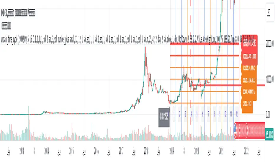
Wosabi Time Cycle Gann v1 This indicator is an auxiliary tool for drawing the five-year and ten-year cycle, as it draws vertical lines every 12 candles and for 12 minor cycles, so that a major cycle consists of 144 candles, which is the ten-year cycle. It helps to know whether the current trend will continue for the five-year cycle and whether it will complete the ten-year cycle or not The standard cycle assumes that the trend is from a bottom or a top, if it continues for more than 24 candles to 36 candles, then corrects and does not break the bottom or top, then the trend will continue at least to complete the five-year cycle, i.e. 72 candles, and if the trend continues and the seven-year cycle closes at the 82 candle above The price of the candle of the strategic line No. 42, there is a possibility to complete the ten-year cycle (you must have experience in the standard patterns of time cycles as explained by gan). The indicator also draws the digital gates in horizontal lines, and you have to select them manually and adjust the price difference from one currency to another from the settings. When adding the indicator for the first time, you must specify the candle of the beginning of the trend, whether at a bottom or a top, as well as specifying the highest or lowest price that is expected to reach five digital gates, and you can modify the gates later in the settings. You can show a horizontal line at the close of each minor cycle of 24 candles, and you can adjust the line length from the settings. You can also show lines on the vibration plugs. When the trend is up, the end price must be higher than the starting price, in order to draw the direction for the gates correctly, and when the trend is down, the end price must be lower than the starting price. Important note: This indicator depends on your experience in time cycles and will not give you any buy or sell signals. It is an indicator that saves you drawing for cycles and gates and depends on your personal experience in time cycles. هذا المؤشر اداة مساعدة لرسم دورة الخمس سنوات والعشر سنوات، فهو يرسم خطوط اعمده راسية كل 12 شمعة ولعدد 12 دورة صغرى لتتكون دورة كبرى من 144 شمعة وهي دورة العشر سنوات وهي تساعد لمعرفة هل الاتجاه الحالي سيستمر لدورة الخمس سنوات وهل سيكمل دورة العشر سنوات ام لا ، فالدورة القياسية تفترض ان الاتجاه من قاع او قمة اذا استمر لاكثر من 24 شمعة الى 36 شمعة ثم صحح ولم يكسر القاع او القمة فإن الاتجاه سيستمر على الاقل لاكمال دورة الخمس سنوات اي 72 شمعة ، واذا استمر الاتجاه واغلق دورة السبع سنوات عند الشمعة 82 فوق سعر شمعة خط الاستراتيجي رقم 42 فهنالك احتمالية لاكمال دورة العشر سنوات (يجب ان يكون ليك خبرة في الانماط القياسية للدورات الزمنية كما شرحها gan). كذلك يقوم المؤشر برسم البوابات الرقمية في خطوط افقية وعليك تحديدها بشكل يدوي وتعديل فارق السعر من عملة لاخرى من الاعدادات . عند اضافة المؤشر لاول مرة يجب تحديد شمعة بداية الاتجاه سواء عند قاع او قمة وكذلك تحديد السعر الاعلى او الادنى المتوقع ان تصل له خمس بوابات رقمية ويمكنك تعديل البوابات لاحقا من الاعدادات . يمكنك اظهار خط افقي عند اغلاق كل دورة صغرى لعدد 24 شمعة ويمكنك تعديل طول الخط من الاعدادات . يمكنك كذلك اظهار خطوط على شمعات الاهتزاز . عندما يكون الاتجاه صاعد يجب ان يكون سعر النهاية اعلى من سعر البداية ليتم رسم الاتتجاه للبوابات بشكل صحيح وعندما يكون الاتجاه هابط يجب ان يكون سعر النهاية ادنى من سعر البداية . ملاحظة هامة : هذا المؤشر يعتمد على خبرتك في الدورات الزمنية ولن يعطيك اي اشارات شراء او بيع فهو مؤشر يوفر عليك الرسم للدورات والبوابات ويعتمد على خبرتك الشخصية في الدورات الزمنية . Indicatore Pine Script®di AhmadWosabiAggiornato 66158
Fibonacci Cycle Finder🟩 Fibonacci Cycle Finder is an indicator designed to explore Fibonacci-based waves and cycles through visualization and experimentation, introducing a trigonometric approach to market structure analysis. Unlike traditional Fibonacci tools that rely on static horizontal levels, this indicator incorporates the dynamic nature of market cycles, using adjustable wavelength, phase, and amplitude settings to visualize the rhythm of price movements. By applying a sine function, it provides a structured way to examine Fibonacci relationships in a non-linear context. Fibonacci Cycle Finder unifies Fibonacci principles with a wave-based method by employing adjustable parameters to align each wave with real-time price action. By default, the wave begins with minimal curvature, preserving the structural familiarity of horizontal Fibonacci retracements. By adjusting the input parameters, the wave can subtly transition from a horizontal line to a more pronounced cycle,visualizing cyclical structures within price movement. This projective structure extends potential cyclical outlines on the chart, opening deeper exploration of how Fibonacci relationships may emerge over time. Fibonacci Cycle Finder further underscores a non-linear representation of price by illustrating how wave-based logic can uncover shifts that are missed by static retracement tools. Rather than imposing immediate oscillatory behavior, the indicator encourages a progressive approach, where the parameters may be incrementally modified to align wave structures with observed price action. This refinement process deepens the exploration of Fibonacci relationships, offering a systematic way to experiment with non-linear price dynamics. In doing so, it revisits fundamental Fibonacci concepts, demonstrating their broader adaptability beyond fixed horizontal retracements. 🌀 THEORY & CONCEPT 🌀 What if Fibonacci relationships could be visualized as dynamic waves rather than confined to fixed horizontal levels? Fibonacci Cycle Finder introduces a trigonometric approach to market structure analysis, offering a different perspective on Fibonacci-based cycles. This tool provides a way to visualize market fluctuations through cyclical wave motion, opening the door to further exploration of Fibonacci’s role in non-linear price behavior. Traditional Fibonacci tools, such as retracements and extensions, have long been used to identify potential support and resistance levels. While valuable for analyzing price trends, these tools assume linear price movement and rely on static horizontal levels. However, market fluctuations often exhibit cyclical tendencies , where price follows natural wave-like structures rather than strictly adhering to fixed retracement points. Although Fibonacci-based tools such as arcs, fans, and time zones attempt to address these patterns, they primarily apply geometric projections. The Fibonacci Cycle Finder takes a different approach by mapping Fibonacci ratios along structured wave cycles, aligning these relationships with the natural curvature of market movement rather than forcing them onto rigid price levels. Rather than replacing traditional Fibonacci methods, the Fibonacci Cycle Finder supplements existing Fibonacci theory by introducing an exploratory approach to price structure analysis. It encourages traders to experiment with how Fibonacci ratios interact with cyclical price structures, offering an additional layer of insight beyond static retracements and extensions. This approach allows Fibonacci levels to be examined beyond their traditional static form, providing deeper insights into market fluctuations. 📊 FIBONACCI WAVE IMPLEMENTATION 📊 The Fibonacci Cycle Finder uses two user-defined swing points, A and B, as the foundation for projecting these Fibonacci waves. It first establishes standard horizontal levels that correspond to traditional Fibonacci retracements, ensuring a baseline reference before wave adjustments are applied. By default, the wave is intentionally subtle— Wavelength is set to 1 , Amplitude is set to 1 , and Phase is set to 0 . In other words, the wave starts as “stretched out.” This allows a slow, measured start, encouraging users to refine parameters incrementally rather than producing abrupt oscillations. As these parameters are increased, the wave takes on more distinct sine and cosine characteristics, offering a flexible approach to exploring Fibonacci-based cyclicity within price action. Three parameters control the shape of the Fibonacci wave: 1️⃣ Wavelength Controls the horizontal spacing of the wave along the time axis, determining the length of one full cycle from peak to peak (or trough to trough). In this indicator, Wavelength acts as a scaling input that adjusts how far the wave extends across time, rather than a strict mathematical “wavelength.” Lower values further stretch the wave, increasing the spacing between oscillations, while higher values compress it into a more frequent cycle. Each full cycle is divided into four quarter-cycle segments, a deliberate design choice to minimize curvature by default. This allows for subtle oscillations and smoother transitions, preventing excessive distortion while maintaining flexibility in wave projections. The wavelength is calculated relative to the A-B swing, ensuring that its scale adapts dynamically to the selected price range. 2️⃣ Amplitude Defines the vertical displacement of the wave relative to the baseline Fibonacci level. Higher values increase the height of oscillations, while lower values reduce the height, Negative values will invert the wave’s initial direction. The amplitude is dynamically applied in relation to the A-B swing direction, ensuring that an upward swing results in upward oscillations and a downward swing results in downward oscillations. 3️⃣ Phase Shifts the wave’s starting position along its cycle, adjusting alignment relative to the swing points. A phase of 0 aligns with a sine wave, where the cycle starts at zero and rises. A phase of 25 aligns with a cosine wave, starting at a peak and descending. A phase of 50 inverts the sine wave, beginning at zero but falling first, while a phase of 75 aligns with an inverted cosine , starting at a trough and rising. Intermediate values between these phases create gradual shifts in wave positioning, allowing for finer alignment with observed market structures. By fine-tuning these parameters, users can adapt Fibonacci waves to better reflect observed market behaviors. The wave structure integrates with price movements rather than simply overlaying static levels, allowing for a more dynamic representation of cyclical price tendencies. This indicator serves as an exploratory tool for understanding potential market rhythms, encouraging traders to test and visualize how Fibonacci principles extend beyond their traditional applications. 🖼️ CHART EXAMPLES 🖼️ Following this downtrend, price interacts with curved Fibonacci levels, highlighting resistance at the 0.236 and 0.382 levels, where price stalls before pulling back. Support emerges at the 0.5, 0.618, and 0.786 levels, where price finds stability and rebounds In this Fibonacci retracement, price initially finds support at the 1.0 level, following the natural curvature of the cycle. Resistance forms at 0.786, leading to a pullback before price breaks through and tests 0.618 as resistance. Once 0.618 is breached, price moves upward to test 0.5, illustrating how Fibonacci-based cycles may align with evolving market structure beyond static, horizontal retracements. Following this uptrend, price retraces downward and interacts with the Fibonacci levels, demonstrating both support and resistance at key levels such as 0.236, 0.382, 0.5, and 0.618. With only the 0.5 and 1.0 levels enabled, this chart remains uncluttered while still highlighting key price interactions. The short cycle length results in a mild curvature, aligning smoothly with market movement. Price finds resistance at the 0.5 level while showing strong support at 1.0, which follows the natural flow of the market. Keeping the focus on fewer levels helps maintain clarity while still capturing how price reacts within the cycle. 🛠️ CONFIGURATION AND SETTINGS 🛠️ Wave Parameters Wavelength : Stretches or compresses the wave along the time axis, determining the length of one full cycle. Higher values extend the wave across more bars, while lower values compress it into a shorter time frame. Amplitude : Expands or contracts the wave along the price axis, determining the height of oscillations relative to Fibonacci levels. Higher values increase the vertical range, while negative values invert the wave’s initial direction. Phase : Offsets the wave along the time axis, adjusting where the cycle begins. Higher values shift the starting position forward within the wave pattern. Fibonacci Levels Levels : Enable or disable specific Fibonacci levels (0.0, 0.236, 0.382, 0.5, 0.618, 0.786, 1.0) to focus on relevant price zones. Color : Modify level colors for enhanced visual clarity. Visibility Trend Line/Color : Toggle and customize the trend line connecting swing points A and B. Setup Lines : Show or hide lines linking Fibonacci levels to projected waves. A/B Labels Visibility : Control the visibility of swing point labels. Left/Right Labels : Manage the display of Fibonacci level labels on both sides of the chart. Fill % : Adjust shading intensity between Fibonacci levels (0% = no fill, 100% = maximum fill). A and B Points (Time/Price): These user-defined anchor points serve as the basis for Fibonacci wave calculations and can be manually set. A and B points can also be adjusted directly on the chart, with automatic synchronization to the settings panel, allowing for seamless modifications without needing to manually input values. ⚠️ DISCLAIMER ⚠️ The Fibonacci Cycle Finder is a visual analysis tool designed to illustrate Fibonacci relationships and serve as a supplement to traditional Fibonacci tools. While the indicator employs mathematical and geometric principles, no guarantee is made that its calculations will align with other Fibonacci tools or proprietary methods. Like all technical and visual indicators, the Fibonacci levels generated by this tool may appear to visually align with key price zones in hindsight. However, these levels are not intended as standalone signals for trading decisions. This indicator is intended for educational and analytical purposes, complementing other tools and methods of market analysis. 🧠 BEYOND THE CODE 🧠 Fibonacci Cycle Finder is the latest indicator in the Fibonacci Geometry Series. Building on the concepts of the Fibonacci Time-Price Zones and the Fibonacci 3-D indicators, this tool introduces a trigonometric approach to market structure analysis. The Fibonacci Cycle Finder indicator, like other xxattaxx indicators , is designed to encourage both education and community engagement. Your feedback and insights are invaluable to refining and enhancing the Fibonacci Cycle Finder indicator. We look forward to the creative applications, observations, and discussions this tool inspires within the trading community.Indicatore Pine Script®di xxattaxxAggiornato 88584
Wosabi 2 Time Cycle Gann and candles v3Important Note: This indicator relies on your expertise in time cycles and does not provide any buy or sell signals. It helps you by automating the drawing of minor and major time cycles and digital gates, relying on your personal expertise. It simply draws a vertical line every 12 candles from your selected starting candle and repeats this until the cycle is complete after 12 minor cycles. Additionally, it calculates digital gates, and you need to configure the settings to choose the type of calculation for the digital gate, whether it's based on the commonly known digital gates (12-15-18) or gate targets, for example (369-693-936-258-582-825-147...), and then multiply them based on the price difference you input to draw horizontal lines for the expected gates. If a gate is broken, the price will continue to the next gate. This indicator is an auxiliary tool for drawing the five, seven, ten, and even fifty or more cycles that Gann discussed. With its default settings, it draws vertical lines every 12 candles for 12 minor cycles (modifiable), forming a major cycle of 144 candles, which is the ten-cycle. (You should have experience in time cycle patterns as explained by Gann to know if the trend will continue up or down over time). The indicator only draws the columns that define the minor cycles, and their total forms the major cycle. - The indicator also draws digital gates as horizontal lines, which you need to set manually and adjust the price difference from one currency to another in the settings. - When adding the indicator for the first time, you must specify the starting candle of the trend, whether at a bottom or a top, and determine the highest or lowest price expected to reach five digital gates. If you expect an upward cycle, set the price at the resistance area where you expect the price to bounce. If you want to draw a downward cycle, set the price at the support area where you expect the bounce. You can later adjust the gates from the settings if you want to calculate them according to the digital gate. For example, if you start drawing the downward cycle for Bitcoin, as in the above picture when the highest price was 73881, we add the first two digits 7+3=10, 1+0=1, and the number 1 corresponds to gate 12, so you select it from the settings and then adjust the price difference to 1000 or its multiples since Bitcoin's price is in thousands. If it is another currency with a price not exceeding $100, adjust the price difference to 10 or its multiples. Thus, adjust the price difference from one currency to another. For currencies with values in fractions, the price difference will be 0.0001 or the closest figure to the currency's price, as an example. - You can display a horizontal line at the close of each minor cycle, i.e., every 12 candles. - You can display a strategic line at candle 42 from the start of the cycle. The strategic line is used to guide you; if the trend is up and doesn't close below this line after 7 minor cycles, the trend will likely continue up, or above it if the trend is down. In a downtrend, there are slightly different rules that can't be fully explained here. - You can also display lines on the vibration candles, which are multiples of the number 3 from the start of the cycle, i.e., 3, 9, 12, 15, etc. - When the trend is upward, the ending price should be higher than the starting price to draw the trend towards the gates correctly. When the trend is downward, the ending price should be lower than the starting price. - You can now calculate digital gates in more than one way, and you can adjust the digital gates (if you have a specific method for calculating them), double them, or divide them. ** One of the most important additions is the ability to convert minor time cycles into candles to visualize the upcoming direction of the minor cycle. ملاحظة هامة : هذا المؤشر يعتمد على خبرتك في الدورات الزمنية ولن يعطيك اي اشارات شراء او بيع فهو مؤشر يوفر عليك الرسم للدورات الزمنية الصغرى والكبرى والبوابات الرقمية ويعتمد على خبرتك الشخصية وعمله ببساطه يقوم برسم خط عمودي كل 12 شمعة من بعد اختيارك لاي شمعة ويكرر رسم الاعمده حتى اكتمال الدورة بعد 12 دورة زمنية صغرى كما انه يقوم بحساب البوابات الرقمية ويجب عليك ضبط الاعدادات من المؤشر باختيار نوع الحساب للبوابة الرقمية هل هو حساب البوابات الرقمية المتعارف عليها ( 12-15-18) او حسب اهداف البوابات كمثال (369-693-936-258-582-825-147.....) ثن يتم مضاعفتها حسب ادخالك لفارق الاسعار ليتم رسم خطوط افقيه للبوابات المتوقع اذا كسرها يستمر السعر بالوصول للبوابة التي تليها . هذا المؤشر اداة مساعدة لرسم دورة الخمس او السبع اوالعشر وحتى الخمسين واكثر التي تحدث عنها gan ، فهو باعداداته الافتراضية يرسم خطوط اعمده راسية كل 12 شمعة ولعدد 12 دورة صغرى (يمكن تعديلها) لتتكون دورة كبرى من 144 شمعة وهي دورة العشرة ، (يجب ان يكون ليك خبرة في انماط الدورات الزمنية كما شرحها gan لتعرف هل سيستمر الصعود او الهبوط زمنياً ) فالمؤشر فقط يرسم الاعمدة التي تحدد الدورات الصغرى ومجموعها يكون الدورة الكبرى . - يقوم المؤشر ايضا برسم البوابات الرقمية في خطوط افقية وعليك تحديدها بشكل يدوي وتعديل فارق السعر من عملة لاخرى من الاعدادات . - عند اضافة المؤشر لاول مرة يجب تحديد شمعة بداية الاتجاه سواء عند قاع او قمة وكذلك تحديد السعر الاعلى او الادنى المتوقع ان تصل له خمس بوابات رقمية فاذا كنت تتوقع ان الدورة صاعدة فحينها تحدد السعر عند منطقة المقاومة التي تتوقع ان يرتد منها السعر وان كنت تريد رسم دورة هابطة فحينها تحدد السعر عند منطقة الدعم المتوقع الارتداد منه ويمكنك تعديل البوابات لاحقا من الاعدادات اذا اردت حسابها حسب البوابة الرقمية على سبيل المثال اذا رسمت بداية الدورة الهابطة للبيتكوين كما في الصورة اعلاه حينما كان سعر اعلى قمة 73881 نقوم بجمع اول رقمين و هم 7+3=10 , 1+0=1 والرقم 1 يتبع البوابه 12 فتقوم باختيارها من الاعدادات ثم تقوم بتعديل فارق السعر الى 1000 او مضاعفاته كون سعر البيتكوين بالالاف وان كانت عمله اخرى نفترض ان سعرها ل يتجاوز 100 دولار نعدل فارق السعر الى 10 او مضاعفاته وهكذا نقوم بتعديل فارق السعر من عملة الى اخرى ففي العملات الصفرية سيكون فارق السعر 0.0001 او حسب الرقم القريب لسعر العملة هذا فقط كمثال . - يمكنك اظهار خط افقي عند اغلاق كل دورة صغرى اي كل 12 سمعة . - يمكنك اظهار خط الاستراتيجي عند شمعة 42 من بداية الدورة وخط الاستراتيجي يسترشد من خلاله اذا لم يتم الاغلاق اسفله اذا كان الاتجاه صاعد بعد 7 دورات صغرى ان الاتجاه سيستمر او اعلاه اذا كان الاتجاه هابط وفي الاتجاه الهابط هنالك قواعد مختلفة قليلاً لا يتسع المجال لشرحها. - يمكنك كذلك اظهار خطوط على شمعات الاهتزاز التي تكون من بداية الدورة مضاعفات الرقم 3 اي 3,9,12,15 وهكذ . - عندما يكون الاتجاه صاعد يجب ان يكون سعر النهاية اعلى من سعر البداية ليتم رسم الاتتجاه للبوابات بشكل صحيح وعندما يكون الاتجاه هابط يجب ان يكون سعر النهاية ادنى من سعر البداية . - يمكنك الان حساب البوابات الرقمية باكثر من طريقة ويمكنك تعديل البوابات الرقمية (اذا كان لديك طريقة معينة لحسابها) او مضاعفتها او تقسيمها . ** من اهم الاضافات هو امكانية تحويل الدورات الزمنية الصغرة الى شموع حتى تتخيل الاتجاه القادم لحركة الدورة الصغرى .Indicatore Pine Script®di AhmadWosabi11114
Poly Cycle [Loxx]This is an example of what can be done by combining Legendre polynomials and analytic signals. I get a way of determining a smooth period and relative adaptive strength indicator without adding time lag. This indicator displays the following: The Least Squares fit of a polynomial to a DC subtracted time series - a best fit to a cycle. The normalized analytic signal of the cycle (signal and quadrature). The Phase shift of the analytic signal per bar. The Period and HalfPeriod lengths, in bars of the current cycle. A relative strength indicator of the time series over the cycle length. That is, adaptive relative strength over the cycle length. The Relative Strength Indicator, is adaptive to the time series, and it can be smoothed by increasing the length of decreasing the number of degrees of freedom. Other adaptive indicators based upon the period and can be similarly constructed. There is some new math here, so I have broken the story up into 5 Parts: Part 1: Any time series can be decomposed into a orthogonal set of polynomials . This is just math and here are some good references: Legendre polynomials - Wikipedia, the free encyclopedia Peter Seffen, "On Digital Smoothing Filters: A Brief Review of Closed Form Solutions and Two New Filter Approaches", Circuits Systems Signal Process, Vol. 5, No 2, 1986 I gave some thought to what should be done with this and came to the conclusion that they can be used for basic smoothing of time series. For the analysis below, I decompose a time series into a low number of degrees of freedom and discard the zero mode to introduce smoothing. That is: time series => c_1 t + c_2 t^2 ... c_Max t^Max This is the cycle. By construction, the cycle does not have a zero mode and more physically, I am defining the "Trend" to be the zero mode. The data for the cycle and the fit of the cycle can be viewed by setting ShowDataAndFit = TRUE; There, you will see the fit of the last bar as well as the time series of the leading edge of the fits. If you don't know what I mean by the "leading edge", please see some of the postings in . The leading edges are in grayscale, and the fit of the last bar is in color. I have chosen Length = 17 and Degree = 4 as the default. I am simply making sure by eye that the fit is reasonably good and degree 4 is the lowest polynomial that can represent a sine-like wave, and 17 is the smallest length that lets me calculate the Phase Shift (Part 3 below) using the Hilbert Transform of width=7 (Part 2 below). Depending upon the fit you make, you will capture different cycles in the data. A fit that is too "smooth" will not see the smaller cycles, and a fit that is too "choppy" will not see the longer ones. The idea is to use the fit to try to suppress the smaller noise cycles while keeping larger signal cycles. Part 2: Every time series has an Analytic Signal, defined by applying the Hilbert Transform to it. You can think of the original time series as amplitude * cosine(theta) and the transformed series, called the quadrature, can be thought of as amplitude * sine(theta). By taking the ratio, you can get the angle theta, and this is exactly what was done by John Ehlers in . It lets you get a frequency out of the time series under consideration. Amazon.com: Rocket Science for Traders: Digital Signal Processing Applications (9780471405672): John F. Ehlers: Books It helps to have more references to understand this. There is a nice article on Wikipedia on it. Read the part about the discrete Hilbert Transform: en.wikipedia.org If you really want to understand how to go from continuous to discrete, look up this article written by Richard Lyons: www.dspguru.com In the indicator below, I am calculating the normalized analytic signal, which can be written as: s + i h where i is the imagery number, and s^2 + h^2 = 1; s= signal = cosine(theta) h = Hilbert transformed signal = quadrature = sine(theta) The angle is therefore given by theta = arctan(h/s); The analytic signal leading edge and the fit of the last bar of the cycle can be viewed by setting ShowAnalyticSignal = TRUE; The leading edges are in grayscale fit to the last bar is in color. Light (yellow) is the s term, and Dark (orange) is the quadrature (hilbert transform). Note that for every bar, s^2 + h^2 = 1 , by construction. I am using a width = 7 Hilbert transform, just like Ehlers. (But you can adjust it if you want.) This transform has a 7 bar lag. I have put the lag into the plot statements, so the cycle info should be quite good at displaying minima and maxima (extrema). Part 3: The Phase shift is the amount of phase change from bar to bar. It is a discrete unitary transformation that takes s + i h to s + i h explicitly, T = (s+ih)*(s -ih ) , since s *s + h *h = 1. writing it out, we find that T = T1 + iT2 where T1 = s*s + h*h and T2 = s*h -h*s and the phase shift is given by PhaseShift = arctan(T2/T1); Alas, I have no reference for this, all I doing is finding the rotation what takes the analytic signal at bar to the analytic signal at bar . T is the transfer matrix. Of interest is the PhaseShift from the closest two bars to the present, given by the bar and bar since I am using a width=7 Hilbert transform, bar is the earliest bar with an analytic signal. I store the phase shift from bar to bar as a time series called PhaseShift. It basically gives you the (7-bar delayed) leading edge the amount of phase angle change in the series. You can see it by setting ShowPhaseShift=TRUE The green points are positive phase shifts and red points are negative phase shifts. On most charts, I have looked at, the indicator is mostly green, but occasionally, the stock "retrogrades" and red appears. This happens when the cycle is "broken" and the cycle length starts to expand as a trend occurs. Part 4: The Period: The Period is the number of bars required to generate a sum of PhaseShifts equal to 360 degrees. The Half-period is the number of bars required to generate a sum of phase shifts equal to 180 degrees. It is usually not equal to 1/2 of the period. You can see the Period and Half-period by setting ShowPeriod=TRUE The code is very simple here: Value1=0; Value2=0; while Value1 < bar_index and math.abs(Value2) < 360 begin Value2 = Value2 + PhaseShift ; Value1 = Value1 + 1; end; Period = Value1; The period is sensitive to the input length and degree values but not overly so. Any insight on this would be appreciated. Part 5: The Relative Strength indicator: The Relative Strength is just the current value of the series minus the minimum over the last cycle divided by the maximum - minimum over the last cycle, normalized between +1 and -1. RelativeStrength = -1 + 2*(Series-Min)/(Max-Min); It therefore tells you where the current bar is relative to the cycle. If you want to smooth the indicator, then extend the period and/or reduce the polynomial degree. In code: NewLength = floor(Period + HilbertWidth+1); Max = highest(Series,NewLength); Min = lowest(Series,NewLength); if Max>Min then Note that the variable NewLength includes the lag that comes from the Hilbert transform, (HilbertWidth=7 by default). Conclusion: This is an example of what can be done by combining Legendre polynomials and analytic signals to determine a smooth period without adding time lag. ________________________________ Changes in this one : instead of using true/false options for every single way to display, use Type parameter as following : 1. The Least Squares fit of a polynomial to a DC subtracted time series - a best fit to a cycle. 2. The normalized analytic signal of the cycle (signal and quadrature). 3. The Phase shift of the analytic signal per bar. 4. The Period and HalfPeriod lengths, in bars of the current cycle. 5. A relative strength indicator of the time series over the cycle length. That is, adaptive relative strength over the cycle length.Indicatore Pine Script®di loxxAggiornato 44155
Adaptivity: Measures of Dominant Cycles and Price Trend [Loxx]Adaptivity: Measures of Dominant Cycles and Price Trend is an indicator that outputs adaptive lengths using various methods for dominant cycle and price trend timeframe adaptivity. While the information output from this indicator might be useful for the average trader in one off circumstances, this indicator is really meant for those need a quick comparison of dynamic length outputs who wish to fine turn algorithms and/or create adaptive indicators. This indicator compares adaptive output lengths of all publicly known adaptive measures. Additional adaptive measures will be added as they are discovered and made public. The first released of this indicator includes 6 measures. An additional three measures will be added with updates. Please check back regularly for new measures. Ehers: Autocorrelation Periodogram Band-pass Instantaneous Cycle Hilbert Transformer Dual Differentiator Phase Accumulation (future release) Homodyne (future release) Jurik: Composite Fractal Behavior (CFB) Adam White: Veritical Horizontal Filter (VHF) (future release) What is an adaptive cycle, and what is Ehlers Autocorrelation Periodogram Algorithm? From his Ehlers' book Cycle Analytics for Traders Advanced Technical Trading Concepts by John F. Ehlers , 2013, page 135: "Adaptive filters can have several different meanings. For example, Perry Kaufman's adaptive moving average (KAMA) and Tushar Chande's variable index dynamic average (VIDYA) adapt to changes in volatility . By definition, these filters are reactive to price changes, and therefore they close the barn door after the horse is gone.The adaptive filters discussed in this chapter are the familiar Stochastic , relative strength index (RSI), commodity channel index (CCI), and band-pass filter.The key parameter in each case is the look-back period used to calculate the indicator. This look-back period is commonly a fixed value. However, since the measured cycle period is changing, it makes sense to adapt these indicators to the measured cycle period. When tradable market cycles are observed, they tend to persist for a short while.Therefore, by tuning the indicators to the measure cycle period they are optimized for current conditions and can even have predictive characteristics. The dominant cycle period is measured using the Autocorrelation Periodogram Algorithm. That dominant cycle dynamically sets the look-back period for the indicators. I employ my own streamlined computation for the indicators that provide smoother and easier to interpret outputs than traditional methods. Further, the indicator codes have been modified to remove the effects of spectral dilation.This basically creates a whole new set of indicators for your trading arsenal." What is this Hilbert Transformer? An analytic signal allows for time-variable parameters and is a generalization of the phasor concept, which is restricted to time-invariant amplitude, phase, and frequency. The analytic representation of a real-valued function or signal facilitates many mathematical manipulations of the signal. For example, computing the phase of a signal or the power in the wave is much simpler using analytic signals. The Hilbert transformer is the technique to create an analytic signal from a real one. The conventional Hilbert transformer is theoretically an infinite-length FIR filter. Even when the filter length is truncated to a useful but finite length, the induced lag is far too large to make the transformer useful for trading. From his Ehlers' book Cycle Analytics for Traders Advanced Technical Trading Concepts by John F. Ehlers , 2013, pages 186-187: "I want to emphasize that the only reason for including this section is for completeness. Unless you are interested in research, I suggest you skip this section entirely. To further emphasize my point, do not use the code for trading. A vastly superior approach to compute the dominant cycle in the price data is the autocorrelation periodogram. The code is included because the reader may be able to capitalize on the algorithms in a way that I do not see. All the algorithms encapsulated in the code operate reasonably well on theoretical waveforms that have no noise component. My conjecture at this time is that the sample-to-sample noise simply swamps the computation of the rate change of phase, and therefore the resulting calculations to find the dominant cycle are basically worthless.The imaginary component of the Hilbert transformer cannot be smoothed as was done in the Hilbert transformer indicator because the smoothing destroys the orthogonality of the imaginary component." What is the Dual Differentiator, a subset of Hilbert Transformer? From his Ehlers' book Cycle Analytics for Traders Advanced Technical Trading Concepts by John F. Ehlers , 2013, page 187: "The first algorithm to compute the dominant cycle is called the dual differentiator. In this case, the phase angle is computed from the analytic signal as the arctangent of the ratio of the imaginary component to the real component. Further, the angular frequency is defined as the rate change of phase. We can use these facts to derive the cycle period." What is the Phase Accumulation, a subset of Hilbert Transformer? From his Ehlers' book Cycle Analytics for Traders Advanced Technical Trading Concepts by John F. Ehlers , 2013, page 189: "The next algorithm to compute the dominant cycle is the phase accumulation method. The phase accumulation method of computing the dominant cycle is perhaps the easiest to comprehend. In this technique, we measure the phase at each sample by taking the arctangent of the ratio of the quadrature component to the in-phase component. A delta phase is generated by taking the difference of the phase between successive samples. At each sample we can then look backwards, adding up the delta phases.When the sum of the delta phases reaches 360 degrees, we must have passed through one full cycle, on average.The process is repeated for each new sample. The phase accumulation method of cycle measurement always uses one full cycle's worth of historical data.This is both an advantage and a disadvantage.The advantage is the lag in obtaining the answer scales directly with the cycle period.That is, the measurement of a short cycle period has less lag than the measurement of a longer cycle period. However, the number of samples used in making the measurement means the averaging period is variable with cycle period. longer averaging reduces the noise level compared to the signal.Therefore, shorter cycle periods necessarily have a higher out- put signal-to-noise ratio." What is the Homodyne, a subset of Hilbert Transformer? From his Ehlers' book Cycle Analytics for Traders Advanced Technical Trading Concepts by John F. Ehlers , 2013, page 192: "The third algorithm for computing the dominant cycle is the homodyne approach. Homodyne means the signal is multiplied by itself. More precisely, we want to multiply the signal of the current bar with the complex value of the signal one bar ago. The complex conjugate is, by definition, a complex number whose sign of the imaginary component has been reversed." What is the Instantaneous Cycle? The Instantaneous Cycle Period Measurement was authored by John Ehlers; it is built upon his Hilbert Transform Indicator. From his Ehlers' book Cybernetic Analysis for Stocks and Futures: Cutting-Edge DSP Technology to Improve Your Trading by John F. Ehlers, 2004, page 107: "It is obvious that cycles exist in the market. They can be found on any chart by the most casual observer. What is not so clear is how to identify those cycles in real time and how to take advantage of their existence. When Welles Wilder first introduced the relative strength index (rsi), I was curious as to why he selected 14 bars as the basis of his calculations. I reasoned that if i knew the correct market conditions, then i could make indicators such as the rsi adaptive to those conditions. Cycles were the answer. I knew cycles could be measured. Once i had the cyclic measurement, a host of automatically adaptive indicators could follow. Measurement of market cycles is not easy. The signal-to-noise ratio is often very low, making measurement difficult even using a good measurement technique. Additionally, the measurements theoretically involve simultaneously solving a triple infinity of parameter values. The parameters required for the general solutions were frequency, amplitude, and phase. Some standard engineering tools, like fast fourier transforms (ffs), are simply not appropriate for measuring market cycles because ffts cannot simultaneously meet the stationarity constraints and produce results with reasonable resolution. Therefore i introduced maximum entropy spectral analysis (mesa) for the measurement of market cycles. This approach, originally developed to interpret seismographic information for oil exploration, produces high-resolution outputs with an exceptionally short amount of information. A short data length improves the probability of having nearly stationary data. Stationary data means that frequency and amplitude are constant over the length of the data. I noticed over the years that the cycles were ephemeral. Their periods would be continuously increasing and decreasing. Their amplitudes also were changing, giving variable signal-to-noise ratio conditions. Although all this is going on with the cyclic components, the enduring characteristic is that generally only one tradable cycle at a time is present for the data set being used. I prefer the term dominant cycle to denote that one component. The assumption that there is only one cycle in the data collapses the difficulty of the measurement process dramatically." What is the Band-pass Cycle? From his Ehlers' book Cycle Analytics for Traders Advanced Technical Trading Concepts by John F. Ehlers , 2013, page 47: "Perhaps the least appreciated and most underutilized filter in technical analysis is the band-pass filter. The band-pass filter simultaneously diminishes the amplitude at low frequencies, qualifying it as a detrender, and diminishes the amplitude at high frequencies, qualifying it as a data smoother. It passes only those frequency components from input to output in which the trader is interested. The filtering produced by a band-pass filter is superior because the rejection in the stop bands is related to its bandwidth. The degree of rejection of undesired frequency components is called selectivity. The band-stop filter is the dual of the band-pass filter. It rejects a band of frequency components as a notch at the output and passes all other frequency components virtually unattenuated. Since the bandwidth of the deep rejection in the notch is relatively narrow and since the spectrum of market cycles is relatively broad due to systemic noise, the band-stop filter has little application in trading." From his Ehlers' book Cycle Analytics for Traders Advanced Technical Trading Concepts by John F. Ehlers , 2013, page 59: "The band-pass filter can be used as a relatively simple measurement of the dominant cycle. A cycle is complete when the waveform crosses zero two times from the last zero crossing. Therefore, each successive zero crossing of the indicator marks a half cycle period. We can establish the dominant cycle period as twice the spacing between successive zero crossings." What is Composite Fractal Behavior (CFB)? All around you mechanisms adjust themselves to their environment. From simple thermostats that react to air temperature to computer chips in modern cars that respond to changes in engine temperature, r.p.m.'s, torque, and throttle position. It was only a matter of time before fast desktop computers applied the mathematics of self-adjustment to systems that trade the financial markets. Unlike basic systems with fixed formulas, an adaptive system adjusts its own equations. For example, start with a basic channel breakout system that uses the highest closing price of the last N bars as a threshold for detecting breakouts on the up side. An adaptive and improved version of this system would adjust N according to market conditions, such as momentum, price volatility or acceleration. Since many systems are based directly or indirectly on cycles, another useful measure of market condition is the periodic length of a price chart's dominant cycle, (DC), that cycle with the greatest influence on price action. The utility of this new DC measure was noted by author Murray Ruggiero in the January '96 issue of Futures Magazine. In it. Mr. Ruggiero used it to adaptive adjust the value of N in a channel breakout system. He then simulated trading 15 years of D-Mark futures in order to compare its performance to a similar system that had a fixed optimal value of N. The adaptive version produced 20% more profit! This DC index utilized the popular MESA algorithm (a formulation by John Ehlers adapted from Burg's maximum entropy algorithm, MEM). Unfortunately, the DC approach is problematic when the market has no real dominant cycle momentum, because the mathematics will produce a value whether or not one actually exists! Therefore, we developed a proprietary indicator that does not presuppose the presence of market cycles. It's called CFB (Composite Fractal Behavior) and it works well whether or not the market is cyclic. CFB examines price action for a particular fractal pattern, categorizes them by size, and then outputs a composite fractal size index. This index is smooth, timely and accurate Essentially, CFB reveals the length of the market's trending action time frame. Long trending activity produces a large CFB index and short choppy action produces a small index value. Investors have found many applications for CFB which involve scaling other existing technical indicators adaptively, on a bar-to-bar basis. What is VHF Adaptive Cycle? Vertical Horizontal Filter (VHF) was created by Adam White to identify trending and ranging markets. VHF measures the level of trend activity, similar to ADX DI. Vertical Horizontal Filter does not, itself, generate trading signals, but determines whether signals are taken from trend or momentum indicators. Using this trend information, one is then able to derive an average cycle length. Indicatore Pine Script®di loxxAggiornato 88141
Institutional Cycle Intelligence System (Machine Learning) The Institutional Cycle Intelligence System (Machine Learning) represents a paradigmatic shift in the capabilities of retail trading analysis, bridging the substantial divide between standard technical analysis and the rigorous, mathematically intensive domain of quantitative finance. At its core, this system is not merely an indicator but a sophisticated ensemble engine that synthesizes advanced Digital Signal Processing (DSP), spectral analysis, and modern Machine Learning techniques into a singular, cohesive market view. For quantitative analysts and institutional traders, this script serves as a testament to the power of "higher mathematics" applied to the chaotic, non-stationary nature of financial time series data. It moves beyond the lagging nature of time-domain indicators—like moving averages or the RSI—and operates primarily in the frequency domain, attempting to deconstruct price action into its constituent oscillatory components. This approach acknowledges a fundamental truth of market mechanics: that price is a composite signal, a noisy waveform comprised of underlying trends, cyclical harmonics, and stochastic noise. By isolating these components, the system offers a look into the "heartbeat" of market liquidity and institutional accumulation-distribution cycles. The defining characteristic that elevates this system to an institutional grade is its refusal to rely on a single mathematical model. Financial markets are dynamic systems; they shift between trending, mean-reverting, and chaotic regimes. A model that excels in a clean sine-wave market, like a standard cycle, will fail primarily during strong trends or high-volatility shocks. To solve this, the system employs an "Ensemble Architecture," running seven distinct, high-level mathematical models simultaneously. It creates a "committee of experts," where each algorithm analyzes the market through a different mathematical lens—some statistical, some spectral, and some decompositional. However, the true innovation lies in the integration of a Gradient Boosting Machine (GBM). This is where the concept becomes a game-changer for Pine Script development. The system does not merely average these models; it employs a machine learning layer that dynamically optimizes the weight of each model based on its recent predictive performance. It "learns" which mathematical approach is currently syncing best with the market's behavior and amplifies that signal while dampening the others. This is an application of adaptive filtering and optimization theory that is rarely seen outside of proprietary high-frequency trading desks. To understand the gravity of the mathematics involved, one must examine the specific algorithms employed, starting with the Ehlers Bandpass Filter and Hilbert Transform. This component is rooted in electrical engineering and signal processing. The Bandpass filter is designed to reject frequencies outside a specific range, effectively stripping away the high-frequency noise (tick-by-tick randomness) and low-frequency trends (macro-economic drift) to isolate the "tradable" cycle. Once isolated, the script applies the Hilbert Transform, a linear operator that produces the analytic representation of the signal. By converting the real-valued price series into the complex plane (creating real and imaginary components), the system can mathematically calculate the instantaneous phase and amplitude of the cycle. This allows for the precise determination of market turning points without the lag associated with traditional smoothing, effectively solving the "phase delay" problem that plagues standard oscillators. Complementing the classic DSP approach is the MESA (Maximum Entropy Spectral Analysis) model. Standard Fourier analysis assumes that data outside the observation window repeats or is zero, which creates "spectral leakage" and inaccuracies when analyzing short data bursts typical of trading. MESA, however, is based on information theory. It constructs a model that maximizes the entropy (randomness) of the unobserved data, thereby making the fewest assumptions possible about what the market did before or after the sample size. This results in a high-resolution estimation of cycle periods even with limited data points. It is a highly mathematical approach to autoregressive modeling, allowing the system to detect shifting cycle lengths rapidly as market volatility expands or contracts. The system also integrates the Goertzel Algorithm, a method optimized for detecting specific frequency components within a signal. While a Fast Fourier Transform (FFT) scans the entire frequency spectrum, the Goertzel algorithm acts as a matched filter, surgically interrogating the price data for the presence of specific, pre-defined cycle periods (Short, Medium, and Long). It computes the energy or "power" at these specific frequencies. For a quant, this is akin to tuning a radio receiver to listen specifically for the presence of institutional order flow frequencies. If the "power" at the 20-bar cycle is high, the Goertzel component signals that this specific harmonic is currently driving price action. This selective frequency analysis is computationally efficient and provides a direct measurement of cycle strength, distinguishing between a genuine cycle and random market drift. Moving into the realm of non-linear and non-stationary analysis, the system employs Empirical Mode Decomposition (EMD). Developed for analyzing data that is neither linear nor stationary—a perfect description of financial markets—EMD does not assume a fixed basis like sine waves. Instead, it uses a recursive "sifting" process to decompose the price into a finite number of Intrinsic Mode Functions (IMFs). The algorithm identifies local maxima and minima, creates upper and lower envelopes using cubic splines, and subtracts the mean of these envelopes from the data. This process is repeated until true oscillatory modes are extracted. EMD is often referred to as the "Hilbert-Huang Transform" in academic literature and is considered one of the most powerful tools for analyzing natural phenomena. By using EMD, the system can adapt to asymmetric cycles (where the rally is fast and the drop is slow) that linear models like the Fourier transform would misinterpret. The inclusion of Singular Spectrum Analysis (SSA) further deepens the mathematical rigor. SSA is a nonparametric spectral estimation method that combines elements of classical time series analysis, multivariate geometry, and signal processing. Conceptually, it involves embedding the time series into a vector space to form a "trajectory matrix" and then performing a decomposition (similar to Principal Component Analysis or SVD) to separate the series into independent components representing trend, oscillatory signals, and noise. While Pine Script limits the full matrix algebra required for complete SVD, the implementation here utilizes heuristic approximations to achieve the decompositional effect. This allows the system to filter out noise "subspaces," reconstructing a signal that retains the structural integrity of the market movement while discarding the stochastic "fuzz" that leads to false signals. Wavelet Analysis is utilized to address the "Heisenberg Uncertainty Principle" of signal processing, which states one cannot know the precise frequency and precise time of an event simultaneously. While Fourier analysis loses time resolution to gain frequency resolution, Wavelets use "short" basis functions for high frequencies and "long" basis functions for low frequencies. This Multi-Resolution Analysis (MRA) allows the system to see the forest and the trees simultaneously. It decomposes price energy across different scales, identifying whether volatility is driven by short-term microstructure noise or long-term structural shifts. The calculation of "Wavelet Energy" within the script provides a distinct metric of market state, often preceding explosive moves when energy clusters across multiple timescales. Finally, the statistical backbone is provided by Autocorrelation. This is the mathematical study of self-similarity. It calculates the correlation of the price series with a lagged version of itself. By scanning through various lags (periods), the algorithm identifies the time shift that produces the highest correlation coefficient. If price correlates highly with itself from 20 bars ago, it confirms a 20-bar cycle memory in the market. This is a purely statistical validation method that serves as a "sanity check" for the more complex spectral models, ensuring that the detected cycles are statistically significant and not artifacts of curve fitting. The culmination of these seven mathematical titans is the Gradient Boosting Machine (GBM) optimization layer. In the context of Pine Script, this is a revolutionary concept. Traditional indicators have static parameters; they calculate the same way in a crash as they do in a bull run. This system, however, utilizes a simplified machine learning loop. It calculates the "loss" or error of each of the seven models relative to recent price returns. Using a gradient descent-inspired approach, it updates a weight vector, assigning higher influence to models that have been predictive in the recent lookback window and penalizing those that have failed. If the market enters a choppy period where trends vanish, the EMD and Wavelet models (which handle noise well) might gain dominance, while the Trend-following components are suppressed. If the market enters a clean harmonic swing, the Ehlers and Goertzel models will take the lead. This dynamic adaptation makes the system "alive," capable of morphing its internal logic to match the current market regime. For the quantitative analyst, this system offers a robust framework for algorithmic strategy development. It provides "feature engineering" out of the box—transforming raw price data into normalized, de-trended, and phase-aligned oscillators. The composite signal is not just a line on a chart; it is a probability-weighted vector of market state. The "Zero-Lag" nature of the phase calculations allows for entry and exit precision that moving averages mathematically cannot provide. Furthermore, the decomposition of market movements into Short, Medium, and Long cycles allows for fractal analysis—identifying moments of "Constructive Interference" where all three cycles align in phase, creating high-probability, high-velocity trade setups often associated with institutional order execution. In conclusion, the Institutional Cycle Intelligence System (Machine Learning) is a tour de force of applied mathematics and computational finance. It transcends the limitations of standard technical analysis by treating the market not as a visual pattern, but as a complex signal processing problem. By leveraging the orthogonality of different mathematical approaches—spectral, statistical, and decompositional—and fusing them through an adaptive machine learning mechanism, it offers a level of insight typically reserved for hedge funds with dedicated quant teams. It demonstrates that Pine Script is no longer just a scripting language for drawing lines, but a viable environment for implementing complex, adaptive, and mathematically rigorous trading systems. It is a tool for those who understand that in the financial markets, the edge lies not in predicting the future, but in deeply understanding the mathematical structure of the present. Indicatore Pine Script®di jaydesaigu13
Vicious Cycle 1.2 [CR] - Enhanced█ OVERVIEW Vicious Cycle 1.2 is an advanced oscillator-based momentum indicator designed to identify high-probability reversal and continuation setups. This new version features adaptive threshold technology, visual trend state classification, and a higher timeframe alignment system to filter low-quality signals. The indicator analyzes multiple timeframe components and market dynamics to generate a composite momentum score, which is then smoothed and compared against statistical thresholds. Unlike traditional static oscillators, Vicious Cycle adapts its sensitivity zones to current market conditions, reducing false signals during volatile periods and increasing responsiveness during consolidation. █ FEATURES Adaptive Threshold System The indicator employs percentile-based threshold calculations that automatically adjust to recent market behavior. This ensures optimal signal generation across different instruments and market regimes without manual recalibration. • Toggle between dynamic and fixed threshold modes • Adjustable lookback period for threshold calculation (50-500 bars) • Customizable percentile levels for sensitivity tuning • Separate calibration for overbought and oversold zones Visual Trend State Classification Background coloring provides instant visual feedback on market condition strength without requiring analysis of indicator position. The six-state classification system combines oscillator position with signal line relationship to identify: • Strong bullish momentum • Moderate bullish bias • Weak bullish condition • Weak bearish condition • Moderate bearish bias • Strong bearish momentum Higher Timeframe Trend Alignment An optional filtering system analyzes higher timeframe trend direction to block counter-trend signals. Two modes are available: • Single EMA Mode: Uses price position relative to a customizable moving average • Dual EMA Mode: Employs fast and slow moving average crossover logic The filter only permits long signals during bullish trends and short signals during bearish trends, significantly improving signal quality in trending markets. Signal Detection Modes Multiple signal generation methods accommodate different trading styles: • Zone-Based Signals: Fires when oscillator crosses key threshold levels • Signal Line Cross: Generates entries based on oscillator and signal line interaction Comprehensive Alert System Pre-configured alert conditions cover all major indicator events: • Primary signal alerts (zone cross and signal line methods) • Zone entry and exit warnings • Extreme level notifications • Trend filter status changes • Convenience aggregators for "any long" or "any short" condition █ HOW TO USE Initial Configuration The indicator ships with optimized default settings suitable for most instruments and timeframes. New users should observe the indicator's behavior for at least 50 signals before adjusting parameters. 1 — Add the indicator to your chart and leave default settings unchanged. 2 — Monitor signal generation and background color transitions for several trading sessions. 3 — Set up basic alerts using the "ANY LONG Signal" and "ANY SHORT Signal" conditions. 4 — After observation period, adjust sensitivity based on your instrument's characteristics. Threshold Configuration For instruments with higher volatility, increase the percentile values (example: 90/75 instead of 85/65). For ranging or lower volatility instruments, decrease percentile values (example: 80/60 or 75/55). The lookback period controls how quickly thresholds adapt to changing conditions. Longer lookbacks (150-200) provide smoother adaptation, while shorter lookbacks (50-75) offer more responsive adjustments. Trend Filter Guidelines Enable the trend filter in clearly trending markets to reduce whipsaw trades. In ranging or choppy conditions, consider disabling the filter or using a shorter EMA period. • For position trading: Use 200-period single EMA • For swing trading: Use 150-period single EMA or 50/200 dual EMA • For day trading: Use 100-period single EMA or 50/100 dual EMA If the filter blocks all signals, the market may be ranging near the trend reference level. This is intentional behavior designed to keep you out of low-probability setups. Signal Interpretation Primary signals occur when the oscillator crosses threshold zones or intersects the signal line in extreme regions. The strongest setups combine: • Signal generation in the expected direction • Background color matching the trade direction (bright colors indicate high conviction) • Trend filter alignment • Price action confirmation at key support or resistance levels █ NOTES Alert Configuration Alerts must be manually configured in TradingView and do not activate automatically. Access the alert menu by clicking the indicator name and selecting "Add Alert on Vicious Cycle 1.2...". Choose your desired condition from the dropdown menu and configure notification preferences. We recommend starting with the aggregated "ANY" alerts rather than subscribing to all individual signal types, as this prevents notification overload during active market periods. Dynamic Threshold Behavior The adaptive threshold system requires sufficient historical data (minimum equal to the lookback period setting) to calculate percentiles accurately. During the initial bars, threshold values may appear unusual until adequate history accumulates. This is expected behavior and resolves automatically. Performance Considerations The indicator performs percentile calculations on each bar using array operations. While optimized for efficiency, users experiencing performance issues on lower-end devices may reduce the dynamic lookback period or disable the adaptive threshold feature to use fixed thresholds instead. Compatibility Vicious Cycle 1.2 is built on Pine Script version 6 and works on all instrument types and timeframes. The indicator does not repaint—all signals finalize at bar close. Historical signals remain stable and do not change with additional price data. █ RISK DISCLOSURE This indicator is an analytical tool and does not constitute financial advice. No indicator or trading system guarantees profitable results. Always employ proper risk management, position sizing, and stop-loss protocols. Past performance does not indicate future results. Users are responsible for their own trading decisions and outcomes.Indicatore Pine Script®Script a pagamentodi theheirophant66118
Pi Cycle BTC Top + Pre-Alert BandsPi Cycle BTC Top + Pre-Alert Bands is an advanced implementation of the classic Pi Cycle Top model, designed for Bitcoin cycle analysis on higher timeframes (especially 1D BTCUSD/BTCUSD·INDEX). The original Pi Cycle Top uses two moving averages: • 111-day SMA (short MA) • 350-day SMA ×2 (long MA) A Pi Top is signaled when the 111 SMA crosses above the 350×2 SMA. Historically, this has occurred near major BTC cycle highs. This script extends that idea with a 3-step early-warning sequence: • Pi Green – early compression: short/long MA ratio crosses upward into the green band (convergence from below is required). • Pi Yellow – mid-cycle warning: only fires if a valid Green has already occurred in the same cycle. • Pi Cycle Top – final top: the classic Pi Cycle cross, limited to one top signal per cycle. After a top, no new Yellow or Top signals can appear until a new Green event starts the next cycle. Background shading shows the active phase (Green / Yellow / late-cycle zone), so you can see at a glance where BTC is within its Pi-based macro structure. All logic is non-repainting: request.security() uses lookahead_off and no future data is accessed. Typical use This indicator is intended as a macro-cycle timing and risk-awareness tool, not a stand-alone entry system. Many traders use it to: • Watch for Pi Green as the start of a potential late-cycle advance. • Treat Pi Yellow as a rising-risk environment and tighten risk management. • Use the Pi Cycle Top as a historical high-risk zone where large profit-taking or hedging may be considered. Always combine this with your own analysis (trend, volume, on-chain, macro) before making decisions. How to set alerts Add the indicator to your chart (1D BTCUSD or BTCUSD·INDEX recommended). Click Alerts → Condition → Pi Cycle BTC Top + Pre-Alert Bands. Choose one of: • Pi Cycle – Green Pre-Alert (early convergence) • Pi Cycle – Yellow Pre-Alert (after Green only) • Pi Cycle – TOP (Single per Cycle, after Green) Use “Once per bar close” for higher-timeframe reliability. Disclaimer This tool is for educational and analytical purposes only. The Pi Cycle concept is based on historical behavior and does not guarantee future results. This is not financial advice; always do your own research and manage risk appropriately.Indicatore Pine Script®di KOMMODO_IO30
Fetch cycles This script tracks cycles in the market, specifically aiming to identify the cycle low and visually represent the cycle on the chart. It begins by initializing a cycle that spans 55 days (configurable) and incorporates a deviation margin for approximation. The script increments the day count from a defined start date (December 15, 2018) and looks for potential cycle lows after a specified number of days (50). Once a low is detected, using a comparison of the current price against the low from 4 days prior (configurable), the day count resets, and the script begins a new cycle. The cycle low is visually marked with a triangle below the bar where the low is confirmed. Dots are plotted on the chart to indicate the days leading up to the cycle low, with one set of dots appearing 5 days before the low and another set plotted closer to the cycle end. Additionally, the script tracks the days since the last cycle ended, and the start of the first cycle is marked with a blue triangle. This provides a clear visual indicator of the current cycle's progression and approximations of when the next low may occur.Indicatore Pine Script®di FetchTeamAggiornato 25