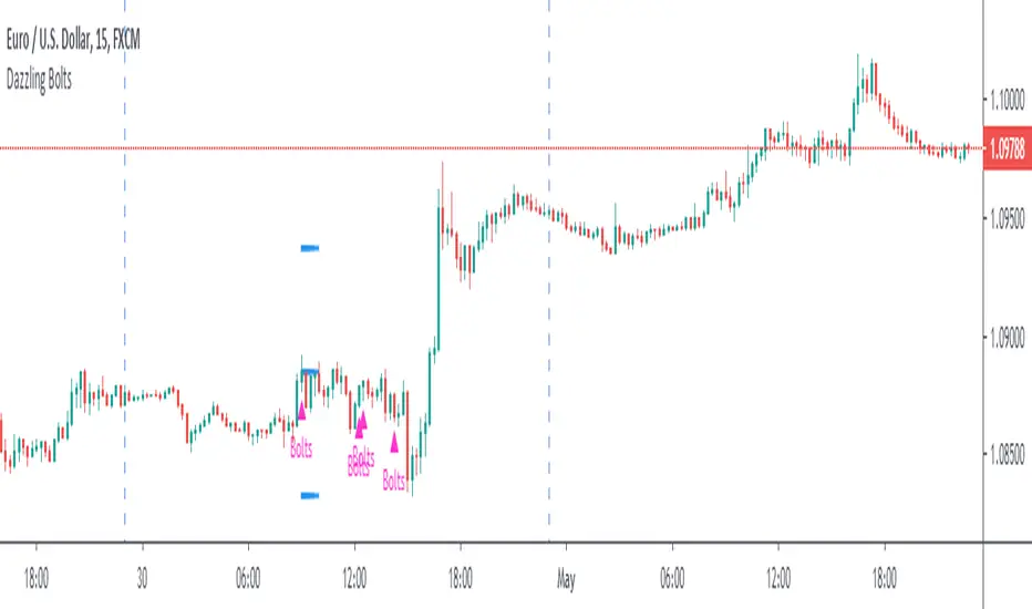
Dazzling BoltsThis is three moving average based strategy focused on trend-following. Targets and stops are set based on ATR. Following image pictures the strategy with all mas plotted:
Buying conditions are:
►A smoothened moving average (red) is above the exponential moving average (yellow)
►An exponential moving average is above simple moving average (black)
►Low five candles ago was still above the exponential moving average
►Low two candles ago reached below the exponential moving average
►Close of the previous candle was above the exponential moving average
►Ema force is disabled or exponential moving average set candles ago (orange) is still above simple moving average now.
If these conditions are met, Dazzling Bolts will always give you a signal. However, it holds only one position at a time and it will not buy again until it is closed or exited.
There are two ways exiting may happen. Smoothened moving average crosses below simple moving average or it reaches value based on your settings of average true range and its multiplier.
Settings 10/76/200/true/50/true/true/5/5 shows perfect results on EURUSD 15m chart but it does not guarantee the results. It is only 62 trades which is barely a useful statistical source. It is also highly optimized which means its settings filters out bad trades that may be bad only because of randomnation rather than set market behaviour. You need to test it on 200 trades + before using.
Cerca negli script per "Exponential"
VOLUME WEIGHTED MACD V2 VWMACDV2 BY KIVANÇ fr3762Second version of Buff Dormeier's Volume Weighted MACD indicator....
Here in this version; Exponential Moving Averages used and Weighted by Volume instead of using only vwma ( Volume Weighted Moving Averages).
I personally asked Mr Dormeier, the developer of this indicator, and he confirmed this second version could be used.
I personally think that this one is more effective when comparing with the vwma version...
Volume Weighted MACD
Volume Weighted MACD (VW-MACD) was created by Buff Dormeier and described in his book Investing With Volume Analysis. It represents the convergence and divergence of volume-weighted price trends.
The inclusion of volume allows the VW-MACD to be generally more responsive and reliable than the traditional MACD .
What is MACD (Moving Average Convergence Divergence)?
Moving Average Convergence Divergence was created by Gerald Appel in 1979. Standard MACD plots the difference between a short term exponential average and a long term exponential average. When the difference (the MACD line) is positive and rising, it suggests prices trend is up. When the MACD line is negative, it suggests prices trend is down.
A smooth exponential average of this difference is calculated to form the MACD signal line. When the MACD line is above the MACD signal line, it illustrates that the momentum of MACD is rising. Likewise, when the MACD is below the MACD signal line, the momentum of the MACD falls. This difference between the MACD line and the MACD signal line is frequently plotted as a histogram to highlight the spread between the two lines.
What is the difference between MACD and VW-MACD?
Volume Weighted MACD is substituting the two exponential moving averages to compute the MACD difference with the two corresponding Volume-Weighted Moving Average . Thus, VW-MACD contrasts a volume-weighted short term trend from the volume-weighted longer term trend.
The signal line is left as an exponential moving average because VW-MACD line is already volume weighted.
Developer: Buff Dormeier @BuffDormeierWFA on twitter

moving_averages# MovingAverages Library - PineScript v6
A comprehensive PineScript v6 library containing **50+ Moving Average calculations** for TradingView.
---
## 📦 Installation
```pinescript
import TheTradingSpiderMan/moving_averages/1 as MA
```
---
## 📊 All Available Moving Averages (50+)
### Basic Moving Averages
| Function | Selector Key | Description |
| -------- | ------------ | ------------------------------------------ |
| `sma()` | `SMA` | Simple Moving Average - arithmetic mean |
| `ema()` | `EMA` | Exponential Moving Average |
| `wma()` | `WMA` | Weighted Moving Average |
| `vwma()` | `VWMA` | Volume Weighted Moving Average |
| `rma()` | `RMA` | Relative/Smoothed Moving Average |
| `smma()` | `SMMA` | Smoothed Moving Average (alias for RMA) |
| `swma()` | - | Symmetrically Weighted MA (4-period fixed) |
### Hull Family
| Function | Selector Key | Description |
| -------- | ------------ | ------------------------------- |
| `hma()` | `HMA` | Hull Moving Average |
| `ehma()` | `EHMA` | Exponential Hull Moving Average |
### Double/Triple Smoothed
| Function | Selector Key | Description |
| -------------- | ------------ | --------------------------------- |
| `dema()` | `DEMA` | Double Exponential Moving Average |
| `tema()` | `TEMA` | Triple Exponential Moving Average |
| `tma()` | `TMA` | Triangular Moving Average |
| `t3()` | `T3` | Tillson T3 Moving Average |
| `twma()` | `TWMA` | Triple Weighted Moving Average |
| `swwma()` | `SWWMA` | Smoothed Weighted Moving Average |
| `trixSmooth()` | `TRIXSMOOTH` | Triple EMA Smoothed |
### Zero/Low Lag
| Function | Selector Key | Description |
| --------- | ------------ | ----------------------------------- |
| `zlema()` | `ZLEMA` | Zero Lag Exponential MA |
| `lsma()` | `LSMA` | Least Squares Moving Average |
| `epma()` | `EPMA` | Endpoint Moving Average |
| `ilrs()` | `ILRS` | Integral of Linear Regression Slope |
### Adaptive Moving Averages
| Function | Selector Key | Description |
| ---------- | ------------ | ------------------------------- |
| `kama()` | `KAMA` | Kaufman Adaptive Moving Average |
| `frama()` | `FRAMA` | Fractal Adaptive Moving Average |
| `vidya()` | `VIDYA` | Variable Index Dynamic Average |
| `vma()` | `VMA` | Variable Moving Average |
| `vama()` | `VAMA` | Volume Adjusted Moving Average |
| `rvma()` | `RVMA` | Rolling VMA |
| `apexMA()` | `APEXMA` | Apex Moving Average |
### Ehlers Filters
| Function | Selector Key | Description |
| ----------------- | --------------- | --------------------------------- |
| `superSmoother()` | `SUPERSMOOTHER` | Ehlers Super Smoother |
| `butterworth2()` | `BUTTERWORTH2` | 2-Pole Butterworth Filter |
| `butterworth3()` | `BUTTERWORTH3` | 3-Pole Butterworth Filter |
| `instantTrend()` | `INSTANTTREND` | Ehlers Instantaneous Trendline |
| `edsma()` | `EDSMA` | Deviation Scaled Moving Average |
| `mama()` | `MAMA` | Mesa Adaptive Moving Average |
| `fama()` | `FAMAVAL` | Following Adaptive Moving Average |
### Laguerre Family
| Function | Selector Key | Description |
| -------------------- | ------------------ | ------------------------ |
| `laguerreFilter()` | `LAGUERRE` | Laguerre Filter |
| `adaptiveLaguerre()` | `ADAPTIVELAGUERRE` | Adaptive Laguerre Filter |
### Special Weighted
| Function | Selector Key | Description |
| ---------- | ------------ | -------------------------------- |
| `alma()` | `ALMA` | Arnaud Legoux Moving Average |
| `sinwma()` | `SINWMA` | Sine Weighted Moving Average |
| `gwma()` | `GWMA` | Gaussian Weighted Moving Average |
| `nma()` | `NMA` | Natural Moving Average |
### Jurik/McGinley/Coral
| Function | Selector Key | Description |
| ------------ | ------------ | --------------------- |
| `jma()` | `JMA` | Jurik Moving Average |
| `mcginley()` | `MCGINLEY` | McGinley Dynamic |
| `coral()` | `CORAL` | Coral Trend Indicator |
### Mean Types
| Function | Selector Key | Description |
| -------------- | ------------ | ------------------------- |
| `medianMA()` | `MEDIANMA` | Median Moving Average |
| `gma()` | `GMA` | Geometric Moving Average |
| `harmonicMA()` | `HARMONICMA` | Harmonic Moving Average |
| `trimmedMA()` | `TRIMMEDMA` | Trimmed Moving Average |
| `cma()` | `CMA` | Cumulative Moving Average |
### Volume-Based
| Function | Selector Key | Description |
| --------- | ------------ | -------------------------- |
| `evwma()` | `EVWMA` | Elastic Volume Weighted MA |
### Other Specialized
| Function | Selector Key | Description |
| ----------------- | --------------- | --------------------------- |
| `hwma()` | `HWMA` | Holt-Winters Moving Average |
| `gdema()` | `GDEMA` | Generalized DEMA |
| `rema()` | `REMA` | Regularized EMA |
| `modularFilter()` | `MODULARFILTER` | Modular Filter |
| `rmt()` | `RMT` | Recursive Moving Trendline |
| `qrma()` | `QRMA` | Quadratic Regression MA |
| `wilderSmooth()` | `WILDERSMOOTH` | Welles Wilder Smoothing |
| `leoMA()` | `LEOMA` | Leo Moving Average |
| `ahrensMA()` | `AHRENSMA` | Ahrens Moving Average |
| `runningMA()` | `RUNNINGMA` | Running Moving Average |
| `ppoMA()` | `PPOMA` | PPO-based Moving Average |
| `fisherMA()` | `FISHERMA` | Fisher Transform MA |
---
## 🎯 Helper Functions
| Function | Description |
| ---------------- | ------------------------------------------------------------- |
| `wcp()` | Weighted Close Price: (H+L+2\*C)/4 |
| `typicalPrice()` | Typical Price: (H+L+C)/3 |
| `medianPrice()` | Median Price: (H+L)/2 |
| `selector()` | **Master selector** - choose any MA by string name |
| `getAllTypes()` | Returns all supported MA type names as comma-separated string |
---
## 🔧 Usage Examples
### Basic Usage
```pinescript
//@version=6
indicator("MA Example")
import quantablex/moving_averages/1 as MA
// Simple calls
plot(MA.sma(close, 20), "SMA 20", color.blue)
plot(MA.ema(close, 20), "EMA 20", color.red)
plot(MA.hma(close, 20), "HMA 20", color.green)
```
### Using the Selector Function (50+ MA Types)
```pinescript
//@version=6
indicator("MA Selector")
import quantablex/moving_averages/1 as MA
// Full list of all supported types:
// SMA,EMA,WMA,VWMA,RMA,SMMA,HMA,EHMA,DEMA,TEMA,TMA,T3,TWMA,SWWMA,TRIXSMOOTH,
// ZLEMA,LSMA,EPMA,ILRS,KAMA,FRAMA,VIDYA,VMA,VAMA,RVMA,APEXMA,SUPERSMOOTHER,
// BUTTERWORTH2,BUTTERWORTH3,INSTANTTREND,EDSMA,LAGUERRE,ADAPTIVELAGUERRE,
// ALMA,SINWMA,GWMA,NMA,JMA,MCGINLEY,CORAL,MEDIANMA,GMA,HARMONICMA,TRIMMEDMA,
// EVWMA,HWMA,GDEMA,REMA,MODULARFILTER,RMT,QRMA,WILDERSMOOTH,LEOMA,AHRENSMA,
// RUNNINGMA,PPOMA,MAMA,FAMAVAL,FISHERMA,CMA
maType = input.string("EMA", "MA Type", options= )
length = input.int(20, "Length")
plot(MA.selector(close, length, maType), "Selected MA", color.orange)
```
### Advanced Moving Averages
```pinescript
//@version=6
indicator("Advanced MAs")
import quantablex/moving_averages/1 as MA
// ALMA with custom offset and sigma
plot(MA.alma(close, 20, 0.85, 6), "ALMA", color.purple)
// KAMA with custom fast/slow periods
plot(MA.kama(close, 10, 2, 30), "KAMA", color.teal)
// T3 with custom volume factor
plot(MA.t3(close, 20, 0.7), "T3", color.yellow)
// Laguerre Filter with custom gamma
plot(MA.laguerreFilter(close, 0.8), "Laguerre", color.lime)
```
---
## 📈 MA Selection Guide
| Use Case | Recommended MAs |
| ---------------------- | ------------------------------------------- |
| **Trend Following** | EMA, DEMA, TEMA, HMA, CORAL |
| **Low Lag Required** | ZLEMA, HMA, EHMA, JMA, LSMA |
| **Volatile Markets** | KAMA, VIDYA, FRAMA, VMA, ADAPTIVELAGUERRE |
| **Smooth Signals** | T3, LAGUERRE, SUPERSMOOTHER, BUTTERWORTH2/3 |
| **Support/Resistance** | SMA, WMA, TMA, MEDIANMA |
| **Scalping** | MCGINLEY, ZLEMA, HMA, INSTANTTREND |
| **Noise Reduction** | MAMA, EDSMA, GWMA, TRIMMEDMA |
| **Volume-Based** | VWMA, EVWMA, VAMA |
---
## ⚙️ Parameters Reference
### Common Parameters
- `src` - Source series (close, open, hl2, hlc3, etc.)
- `len` - Period length (integer)
### Special Parameters
- `alma()`: `offset` (0-1), `sigma` (curve shape)
- `kama()`: `fastLen`, `slowLen`
- `t3()`: `vFactor` (volume factor)
- `jma()`: `phase` (-100 to 100)
- `laguerreFilter()`: `gamma` (0-1 damping)
- `rema()`: `lambda` (regularization)
- `modularFilter()`: `beta` (sensitivity)
- `gdema()`: `mult` (multiplier, 2 = standard DEMA)
- `trimmedMA()`: `trimPct` (0-0.5, percentage to trim)
- `mama()/fama()`: `fastLimit`, `slowLimit`
- `adaptiveLaguerre()`: Uses `len` for adaptation period
---
## 📝 Notes
- All 50+ functions are exported for use in any PineScript v6 indicator/strategy
- The `selector()` function supports **all MA types** via string key
- Use `getAllTypes()` to get a comma-separated list of all supported MA names
- Some MAs (CMA, INSTANTTREND, LAGUERRE, MAMA) don't use `len` parameter
- Use `nz()` wrapper if handling potential NA values in your calculations
---
**Author:** thetradingspiderman
**Version:** 1.0
**PineScript Version:** 6
**Total MA Types:** 50+

Adjusted RSI - [JTCAPITAL]Adjusted RSI – is a modified and enhanced way to use the Relative Strength Index (RSI) combined with double normalization, adaptive exponential smoothing, and range compression to create a smoother, more readable, and more structurally consistent momentum oscillator for Trend-Following and momentum analysis.
This indicator is designed to solve several common RSI issues at once:
Excessive noise in raw RSI values
Inconsistent scaling across different market conditions
Difficulty identifying true momentum shifts versus random fluctuations
By re-centering, compressing, normalizing, and smoothing RSI data twice , this script produces a highly refined momentum curve that reacts smoothly while still respecting directional changes.
The indicator works by calculating in the following steps:
Raw RSI Calculation
The script begins by calculating a standard RSI using the selected RSI Length . This RSI is based on the closing price and measures relative strength by comparing average gains and losses over the defined period.
RSI Re-Centering
After the RSI is calculated, the script subtracts 50 from the RSI value.
This converts the RSI from its native scale into a centered oscillator ranging around 0 , making positive values bullish momentum and negative values bearish momentum.
Initial RSI Smoothing
The re-centered RSI is then smoothed using a Simple Moving Average (SMA) over the defined RSI Smoothing Length .
This step removes high-frequency noise and stabilizes short-term RSI fluctuations before further processing.
Range Compression (Clipping)
To prevent extreme outliers from dominating future calculations, the RSI values are clipped:
Values below -10 are forced to -10
Values above +10 are forced to +10
This creates a controlled and consistent RSI range, ensuring later normalization behaves reliably.
First Normalization (Min-Max Scaling)
The clipped RSI values are normalized over the selected Smoothing Length :
The lowest RSI value in the window is detected
The highest RSI value in the window is detected
Current RSI is scaled to a 0–100 range based on this dynamic range
This allows the indicator to adapt automatically to changing volatility and momentum environments.
First Adaptive Smoothing
The normalized RSI is then smoothed using a custom exponential smoothing formula controlled by the Smoothing Factor .
This smoothing behaves similarly to an EMA but allows explicit control over responsiveness.
Second Normalization
The smoothed values undergo a second min-max normalization over the same length.
This further stabilizes the oscillator and ensures consistent amplitude and structure, regardless of market regime.
Second Adaptive Smoothing
A second exponential smoothing pass is applied to the normalized data, further refining the curve and reducing residual noise.
Final Re-Centering
Finally, the indicator subtracts 50 from the smoothed normalized values, re-centering the oscillator around zero .
This produces the final Adjusted RSI line used for visualization and analysis.
Common interpretations for use include:
Bullish Momentum :
When the Adjusted RSI is above zero and rising, indicating strengthening bullish pressure.
Bearish Momentum :
When the Adjusted RSI is below zero and falling, indicating strengthening bearish pressure.
Momentum Shifts :
A change in slope (from falling to rising or vice versa) often signals an early momentum transition.
Divergences :
Differences between price direction and Adjusted RSI direction can highlight potential reversals.
Because the indicator is normalized and smoothed, it pairs exceptionally well with:
Trend filters (moving averages, trend lines)
Volatility filters
Higher-timeframe confirmation
Features and Parameters:
RSI Length
Defines the lookback period for the initial RSI calculation.
RSI Smoothing Length
Controls the SMA smoothing applied directly to the re-centered RSI.
Smoothing Length
Determines the lookback window used for both normalization passes.
Smoothing Factor
Controls the responsiveness of the adaptive exponential smoothing.
Lower values = smoother, slower reaction
Higher values = faster, more responsive reaction
Specifications:
Relative Strength Index (RSI)
RSI is a momentum oscillator that measures the speed and magnitude of recent price changes. By re-centering RSI around zero, the script converts it into a directional momentum oscillator that is easier to interpret for trend-following.
Simple Moving Average (SMA)
The SMA reduces short-term fluctuations in RSI, ensuring that only meaningful momentum changes proceed to later calculations.
Range Clipping
By limiting RSI values to a defined range, extreme spikes are prevented from skewing normalization. This keeps the indicator stable across different assets and timeframes.
Min-Max Normalization
Normalization rescales values into a fixed range (0–100), allowing momentum behavior to remain consistent regardless of volatility conditions.
Adaptive Exponential Smoothing
This smoothing technique gradually adjusts values toward new data based on the smoothing factor. It allows the indicator to remain smooth while still reacting to genuine momentum shifts.
Double Normalization and Double Smoothing
Applying normalization and smoothing twice significantly improves structural stability. The result is a refined oscillator that filters noise without sacrificing trend awareness.
Why This Combination Works
By combining RSI with controlled compression, adaptive smoothing, and dynamic normalization, this indicator transforms raw momentum data into a highly structured and trend-aligned oscillator. The result is an RSI-based tool that:
Reduces noise
Adapts to volatility
Maintains consistent scaling
Highlights true momentum direction
This makes the Adjusted RSI particularly effective for swing trading, trend confirmation, and momentum-based strategies across all markets and timeframes.
Enjoy!

Ultimate RSI [captainua]Ultimate RSI
Overview
This indicator combines multiple RSI calculations with volume analysis, divergence detection, and trend filtering to provide a comprehensive RSI-based trading system. The script calculates RSI using three different periods (6, 14, 24) and applies various smoothing methods to reduce noise while maintaining responsiveness. The combination of these features creates a multi-layered confirmation system that reduces false signals by requiring alignment across multiple indicators and timeframes.
The script includes optimized configuration presets for instant setup: Scalping, Day Trading, Swing Trading, and Position Trading. Simply select a preset to instantly configure all settings for your trading style, or use Custom mode for full manual control. All settings include automatic input validation to prevent configuration errors and ensure optimal performance.
Configuration Presets
The script includes preset configurations optimized for different trading styles, allowing you to instantly configure the indicator for your preferred trading approach. Simply select a preset from the "Configuration Preset" dropdown menu:
- Scalping: Optimized for fast-paced trading with shorter RSI periods (4, 7, 9) and minimal smoothing. Noise reduction is automatically disabled, and momentum confirmation is disabled to allow faster signal generation. Designed for quick entries and exits in volatile markets.
- Day Trading: Balanced configuration for intraday trading with moderate RSI periods (6, 9, 14) and light smoothing. Momentum confirmation is enabled for better signal quality. Ideal for day trading strategies requiring timely but accurate signals.
- Swing Trading: Configured for medium-term positions with standard RSI periods (14, 14, 21) and moderate smoothing. Provides smoother signals suitable for swing trading timeframes. All noise reduction features remain active.
- Position Trading: Optimized for longer-term trades with extended RSI periods (24, 21, 28) and heavier smoothing. Filters are configured for highest-quality signals. Best for position traders holding trades over multiple days or weeks.
- Custom: Full manual control over all settings. All input parameters are available for complete customization. This is the default mode and maintains full backward compatibility with previous versions.
When a preset is selected, it automatically adjusts RSI periods, smoothing lengths, and filter settings to match the trading style. The preset configurations ensure optimal settings are applied instantly, eliminating the need for manual configuration. All settings can still be manually overridden if needed, providing flexibility while maintaining ease of use.
Input Validation and Error Prevention
The script includes comprehensive input validation to prevent configuration errors:
- Cross-Input Validation: Smoothing lengths are automatically validated to ensure they are always less than their corresponding RSI period length. If you set a smoothing length greater than or equal to the RSI length, the script automatically adjusts it to (RSI Length - 1). This prevents logical errors and ensures valid configurations.
- Input Range Validation: All numeric inputs have minimum and maximum value constraints enforced by TradingView's input system, preventing invalid parameter values.
- Smart Defaults: Preset configurations use validated default values that are tested and optimized for each trading style. When switching between presets, all related settings are automatically updated to maintain consistency.
Core Calculations
Multi-Period RSI:
The script calculates RSI using the standard Wilder's RSI formula: RSI = 100 - (100 / (1 + RS)), where RS = Average Gain / Average Loss over the specified period. Three separate RSI calculations run simultaneously:
- RSI(6): Uses 6-period lookback for high sensitivity to recent price changes, useful for scalping and early signal detection
- RSI(14): Standard 14-period RSI for balanced analysis, the most commonly used RSI period
- RSI(24): Longer 24-period RSI for trend confirmation, provides smoother signals with less noise
Each RSI can be smoothed using EMA, SMA, RMA (Wilder's smoothing), WMA, or Zero-Lag smoothing. Zero-Lag smoothing uses the formula: ZL-RSI = RSI + (RSI - RSI ) to reduce lag while maintaining signal quality. You can apply individual smoothing lengths to each RSI period, or use global smoothing where all three RSIs share the same smoothing length.
Dynamic Overbought/Oversold Thresholds:
Static thresholds (default 70/30) are adjusted based on market volatility using ATR. The formula: Dynamic OB = Base OB + (ATR × Volatility Multiplier × Base Percentage / 100), Dynamic OS = Base OS - (ATR × Volatility Multiplier × Base Percentage / 100). This adapts to volatile markets where traditional 70/30 levels may be too restrictive. During high volatility, the dynamic thresholds widen, and during low volatility, they narrow. The thresholds are clamped between 0-100 to remain within RSI bounds. The ATR is cached for performance optimization, updating on confirmed bars and real-time bars.
Adaptive RSI Calculation:
An adaptive RSI adjusts the standard RSI(14) based on current volatility relative to average volatility. The calculation: Adaptive Factor = (Current ATR / SMA of ATR over 20 periods) × Volatility Multiplier. If SMA of ATR is zero (edge case), the adaptive factor defaults to 0. The adaptive RSI = Base RSI × (1 + Adaptive Factor), clamped to 0-100. This makes the indicator more responsive during high volatility periods when traditional RSI may lag. The adaptive RSI is used for signal generation (buy/sell signals) but is not plotted on the chart.
Overbought/Oversold Fill Zones:
The script provides visual fill zones between the RSI line and the threshold lines when RSI is in overbought or oversold territory. The fill logic uses inclusive conditions: fills are shown when RSI is currently in the zone OR was in the zone on the previous bar. This ensures complete coverage of entry and exit boundaries. A minimum gap of 0.1 RSI points is maintained between the RSI plot and threshold line to ensure reliable polygon rendering in TradingView. The fill uses invisible plots at the threshold levels and the RSI value, with the fill color applied between them. You can select which RSI (6, 14, or 24) to use for the fill zones.
Divergence Detection
Regular Divergence:
Bullish divergence: Price makes a lower low (current low < lowest low from previous lookback period) while RSI makes a higher low (current RSI > lowest RSI from previous lookback period). Bearish divergence: Price makes a higher high (current high > highest high from previous lookback period) while RSI makes a lower high (current RSI < highest RSI from previous lookback period). The script compares current price/RSI values to the lowest/highest values from the previous lookback period using ta.lowest() and ta.highest() functions with index to reference the previous period's extreme.
Pivot-Based Divergence:
An enhanced divergence detection method that uses actual pivot points instead of simple lowest/highest comparisons. This provides more accurate divergence detection by identifying significant pivot lows/highs in both price and RSI. The pivot-based method uses a tolerance-based approach with configurable constants: 1% tolerance for price comparisons (priceTolerancePercent = 0.01) and 1.0 RSI point absolute tolerance for RSI comparisons (pivotTolerance = 1.0). Minimum divergence threshold is 1.0 RSI point (minDivergenceThreshold = 1.0). It looks for two recent pivot points and compares them: for bullish divergence, price makes a lower low (at least 1% lower) while RSI makes a higher low (at least 1.0 point higher). This method reduces false divergences by requiring actual pivot points rather than just any low/high within a period. When enabled, pivot-based divergence replaces the traditional method for more accurate signal generation.
Strong Divergence:
Regular divergence is confirmed by an engulfing candle pattern. Bullish engulfing requires: (1) Previous candle is bearish (close < open ), (2) Current candle is bullish (close > open), (3) Current close > previous open, (4) Current open < previous close. Bearish engulfing is the inverse: previous bullish, current bearish, current close < previous open, current open > previous close. Strong divergence signals are marked with visual indicators (🐂 for bullish, 🐻 for bearish) and have separate alert conditions.
Hidden Divergence:
Continuation patterns that signal trend continuation rather than reversal. Bullish hidden divergence: Price makes a higher low (current low > lowest low from previous period) but RSI makes a lower low (current RSI < lowest RSI from previous period). Bearish hidden divergence: Price makes a lower high (current high < highest high from previous period) but RSI makes a higher high (current RSI > highest RSI from previous period). These patterns indicate the trend is likely to continue in the current direction.
Volume Confirmation System
Volume threshold filtering requires current volume to exceed the volume SMA multiplied by the threshold factor. The formula: Volume Confirmed = Volume > (Volume SMA × Threshold). If the threshold is set to 0.1 or lower, volume confirmation is effectively disabled (always returns true). This allows you to use the indicator without volume filtering if desired.
Volume Climax is detected when volume exceeds: Volume SMA + (Volume StdDev × Multiplier). This indicates potential capitulation moments where extreme volume accompanies price movements. Volume Dry-Up is detected when volume falls below: Volume SMA - (Volume StdDev × Multiplier), indicating low participation periods that may produce unreliable signals. The volume SMA is cached for performance, updating on confirmed and real-time bars.
Multi-RSI Synergy
The script generates signals when multiple RSI periods align in overbought or oversold zones. This creates a confirmation system that reduces false signals. In "ALL" mode, all three RSIs (6, 14, 24) must be simultaneously above the overbought threshold OR all three must be below the oversold threshold. In "2-of-3" mode, any two of the three RSIs must align in the same direction. The script counts how many RSIs are in each zone: twoOfThreeOB = ((rsi6OB ? 1 : 0) + (rsi14OB ? 1 : 0) + (rsi24OB ? 1 : 0)) >= 2.
Synergy signals require: (1) Multi-RSI alignment (ALL or 2-of-3), (2) Volume confirmation, (3) Reset condition satisfied (enough bars since last synergy signal), (4) Additional filters passed (RSI50, Trend, ADX, Volume Dry-Up avoidance). Separate reset conditions track buy and sell signals independently. The reset condition uses ta.barssince() to count bars since the last trigger, returning true if the condition never occurred (allowing first signal) or if enough bars have passed.
Regression Forecasting
The script uses historical RSI values to forecast future RSI direction using four methods. The forecast horizon is configurable (1-50 bars ahead). Historical data is collected into an array, and regression coefficients are calculated based on the selected method.
Linear Regression: Calculates the least-squares fit line (y = mx + b) through the last N RSI values. The calculation: meanX = sumX / horizon, meanY = sumY / horizon, denominator = sumX² - horizon × meanX², m = (sumXY - horizon × meanX × meanY) / denominator, b = meanY - m × meanX. The forecast projects this line forward: forecast = b + m × i for i = 1 to horizon.
Polynomial Regression: Fits a quadratic curve (y = ax² + bx + c) to capture non-linear trends. The system of equations is solved using Cramer's rule with a 3×3 determinant. If the determinant is too small (< 0.0001), the system falls back to linear regression. Coefficients are calculated by solving: n×c + sumX×b + sumX²×a = sumY, sumX×c + sumX²×b + sumX³×a = sumXY, sumX²×c + sumX³×b + sumX⁴×a = sumX²Y. Note: Due to the O(n³) computational complexity of polynomial regression, the forecast horizon is automatically limited to a maximum of 20 bars when using polynomial regression to maintain optimal performance. If you set a horizon greater than 20 bars with polynomial regression, it will be automatically capped at 20 bars.
Exponential Smoothing: Applies exponential smoothing with adaptive alpha = 2/(horizon+1). The smoothing iterates from oldest to newest value: smoothed = alpha × series + (1 - alpha) × smoothed. Trend is calculated by comparing current smoothed value to an earlier smoothed value (at 60% of horizon): trend = (smoothed - earlierSmoothed) / (horizon - earlierIdx). Forecast: forecast = base + trend × i.
Moving Average: Uses the difference between short MA (horizon/2) and long MA (horizon) to estimate trend direction. Trend = (maShort - maLong) / (longLen - shortLen). Forecast: forecast = maShort + trend × i.
Confidence bands are calculated using RMSE (Root Mean Squared Error) of historical forecast accuracy. The error calculation compares historical values with forecast values: RMSE = sqrt(sumSquaredError / count). If insufficient data exists, it falls back to calculating standard deviation of recent RSI values. Confidence bands = forecast ± (RMSE × confidenceLevel). All forecast values and confidence bands are clamped to 0-100 to remain within RSI bounds. The regression functions include comprehensive safety checks: horizon validation (must not exceed array size), empty array handling, edge case handling for horizon=1 scenarios, division-by-zero protection, and bounds checking for all array access operations to prevent runtime errors.
Strong Top/Bottom Detection
Strong buy signals require three conditions: (1) RSI is at its lowest point within the bottom period: rsiVal <= ta.lowest(rsiVal, bottomPeriod), (2) RSI is below the oversold threshold minus a buffer: rsiVal < (oversoldThreshold - rsiTopBottomBuffer), where rsiTopBottomBuffer = 2.0 RSI points, (3) The absolute difference between current RSI and the lowest RSI exceeds the threshold value: abs(rsiVal - ta.lowest(rsiVal, bottomPeriod)) > threshold. This indicates a bounce from extreme levels with sufficient distance from the absolute low.
Strong sell signals use the inverse logic: RSI at highest point, above overbought threshold + rsiTopBottomBuffer (2.0 RSI points), and difference from highest exceeds threshold. Both signals also require: volume confirmation, reset condition satisfied (separate reset for buy vs sell), and all additional filters passed (RSI50, Trend, ADX, Volume Dry-Up avoidance).
The reset condition uses separate logic for buy and sell: resetCondBuy checks bars since isRSIAtBottom, resetCondSell checks bars since isRSIAtTop. This ensures buy signals reset based on bottom conditions and sell signals reset based on top conditions, preventing incorrect signal blocking.
Filtering System
RSI(50) Filter: Only allows buy signals when RSI(14) > 50 (bullish momentum) and sell signals when RSI(14) < 50 (bearish momentum). This filter ensures you're buying in uptrends and selling in downtrends from a momentum perspective. The filter is optional and can be disabled. Recommended to enable for noise reduction.
Trend Filter: Uses a long-term EMA (default 200) to determine trend direction. Buy signals require price above EMA, sell signals require price below EMA. The EMA slope is calculated as: emaSlope = ema - ema . Optional EMA slope filter additionally requires the EMA to be rising (slope > 0) for buy signals or falling (slope < 0) for sell signals. This provides stronger trend confirmation by requiring both price position and EMA direction.
ADX Filter: Uses the Directional Movement Index (calculated via ta.dmi()) to measure trend strength. Signals only fire when ADX exceeds the threshold (default 20), indicating a strong trend rather than choppy markets. The ADX calculation uses separate length and smoothing parameters. This filter helps avoid signals during sideways/consolidation periods.
Volume Dry-Up Avoidance: Prevents signals during periods of extremely low volume relative to average. If volume dry-up is detected and the filter is enabled, signals are blocked. This helps avoid unreliable signals that occur during low participation periods.
RSI Momentum Confirmation: Requires RSI to be accelerating in the signal direction before confirming signals. For buy signals, RSI must be consistently rising (recovering from oversold) over the lookback period. For sell signals, RSI must be consistently falling (declining from overbought) over the lookback period. The momentum check verifies that all consecutive changes are in the correct direction AND the cumulative change is significant. This filter ensures signals only fire when RSI momentum aligns with the signal direction, reducing false signals from weak momentum.
Multi-Timeframe Confirmation: Requires higher timeframe RSI to align with the signal direction. For buy signals, current RSI must be below the higher timeframe RSI by at least the confirmation threshold. For sell signals, current RSI must be above the higher timeframe RSI by at least the confirmation threshold. This ensures signals align with the larger trend context, reducing counter-trend trades. The higher timeframe RSI is fetched using request.security() from the selected timeframe.
All filters use the pattern: filterResult = not filterEnabled OR conditionMet. This means if a filter is disabled, it always passes (returns true). Filters can be combined, and all must pass for a signal to fire.
RSI Centerline and Period Crossovers
RSI(50) Centerline Crossovers: Detects when the selected RSI source crosses above or below the 50 centerline. Bullish crossover: ta.crossover(rsiSource, 50), bearish crossover: ta.crossunder(rsiSource, 50). You can select which RSI (6, 14, or 24) to use for these crossovers. These signals indicate momentum shifts from bearish to bullish (above 50) or bullish to bearish (below 50).
RSI Period Crossovers: Detects when different RSI periods cross each other. Available pairs: RSI(6) × RSI(14), RSI(14) × RSI(24), or RSI(6) × RSI(24). Bullish crossover: fast RSI crosses above slow RSI (ta.crossover(rsiFast, rsiSlow)), indicating momentum acceleration. Bearish crossover: fast RSI crosses below slow RSI (ta.crossunder(rsiFast, rsiSlow)), indicating momentum deceleration. These crossovers can signal shifts in momentum before price moves.
StochRSI Calculation
Stochastic RSI applies the Stochastic oscillator formula to RSI values instead of price. The calculation: %K = ((RSI - Lowest RSI) / (Highest RSI - Lowest RSI)) × 100, where the lookback is the StochRSI length. If the range is zero, %K defaults to 50.0. %K is then smoothed using SMA with the %K smoothing length. %D is calculated as SMA of smoothed %K with the %D smoothing length. All values are clamped to 0-100. You can select which RSI (6, 14, or 24) to use as the source for StochRSI calculation.
RSI Bollinger Bands
Bollinger Bands are applied to RSI(14) instead of price. The calculation: Basis = SMA(RSI(14), BB Period), StdDev = stdev(RSI(14), BB Period), Upper = Basis + (StdDev × Deviation Multiplier), Lower = Basis - (StdDev × Deviation Multiplier). This creates dynamic zones around RSI that adapt to RSI volatility. When RSI touches or exceeds the bands, it indicates extreme conditions relative to recent RSI behavior.
Noise Reduction System
The script includes a comprehensive noise reduction system to filter false signals and improve accuracy. When enabled, signals must pass multiple quality checks:
Signal Strength Requirement: RSI must be at least X points away from the centerline (50). For buy signals, RSI must be at least X points below 50. For sell signals, RSI must be at least X points above 50. This ensures signals only trigger when RSI is significantly in oversold/overbought territory, not just near neutral.
Extreme Zone Requirement: RSI must be deep in the OB/OS zone. For buy signals, RSI must be at least X points below the oversold threshold. For sell signals, RSI must be at least X points above the overbought threshold. This ensures signals only fire in extreme conditions where reversals are more likely.
Consecutive Bar Confirmation: The signal condition must persist for N consecutive bars before triggering. This reduces false signals from single-bar spikes or noise. The confirmation checks that the signal condition was true for all bars in the lookback period.
Zone Persistence (Optional): Requires RSI to remain in the OB/OS zone for N consecutive bars, not just touch it. This ensures RSI is truly in an extreme state rather than just briefly touching the threshold. When enabled, this provides stricter filtering for higher-quality signals.
RSI Slope Confirmation (Optional): Requires RSI to be moving in the expected signal direction. For buy signals, RSI should be rising (recovering from oversold). For sell signals, RSI should be falling (declining from overbought). This ensures momentum is aligned with the signal direction. The slope is calculated by comparing current RSI to RSI N bars ago.
All noise reduction filters can be enabled/disabled independently, allowing you to customize the balance between signal frequency and accuracy. The default settings provide a good balance, but you can adjust them based on your trading style and market conditions.
Alert System
The script includes separate alert conditions for each signal type: buy/sell (adaptive RSI crossovers), divergence (regular, strong, hidden), crossovers (RSI50 centerline, RSI period crossovers), synergy signals, and trend breaks. Each alert type has its own alertcondition() declaration with a unique title and message.
An optional cooldown system prevents alert spam by requiring a minimum number of bars between alerts of the same type. The cooldown check: canAlert = na(lastAlertBar) OR (bar_index - lastAlertBar >= cooldownBars). If the last alert bar is na (first alert), it always allows the alert. Each alert type maintains its own lastAlertBar variable, so cooldowns are independent per signal type. The default cooldown is 10 bars, which is recommended for noise reduction.
Higher Timeframe RSI
The script can display RSI from a higher timeframe using request.security(). This allows you to see the RSI context from a larger timeframe (e.g., daily RSI on an hourly chart). The higher timeframe RSI uses RSI(14) calculation from the selected timeframe. This provides context for the current timeframe's RSI position relative to the larger trend.
RSI Pivot Trendlines
The script can draw trendlines connecting pivot highs and lows on RSI(6). This feature helps visualize RSI trends and identify potential trend breaks.
Pivot Detection: Pivots are detected using a configurable period. The script can require pivots to have minimum strength (RSI points difference from surrounding bars) to filter out weak pivots. Lower minPivotStrength values detect more pivots (more trendlines), while higher values detect only stronger pivots (fewer but more significant trendlines). Pivot confirmation is optional: when enabled, the script waits N bars to confirm the pivot remains the extreme, reducing repainting. Pivot confirmation functions (f_confirmPivotLow and f_confirmPivotHigh) are always called on every bar for consistency, as recommended by TradingView. When pivot bars are not available (na), safe default values are used, and the results are then used conditionally based on confirmation settings. This ensures consistent calculations and prevents calculation inconsistencies.
Trendline Drawing: Uptrend lines connect confirmed pivot lows (green), and downtrend lines connect confirmed pivot highs (red). By default, only the most recent trendline is shown (old trendlines are deleted when new pivots are confirmed). This keeps the chart clean and uncluttered. If "Keep Historical Trendlines" is enabled, the script preserves up to N historical trendlines (configurable via "Max Trendlines to Keep", default 5). When historical trendlines are enabled, old trendlines are saved to arrays instead of being deleted, allowing you to see multiple trendlines simultaneously for better trend analysis. The arrays are automatically limited to prevent memory accumulation.
Trend Break Detection: Signals are generated when RSI breaks above or below trendlines. Uptrend breaks (RSI crosses below uptrend line) generate buy signals. Downtrend breaks (RSI crosses above downtrend line) generate sell signals. Optional trend break confirmation requires the break to persist for N bars and optionally include volume confirmation. Trendline angle filtering can exclude flat/weak trendlines from generating signals (minTrendlineAngle > 0 filters out weak/flat trendlines).
How Components Work Together
The combination of multiple RSI periods provides confirmation across different timeframes, reducing false signals. RSI(6) catches early moves, RSI(14) provides balanced signals, and RSI(24) confirms longer-term trends. When all three align (synergy), it indicates strong consensus across timeframes.
Volume confirmation ensures signals occur with sufficient market participation, filtering out low-volume false breakouts. Volume climax detection identifies potential reversal points, while volume dry-up avoidance prevents signals during unreliable low-volume periods.
Trend filters align signals with the overall market direction. The EMA filter ensures you're trading with the trend, and the EMA slope filter adds an additional layer by requiring the trend to be strengthening (rising EMA for buys, falling EMA for sells).
ADX filter ensures signals only fire during strong trends, avoiding choppy/consolidation periods. RSI(50) filter ensures momentum alignment with the trade direction.
Momentum confirmation requires RSI to be accelerating in the signal direction, ensuring signals only fire when momentum is aligned. Multi-timeframe confirmation ensures signals align with higher timeframe trends, reducing counter-trend trades.
Divergence detection identifies potential reversals before they occur, providing early warning signals. Pivot-based divergence provides more accurate detection by using actual pivot points. Hidden divergence identifies continuation patterns, useful for trend-following strategies.
The noise reduction system combines multiple filters (signal strength, extreme zone, consecutive bars, zone persistence, RSI slope) to significantly reduce false signals. These filters work together to ensure only high-quality signals are generated.
The synergy system requires alignment across all RSI periods for highest-quality signals, significantly reducing false positives. Regression forecasting provides forward-looking context, helping anticipate potential RSI direction changes.
Pivot trendlines provide visual trend analysis and can generate signals when RSI breaks trendlines, indicating potential reversals or continuations.
Reset conditions prevent signal spam by requiring a minimum number of bars between signals. Separate reset conditions for buy and sell signals ensure proper signal management.
Usage Instructions
Configuration Presets (Recommended): The script includes optimized preset configurations for instant setup. Simply select your trading style from the "Configuration Preset" dropdown:
- Scalping Preset: RSI(4, 7, 9) with minimal smoothing. Noise reduction disabled, momentum confirmation disabled for fastest signals.
- Day Trading Preset: RSI(6, 9, 14) with light smoothing. Momentum confirmation enabled for better signal quality.
- Swing Trading Preset: RSI(14, 14, 21) with moderate smoothing. Balanced configuration for medium-term trades.
- Position Trading Preset: RSI(24, 21, 28) with heavier smoothing. Optimized for longer-term positions with all filters active.
- Custom Mode: Full manual control over all settings. Default behavior matches previous script versions.
Presets automatically configure RSI periods, smoothing lengths, and filter settings. You can still manually adjust any setting after selecting a preset if needed.
Getting Started: The easiest way to get started is to select a configuration preset matching your trading style (Scalping, Day Trading, Swing Trading, or Position Trading) from the "Configuration Preset" dropdown. This instantly configures all settings for optimal performance. Alternatively, use "Custom" mode for full manual control. The default configuration (Custom mode) shows RSI(6), RSI(14), and RSI(24) with their default smoothing. Overbought/oversold fill zones are enabled by default.
Customizing RSI Periods: Adjust the RSI lengths (6, 14, 24) based on your trading timeframe. Shorter periods (6) for scalping, standard (14) for day trading, longer (24) for swing trading. You can disable any RSI period you don't need.
Smoothing Selection: Choose smoothing method based on your needs. EMA provides balanced smoothing, RMA (Wilder's) is traditional, Zero-Lag reduces lag but may increase noise. Adjust smoothing lengths individually or use global smoothing for consistency. Note: Smoothing lengths are automatically validated to ensure they are always less than the corresponding RSI period length. If you set smoothing >= RSI length, it will be auto-adjusted to prevent invalid configurations.
Dynamic OB/OS: The dynamic thresholds automatically adapt to volatility. Adjust the volatility multiplier and base percentage to fine-tune sensitivity. Higher values create wider thresholds in volatile markets.
Volume Confirmation: Set volume threshold to 1.2 (default) for standard confirmation, higher for stricter filtering, or 0.1 to disable volume filtering entirely.
Multi-RSI Synergy: Use "ALL" mode for highest-quality signals (all 3 RSIs must align), or "2-of-3" mode for more frequent signals. Adjust the reset period to control signal frequency.
Filters: Enable filters gradually to find your preferred balance. Start with volume confirmation, then add trend filter, then ADX for strongest confirmation. RSI(50) filter is useful for momentum-based strategies and is recommended for noise reduction. Momentum confirmation and multi-timeframe confirmation add additional layers of accuracy but may reduce signal frequency.
Noise Reduction: The noise reduction system is enabled by default with balanced settings. Adjust minSignalStrength (default 3.0) to control how far RSI must be from centerline. Increase requireConsecutiveBars (default 1) to require signals to persist longer. Enable requireZonePersistence and requireRsiSlope for stricter filtering (higher quality but fewer signals). Start with defaults and adjust based on your needs.
Divergence: Enable divergence detection and adjust lookback periods. Strong divergence (with engulfing confirmation) provides higher-quality signals. Hidden divergence is useful for trend-following strategies. Enable pivot-based divergence for more accurate detection using actual pivot points instead of simple lowest/highest comparisons. Pivot-based divergence uses tolerance-based matching (1% for price, 1.0 RSI point for RSI) for better accuracy.
Forecasting: Enable regression forecasting to see potential RSI direction. Linear regression is simplest, polynomial captures curves, exponential smoothing adapts to trends. Adjust horizon based on your trading timeframe. Confidence bands show forecast uncertainty - wider bands indicate less reliable forecasts.
Pivot Trendlines: Enable pivot trendlines to visualize RSI trends and identify trend breaks. Adjust pivot detection period (default 5) - higher values detect fewer but stronger pivots. Enable pivot confirmation (default ON) to reduce repainting. Set minPivotStrength (default 1.0) to filter weak pivots - lower values detect more pivots (more trendlines), higher values detect only stronger pivots (fewer trendlines). Enable "Keep Historical Trendlines" to preserve multiple trendlines instead of just the most recent one. Set "Max Trendlines to Keep" (default 5) to control how many historical trendlines are preserved. Enable trend break confirmation for more reliable break signals. Adjust minTrendlineAngle (default 0.0) to filter flat trendlines - set to 0.1-0.5 to exclude weak trendlines.
Alerts: Set up alerts for your preferred signal types. Enable cooldown to prevent alert spam. Each signal type has its own alert condition, so you can be selective about which signals trigger alerts.
Visual Elements and Signal Markers
The script uses various visual markers to indicate signals and conditions:
- "sBottom" label (green): Strong bottom signal - RSI at extreme low with strong buy conditions
- "sTop" label (red): Strong top signal - RSI at extreme high with strong sell conditions
- "SyBuy" label (lime): Multi-RSI synergy buy signal - all RSIs aligned oversold
- "SySell" label (red): Multi-RSI synergy sell signal - all RSIs aligned overbought
- 🐂 emoji (green): Strong bullish divergence detected
- 🐻 emoji (red): Strong bearish divergence detected
- 🔆 emoji: Weak divergence signals (if enabled)
- "H-Bull" label: Hidden bullish divergence
- "H-Bear" label: Hidden bearish divergence
- ⚡ marker (top of pane): Volume climax detected (extreme volume) - positioned at top for visibility
- 💧 marker (top of pane): Volume dry-up detected (very low volume) - positioned at top for visibility
- ↑ triangle (lime): Uptrend break signal - RSI breaks below uptrend line
- ↓ triangle (red): Downtrend break signal - RSI breaks above downtrend line
- Triangle up (lime): RSI(50) bullish crossover
- Triangle down (red): RSI(50) bearish crossover
- Circle markers: RSI period crossovers
All markers are positioned at the RSI value where the signal occurs, using location.absolute for precise placement.
Signal Priority and Interpretation
Signals are generated independently and can occur simultaneously. Higher-priority signals generally indicate stronger setups:
1. Multi-RSI Synergy signals (SyBuy/SySell) - Highest priority: Requires alignment across all RSI periods plus volume and filter confirmation. These are the most reliable signals.
2. Strong Top/Bottom signals (sTop/sBottom) - High priority: Indicates extreme RSI levels with strong bounce conditions. Requires volume confirmation and all filters.
3. Divergence signals - Medium-High priority: Strong divergence (with engulfing) is more reliable than regular divergence. Hidden divergence indicates continuation rather than reversal.
4. Adaptive RSI crossovers - Medium priority: Buy when adaptive RSI crosses below dynamic oversold, sell when it crosses above dynamic overbought. These use volatility-adjusted RSI for more accurate signals.
5. RSI(50) centerline crossovers - Medium priority: Momentum shift signals. Less reliable alone but useful when combined with other confirmations.
6. RSI period crossovers - Lower priority: Early momentum shift indicators. Can provide early warning but may produce false signals in choppy markets.
Best practice: Wait for multiple confirmations. For example, a synergy signal combined with divergence and volume climax provides the strongest setup.
Chart Requirements
For proper script functionality and compliance with TradingView requirements, ensure your chart displays:
- Symbol name: The trading pair or instrument name should be visible
- Timeframe: The chart timeframe should be clearly displayed
- Script name: "Ultimate RSI " should be visible in the indicator title
These elements help traders understand what they're viewing and ensure proper script identification. The script automatically includes this information in the indicator title and chart labels.
Performance Considerations
The script is optimized for performance:
- ATR and Volume SMA are cached using var variables, updating only on confirmed and real-time bars to reduce redundant calculations
- Forecast line arrays are dynamically managed: lines are reused when possible, and unused lines are deleted to prevent memory accumulation
- Calculations use efficient Pine Script functions (ta.rsi, ta.ema, etc.) which are optimized by TradingView
- Array operations are minimized where possible, with direct calculations preferred
- Polynomial regression automatically caps the forecast horizon at 20 bars (POLYNOMIAL_MAX_HORIZON constant) to prevent performance degradation, as polynomial regression has O(n³) complexity. This safeguard ensures optimal performance even with large horizon settings
- Pivot detection includes edge case handling to ensure reliable calculations even on early bars with limited historical data. Regression forecasting functions include comprehensive safety checks: horizon validation (must not exceed array size), empty array handling, edge case handling for horizon=1 scenarios, and division-by-zero protection in all mathematical operations
The script should perform well on all timeframes. On very long historical data, forecast lines may accumulate if the horizon is large; consider reducing the forecast horizon if you experience performance issues. The polynomial regression performance safeguard automatically prevents performance issues for that specific regression type.
Known Limitations and Considerations
- Forecast lines are forward-looking projections and should not be used as definitive predictions. They provide context but are not guaranteed to be accurate.
- Dynamic OB/OS thresholds can exceed 100 or go below 0 in extreme volatility scenarios, but are clamped to 0-100 range. This means in very volatile markets, the dynamic thresholds may not widen as much as the raw calculation suggests.
- Volume confirmation requires sufficient historical volume data. On new instruments or very short timeframes, volume calculations may be less reliable.
- Higher timeframe RSI uses request.security() which may have slight delays on some data feeds.
- Regression forecasting requires at least N bars of history (where N = forecast horizon) before it can generate forecasts. Early bars will not show forecast lines.
- StochRSI calculation requires the selected RSI source to have sufficient history. Very short RSI periods on new charts may produce less reliable StochRSI values initially.
Practical Use Cases
The indicator can be configured for different trading styles and timeframes:
Swing Trading: Select the "Swing Trading" preset for instant optimal configuration. This preset uses RSI periods (14, 14, 21) with moderate smoothing. Alternatively, manually configure: Use RSI(24) with Multi-RSI Synergy in "ALL" mode, combined with trend filter (EMA 200) and ADX filter. This configuration provides high-probability setups with strong confirmation across multiple RSI periods.
Day Trading: Select the "Day Trading" preset for instant optimal configuration. This preset uses RSI periods (6, 9, 14) with light smoothing and momentum confirmation enabled. Alternatively, manually configure: Use RSI(6) with Zero-Lag smoothing for fast signal detection. Enable volume confirmation with threshold 1.2-1.5 for reliable entries. Combine with RSI(50) filter to ensure momentum alignment. Strong top/bottom signals work well for day trading reversals.
Trend Following: Enable trend filter (EMA) and EMA slope filter for strong trend confirmation. Use RSI(14) or RSI(24) with ADX filter to avoid choppy markets. Hidden divergence signals are useful for trend continuation entries.
Reversal Trading: Focus on divergence detection (regular and strong) combined with strong top/bottom signals. Enable volume climax detection to identify capitulation moments. Use RSI(6) for early reversal signals, confirmed by RSI(14) and RSI(24).
Forecasting and Planning: Enable regression forecasting with polynomial or exponential smoothing methods. Use forecast horizon of 10-20 bars for swing trading, 5-10 bars for day trading. Confidence bands help assess forecast reliability.
Multi-Timeframe Analysis: Enable higher timeframe RSI to see context from larger timeframes. For example, use daily RSI on hourly charts to understand the larger trend context. This helps avoid counter-trend trades.
Scalping: Select the "Scalping" preset for instant optimal configuration. This preset uses RSI periods (4, 7, 9) with minimal smoothing, disables noise reduction, and disables momentum confirmation for faster signals. Alternatively, manually configure: Use RSI(6) with minimal smoothing (or Zero-Lag) for ultra-fast signals. Disable most filters except volume confirmation. Use RSI period crossovers (RSI(6) × RSI(14)) for early momentum shifts. Set volume threshold to 1.0-1.2 for less restrictive filtering.
Position Trading: Select the "Position Trading" preset for instant optimal configuration. This preset uses extended RSI periods (24, 21, 28) with heavier smoothing, optimized for longer-term trades. Alternatively, manually configure: Use RSI(24) with all filters enabled (Trend, ADX, RSI(50), Volume Dry-Up avoidance). Multi-RSI Synergy in "ALL" mode provides highest-quality signals.
Practical Tips and Best Practices
Getting Started: The fastest way to get started is to select a configuration preset that matches your trading style. Simply choose "Scalping", "Day Trading", "Swing Trading", or "Position Trading" from the "Configuration Preset" dropdown to instantly configure all settings optimally. For advanced users, use "Custom" mode for full manual control. The default configuration (Custom mode) is balanced and works well across different markets. After observing behavior, customize settings to match your trading style.
Reducing Repainting: All signals are based on confirmed bars, minimizing repainting. The script uses confirmed bar data for all calculations to ensure backtesting accuracy.
Signal Quality: Multi-RSI Synergy signals in "ALL" mode provide the highest-quality signals because they require alignment across all three RSI periods. These signals have lower frequency but higher reliability. For more frequent signals, use "2-of-3" mode. The noise reduction system further improves signal quality by requiring multiple confirmations (signal strength, extreme zone, consecutive bars, optional zone persistence and RSI slope). Adjust noise reduction settings to balance signal frequency vs. accuracy.
Filter Combinations: Start with volume confirmation, then add trend filter for trend alignment, then ADX filter for trend strength. Combining all three filters significantly reduces false signals but also reduces signal frequency. Find your balance based on your risk tolerance.
Volume Filtering: Set volume threshold to 0.1 or lower to effectively disable volume filtering if you trade instruments with unreliable volume data or want to test without volume confirmation. Standard confirmation uses 1.2-1.5 threshold.
RSI Period Selection: RSI(6) is most sensitive and best for scalping or early signal detection. RSI(14) provides balanced signals suitable for day trading. RSI(24) is smoother and better for swing trading and trend confirmation. You can disable any RSI period you don't need to reduce visual clutter.
Smoothing Methods: EMA provides balanced smoothing with moderate lag. RMA (Wilder's smoothing) is traditional and works well for RSI. Zero-Lag reduces lag but may increase noise. WMA gives more weight to recent values. Choose based on your preference for responsiveness vs. smoothness.
Forecasting: Linear regression is simplest and works well for trending markets. Polynomial regression captures curves and works better in ranging markets. Exponential smoothing adapts to trends. Moving average method is most conservative. Use confidence bands to assess forecast reliability.
Divergence: Strong divergence (with engulfing confirmation) is more reliable than regular divergence. Hidden divergence indicates continuation rather than reversal, useful for trend-following strategies. Pivot-based divergence provides more accurate detection by using actual pivot points instead of simple lowest/highest comparisons. Adjust lookback periods based on your timeframe: shorter for day trading, longer for swing trading. Pivot divergence period (default 5) controls the sensitivity of pivot detection.
Dynamic Thresholds: Dynamic OB/OS thresholds automatically adapt to volatility. In volatile markets, thresholds widen; in calm markets, they narrow. Adjust the volatility multiplier and base percentage to fine-tune sensitivity. Higher values create wider thresholds in volatile markets.
Alert Management: Enable alert cooldown (default 10 bars, recommended) to prevent alert spam. Each alert type has its own cooldown, so you can set different cooldowns for different signal types. For example, use shorter cooldown for synergy signals (high quality) and longer cooldown for crossovers (more frequent). The cooldown system works independently for each signal type, preventing spam while allowing different signal types to fire when appropriate.
Technical Specifications
- Pine Script Version: v6
- Indicator Type: Non-overlay (displays in separate panel below price chart)
- Repainting Behavior: Minimal - all signals are based on confirmed bars, ensuring accurate backtesting results
- Performance: Optimized with caching for ATR and volume calculations. Forecast arrays are dynamically managed to prevent memory accumulation.
- Compatibility: Works on all timeframes (1 minute to 1 month) and all instruments (stocks, forex, crypto, futures, etc.)
- Edge Case Handling: All calculations include safety checks for division by zero, NA values, and boundary conditions. Reset conditions and alert cooldowns handle edge cases where conditions never occurred or values are NA.
- Reset Logic: Separate reset conditions for buy signals (based on bottom conditions) and sell signals (based on top conditions) ensure logical correctness.
- Input Parameters: 60+ customizable parameters organized into logical groups for easy configuration. Configuration presets available for instant setup (Scalping, Day Trading, Swing Trading, Position Trading, Custom).
- Noise Reduction: Comprehensive noise reduction system with multiple filters (signal strength, extreme zone, consecutive bars, zone persistence, RSI slope) to reduce false signals.
- Pivot-Based Divergence: Enhanced divergence detection using actual pivot points for improved accuracy.
- Momentum Confirmation: RSI momentum filter ensures signals only fire when RSI is accelerating in the signal direction.
- Multi-Timeframe Confirmation: Optional higher timeframe RSI alignment for trend confirmation.
- Enhanced Pivot Trendlines: Trendline drawing with strength requirements, confirmation, and trend break detection.
Technical Notes
- All RSI values are clamped to 0-100 range to ensure valid oscillator values
- ATR and Volume SMA are cached for performance, updating on confirmed and real-time bars
- Reset conditions handle edge cases: if a condition never occurred, reset returns true (allows first signal)
- Alert cooldown handles na values: if no previous alert, cooldown allows the alert
- Forecast arrays are dynamically sized based on horizon, with unused lines cleaned up
- Fill logic uses a minimum gap (0.1) to ensure reliable polygon rendering in TradingView
- All calculations include safety checks for division by zero and boundary conditions. Regression functions validate that horizon doesn't exceed array size, and all array access operations include bounds checking to prevent out-of-bounds errors
- The script uses separate reset conditions for buy signals (based on bottom conditions) and sell signals (based on top conditions) for logical correctness
- Background coloring uses a fallback system: dynamic color takes priority, then RSI(6) heatmap, then monotone if both are disabled
- Noise reduction filters are applied after accuracy filters, providing multiple layers of signal quality control
- Pivot trendlines use strength requirements to filter weak pivots, reducing noise in trendline drawing. Historical trendlines are stored in arrays and automatically limited to prevent memory accumulation when "Keep Historical Trendlines" is enabled
- Volume climax and dry-up markers are positioned at the top of the pane for better visibility
- All calculations are optimized with conditional execution - features only calculate when enabled (performance optimization)
- Input Validation: Automatic cross-input validation ensures smoothing lengths are always less than RSI period lengths, preventing configuration errors
- Configuration Presets: Four optimized preset configurations (Scalping, Day Trading, Swing Trading, Position Trading) for instant setup, plus Custom mode for full manual control
- Constants Management: Magic numbers extracted to documented constants for improved maintainability and easier tuning (pivot tolerance, divergence thresholds, fill gap, etc.)
- TradingView Function Consistency: All TradingView functions (ta.crossover, ta.crossunder, ta.atr, ta.lowest, ta.highest, ta.lowestbars, ta.highestbars, etc.) and custom functions that depend on historical results (f_consecutiveBarConfirmation, f_rsiSlopeConfirmation, f_rsiZonePersistence, f_applyAllFilters, f_rsiMomentum, f_forecast, f_confirmPivotLow, f_confirmPivotHigh) are called on every bar for consistency, as recommended by TradingView. Results are then used conditionally when needed. This ensures consistent calculations and prevents calculation inconsistencies.

Luxy Super-Duper SuperTrend Predictor Engine and Buy/Sell signalA professional trend-following grading system that analyzes historical trend
patterns to provide statistical duration estimates using advanced similarity
matching and k-nearest neighbors analysis. Combines adaptive Supertrend with
intelligent duration statistics, multi-timeframe confluence, volume confirmation,
and quality scoring to identify high-probability setups with data-driven
target ranges across all timeframes.
Note: All duration estimates are statistical calculations based on historical data, not guarantees of future performance.
WHAT MAKES THIS DIFFERENT
Unlike traditional SuperTrend indicators that only tell you trend direction, this system answers the critical question: "What is the typical duration for trends like this?"
The Statistical Analysis Engine:
• Analyzes your chart's last 15+ completed SuperTrend trends (bullish and bearish separately)
• Uses k-nearest neighbors similarity matching to find historically similar setups
• Calculates statistical duration estimates based on current market conditions
• Learns from estimation errors and adapts over time (Advanced mode)
• Displays visual duration analysis box showing median, average, and range estimates
• Tracks Statistical accuracy with backtest statistics
Complete Trading System:
• Statistical trend duration analysis with three intelligence levels
• Adaptive Supertrend with dynamic ATR-based bands
• Multi-timeframe confluence analysis (6 timeframes: 5M to 1W)
• Volume confirmation with spike detection and momentum tracking
• Quality scoring system (0-70 points) rating each setup
• One-click preset optimization for all trading styles
• Anti-repaint guarantee on all signals and duration estimates
METHODOLOGY CREDITS
This indicator's approach is inspired by proven trading methodologies from respected market educators:
• Mark Minervini - Volatility Contraction Pattern (VCP) and pullback entry techniques
• William O'Neil - Volume confirmation principles and institutional buying patterns (CANSLIM methodology)
• Dan Zanger - Volatility expansion entries and momentum breakout strategies
Important: These are educational references only. This indicator does not guarantee any specific trading results. Always conduct your own analysis and risk management.
KEY FEATURES
1. TREND DURATION ANALYSIS SYSTEM - The Core Innovation
The statistical analysis engine is what sets this indicator apart from standard SuperTrend systems. It doesn't just identify trend changes - it provides statistical analysis of potential duration.
How It Works:
Step 1: Historical Tracking
• Automatically records every completed SuperTrend trend (duration in bars)
• Maintains separate databases for bullish trends and bearish trends
• Stores up to 15 most recent trends of each type
• Captures market conditions at each trend flip: volume ratio, ATR ratio, quality score, price distance from SuperTrend, proximity to support/resistance
Step 2: Similarity Matching (k-Nearest Neighbors)
• When new trend begins, system compares current conditions to ALL historical flips
• Calculates similarity score based on:
- Volume similarity (30% weight) - Is volume behaving similarly?
- Volatility similarity (30% weight) - Is ATR/volatility similar?
- Quality similarity (20% weight) - Is setup strength comparable?
- Distance similarity (10% weight) - Is price distance from ST similar?
- Support/Resistance proximity (10% weight) - Similar structural context?
• Selects the 15 MOST SIMILAR historical trends (not just all trends)
• This is like asking: "When conditions looked like this before, how long did trends last?"
Step 3: Statistical Analysis
• Calculates median duration (most common outcome)
• Calculates average duration (mean of similar trends)
• Determines realistic range (min to max of similar trends)
• Applies exponential weighting (recent trends weighted more heavily)
• Outputs confidence-weighted statistical estimate
Step 4: Advanced Intelligence (Advanced Mode Only)
The Advanced mode applies five sophisticated multipliers to refine estimates:
A) Market Structure Multiplier (±30%):
• Detects nearby support/resistance levels using pivot detection
• If flip occurs NEAR a key level: Estimate adjusted -30% (expect bounce/rejection)
• If flip occurs in open space: Estimate adjusted +30% (clear path for continuation)
• Uses configurable lookback period and ATR-based proximity threshold
B) Asset Type Multiplier (±40%):
• Adjusts duration estimates based on asset volatility characteristics
• Small Cap / Biotech: +40% (explosive, extended moves)
• Tech Growth: +20% (momentum-driven, longer trends)
• Blue Chip / Large Cap: 0% (baseline, steady trends)
• Dividend / Value: -20% (slower, grinding trends)
• Cyclical: Variable based on macro regime
• Crypto / High Volatility: +30% (parabolic potential)
C) Flip Strength Multiplier (±20%):
• Analyzes the QUALITY of the trend flip itself
• Strong flip (high volume + expanding ATR + quality score 60+): +20%
• Weak flip (low volume + contracting ATR + quality score under 40): -20%
• Logic: Historical data shows that powerful flips tend to be followed by longer trends
D) Error Learning Multiplier (±15%):
• Tracks Statistical accuracy over last 10 completed trends
• Calculates error ratio: (estimated duration / Actual Duration)
• If system consistently over-estimates: Apply -15% correction
• If system consistently under-estimates: Apply +15% correction
• Learns and adapts to current market regime
E) Regime Detection Multiplier (±20%):
• Analyzes last 3 trends of SAME TYPE (bull-to-bull or bear-to-bear)
• Compares recent trend durations to historical average
• If recent trends 20%+ longer than average: +20% adjustment (trending regime detected)
• If recent trends 20%+ shorter than average: -20% adjustment (choppy regime detected)
• Detects whether market is in trending or mean-reversion mode
Three analysis modes:
SIMPLE MODE - Basic Statistics
• Uses raw median of similar trends only
• No multipliers, no adjustments
• Best for: Beginners, clean trending markets
• Fastest calculations, minimal complexity
STANDARD MODE - Full Statistical Analysis
• Similarity matching with k-nearest neighbors
• Exponential weighting of recent trends
• Median, average, and range calculations
• Best for: Most traders, general market conditions
• Balance of accuracy and simplicity
ADVANCED MODE - Statistics + Intelligence
• Everything in Standard mode PLUS
• All 5 advanced multipliers (structure, asset type, flip strength, learning, regime)
• Highest Statistical accuracy in testing
• Best for: Experienced traders, volatile/complex markets
• Maximum intelligence, most adaptive
Visual Duration Analysis Box:
When a new trend begins (SuperTrend flip), a box appears on your chart showing:
• Analysis Mode (Simple / Standard / Advanced)
• Number of historical trends analyzed
• Median expected duration (most likely outcome)
• Average expected duration (mean of similar trends)
• Range (minimum to maximum from similar trends)
• Advanced multipliers breakdown (Advanced mode only)
• Backtest accuracy statistics (if available)
The box extends from the flip bar to the estimated endpoint based on historical data, giving you a visual target for trend duration. Box updates in real-time as trend progresses.
Backtest & Accuracy Tracking:
• System backtests its own duration estimates using historical data
• Shows accuracy metrics: how well duration estimates matched actual durations
• Tracks last 10 completed duration estimates separately
• Displays statistics in dashboard and duration analysis boxes
• Helps you understand statistical reliability on your specific symbol/timeframe
Anti-Repaint Guarantee:
• duration analysis boxes only appear AFTER bar close (barstate.isconfirmed)
• Historical duration estimates never disappear or change
• What you see in history is exactly what you would have seen real-time
• No future data leakage, no lookahead bias
2. INTELLIGENT PRESET CONFIGURATIONS - One-Click Optimization
Unlike indicators that require tedious parameter tweaking, this system includes professionally optimized presets for every trading style. Select your approach from the dropdown and ALL parameters auto-configure.
"AUTO (DETECT FROM TF)" - RECOMMENDED
The smartest option: automatically selects optimal settings based on your chart timeframe.
• 1m-5m charts → Scalping preset (ATR: 7, Mult: 2.0)
• 15m-1h charts → Day Trading preset (ATR: 10, Mult: 2.5)
• 2h-4h-D charts → Swing Trading preset (ATR: 14, Mult: 3.0)
• W-M charts → Position Trading preset (ATR: 21, Mult: 4.0)
Benefits:
• Zero configuration - works immediately
• Always matched to your timeframe
• Switch timeframe = automatic adjustment
• Perfect for traders who use multiple timeframes
"SCALPING (1-5M)" - Ultra-Fast Signals
Optimized for: 1-5 minute charts, high-frequency trading, quick profits
Target holding period: Minutes to 1-2 hours maximum
Best markets: High-volume stocks, major crypto pairs, active futures
Parameter Configuration:
• Supertrend: ATR 7, Multiplier 2.0 (very sensitive)
• Volume: MA 10, High 1.8x, Spike 3.0x (catches quick surges)
• Volume Momentum: AUTO-DISABLED (too restrictive for fast scalping)
• Quality minimum: 40 points (accepts more setups)
• Duration Analysis: Uses last 15 trends with heavy recent weighting
Trading Logic:
Speed over precision. Short ATR period and low multiplier create highly responsive SuperTrend. Volume momentum filter disabled to avoid missing fast moves. Quality threshold relaxed to catch more opportunities in rapid market conditions.
Signals per session: 5-15 typically
Hold time: Minutes to couple hours
Best for: Active traders with fast execution
"DAY TRADING (15M-1H)" - Balanced Approach
Optimized for: 15-minute to 1-hour charts, intraday moves, session-based trading
Target holding period: 30 minutes to 8 hours (within trading day)
Best markets: Large-cap stocks, major indices, established crypto
Parameter Configuration:
• Supertrend: ATR 10, Multiplier 2.5 (balanced)
• Volume: MA 20, High 1.5x, Spike 2.5x (standard detection)
• Volume Momentum: 5/20 periods (confirms intraday strength)
• Quality minimum: 50 points (good setups preferred)
• Duration Analysis: Balanced weighting of recent vs historical
Trading Logic:
The most balanced configuration. ATR 10 with multiplier 2.5 provides steady trend following that avoids noise while catching meaningful moves. Volume momentum confirms institutional participation without being overly restrictive.
Signals per session: 2-5 typically
Hold time: 30 minutes to full day
Best for: Part-time and full-time active traders
"SWING TRADING (4H-D)" - Trend Stability
Optimized for: 4-hour to Daily charts, multi-day holds, trend continuation
Target holding period: 2-15 days typically
Best markets: Growth stocks, sector ETFs, trending crypto, commodity futures
Parameter Configuration:
• Supertrend: ATR 14, Multiplier 3.0 (stable)
• Volume: MA 30, High 1.3x, Spike 2.2x (accumulation focus)
• Volume Momentum: 10/30 periods (trend stability)
• Quality minimum: 60 points (high-quality setups only)
• Duration Analysis: Favors consistent historical patterns
Trading Logic:
Designed for substantial trend moves while filtering short-term noise. Higher ATR period and multiplier create stable SuperTrend that won't flip on minor corrections. Stricter quality requirements ensure only strongest setups generate signals.
Signals per week: 2-5 typically
Hold time: Days to couple weeks
Best for: Part-time traders, swing style
"POSITION TRADING (D-W)" - Long-Term Trends
Optimized for: Daily to Weekly charts, major trend changes, portfolio allocation
Target holding period: Weeks to months
Best markets: Blue-chip stocks, major indices, established cryptocurrencies
Parameter Configuration:
• Supertrend: ATR 21, Multiplier 4.0 (very stable)
• Volume: MA 50, High 1.2x, Spike 2.0x (long-term accumulation)
• Volume Momentum: 20/50 periods (major trend confirmation)
• Quality minimum: 70 points (excellent setups only)
• Duration Analysis: Heavy emphasis on multi-year historical data
Trading Logic:
Conservative approach focusing on major trend changes. Extended ATR period and high multiplier create SuperTrend that only flips on significant reversals. Very strict quality filters ensure signals represent genuine long-term opportunities.
Signals per month: 1-2 typically
Hold time: Weeks to months
Best for: Long-term investors, set-and-forget approach
"CUSTOM" - Advanced Configuration
Purpose: Complete manual control for experienced traders
Use when: You understand the parameters and want specific optimization
Best for: Testing new approaches, unusual market conditions, specific instruments
Full control over:
• All SuperTrend parameters
• Volume thresholds and momentum periods
• Quality scoring weights
• analysis mode and multipliers
• Advanced features tuning
Preset Comparison Quick Reference:
Chart Timeframe: Scalping (1M-5M) | Day Trading (15M-1H) | Swing (4H-D) | Position (D-W)
Signals Frequency: Very High | High | Medium | Low
Hold Duration: Minutes | Hours | Days | Weeks-Months
Quality Threshold: 40 pts | 50 pts | 60 pts | 70 pts
ATR Sensitivity: Highest | Medium | Lower | Lowest
Time Investment: Highest | High | Medium | Lowest
Experience Level: Expert | Advanced | Intermediate | Beginner+
3. QUALITY SCORING SYSTEM (0-70 Points)
Every signal is rated in real-time across three dimensions:
Volume Confirmation (0-30 points):
• Volume Spike (2.5x+ average): 30 points
• High Volume (1.5x+ average): 20 points
• Above Average (1.0x+ average): 10 points
• Below Average: 0 points
Volatility Assessment (0-30 points):
• Expanding ATR (1.2x+ average): 30 points
• Rising ATR (1.0-1.2x average): 15 points
• Contracting/Stable ATR: 0 points
Volume Momentum (0-10 points):
• Strong Momentum (1.2x+ ratio): 10 points
• Rising Momentum (1.0-1.2x ratio): 5 points
• Weak/Neutral Momentum: 0 points
Score Interpretation:
60-70 points - EXCELLENT:
• All factors aligned
• High conviction setup
• Maximum position size (within risk limits)
• Primary trading opportunities
45-59 points - STRONG:
• Multiple confirmations present
• Above-average setup quality
• Standard position size
• Good trading opportunities
30-44 points - GOOD:
• Basic confirmations met
• Acceptable setup quality
• Reduced position size
• Wait for additional confirmation or trade smaller
Below 30 points - WEAK:
• Minimal confirmations
• Low probability setup
• Consider passing
• Only for aggressive traders in strong trends
Only signals meeting your minimum quality threshold (configurable per preset) generate alerts and labels.
4. MULTI-TIMEFRAME CONFLUENCE ANALYSIS
The system can simultaneously analyze trend alignment across 6 timeframes (optional feature):
Timeframes analyzed:
• 5-minute (scalping context)
• 15-minute (intraday momentum)
• 1-hour (day trading bias)
• 4-hour (swing context)
• Daily (primary trend)
• Weekly (macro trend)
Confluence Interpretation:
• 5-6/6 aligned - Very strong multi-timeframe agreement (highest confidence)
• 3-4/6 aligned - Moderate agreement (standard setup)
• 1-2/6 aligned - Weak agreement (caution advised)
Dashboard shows real-time alignment count with color-coding. Higher confluence typically correlates with longer, stronger trends.
5. VOLUME MOMENTUM FILTER - Institutional Money Flow
Unlike traditional volume indicators that just measure size, Volume Momentum tracks the RATE OF CHANGE in volume:
How it works:
• Compares short-term volume average (fast period) to long-term average (slow period)
• Ratio above 1.0 = Volume accelerating (money flowing IN)
• Ratio above 1.2 = Strong acceleration (institutional participation likely)
• Ratio below 0.8 = Volume decelerating (money flowing OUT)
Why it matters:
• Confirms trend with actual money flow, not just price
• Leading indicator (volume often leads price)
• Catches accumulation/distribution before breakouts
• More intuitive than complex mathematical filters
Integration with signals:
• Optional filter - can be enabled/disabled per preset
• When enabled: Only signals with rising volume momentum fire
• AUTO-DISABLED in Scalping mode (too restrictive for fast trading)
• Configurable fast/slow periods per trading style
6. ADAPTIVE SUPERTREND MULTIPLIER
Traditional SuperTrend uses fixed ATR multiplier. This system dynamically adjusts the multiplier (0.8x to 1.2x base) based on:
• Trend Strength: Price correlation over lookback period
• Volume Weight: Current volume relative to average
Benefits:
• Tighter bands in calm markets (less premature exits)
• Wider bands in volatile conditions (avoids whipsaws)
• Better adaptation to biotech, small-cap, and crypto volatility
• Optional - can be disabled for classic constant multiplier
7. VISUAL GRADIENT RIBBON
26-layer exponential gradient fill between price and SuperTrend line provides instant visual trend strength assessment:
Color System:
• Green shades - Bullish trend + volume confirmation (strongest)
• Blue shades - Bullish trend, normal volume
• Orange shades - Bearish trend + volume confirmation
• Red shades - Bearish trend (weakest)
Opacity varies based on:
• Distance from SuperTrend (farther = more opaque)
• Volume intensity (higher volume = stronger color)
The ribbon provides at-a-glance trend strength without cluttering your chart. Can be toggled on/off.
8. INTELLIGENT ALERT SYSTEM
Two-tier alert architecture for flexibility:
Automatic Alerts:
• Fire automatically on BUY and SELL signals
• Include full context: quality score, volume state, volume momentum
• One alert per bar close (alert.freq_once_per_bar_close)
• Message format: "BUY: Supertrend bullish + Quality: 65/70 | Volume: HIGH | Vol Momentum: STRONG (1.35x)"
Customizable Alert Conditions:
• Appear in TradingView's "Create Alert" dialog
• Three options: BUY Signal Only, SELL Signal Only, ANY Signal (BUY or SELL)
• Use TradingView placeholders: {{ticker}}, {{interval}}, {{close}}, {{time}}
• Fully customizable message templates
All alerts use barstate.isconfirmed - Zero repaint guarantee.
9. ANTI-REPAINT ARCHITECTURE
Every component guaranteed non-repainting:
• Entry signals: Only appear after bar close
• duration analysis boxes: Created only on confirmed SuperTrend flips
• Informative labels: Wait for bar confirmation
• Alerts: Fire once per closed bar
• Multi-timeframe data: Uses lookahead=barmerge.lookahead_off
What you see in history is exactly what you would have seen in real-time. No disappearing signals, no changed duration estimates.
HOW TO USE THE INDICATOR
QUICK START - 3 Steps to Trading:
Step 1: Select Your Trading Style
Open indicator settings → "Quick Setup" section → Trading Style Preset dropdown
Options:
• Auto (Detect from TF) - RECOMMENDED: Automatically configures based on your chart timeframe
• Scalping (1-5m) - For 1-5 minute charts, ultra-fast signals
• Day Trading (15m-1h) - For 15m-1h charts, balanced approach
• Swing Trading (4h-D) - For 4h-Daily charts, trend stability
• Position Trading (D-W) - For Daily-Weekly charts, long-term trends
• Custom - Manual configuration (advanced users only)
Choose "Auto" and you're done - all parameters optimize automatically.
Step 2: Understand the Signals
BUY Signal (Green Triangle Below Price):
• SuperTrend flipped bullish
• Quality score meets minimum threshold (varies by preset)
• Volume confirmation present (if filter enabled)
• Volume momentum rising (if filter enabled)
• duration analysis box shows expected trend duration
SELL Signal (Red Triangle Above Price):
• SuperTrend flipped bearish
• Quality score meets minimum threshold
• Volume confirmation present (if filter enabled)
• Volume momentum rising (if filter enabled)
• duration analysis box shows expected trend duration
Duration Analysis Box:
• Appears at SuperTrend flip (start of new trend)
• Shows median, average, and range duration estimates
• Extends to estimated endpoint based on historical data visually
• Updates mode-specific intelligence (Simple/Standard/Advanced)
Step 3: Use the Dashboard for Context
Dashboard (top-right corner) shows real-time metrics:
• Row 1 - Quality Score: Current setup rating (0-70)
• Row 2 - SuperTrend: Direction and current level
• Row 3 - Volume: Status (Spike/High/Normal/Low) with color
• Row 4 - Volatility: State (Expanding/Rising/Stable/Contracting)
• Row 5 - Volume Momentum: Ratio and trend
• Row 6 - Duration Statistics: Accuracy metrics and track record
Every cell has detailed tooltip - hover for full explanations.
SIGNAL INTERPRETATION BY QUALITY SCORE:
Excellent Setup (60-70 points):
• Quality Score: 60-70
• Volume: Spike or High
• Volatility: Expanding
• Volume Momentum: Strong (1.2x+)
• MTF Confluence (if enabled): 5-6/6
• Action: Primary trade - maximum position size (within risk limits)
• Statistical reliability: Highest - duration estimates most accurate
Strong Setup (45-59 points):
• Quality Score: 45-59
• Volume: High or Above Average
• Volatility: Rising
• Volume Momentum: Rising (1.0-1.2x)
• MTF Confluence (if enabled): 3-4/6
• Action: Standard trade - normal position size
• Statistical reliability: Good - duration estimates reliable
Good Setup (30-44 points):
• Quality Score: 30-44
• Volume: Above Average
• Volatility: Stable or Rising
• Volume Momentum: Neutral to Rising
• MTF Confluence (if enabled): 3-4/6
• Action: Cautious trade - reduced position size, wait for additional confirmation
• Statistical reliability: Moderate - duration estimates less certain
Weak Setup (Below 30 points):
• Quality Score: Below 30
• Volume: Low or Normal
• Volatility: Contracting or Stable
• Volume Momentum: Weak
• MTF Confluence (if enabled): 1-2/6
• Action: Pass or wait for improvement
• Statistical reliability: Low - duration estimates unreliable
USING duration analysis boxES FOR TRADE MANAGEMENT:
Entry Timing:
• Enter on SuperTrend flip (signal bar close)
• duration analysis box appears simultaneously
• Note the median duration - this is your expected hold time
Profit Targets:
• Conservative: Use MEDIAN duration as profit target (50% probability)
• Moderate: Use AVERAGE duration (mean of similar trends)
• Aggressive: Aim for MAX duration from range (best historical outcome)
Position Management:
• Scale out at median duration (take partial profits)
• Trail stop as trend extends beyond median
• Full exit at average duration or SuperTrend flip (whichever comes first)
• Re-evaluate if trend exceeds estimated range
analysis mode Selection:
• Simple: Clean trending markets, beginners, minimal complexity
• Standard: Most markets, most traders (recommended default)
• Advanced: Volatile markets, complex instruments, experienced traders seeking highest accuracy
Asset Type Configuration (Advanced Mode):
If using Advanced analysis mode, configure Asset Type for optimal accuracy:
• Small Cap: Stocks under $2B market cap, low liquidity
• Biotech / Speculative: Clinical-stage pharma, penny stocks, high-risk
• Blue Chip / Large Cap: S&P 500, mega-cap tech, stable large companies
• Tech Growth: High-growth tech (TSLA, NVDA, growth SaaS)
• Dividend / Value: Dividend aristocrats, value stocks, utilities
• Cyclical: Energy, materials, industrials (macro-driven)
• Crypto / High Volatility: Bitcoin, altcoins, highly volatile assets
Correct asset type selection improves Statistical accuracy by 15-20%.
RISK MANAGEMENT GUIDELINES:
1. Stop Loss Placement:
Long positions:
• Place stop below recent swing low OR
• Place stop below SuperTrend level (whichever is tighter)
• Use 1-2 ATR distance as guideline
• Recommended: SuperTrend level (built-in volatility adjustment)
Short positions:
• Place stop above recent swing high OR
• Place stop above SuperTrend level (whichever is tighter)
• Use 1-2 ATR distance as guideline
• Recommended: SuperTrend level
2. Position Sizing by Quality Score:
• Excellent (60-70): Maximum position size (2% risk per trade)
• Strong (45-59): Standard position size (1.5% risk per trade)
• Good (30-44): Reduced position size (1% risk per trade)
• Weak (Below 30): Pass or micro position (0.5% risk - learning trades only)
3. Exit Strategy Options:
Option A - Statistical Duration-Based Exit:
• Exit at median estimated duration (conservative)
• Exit at average estimated duration (moderate)
• Trail stop beyond average duration (aggressive)
Option B - Signal-Based Exit:
• Exit on opposite signal (SELL after BUY, or vice versa)
• Exit on SuperTrend flip (trend reversal)
• Exit if quality score drops below 30 mid-trend
Option C - Hybrid (Recommended):
• Take 50% profit at median estimated duration
• Trail stop on remaining 50% using SuperTrend as trailing level
• Full exit on SuperTrend flip or quality collapse
4. Trade Filtering:
For higher win-rate (fewer trades, better quality):
• Increase minimum quality score (try 60 for swing, 50 for day trading)
• Enable volume momentum filter (ensure institutional participation)
• Require higher MTF confluence (5-6/6 alignment)
• Use Advanced analysis mode with appropriate asset type
For more opportunities (more trades, lower quality threshold):
• Decrease minimum quality score (40 for day trading, 35 for scalping)
• Disable volume momentum filter
• Lower MTF confluence requirement
• Use Simple or Standard analysis mode
SETTINGS OVERVIEW
Quick Setup Section:
• Trading Style Preset: Auto / Scalping / Day Trading / Swing / Position / Custom
Dashboard & Display:
• Show Dashboard (ON/OFF)
• Dashboard Position (9 options: Top/Middle/Bottom + Left/Center/Right)
• Text Size (Auto/Tiny/Small/Normal/Large/Huge)
• Show Ribbon Fill (ON/OFF)
• Show SuperTrend Line (ON/OFF)
• Bullish Color (default: Green)
• Bearish Color (default: Red)
• Show Entry Labels - BUY/SELL signals (ON/OFF)
• Show Info Labels - Volume events (ON/OFF)
• Label Size (Auto/Tiny/Small/Normal/Large/Huge)
Supertrend Configuration:
• ATR Length (default varies by preset: 7-21)
• ATR Multiplier Base (default varies by preset: 2.0-4.0)
• Use Adaptive Multiplier (ON/OFF) - Dynamic 0.8x-1.2x adjustment
• Smoothing Factor (0.0-0.5) - EMA smoothing applied to bands
• Neutral Bars After Flip (0-10) - Hide ST immediately after flip
Volume Momentum:
• Enable Volume Momentum Filter (ON/OFF)
• Fast Period (default varies by preset: 3-20)
• Slow Period (default varies by preset: 10-50)
Volume Analysis:
• Volume MA Length (default varies by preset: 10-50)
• High Volume Threshold (default: 1.5x)
• Spike Threshold (default: 2.5x)
• Low Volume Threshold (default: 0.7x)
Quality Filters:
• Minimum Quality Score (0-70, varies by preset)
• Require Volume Confirmation (ON/OFF)
Trend Duration Analysis:
• Show Duration Analysis (ON/OFF) - Display duration analysis boxes
• analysis mode - Simple / Standard / Advanced
• Asset Type - 7 options (Small Cap, Biotech, Blue Chip, Tech Growth, Dividend, Cyclical, Crypto)
• Use Exponential Weighting (ON/OFF) - Recent trends weighted more
• Decay Factor (0.5-0.99) - How much more recent trends matter
• Structure Lookback (3-30) - Pivot detection period for support/resistance
• Proximity Threshold (xATR) - How close to level qualifies as "near"
• Enable Error Learning (ON/OFF) - System learns from estimation errors
• Memory Depth (3-20) - How many past errors to remember
Box Visual Settings:
• duration analysis box Border Color
• duration analysis box Background Color
• duration analysis box Text Color
• duration analysis box Border Width
• duration analysis box Transparency
Multi-Timeframe (Optional Feature):
• Enable MTF Confluence (ON/OFF)
• Minimum Alignment Required (0-6)
• Individual timeframe enable/disable toggles
• Custom timeframe selection options
All preset configurations override manual inputs except when "Custom" is selected.
ADVANCED FEATURES
1. Scalpel Mode (Optional)
Advanced pullback entry system that waits for healthy retracements within established trends before signaling entry:
• Monitors price distance from SuperTrend levels
• Requires pullback to configurable range (default: 30-50%)
• Ensures trend remains intact before entry signal
• Reduces whipsaw and false breakouts
• Inspired by Mark Minervini's VCP pullback entries
Best for: Swing traders and day traders seeking precision entries
Scalpers: Consider disabling for faster entries
2. Error Learning System (Advanced analysis mode Only)
The system learns from its own estimation errors:
• Tracks last 10-20 completed duration estimates (configurable memory depth)
• Calculates error ratio for each: estimated duration / Actual Duration
• If system consistently over-estimates: Applies negative correction (-15%)
• If system consistently under-estimates: Applies positive correction (+15%)
• Adapts to current market regime automatically
This self-correction mechanism improves accuracy over time as the system gathers more data on your specific symbol and timeframe.
3. Regime Detection (Advanced analysis mode Only)
Automatically detects whether market is in trending or choppy regime:
• Compares last 3 trends to historical average
• Recent trends 20%+ longer → Trending regime (+20% to estimates)
• Recent trends 20%+ shorter → Choppy regime (-20% to estimates)
• Applied separately to bullish and bearish trends
Helps duration estimates adapt to changing market conditions without manual intervention.
4. Exponential Weighting
Option to weight recent trends more heavily than distant history:
• Default decay factor: 0.9
• Recent trends get higher weight in statistical calculations
• Older trends gradually decay in importance
• Rationale: Recent market behavior more relevant than old data
• Can be disabled for equal weighting
5. Backtest Statistics
System backtests its own duration estimates using historical data:
• Walks through past trends chronologically
• Calculates what duration estimate WOULD have been at each flip
• Compares to actual duration that occurred
• Displays accuracy metrics in duration analysis boxes and dashboard
• Helps assess statistical reliability on your specific chart
Note: Backtest uses only data available AT THE TIME of each historical flip (no lookahead bias).
TECHNICAL SPECIFICATIONS
• Pine Script Version: v6
• Indicator Type: Overlay (draws on price chart)
• Max Boxes: 500 (for duration analysis box storage)
• Max Bars Back: 5000 (for comprehensive historical analysis)
• Security Calls: 1 (for MTF if enabled - optimized)
• Repainting: NO - All signals and duration estimates confirmed on bar close
• Lookahead Bias: NO - All HTF data properly offset, all duration estimates use only historical data
• Real-time Updates: YES - Dashboard and quality scores update live
• Alert Capable: YES - Both automatic alerts and customizable alert conditions
• Multi-Symbol: Works on stocks, crypto, forex, futures, indices
Performance Optimization:
• Conditional calculations (duration analysis can be disabled to reduce load)
• Efficient array management (circular buffers for trend storage)
• Streamlined gradient rendering (26 layers, can be toggled off)
• Smart label cooldown system (prevents label spam)
• Optimized similarity matching (analyzes only relevant trends)
Data Requirements:
• Minimum 50-100 bars for initial duration analysis (builds historical database)
• Optimal: 500+ bars for robust statistical analysis
• Longer history = more accurate duration estimates
• Works on any timeframe from 1 minute to monthly
KNOWN LIMITATIONS
• Trending Markets Only: Performs best in clear trends. May generate false signals in choppy/sideways markets (use quality score filtering and regime detection to mitigate)
• Lagging Nature: Like all trend-following systems, signals occur AFTER trend establishment, not at exact tops/bottoms. Use duration analysis boxes to set realistic profit targets.
• Initial Learning Period: Duration analysis system requires 10-15 completed trends to build reliable historical database. Early duration estimates less accurate (first few weeks on new symbol/timeframe).
• Visual Load: 26-layer gradient ribbon may slow performance on older devices. Disable ribbon if experiencing lag.
• Statistical accuracy Variables: Duration estimates are statistical estimates, not guarantees. Accuracy varies by:
- Market regime (trending vs choppy)
- Asset volatility characteristics
- Quality of historical pattern matches
- Timeframe traded (higher TF = more reliable)
• Not Best Suitable For:
- Ultra-short-term scalping (sub-1-minute charts)
- Mean-reversion strategies (designed for trend-following)
- Range-bound trading (requires trending conditions)
- News-driven spikes (estimates based on technical patterns, not fundamentals)
FREQUENTLY ASKED QUESTIONS
Q: Does this indicator repaint?
A: Absolutely not. All signals, duration analysis boxes, labels, and alerts use barstate.isconfirmed checks. They only appear after the bar closes. What you see in history is exactly what you would have seen in real-time. Zero repaint guarantee.
Q: How accurate are the trend duration estimates?
A: Accuracy varies by mode, market conditions, and historical data quality:
• Simple mode: 60-70% accuracy (within ±20% of actual duration)
• Standard mode: 70-80% accuracy (within ±20% of actual duration)
• Advanced mode: 75-85% accuracy (within ±20% of actual duration)
Best accuracy achieved on:
• Higher timeframes (4H, Daily, Weekly)
• Trending markets (not choppy/sideways)
• Assets with consistent behavior (Blue Chip, Large Cap)
• After 20+ historical trends analyzed (builds robust database)
Remember: All duration estimates are statistical calculations based on historical patterns, not guarantees.
Q: Which analysis mode should I use?
A:
• Simple: Beginners, clean trending markets, want minimal complexity
• Standard: Most traders, general market conditions (RECOMMENDED DEFAULT)
• Advanced: Experienced traders, volatile/complex markets (biotech, small-cap, crypto), seeking maximum accuracy
Advanced mode requires correct Asset Type configuration for optimal results.
Q: What's the difference between the trading style presets?
A: Each preset optimizes ALL parameters for a specific trading approach:
• Scalping: Ultra-sensitive (ATR 7, Mult 2.0), more signals, shorter holds
• Day Trading: Balanced (ATR 10, Mult 2.5), moderate signals, intraday holds
• Swing Trading: Stable (ATR 14, Mult 3.0), fewer signals, multi-day holds
• Position Trading: Very stable (ATR 21, Mult 4.0), rare signals, week/month holds
Auto mode automatically selects based on your chart timeframe.
Q: Should I use Auto mode or manually select a preset?
A: Auto mode is recommended for most traders. It automatically matches settings to your timeframe and re-optimizes if you switch charts. Only use manual preset selection if:
• You want scalping settings on a 15m chart (overriding auto-detection)
• You want swing settings on a 1h chart (more conservative than auto would give)
• You're testing different approaches on same timeframe
Q: Can I use this for scalping and day trading?
A: Absolutely! The preset system is specifically designed for all trading styles:
• Select "Scalping (1-5m)" for 1-5 minute charts
• Select "Day Trading (15m-1h)" for 15m-1h charts
• Or use "Auto" mode and it configures automatically
Volume momentum filter is auto-disabled in Scalping mode for faster signals.
Q: What is Volume Momentum and why does it matter?
A: Volume Momentum compares short-term volume (fast MA) to long-term volume (slow MA). It answers: "Is money flowing into this asset faster now than historically?"
Why it matters:
• Volume often leads price (early warning system)
• Confirms institutional participation (smart money)
• No lag like price-based indicators
• More intuitive than complex mathematical filters
When the ratio is above 1.2, you have strong evidence that institutions are accumulating (bullish) or distributing (bearish).
Q: How do I set up alerts?
A: Two options:
Option 1 - Automatic Alerts:
1. Right-click on chart → Add Alert
2. Condition: Select this indicator
3. Choose "Any alert() function call"
4. Configure notification method (app, email, webhook)
5. You'll receive detailed alerts on every BUY and SELL signal
Option 2 - Customizable Alert Conditions:
1. Right-click on chart → Add Alert
2. Condition: Select this indicator
3. You'll see three options in dropdown:
- "BUY Signal" (long signals only)
- "SELL Signal" (short signals only)
- "ANY Signal" (both BUY and SELL)
4. Choose desired option and customize message template
5. Uses TradingView placeholders: {{ticker}}, {{close}}, {{time}}, etc.
All alerts fire only on confirmed bar close (no repaint).
Q: What is Scalpel Mode and should I use it?
A: Scalpel Mode waits for healthy pullbacks within established trends before signaling entry. It reduces whipsaws and improves entry timing.
Recommended ON for:
• Swing traders (want precision entries on pullbacks)
• Day traders (willing to wait for better prices)
• Risk-averse traders (prefer fewer but higher-quality entries)
Recommended OFF for:
• Scalpers (need immediate entries, can't wait for pullbacks)
• Momentum traders (want to enter on breakout, not pullback)
• Aggressive traders (prefer more opportunities over precision)
Q: Why do some duration estimates show wider ranges than others?
A: Range width reflects historical trend variability:
• Narrow range: Similar historical trends had consistent durations (high confidence)
• Wide range: Similar historical trends had varying durations (lower confidence)
Wide ranges often occur:
• Early in analysis (fewer historical trends to learn from)
• In volatile/choppy markets (inconsistent trend behavior)
• On lower timeframes (more noise, less consistency)
The median and average still provide useful targets even when range is wide.
Q: Can I customize the dashboard position and appearance?
A: Yes! Dashboard settings include:
• Position: 9 options (Top/Middle/Bottom + Left/Center/Right)
• Text Size: Auto, Tiny, Small, Normal, Large, Huge
• Show/Hide: Toggle entire dashboard on/off
Choose position that doesn't overlap important price action on your specific chart.
Q: Which timeframe should I trade on?
A: Depends on your trading style and time availability:
• 1-5 minute: Active scalping, requires constant monitoring
• 15m-1h: Day trading, check few times per session
• 4h-Daily: Swing trading, check once or twice daily
• Daily-Weekly: Position trading, check weekly
General principle: Higher timeframes produce:
• Fewer signals (less frequent)
• Higher quality setups (stronger confirmations)
• More reliable duration estimates (better statistical data)
• Less noise (clearer trends)
Start with Daily chart if new to trading. Move to lower timeframes as you gain experience.
Q: Does this work on all markets (stocks, crypto, forex)?
A: Yes, it works on all markets with trending characteristics:
Excellent for:
• Stocks (especially growth and momentum names)
• Crypto (BTC, ETH, major altcoins)
• Futures (indices, commodities)
• Forex majors (EUR/USD, GBP/USD, etc.)
Best results on:
• Trending markets (not range-bound)
• Liquid instruments (tight spreads, good fills)
• Volatile assets (clear trend development)
Less effective on:
• Range-bound/sideways markets
• Ultra-low volatility instruments
• Illiquid small-caps (use caution)
Configure Asset Type (in Advanced analysis mode) to match your instrument for best accuracy.
Q: How many signals should I expect per day/week?
A: Highly variable based on:
By Timeframe:
• 1-5 minute: 5-15 signals per session
• 15m-1h: 2-5 signals per day
• 4h-Daily: 2-5 signals per week
• Daily-Weekly: 1-2 signals per month
By Market Volatility:
• High volatility = more SuperTrend flips = more signals
• Low volatility = fewer flips = fewer signals
By Quality Filter:
• Higher threshold (60-70) = fewer but better signals
• Lower threshold (30-40) = more signals, lower quality
By Volume Momentum Filter:
• Enabled = Fewer signals (only volume-confirmed)
• Disabled = More signals (all SuperTrend flips)
Adjust quality threshold and filters to match your desired signal frequency.
Q: What's the difference between entry labels and info labels?
A:
Entry Labels (BUY/SELL):
• Your primary trading signals
• Based on SuperTrend flip + all confirmations (quality, volume, momentum)
• Include quality score and confirmation icons
• These are actionable entry points
Info Labels (Volume Spike):
• Additional market context
• Show volume events that may support or contradict trend
• 8-bar cooldown to prevent spam
• NOT necessarily entry points - contextual information only
Control separately: Can show entry labels without info labels (recommended for clean charts).
Q: Can I combine this with other indicators?
A: Absolutely! This works well with:
• RSI: For divergences and overbought/oversold conditions
• Support/Resistance: Confluence with key levels
• Fibonacci Retracements: Pullback targets in Scalpel Mode
• Price Action Patterns: Flags, pennants, cup-and-handle
• MACD: Additional momentum confirmation
• Bollinger Bands: Volatility context
This indicator provides trend direction and duration estimates - complement with other tools for entry refinement and additional confluence.
Q: Why did I get a low-quality signal? Can I filter them out?
A: Yes! Increase the Minimum Quality Score in settings.
If you're seeing signals with quality below your preference:
• Day Trading: Set minimum to 50
• Swing Trading: Set minimum to 60
• Position Trading: Set minimum to 70
Only signals meeting the threshold will appear. This reduces frequency but improves win-rate.
Q: How do I interpret the MTF Confluence count?
A: Shows how many of 6 timeframes agree with current trend:
• 6/6 aligned: Perfect agreement (extremely rare, highest confidence)
• 5/6 aligned: Very strong alignment (high confidence)
• 4/6 aligned: Good alignment (standard quality setup)
• 3/6 aligned: Moderate alignment (acceptable)
• 2/6 aligned: Weak alignment (caution)
• 1/6 aligned: Very weak (likely counter-trend)
Higher confluence typically correlates with longer, stronger trends. However, MTF analysis is optional - you can disable it and rely solely on quality scoring.
Q: Is this suitable for beginners?
A: Yes, but requires foundational knowledge:
You should understand:
• Basic trend-following concepts (higher highs, higher lows)
• Risk management principles (position sizing, stop losses)
• How to read candlestick charts
• What volume and volatility mean
Beginner-friendly features:
• Auto preset mode (zero configuration)
• Quality scoring (tells you signal strength)
• Dashboard tooltips (hover for explanations)
• duration analysis boxes (visual profit targets)
Recommended for beginners:
1. Start with "Auto" or "Swing Trading" preset on Daily chart
2. Use Standard Analysis Mode (not Advanced)
3. Set minimum quality to 60 (fewer but better signals)
4. Paper trade first for 2-4 weeks
5. Study methodology references (Minervini, O'Neil, Zanger)
Q: What is the Asset Type setting and why does it matter?
A: Asset Type (in Advanced analysis mode) adjusts duration estimates based on volatility characteristics:
• Small Cap: Explosive moves, extended trends (+30-40%)
• Biotech / Speculative: Parabolic potential, news-driven (+40%)
• Blue Chip / Large Cap: Baseline, steady trends (0% adjustment)
• Tech Growth: Momentum-driven, longer trends (+20%)
• Dividend / Value: Slower, grinding trends (-20%)
• Cyclical: Macro-driven, variable (±10%)
• Crypto / High Volatility: Parabolic potential (+30%)
Correct configuration improves Statistical accuracy by 15-20%. Using Blue Chip settings on a biotech stock may underestimate trend length (you'll exit too early).
Q: Can I backtest this indicator?
A: Yes! TradingView's Strategy Tester works with this indicator's signals.
To backtest:
1. Note the entry conditions (SuperTrend flip + quality threshold + filters)
2. Create a strategy script using same logic
3. Run Strategy Tester on historical data
Additionally, the indicator includes BUILT-IN duration estimate validation:
• System backtests its own duration estimates
• Shows accuracy metrics in dashboard and duration analysis boxes
• Helps assess reliability on your specific symbol/timeframe
Q: Why does Volume Momentum auto-disable in Scalping mode?
A: Scalping requires ultra-fast entries to catch quick moves. Volume Momentum filter adds friction by requiring volume confirmation before signaling, which can cause missed opportunities in rapid scalping.
Scalping preset is optimized for speed and frequency - the filter is counterproductive for that style. It remains enabled for Day Trading, Swing Trading, and Position Trading presets where patience improves results.
You can manually enable it in Custom mode if desired.
Q: How much historical data do I need for accurate duration estimates?
A:
Minimum: 50-100 bars (indicator will function but duration estimates less reliable)
Recommended: 500+ bars (robust statistical database)
Optimal: 1000+ bars (maximum Statistical accuracy)
More history = more completed trends = better pattern matching = more accurate duration estimates.
New symbols or newly-switched timeframes will have lower Statistical accuracy initially. Allow 2-4 weeks for the system to build historical database.
IMPORTANT DISCLAIMERS
No Guarantee of Profit:
This indicator is an educational tool and does not guarantee any specific trading results. All trading involves substantial risk of loss. Duration estimates are statistical calculations based on historical patterns and are not guarantees of future performance.
Past Performance:
Historical backtest results and Statistical accuracy statistics do not guarantee future performance. Market conditions change constantly. What worked historically may not work in current or future markets.
Not Financial Advice:
This indicator provides technical analysis signals and statistical duration estimates only. It is not financial, investment, or trading advice. Always consult with a qualified financial advisor before making investment decisions.
Risk Warning:
Trading stocks, options, futures, forex, and cryptocurrencies involves significant risk. You can lose all of your invested capital. Never trade with money you cannot afford to lose. Only risk capital you can lose without affecting your lifestyle.
Testing Required:
Always test this indicator on a demo account or with paper trading before risking real capital. Understand how it works in different market conditions. Verify Statistical accuracy on your specific instruments and timeframes before trusting it with real money.
User Responsibility:
You are solely responsible for your trading decisions. The developer assumes no liability for trading losses, incorrect duration estimates, software errors, or any other damages incurred while using this indicator.
Statistical Estimation Limitations:
Trend Duration estimates are statistical estimates based on historical pattern matching. They are NOT guarantees. Actual trend durations may differ significantly from duration estimates due to unforeseen news events, market regime changes, or lack of historical precedent for current conditions.
CREDITS & ACKNOWLEDGMENTS
Methodology Inspiration:
• Mark Minervini - Volatility Contraction Pattern (VCP) concepts and pullback entry techniques
• William O'Neil - Volume analysis principles and CANSLIM institutional buying patterns
• Dan Zanger - Momentum breakout strategies and volatility expansion entries
Technical Components:
• SuperTrend calculation - Classic ATR-based trend indicator (public domain)
• Statistical analysis - Standard median, average, range calculations
• k-Nearest Neighbors - Classic machine learning similarity matching concept
• Multi-timeframe analysis - Standard request.security implementation in Pine Script
For questions, feedback, or support, please comment below or send a private message.
Happy Trading!

Luxy Adaptive MA Cloud - Trend Strength & Signal Tracker V2Luxy Adaptive MA Cloud - Professional Trend Strength & Signal Tracker
Next-generation moving average cloud indicator combining ultra-smooth gradient visualization with intelligent momentum detection. Built for traders who demand clarity, precision, and actionable insights.
═══════════════════════════════════════════════
WHAT MAKES THIS INDICATOR SPECIAL?
═══════════════════════════════════════════════
Unlike traditional MA indicators that show static lines, Luxy Adaptive MA Cloud creates a living, breathing visualization of market momentum. Here's what sets it apart:
Exponential Gradient Technology
This isn't just a simple fill between two lines. It's a professionally engineered gradient system with 26 precision layers using exponential density distribution. The result? An organic, cloud-like appearance where the center is dramatically darker (15% transparency - where crossovers and price action occur), while edges fade gracefully (75% transparency). Think of it as a visual "heat map" of trend strength.
Dynamic Momentum Intelligence
Most MA clouds only show structure (which MA is on top). This indicator shows momentum strength in real-time through four intelligent states:
- 🟢 Bright Green = Explosive bullish momentum (both MAs rising strongly)
- 🔵 Blue = Weakening bullish (structure intact, but momentum fading)
- 🟠 Orange = Caution zone (bearish structure forming, weak momentum)
- 🔴 Deep Red = Strong bearish momentum (both MAs falling)
The cloud literally tells you when trends are accelerating or losing steam.
Conditional Performance Architecture
Every calculation is optimized for speed. Disable a feature? It stops calculating entirely—not just hidden, but not computed . The 26-layer gradient only renders when enabled. Toggle signals off? Those crossover checks don't run. This makes it one of the most efficient cloud indicators available, even with its advanced visual system.
Zero Repaint Guarantee
All signals and momentum states are based on confirmed bar data only . What you see in historical data is exactly what you would have seen trading live. No lookahead bias. No repainting tricks. No signals that "magically" appear perfect in hindsight. If a signal shows in history, it would have triggered in real-time at that exact moment.
Educational by Design
Every single input includes comprehensive tooltips with:
- Clear explanations of what each parameter does
- Practical examples of when to use different settings
- Recommended configurations for scalping, day trading, and swing trading
- Real-world trading impact ("This affects entry timing" vs "This is visual only")
You're not just getting an indicator—you're learning how to use it effectively .
═══════════════════════════════════════════════
THE GRADIENT CLOUD - TECHNICAL DETAILS
═══════════════════════════════════════════════
Architecture:
26 precision layers for silk-smooth transitions
Exponential density curve - layers packed tightly near center (where crossovers happen), spread wider at edges
75%-15% transparency range - center is highly opaque (15%), edges fade gracefully (75%)
V-Gradient design - emphasizes the action zone between Fast and Medium MAs
The Four Momentum States:
🟢 GREEN - Strong Bullish
Fast MA above Medium MA
Both MAs rising with momentum > 0.02%
Action: Enter/hold LONG positions, strong uptrend confirmed
🔵 BLUE - Weak Bullish
Fast MA above Medium MA
Weak or flat momentum
Action: Caution - bullish structure but losing strength, consider trailing stops
🟠 ORANGE - Weak Bearish
Medium MA above Fast MA
Weak or flat momentum
Action: Warning - bearish structure developing, consider exits
🔴 RED - Strong Bearish
Medium MA above Fast MA
Both MAs falling with momentum < -0.02%
Action: Enter/hold SHORT positions, strong downtrend confirmed
Smooth Transitions: The momentum score is smoothed using an 8-bar EMA to eliminate noise and prevent whipsaws. You see the true trend , not every minor fluctuation.
═══════════════════════════════════════════════
FLEXIBLE MOVING AVERAGE SYSTEM
═══════════════════════════════════════════════
Three Customizable MAs:
Fast MA (default: EMA 10) - Reacts quickly to price changes, defines short-term momentum
Medium MA (default: EMA 20) - Balances responsiveness with stability, core trend reference
Slow MA (default: SMA 200, optional) - Long-term trend filter, major support/resistance
Six MA Types Available:
EMA - Exponential; faster response, ideal for momentum and day trading
SMA - Simple; smooth and stable, best for swing trading and trend following
WMA - Weighted; middle ground between EMA and SMA
VWMA - Volume-weighted; reflects market participation, useful for liquid markets
RMA - Wilder's smoothing; used in RSI/ADX, excellent for trend filters
HMA - Hull; extremely responsive with minimal lag, aggressive option
Recommended Settings by Trading Style:
Scalping (1m-5m):
Fast: EMA(5-8)
Medium: EMA(10-15)
Slow: Not needed or EMA(50)
Day Trading (5m-1h):
Fast: EMA(10-12)
Medium: EMA(20-21)
Slow: SMA(200) for bias
Swing Trading (4h-1D):
Fast: EMA(10-20)
Medium: EMA(34-50)
Slow: SMA(200)
Pro Tip: Start with Fast < Medium < Slow lengths. The gradient works best when there's clear separation between Fast and Medium MAs.
═══════════════════════════════════════════════
CROSSOVER SIGNALS - CLEAN & RELIABLE
═══════════════════════════════════════════════
Golden Cross ⬆ LONG Signal
Fast MA crosses above Medium MA
Classic bullish reversal or trend continuation signal
Most reliable when accompanied by GREEN cloud (strong momentum)
Death Cross ⬇ SHORT Signal
Fast MA crosses below Medium MA
Classic bearish reversal or trend continuation signal
Most reliable when accompanied by RED cloud (strong momentum)
Signal Intelligence:
Anti-spam filter - Minimum 5 bars between signals prevents noise
Clean labels - Placed precisely at crossover points
Alert-ready - Built-in ALERTS for automated trading systems
No repainting - Signals based on confirmed bars only
Signal Quality Assessment:
High-Quality Entry:
Golden Cross + GREEN cloud + Price above both MAs
= Strong bullish setup ✓
Low-Quality Entry (skip or wait):
Golden Cross + ORANGE cloud + Choppy price action
= Weak bullish setup, likely whipsaw ✗
═══════════════════════════════════════════════
REAL-TIME INFO PANEL
═══════════════════════════════════════════════
An at-a-glance dashboard showing:
Trend Strength Indicator:
Visual display of current momentum state
Color-coded header matching cloud color
Instant recognition of market bias
MA Distance Table:
Shows percentage distance of price from each enabled MA:
Green rows : Price ABOVE MA (bullish)
Red rows : Price BELOW MA (bearish)
Gray rows : Price AT MA (rare, decision point)
Distance Interpretation:
+2% to +5%: Healthy uptrend
+5% to +10%: Getting extended, caution
+10%+: Overextended, expect pullback
-2% to -5%: Testing support
-5% to -10%: Oversold zone
-10%+: Deep correction or downtrend
Customization:
4 corner positions
5 font sizes (Tiny to Huge)
Toggle visibility on/off
═══════════════════════════════════════════════
HOW TO USE - PRACTICAL TRADING GUIDE
═══════════════════════════════════════════════
STRATEGY 1: Trend Following
Identify trend : Wait for GREEN (bullish) or RED (bearish) cloud
Enter on signal : Golden Cross in GREEN cloud = LONG, Death Cross in RED cloud = SHORT
Hold position : While cloud maintains color
Exit signals :
• Cloud turns ORANGE/BLUE = momentum weakening, tighten stops
• Opposite crossover = close position
• Cloud turns opposite color = full reversal
STRATEGY 2: Pullback Entries
Confirm trend : GREEN cloud established (bullish bias)
Wait for pullback : Price touches or crosses below Fast MA
Enter when : Price rebounds back above Fast MA with cloud still GREEN
Stop loss : Below Medium MA or recent swing low
Target : Previous high or when cloud weakens
STRATEGY 3: Momentum Confirmation
Your setup triggers : (e.g., chart pattern, support/resistance)
Check cloud color :
• GREEN = proceed with LONG
• RED = proceed with SHORT
• BLUE/ORANGE = skip or reduce size
Use gradient as confluence : Not as primary signal, but as momentum filter
Risk Management Tips:
Never enter against the cloud color (don't LONG in RED cloud)
Reduce position size during BLUE/ORANGE (transition periods)
Place stops beyond Medium MA for swing trades
Use Slow MA (200) as final trend filter - don't SHORT above it in uptrends
═══════════════════════════════════════════════
PERFORMANCE & OPTIMIZATION
═══════════════════════════════════════════════
Tested On:
Crypto: BTC, ETH, major altcoins
Stocks: SPY, AAPL, TSLA, QQQ
Forex: EUR/USD, GBP/USD, USD/JPY
Indices: S&P 500, NASDAQ, DJI
═══════════════════════════════════════════════
TRANSPARENCY & RELIABILITY
═══════════════════════════════════════════════
Educational Focus:
Detailed tooltips on every input
Clear documentation of methodology
Practical examples in descriptions
Teaches you why , not just what
Open Logic:
Momentum calculation: (Fast slope + Medium slope) / 2
Smoothing: 8-bar EMA to reduce noise
Thresholds: ±0.02% for strong momentum classification
Everything is transparent and explainable
═══════════════════════════════════════════════
COMPLETE FEATURE LIST
═══════════════════════════════════════════════
Visual Components:
26-layer exponential gradient cloud
3 customizable moving average lines
Golden Cross / Death Cross labels
Real-time info panel with trend strength
MA distance table
Calculation Features:
6 MA types (EMA, SMA, WMA, VWMA, RMA, HMA)
Momentum-based cloud coloring
Smoothed trend strength scoring
Conditional performance optimization
Customization Options:
All MA lengths adjustable
All colors customizable (when gradient disabled)
Panel position (4 corners)
Font sizes (5 options)
Toggle any feature on/off
Signal Features:
Anti-spam filter (configurable gap)
Clean, non-overlapping labels
Built-in alert conditions
No repainting guarantee
═══════════════════════════════════════════════
IMPORTANT DISCLAIMERS
═══════════════════════════════════════════════
This indicator is for educational and informational purposes only
Not financial advice - always do your own research
Past performance does not guarantee future results
Use proper risk management - never risk more than you can afford to lose
Test on paper/demo accounts before using with real money
Combine with other analysis methods - no single indicator is perfect
Works best in trending markets; less effective in choppy/sideways conditions
Signals may perform differently in different timeframes and market conditions
The indicator uses historical data for MA calculations - allow sufficient lookback period
═══════════════════════════════════════════════
CREDITS & TECHNICAL INFO
═══════════════════════════════════════════════
Version: 2.0
Release: October 2025
Special Thanks:
TradingView community for feedback and testing
Pine Script documentation for technical reference
═══════════════════════════════════════════════
SUPPORT & UPDATES
═══════════════════════════════════════════════
Found a bug? Comment below with:
Ticker symbol
Timeframe
Screenshot if possible
Steps to reproduce
Feature requests? I'm always looking to improve! Share your ideas in the comments.
Questions? Check the tooltips first (hover over any input) - most answers are there. If still stuck, ask in comments.
═══════════════════════════════════════════════
Happy Trading!
Remember: The best indicator is the one you understand and use consistently. Take time to learn how the cloud behaves in different market conditions. Practice on paper before going live. Trade smart, manage risk, and may the trends be with you! 🚀

N Order EMAThe exponential moving average is one of the most fundamental tools in technical analysis, but its implementation is almost always locked to a single mathematical approach. I've always wanted to extend the EMA into an n-order filter, and after some time working through the digital signal processing mathematics, I finally managed to do it. This indicator takes the familiar EMA concept and opens it up to four different discretization methods, each representing a valid way to transform a continuous-time exponential smoother into a discrete-time recursive filter. On top of that, it includes adjustable filter order, which fundamentally changes the frequency response characteristics in ways that simply changing the period length cannot achieve.
The four discretization styles are impulse-matched, all-pole, matched z-transform, and bilinear (Tustin). The all-pole version is exactly like stacking multiple EMAs together but implemented in a single function with proper coefficient calculation. It uses a canonical form where you get one gain coefficient and the rest are zeros, with the feedback coefficients derived from the binomial expansion of the pole polynomial. The other three methods are attempts at making generalizations of the EMA in different ways. Impulse-matched creates the filter by matching the discrete-time impulse response to what the continuous EMA would produce. Matched z-transform directly maps the continuous poles to the z-domain using the exponential relationship. Bilinear uses the Tustin transformation with frequency prewarping to ensure the cutoff frequency is preserved despite the inherent warping of the mapping.
Honestly, they're all mostly the same in practice, which is exactly what you'd expect since they're all valid discretizations of the same underlying filter. The differences show up in subtle ways during volatile market conditions or in the exact phase characteristics, but for most trading applications the outputs will track each other closely. That said, the bilinear version works particularly well at low periods like 2, where other methods can sometimes produce numerical artifacts. I personally like the z-match for its clean frequency-domain properties, but the real point here is demonstrating that you can tackle the same problem from multiple mathematical angles and end up with slightly different but equally valid implementations.
The order parameter is where things get interesting. A first-order EMA is the standard single-pole recursive filter everyone knows. When you move to second-order, you're essentially cascading two filter sections, which steepens the roll-off in the frequency domain and changes how the filter responds to sudden price movements. Higher orders continue this progression. The all-pole style makes this particularly clear since it's literally stacking EMA operations, but all four discretization methods support arbitrary order. This gives you control over the aggressiveness of the smoothing that goes beyond just adjusting the period length.
On top of the core EMA calculation, I've included all the standard variants that people use for reducing lag. DEMA applies the EMA twice and combines the results to get faster response. TEMA takes it further with three applications. HEMA uses a Hull-style calculation with fractional periods, applying the EMA to the difference between a half-period EMA and a full-period EMA, then smoothing that result with the square root of the period. These are all implemented using whichever discretization method you select, so you're not mixing different mathematical approaches. Everything stays consistent within the chosen framework.
The practical upside of this indicator is flexibility for people building trading systems. If you need a moving average with specific frequency response characteristics, you can tune the order parameter instead of hunting for the right period length. If you want to test whether different discretization methods affect your strategy's performance, you can swap between them without changing any other code. For most users, the impulse-matched style at order 1 will behave almost identically to a standard EMA, which gives you a familiar baseline to work from. From there you can experiment with higher orders or different styles to see if they provide any edge in your particular market or timeframe.
What this really highlights is that even something as seemingly simple as an exponential moving average involves mathematical choices that usually stay hidden. The standard EMA formula you see in textbooks is already a discretized version of a continuous exponential decay, and there are multiple valid ways to perform that discretization. By exposing these options, this indicator lets you explore a parameter space that most traders never even know exists. Whether that exploration leads to better trading results is an empirical question that depends on your strategy and market, but at minimum it's a useful reminder that the tools we take for granted are built on arbitrary but reasonable mathematical decisions.

T3 ATR [DCAUT]█ T3 ATR
📊 ORIGINALITY & INNOVATION
The T3 ATR indicator represents an important enhancement to the traditional Average True Range (ATR) indicator by incorporating the T3 (Tilson Triple Exponential Moving Average) smoothing algorithm. While standard ATR uses fixed RMA (Running Moving Average) smoothing, T3 ATR introduces a configurable volume factor parameter that allows traders to adjust the smoothing characteristics from highly responsive to heavily smoothed output.
This innovation addresses a fundamental limitation of traditional ATR: the inability to adapt smoothing behavior without changing the calculation period. With T3 ATR, traders can maintain a consistent ATR period while adjusting the responsiveness through the volume factor, making the indicator adaptable to different trading styles, market conditions, and timeframes through a single unified implementation.
The T3 algorithm's triple exponential smoothing with volume factor control provides improved signal quality by reducing noise while maintaining better responsiveness compared to traditional smoothing methods. This makes T3 ATR particularly valuable for traders who need to adapt their volatility measurement approach to varying market conditions without switching between multiple indicator configurations.
📐 MATHEMATICAL FOUNDATION
The T3 ATR calculation process involves two distinct stages:
Stage 1: True Range Calculation
The True Range (TR) is calculated using the standard formula:
TR = max(high - low, |high - close |, |low - close |)
This captures the greatest of the current bar's range, the gap from the previous close to the current high, or the gap from the previous close to the current low, providing a comprehensive measure of price movement that accounts for gaps and limit moves.
Stage 2: T3 Smoothing Application
The True Range values are then smoothed using the T3 algorithm, which applies six exponential moving averages in succession:
First Layer: e1 = EMA(TR, period), e2 = EMA(e1, period)
Second Layer: e3 = EMA(e2, period), e4 = EMA(e3, period)
Third Layer: e5 = EMA(e4, period), e6 = EMA(e5, period)
Final Calculation: T3 = c1×e6 + c2×e5 + c3×e4 + c4×e3
The coefficients (c1, c2, c3, c4) are derived from the volume factor (VF) parameter:
a = VF / 2
c1 = -a³
c2 = 3a² + 3a³
c3 = -6a² - 3a - 3a³
c4 = 1 + 3a + a³ + 3a²
The volume factor parameter (0.0 to 1.0) controls the weighting of these coefficients, directly affecting the balance between responsiveness and smoothness:
Lower VF values (approaching 0.0): Coefficients favor recent data, resulting in faster response to volatility changes with minimal lag but potentially more noise
Higher VF values (approaching 1.0): Coefficients distribute weight more evenly across the smoothing layers, producing smoother output with reduced noise but slightly increased lag
📊 COMPREHENSIVE SIGNAL ANALYSIS
Volatility Level Interpretation:
High Absolute Values: Indicate strong price movements and elevated market activity, suggesting larger position risks and wider stop-loss requirements, often associated with trending markets or significant news events
Low Absolute Values: Indicate subdued price movements and quiet market conditions, suggesting smaller position risks and tighter stop-loss opportunities, often associated with consolidation phases or low-volume periods
Rapid Increases: Sharp spikes in T3 ATR often signal the beginning of significant price moves or market regime changes, providing early warning of increased trading risk
Sustained High Levels: Extended periods of elevated T3 ATR indicate sustained trending conditions with persistent volatility, suitable for trend-following strategies
Sustained Low Levels: Extended periods of low T3 ATR indicate range-bound conditions with suppressed volatility, suitable for mean-reversion strategies
Volume Factor Impact on Signals:
Low VF Settings (0.0-0.3): Produce responsive signals that quickly capture volatility changes, suitable for short-term trading but may generate more frequent color changes during minor fluctuations
Medium VF Settings (0.4-0.7): Provide balanced signal quality with moderate responsiveness, filtering out minor noise while capturing significant volatility changes, suitable for swing trading
High VF Settings (0.8-1.0): Generate smooth, stable signals that filter out most noise and focus on major volatility trends, suitable for position trading and long-term analysis
🎯 STRATEGIC APPLICATIONS
Position Sizing Strategy:
Determine your risk per trade (e.g., 1% of account capital - adjust based on your risk tolerance and experience)
Decide your stop-loss distance multiplier (e.g., 2.0x T3 ATR - this varies by market and strategy, test different values)
Calculate stop-loss distance: Stop Distance = Multiplier × Current T3 ATR
Calculate position size: Position Size = (Account × Risk %) / Stop Distance
Example: $10,000 account, 1% risk, T3 ATR = 50 points, 2x multiplier → Position Size = ($10,000 × 0.01) / (2 × 50) = $100 / 100 points = 1 unit per point
Important: The ATR multiplier (1.5x - 3.0x) should be determined through backtesting for your specific instrument and strategy - using inappropriate multipliers may result in stops that are too tight (frequent stop-outs) or too wide (excessive losses)
Adjust the volume factor to match your trading style: lower VF for responsive stop distances in short-term trading, higher VF for stable stop distances in position trading
Dynamic Stop-Loss Placement:
Determine your risk tolerance multiplier (typically 1.5x to 3.0x T3 ATR)
For long positions: Set stop-loss at entry price minus (multiplier × current T3 ATR value)
For short positions: Set stop-loss at entry price plus (multiplier × current T3 ATR value)
Trail stop-losses by recalculating based on current T3 ATR as the trade progresses
Adjust the volume factor based on desired stop-loss stability: higher VF for less frequent adjustments, lower VF for more adaptive stops
Market Regime Identification:
Calculate a reference volatility level using a longer-period moving average of T3 ATR (e.g., 50-period SMA)
High Volatility Regime: Current T3 ATR significantly above reference (e.g., 120%+) - favor trend-following strategies, breakout trades, and wider targets
Normal Volatility Regime: Current T3 ATR near reference (e.g., 80-120%) - employ standard trading strategies appropriate for prevailing market structure
Low Volatility Regime: Current T3 ATR significantly below reference (e.g., <80%) - favor mean-reversion strategies, range trading, and prepare for potential volatility expansion
Monitor T3 ATR trend direction and compare current values to recent history to identify regime transitions early
Risk Management Implementation:
Establish your maximum portfolio heat (total risk across all positions, typically 2-6% of capital)
For each position: Calculate position size using the formula Position Size = (Account × Individual Risk %) / (ATR Multiplier × Current T3 ATR)
When T3 ATR increases: Position sizes automatically decrease (same risk %, larger stop distance = smaller position)
When T3 ATR decreases: Position sizes automatically increase (same risk %, smaller stop distance = larger position)
This approach maintains constant dollar risk per trade regardless of market volatility changes
Use consistent volume factor settings across all positions to ensure uniform risk measurement
📋 DETAILED PARAMETER CONFIGURATION
ATR Length Parameter:
Default Setting: 14 periods
This is the standard ATR calculation period established by Welles Wilder, providing balanced volatility measurement that captures both short-term fluctuations and medium-term trends across most markets and timeframes
Selection Principles:
Shorter periods increase sensitivity to recent volatility changes and respond faster to market shifts, but may produce less stable readings
Longer periods emphasize sustained volatility trends and filter out short-term noise, but respond more slowly to genuine regime changes
The optimal period depends on your holding time, trading frequency, and the typical volatility cycle of your instrument
Consider the timeframe you trade: Intraday traders typically use shorter periods, swing traders use intermediate periods, position traders use longer periods
Practical Approach:
Start with the default 14 periods and observe how well it captures volatility patterns relevant to your trading decisions
If ATR seems too reactive to minor price movements: Increase the period until volatility readings better reflect meaningful market changes
If ATR lags behind obvious volatility shifts that affect your trades: Decrease the period for faster response
Match the period roughly to your typical holding time - if you hold positions for N bars, consider ATR periods in a similar range
Test different periods using historical data for your specific instrument and strategy before committing to live trading
T3 Volume Factor Parameter:
Default Setting: 0.7
This setting provides a reasonable balance between responsiveness and smoothness for most market conditions and trading styles
Understanding the Volume Factor:
Lower values (closer to 0.0) reduce smoothing, allowing T3 ATR to respond more quickly to volatility changes but with less noise filtering
Higher values (closer to 1.0) increase smoothing, producing more stable readings that focus on sustained volatility trends but respond more slowly
The trade-off is between immediacy and stability - there is no universally optimal setting
Selection Principles:
Match to your decision speed: If you need to react quickly to volatility changes for entries/exits, use lower VF; if you're making longer-term risk assessments, use higher VF
Match to market character: Noisier, choppier markets may benefit from higher VF for clearer signals; cleaner trending markets may work well with lower VF for faster response
Match to your preference: Some traders prefer responsive indicators even with occasional false signals, others prefer stable indicators even with some delay
Practical Adjustment Guidelines:
Start with default 0.7 and observe how T3 ATR behavior aligns with your trading needs over multiple sessions
If readings seem too unstable or noisy for your decisions: Try increasing VF toward 0.9-1.0 for heavier smoothing
If the indicator lags too much behind volatility changes you care about: Try decreasing VF toward 0.3-0.5 for faster response
Make meaningful adjustments (0.2-0.3 changes) rather than small increments - subtle differences are often imperceptible in practice
Test adjustments in simulation or paper trading before applying to live positions
📈 PERFORMANCE ANALYSIS & COMPETITIVE ADVANTAGES
Responsiveness Characteristics:
The T3 smoothing algorithm provides improved responsiveness compared to traditional RMA smoothing used in standard ATR. The triple exponential design with volume factor control allows the indicator to respond more quickly to genuine volatility changes while maintaining the ability to filter noise through appropriate VF settings. This results in earlier detection of volatility regime changes compared to standard ATR, particularly valuable for risk management and position sizing adjustments.
Signal Stability:
Unlike simple smoothing methods that may produce erratic signals during transitional periods, T3 ATR's multi-layer exponential smoothing provides more stable signal progression. The volume factor parameter allows traders to tune signal stability to their preference, with higher VF settings producing remarkably smooth volatility profiles that help avoid overreaction to temporary market fluctuations.
Comparison with Standard ATR:
Adaptability: T3 ATR allows adjustment of smoothing characteristics through the volume factor without changing the ATR period, whereas standard ATR requires changing the period length to alter responsiveness, potentially affecting the fundamental volatility measurement
Lag Reduction: At lower volume factor settings, T3 ATR responds more quickly to volatility changes than standard ATR with equivalent periods, providing earlier signals for risk management adjustments
Noise Filtering: At higher volume factor settings, T3 ATR provides superior noise filtering compared to standard ATR, producing cleaner signals for long-term analysis without sacrificing volatility measurement accuracy
Flexibility: A single T3 ATR configuration can serve multiple trading styles by adjusting only the volume factor, while standard ATR typically requires multiple instances with different periods for different trading applications
Suitable Use Cases:
T3 ATR is well-suited for the following scenarios:
Dynamic Risk Management: When position sizing and stop-loss placement need to adapt quickly to changing volatility conditions
Multi-Style Trading: When a single volatility indicator must serve different trading approaches (day trading, swing trading, position trading)
Volatile Markets: When standard ATR produces too many false volatility signals during choppy conditions
Systematic Trading: When algorithmic systems require a single, configurable volatility input that can be optimized for different instruments
Market Regime Analysis: When clear identification of volatility expansion and contraction phases is critical for strategy selection
Known Limitations:
Like all technical indicators, T3 ATR has limitations that users should understand:
Historical Nature: T3 ATR is calculated from historical price data and cannot predict future volatility with certainty
Smoothing Trade-offs: The volume factor setting involves a trade-off between responsiveness and smoothness - no single setting is optimal for all market conditions
Extreme Events: During unprecedented market events or gaps, T3 ATR may not immediately reflect the full scope of volatility until sufficient data is processed
Relative Measurement: T3 ATR values are most meaningful in relative context (compared to recent history) rather than as absolute thresholds
Market Context Required: T3 ATR measures volatility magnitude but does not indicate price direction or trend quality - it should be used in conjunction with directional analysis
Performance Expectations:
T3 ATR is designed to help traders measure and adapt to changing market volatility conditions. When properly configured and applied:
It can help reduce position risk during volatile periods through appropriate position sizing
It can help identify optimal times for more aggressive position sizing during stable periods
It can improve stop-loss placement by adapting to current market conditions
It can assist in strategy selection by identifying volatility regimes
However, volatility measurement alone does not guarantee profitable trading. T3 ATR should be integrated into a comprehensive trading approach that includes directional analysis, proper risk management, and sound trading psychology.
USAGE NOTES
This indicator is designed for technical analysis and educational purposes. T3 ATR provides adaptive volatility measurement but has limitations and should not be used as the sole basis for trading decisions. The indicator measures historical volatility patterns, and past volatility characteristics do not guarantee future volatility behavior. Market conditions can change rapidly, and extreme events may produce volatility readings that fall outside historical norms.
Traders should combine T3 ATR with directional analysis tools, support/resistance analysis, and other technical indicators to form a complete trading strategy. Proper backtesting and forward testing with appropriate risk management is essential before applying T3 ATR-based strategies to live trading. The volume factor parameter should be optimized for specific instruments and trading styles through careful testing rather than assuming default settings are optimal for all applications.
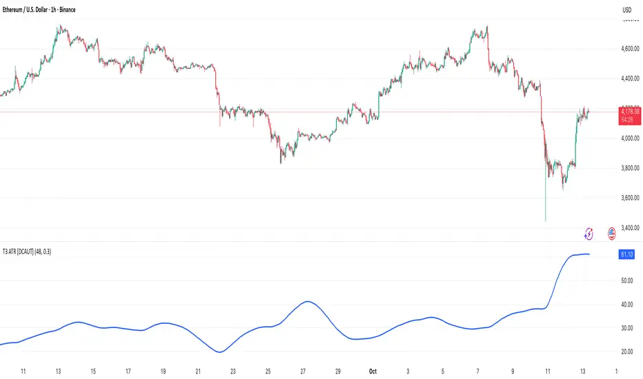
Mutanabby_AI | Fresh Algo V24Mutanabby_AI | Fresh Algo V24: Advanced Multi-Mode Trading System
Overview
The Mutanabby_AI Fresh Algo V24 represents a sophisticated evolution of multi-component trading systems that adapts to various market conditions through advanced operational configurations and enhanced analytical capabilities. This comprehensive indicator provides traders with multiple signal generation approaches, specialized assistant functions, and dynamic risk management tools designed for professional market analysis across diverse trading environments.
Primary Signal Generation Framework
The Fresh Algo V24 operates through two fundamental signal generation approaches that accommodate different market perspectives and trading philosophies. The Trending Signals Mode serves as the primary trend-following mechanism, combining Wave Trend Oscillator analysis with Supertrend directional signals and Squeeze Momentum breakout detection. This mode incorporates ADX filtering that requires values exceeding 20 to ensure sufficient trend strength exists before signal activation, making it particularly effective during sustained directional market movements where momentum persistence creates profitable trading opportunities.
The Contrarian Signals Mode provides an alternative approach targeting reversal opportunities through extreme market condition identification. This mode activates when the Wave Trend Oscillator reaches critical threshold levels, specifically when readings surpass 65 indicating potential bearish reversal conditions or drop below 35 suggesting bullish reversal opportunities. This methodology proves valuable during overextended market phases where mean reversion becomes statistically probable.
Advanced Filtering Mechanisms
The system incorporates multiple sophisticated filtering mechanisms designed to enhance signal quality and reduce false positive occurrences. The High Volume Filter requires volume expansion confirmation before signal activation, utilizing exponential moving average calculations to ensure institutional participation accompanies price movements. This filter substantially improves signal reliability by eliminating low-conviction breakouts that lack adequate volume support from professional market participants.
The Strong Filter provides additional trend confirmation through 200-period exponential moving average analysis. Long position signals require price action above this benchmark level, while short position signals necessitate price action below it. This ensures strategic alignment with longer-term trend direction and reduces the probability of trading against major market movements that could invalidate shorter-term signals.
Cloud Filter Configuration System
The Fresh Algo V24 offers four distinct cloud filter configurations, each optimized for specific trading timeframes and market approaches. The Smooth Cloud Filter utilizes the mathematical relationship between 150-period and 250-period exponential moving averages, providing stable trend identification suitable for position trading strategies. This configuration generates signals exclusively when price action aligns with cloud direction, creating a more deliberate but highly reliable signal generation process.
The Swing Cloud Filter employs modified Supertrend calculations with parameters specifically optimized for swing trading timeframes. This filter achieves optimal balance between responsiveness and stability, adapting effectively to medium-term price movements while filtering excessive market noise that typically affects shorter-term analytical systems.
For active intraday traders, the Scalping Cloud Filter utilizes accelerated Supertrend calculations designed to capture rapid trend changes effectively. This configuration provides enhanced signal generation frequency suitable for compressed timeframe strategies. The advanced Scalping+ Cloud Filter incorporates Hull Moving Average confirmation, delivering maximum responsiveness for ultra-short-term trading while maintaining signal quality through additional momentum validation processes.
Specialized Assistant Functionality
The system includes two distinct assistant modes that provide supplementary market analysis capabilities. The Trend Assistant Mode activates advanced cloud analysis overlays that display dynamic support and resistance zones calculated through adaptive volatility algorithms. These levels automatically adjust to current market conditions, providing visual guidance for identifying trend continuation patterns and potential reversal areas with mathematical precision.
The Trend Tracker Mode concentrates on long-term trend identification by displaying major exponential moving averages with color-coded fill areas that clarify directional bias. This mode maintains visual simplicity while providing comprehensive trend context evaluation, enabling traders to quickly assess broader market direction and align shorter-term strategies accordingly.
Dynamic Risk Management System
The integrated risk management system automatically adapts across all operational modes, calculating stop loss and take profit targets using Average True Range multiples that adjust to current market volatility. This approach ensures consistent risk parameters regardless of selected operational mode while maintaining relevance to prevailing market conditions.
Stop loss placement occurs at dynamically calculated distances from entry points, while three progressive take profit targets establish at customizable ATR multiples respectively. The system automatically updates these levels upon trend direction changes, ensuring current market volatility influences all risk calculations and maintains appropriate risk-reward ratios throughout trade management.
Comprehensive Market Analysis Dashboard
The sophisticated dashboard provides real-time market analysis including volatility measurements, institutional activity assessment, and multi-timeframe trend evaluation across five-minute through four-hour periods. This comprehensive market context assists traders in selecting appropriate operational modes based on current market characteristics rather than relying exclusively on historical performance data.
The multi-timeframe analysis ensures mode selection considers broader market context beyond the primary trading timeframe, improving overall strategic alignment and reducing conflicts between different temporal market perspectives. The dashboard displays market state classification, volatility percentages, institutional activity levels, current trading session information, and trend pressure indicators with professional formatting and clear visual hierarchy.
Enhanced Trading Assistants
The Fresh Algo V24 includes specialized trading assistant features that complement the primary signal generation system. The Reversal Dot functionality identifies potential reversal points through Wave Trend Oscillator analysis, displaying visual indicators when crossover conditions occur at extreme levels. These reversal indicators provide early warning signals for potential trend changes before they appear in the primary signal system.
The Dynamic Take Profit Labels feature automatically identifies optimal profit-taking opportunities through RSI threshold analysis, marking potential exit points at multiple levels for long positions and corresponding levels for short positions. This automated profit management system helps traders optimize exit timing without requiring constant manual monitoring of technical indicators.
Advanced Alert System
The comprehensive alert system accommodates all operational modes while providing granular notification control for various signal types and risk management events. Traders can configure separate alerts for normal buy signals, strong buy signals, normal sell signals, strong sell signals, stop loss triggers, and individual take profit target achievements.
Cloud crossover alerts notify traders when trend direction changes occur, providing early indication of potential strategy adjustments. The alert system includes detailed trade setup information, timeframe data, and relevant entry and exit levels, ensuring traders receive complete context for informed decision-making without requiring constant chart monitoring.
Technical Foundation Architecture
The Fresh Algo V24 combines multiple proven technical analysis components including Wave Trend Oscillator for momentum assessment, Supertrend for directional bias determination, Squeeze Momentum for volatility analysis, and various exponential moving averages for trend confirmation. Each component contributes specific market insights while the unified system provides comprehensive market evaluation through their mathematical integration.
The multi-component approach reduces dependency on individual indicator limitations while leveraging the analytical strengths of each technical tool. This creates a robust analytical framework capable of adapting to diverse market conditions through appropriate mode selection and parameter optimization, ensuring consistent performance across varying market environments.
Market State Classification
The indicator incorporates advanced market state classification through ADX analysis, distinguishing between trending, ranging, and transitional market conditions. This classification system automatically adjusts signal sensitivity and filtering parameters based on current market characteristics, optimizing performance for prevailing conditions rather than applying static analytical approaches.
The volatility measurement system calculates current market activity levels as percentages, providing quantitative assessment of market energy and helping traders select appropriate operational modes. Institutional activity detection through volume analysis ensures signal generation aligns with professional market participation patterns.
Implementation Strategy Considerations
Successful implementation requires careful matching of operational modes to prevailing market conditions and individual trading objectives. Trending modes demonstrate optimal performance during directional markets with sustained momentum characteristics, while contrarian modes excel during range-bound or overextended market conditions where reversal probability increases.
The cloud filter configurations provide varying degrees of confirmation strength, with smoother settings reducing false signal occurrence at the expense of some responsiveness to price changes. Traders must balance signal quality against signal frequency based on their risk tolerance and available trading time, utilizing the comprehensive customization options to optimize performance for their specific requirements.
Multi-Timeframe Integration
The system provides seamless multi-timeframe analysis through the integrated dashboard, displaying trend alignment across multiple time horizons from five-minute through four-hour periods. This analysis helps traders understand broader market context and avoid conflicts between different temporal perspectives that could compromise trade outcomes.
Session analysis identifies current trading session characteristics, providing context for expected market behavior patterns and helping traders adjust their approach based on typical session volatility and participation levels. This geographic market awareness enhances strategic decision-making and improves timing for trade execution.
Advanced Visualization Features
The indicator includes sophisticated visualization capabilities through gradient candle coloring based on MACD analysis, providing immediate visual feedback on momentum strength and direction. This enhancement allows rapid market assessment without requiring detailed indicator analysis, improving efficiency for traders managing multiple instruments simultaneously.
The cloud visualization system uses color-coded fill areas to clearly indicate trend direction and strength, with automatic adaptation to selected operational modes. This visual clarity reduces analytical complexity while maintaining comprehensive market information display through professional chart presentation.
Performance Optimization Framework
The Fresh Algo V24 incorporates performance optimization features including signal strength classification, automatic parameter adjustment based on market conditions, and dynamic filtering that adapts to current volatility levels. These optimizations ensure consistent performance across varying market environments while maintaining signal quality standards.
The system automatically adjusts sensitivity levels based on selected operational modes, ensuring appropriate responsiveness for different trading approaches. This adaptive framework reduces the need for manual parameter adjustments while maintaining optimal performance characteristics for each operational configuration.
Conclusion
The Mutanabby_AI Fresh Algo V24 represents a comprehensive solution for professional trading analysis, combining multiple analytical approaches with advanced visualization and risk management capabilities. The system's strength lies in its adaptive multi-mode design and sophisticated filtering mechanisms, providing traders with versatile tools for various market conditions and trading styles.
Success with this system requires understanding the relationship between different operational modes and their optimal application scenarios. The comprehensive dashboard and alert system provide essential market context and trade management support, enabling systematic approach to market analysis while maintaining flexibility for individual trading preferences.
The indicator's sophisticated architecture and extensive customization options make it suitable for traders at all experience levels, from those seeking systematic signal generation to advanced practitioners requiring comprehensive market analysis tools. The multi-timeframe integration and adaptive filtering ensure consistent performance across diverse market conditions while providing clear guidelines for strategic implementation.

Volume Footprint Anomaly Scanner [PhenLabs]📊 PhenLabs - Volume Footprint Anomaly Scanner (VFAS)
Version: PineScript™ v6
📌 Description
The PhenLabs Volume Footprint Anomaly Scanner (VFAS) is an advanced Pine Script indicator designed to detect and highlight significant imbalances in buying and selling pressure within individual price bars. By analyzing a calculated "Delta" – the net difference between estimated buy and sell volume – and employing statistical Z-score analysis, VFAS pinpoints moments when buying or selling activity becomes unusually dominant. This script was created not in hopes of creating a "Buy and Sell" indicator but rather providing the user with a more in-depth insight into the intrabar volume delta and how it can fluctuate in unusual ways, leading to anomalies that can be capitalized on.
This indicator helps traders identify high-conviction points where strong market participants are active, signaling potential shifts in momentum or continuation of a trend. It aims to provide a clearer understanding of underlying market dynamics, allowing for more informed decision-making in various trading strategies, from identifying entry points to confirming trend strength.
🚀 Points of Innovation
● Z-Score for Delta Analysis : Utilizes statistical Z-scores to objectively identify statistically significant anomalies in buying/selling pressure, moving beyond simple, arbitrary thresholds.
● Dynamic Confidence Scoring : Assigns a multi-star confidence rating (1-4 stars) to each signal, factoring in high volume, trend alignment, and specific confirmation criteria, providing a nuanced view of signal strength.
● Integrated Trend Filtering : Offers an optional Exponential Moving Average (EMA)-based trend filter to ensure signals align with the broader market direction, reducing false positives in ranging markets.
● Strict Confirmation Logic : Implements specific confirmation criteria for higher-confidence signals, including price action and a time-based gap from previous signals, enhancing reliability.
● Intuitive Info Dashboard : Provides a real-time summary of market trend and the latest signal's direction and confidence directly on the chart, streamlining information access.
🔧 Core Components
● Core Delta Engine : Estimates the net buying/selling pressure (bar Delta) by analyzing price movement within each bar relative to volume. It also calculates average volume to identify bars with unusually high activity.
● Anomaly Detection (Z-Score) : Computes the Z-score for the current bar's Delta, indicating how many standard deviations it is from its recent average. This statistical measure is central to identifying significant anomalies.
● Trend Filter : Utilizes a dual Exponential Moving Average (EMA) cross-over system to define the prevailing market trend (uptrend, downtrend, or range), providing contextual awareness.
● Signal Processing & Confidence Algorithm : Evaluates anomaly conditions against trend filters and confirmation rules, then calculates a dynamic confidence score to produce actionable, contextualized signal information.
🔥 Key Features
● Advanced Delta Anomaly Detection : Pinpoints bars with exceptionally high buying or selling pressure, indicating potential institutional activity or strong market conviction.
● Multi-Factor Confidence Scoring : Each signal comes with a 1-4 star rating, clearly communicating its reliability based on high volume, trend alignment, and specific confirmation criteria.
● Optional Trend Alignment : Users can choose to filter signals, so only those aligned with the prevailing EMA-defined trend are displayed, enhancing signal quality.
● Interactive Signal Labels : Displays compact labels on the chart at anomaly points, offering detailed tooltips upon hover, including signal type, direction, confidence, and contextual information.
● Customizable Bar Colors : Visually highlights bars with Delta anomalies, providing an immediate visual cue for strong buying or selling activity.
● Real-time Info Dashboard : A clean, customizable dashboard shows the current market trend and details of the latest detected signal, keeping key information accessible at a glance.
● Configurable Alerts : Set up alerts for bullish or bearish Delta anomalies to receive real-time notifications when significant market pressure shifts occur.
🎨 Visualization
Signal Labels :
* Placed at the top/bottom of anomaly bars, showing a "📈" (bullish) or "📉" (bearish) icon.
* Tooltip: Hovering over a label reveals detailed information: Signal Type (e.g., "Delta Anomaly"), Direction, Confidence (e.g., "★★★☆"), and a descriptive explanation of the anomaly.
* Interpretation: Clearly marks actionable signals and provides deep insights without cluttering the chart, enabling quick assessment of signal strength and context.
● Info Dashboard :
* Located at the top-right of the chart, providing a clean summary.
* Displays: "PhenLabs - VFAS" header, "Market Trend" (Uptrend/Downtrend/Range with color-coded status), and "Direction | Conf." (showing the last signal's direction and star confidence).
* Optional "💡 Hover over signals for details" reminder.
* Interpretation: A concise, real-time summary of the market's pulse and the most recent high-conviction event, helping traders stay informed at a glance.
📖 Usage Guidelines
Setting Categories
⚙️ Core Delta & Volume Engine
● Minimum Volume Lookback (Bars)
○ Default: 9
○ Range: Integer (e.g., 5-50)
○ Description: Defines the number of preceding bars used to calculate the average volume and delta. Bars with volume below this average won't be considered for high-volume signals. A shorter lookback is more reactive to recent changes, while a longer one provides a smoother average.
📈 Anomaly Detection Settings
Delta Z-Score Anomaly Threshold
○ Default: 2.5
○ Range: Float (e.g., 1.0-5.0+)
○ Description: The number of standard deviations from the mean that a bar's delta must exceed to be considered a significant anomaly. A higher threshold means fewer, but potentially stronger, signals. A lower threshold will generate more signals, which might include less significant events. Experiment to find the optimal balance for your trading style.
🔬 Context Filters
Enable Trend Filter
○ Default: False
○ Range: Boolean (True/False)
○ Description: When enabled, signals will only be generated if they align with the current market trend as determined by the EMAs (e.g., only bullish signals in an uptrend, bearish in a downtrend). This helps to filter out counter-trend noise.
● Trend EMA Fast
○ Default: 50
○ Range: Integer (e.g., 10-100)
○ Description: The period for the faster Exponential Moving Average used in the trend filter. In combination with the slow EMA, it defines the trend direction.
● Trend EMA Slow
○ Default: 200
○ Range: Integer (e.g., 100-400)
○ Description: The period for the slower Exponential Moving Average used in the trend filter. The relationship between the fast and slow EMA determines if the market is in an uptrend (fast > slow) or downtrend (fast < slow).
🎨 Visual & UI Settings
● Show Info Dashboard
○ Default: True
○ Range: Boolean (True/False)
○ Description: Toggles the visibility of the dashboard on the chart, which provides a summary of market trend and the last detected signal.
● Show Dashboard Tooltip
○ Default: True
○ Range: Boolean (True/False)
○ Description: Toggles a reminder message in the dashboard to hover over signal labels for more detailed information.
● Show Delta Anomaly Bar Colors
○ Default: True
○ Range: Boolean (True/False)
○ Description: Enables or disables the coloring of bars based on their delta direction and whether they represent a significant anomaly.
● Show Signal Labels
○ Default: True
○ Range: Boolean (True/False)
○ Description: Controls the visibility of the “📈” or “📉” labels that appear on the chart when a delta anomaly signal is generated.
🔔 Alert Settings
Alert on Delta Anomaly
○ Default: True
○ Range: Boolean (True/False)
○ Description: When enabled, this setting allows you to set up alerts in TradingView that will trigger whenever a new bullish or bearish delta anomaly is detected.
✅ Best Use Cases
Early Trend Reversal / Continuation Detection: Identify strong surges of buying/selling pressure at key support/resistance levels that could indicate a reversal or the continuation of a strong move.
● Confirmation of Breakouts: Use high-confidence delta anomalies to confirm the validity of price breakouts, indicating strong conviction behind the move.
● Entry and Exit Points: Pinpoint precise entry opportunities when anomalies align with your trading strategy, or identify potential exhaustion signals for exiting trades.
● Scalping and Day Trading: The indicator’s sensitivity to intraday buying/selling imbalances makes it highly effective for short-term trading strategies.
● Market Sentiment Analysis: Gain a real-time understanding of underlying market sentiment by observing the prevalence and strength of bullish vs. bearish anomalies.
⚠️ Limitations
Estimated Delta: The script uses a simplified method to estimate delta based on bar close relative to its range, not actual order book or footprint data. While effective, it’s an approximation.
● Sensitivity to Z-Score Threshold: The effectiveness heavily relies on the `Delta Z-Score Anomaly Threshold`. Too low, and you’ll get many false positives; too high, and you might miss valid signals.
● Confirmation Criteria: The 4-star confidence level’s “confirmation” relies on specific subsequent bar conditions and previous confirmed signals, which might be too strict or specific for all contexts.
● Requires Context: While powerful, VFAS is best used in conjunction with other technical analysis tools and price action to form a comprehensive trading strategy. It is not a standalone “buy/sell” signal.
💡 What Makes This Unique
Statistical Rigor: The application of Z-score analysis to bar delta provides an objective, statistically-driven way to identify true anomalies, moving beyond arbitrary thresholds.
● Multi-Factor Confidence Scoring: The unique 1-4 star confidence system integrates multiple market dynamics (volume, trend alignment, specific follow-through) into a single, easy-to-interpret rating.
● User-Friendly Design: From the intuitive dashboard to the detailed signal tooltips, the indicator prioritizes clear and accessible information for traders of all experience levels.
🔬 How It Works
1. Bar Delta Calculation:
● The script first estimates the “buy volume” and “sell volume” for each bar. This is done by assuming that volume proportional to the distance from the low to the close represents buying, and volume proportional to the distance from the high to the close represents selling.
● How this contributes: This provides a proxy for the net buying or selling pressure (delta) within that specific price bar, even without access to actual footprint data.
2. Volume & Delta Z-Score Analysis:
● The average volume over a user-defined lookback period is calculated. Bars with volume less than twice this average are generally considered of lower interest.
● The Z-score for the calculated bar delta is computed. The Z-score measures how many standard deviations the current bar’s delta is from its average delta over the `Minimum Volume Lookback` period.
● How this contributes: A high positive Z-score indicates a bullish delta anomaly (significantly more buying than usual), while a high negative Z-score indicates a bearish delta anomaly (significantly more selling than usual). This identifies statistically unusual levels of pressure.
3. Trend Filtering (Optional):
● Two Exponential Moving Averages (Fast and Slow EMA) are used to determine the prevailing market trend. An uptrend is identified when the Fast EMA is above the Slow EMA, and a downtrend when the Fast EMA is below the Slow EMA.
● How this contributes: If enabled, the indicator will only display bullish delta anomalies during an uptrend and bearish delta anomalies during a downtrend, helping to confirm signals within the broader market context and avoid counter-trend signals.
4. Signal Generation & Confidence Scoring:
● When a delta Z-score exceeds the user-defined anomaly threshold, a signal is generated.
● This signal is then passed through a multi-factor confidence algorithm (`f_calculateConfidence`). It awards stars based on: high volume presence, alignment with the overall trend (if enabled), and a fourth star for very strong Z-scores (above 3.0) combined with specific follow-through candle patterns after a cooling-off period from a previous confirmed signal.
● How this contributes: Provides a qualitative rating (1-4 stars) for each anomaly, allowing traders to quickly assess the potential significance and reliability of the signal.
💡 Note:
The PhenLabs Volume Footprint Anomaly Scanner is a powerful analytical tool, but it’s crucial to understand that no indicator guarantees profit. Always backtest and forward-test the indicator settings on your chosen assets and timeframes. Consider integrating VFAS with your existing trading strategy, using its signals as confirmation for entries, exits, or trend bias. The Z-score threshold is highly customizable; lower values will yield more signals (including potential noise), while higher values will provide fewer but potentially higher-conviction signals. Adjust this parameter based on market volatility and your risk tolerance. Remember to combine statistical insights from VFAS with price action, support/resistance levels, and your overall market outlook for optimal results.
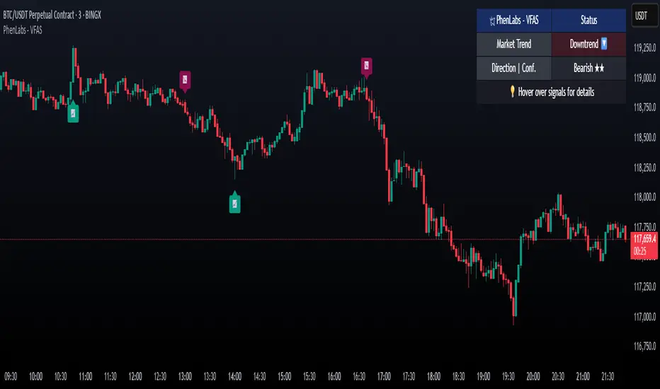
BACAP PRICE STRUCTURE 21 EMA TREND21dma-STRUCTURE
Overview
The 21dma-STRUCTURE indicator is a sophisticated overlay indicator that visualizes price action relative to a triple 21-period exponential moving average structure. Originally developed by BalarezoCapital and enhanced by PrimeTrading, this indicator provides clear visual cues for trend direction and momentum through dynamic bar coloring and EMA structure analysis.
Key Features
Triple EMA Structure
- 21 EMA High: Tracks the exponential moving average of high prices
- 21 EMA Close: Tracks the exponential moving average of closing prices
- 21 EMA Low: Tracks the exponential moving average of low prices
- Dynamic Cloud: Gray fill between high and low EMAs for visual structure reference
Smart Bar Coloring System
- Blue Bars: Price closes above all three EMAs (strong bullish momentum)
- Pink Bars: Daily high falls below the lowest EMA (strong bearish signal)
- Gray Bars: Neutral conditions or transitional phases
- Color Memory: Maintains previous color until new condition is met
Dynamic Center Line
- Trend-Following Color: Green when all EMAs are rising, red when all are falling
- Color Persistence: Maintains trend color during sideways movement
- Visual Clarity: Thicker center line for easy trend identification
Customizable Visual Elements
- Adjustable line thickness for all EMA plots
- Customizable colors for bullish and bearish conditions
- Configurable trend colors for uptrend and downtrend phases
- Optional bar color changes with toggle control
How to Use
Trend Identification
- Rising Green Center Line: All EMAs trending upward (bullish structure)
- Falling Red Center Line: All EMAs trending downward (bearish structure)
- Flat Center Line: Maintains last trend color during consolidation
Momentum Analysis
- Blue Bars: Strong bullish momentum with price above entire EMA structure
- Pink Bars: Strong bearish momentum with high below lowest EMA
- Gray Bars: Neutral or transitional momentum phases
Entry and Exit Signals
- Bullish Setup: Look for blue bars during green center line periods
- Bearish Setup: Look for pink bars during red center line periods
- Exit Consideration: Watch for color changes as potential momentum shifts
Structure Trading
- Support/Resistance: Use EMA cloud as dynamic support and resistance zones
- Breakout Confirmation: Bar color changes can confirm structure breakouts
- Trend Continuation: Color persistence suggests ongoing momentum
Settings
Visual Customization
- Change Bar Color: Toggle to enable/disable bar coloring
- Line Size: Adjust thickness of EMA lines (default: 3)
- Bullish Candle Color: Customize blue bar color
- Bearish Candle Color: Customize pink bar color
Trend Colors
- Uptrend Color: Color for rising EMA center line (default: green)
- Downtrend Color: Color for falling EMA center line (default: red)
- Cloud Color: Fill color between high and low EMAs (default: gray)
Advanced Features
Modified Bar Logic
Unlike traditional EMA systems, this indicator uses refined conditions:
- Bullish signals require close above ALL three EMAs
- Bearish signals require high below the LOWEST EMA
- Enhanced precision reduces false signals compared to single EMA systems
Trend Memory System
- Intelligent color persistence during sideways movement
- Reduces noise from minor EMA fluctuations
- Maintains trend context during consolidation periods
Performance Optimization
- Efficient calculation methods for real-time performance
- Clean visual design that doesn't clutter charts
- Compatible with all timeframes and instruments
Best Practices
Multi-Timeframe Analysis
- Use higher timeframes to identify overall trend direction
- Apply on multiple timeframes for confluence
- Combine with weekly/monthly charts for position trading
Risk Management
- Use bar color changes as early warning signals
- Consider position sizing based on EMA structure strength
- Set stops relative to EMA support/resistance levels
Combination Strategies
- Pair with volume indicators for confirmation
- Use alongside RSI or MACD for momentum confirmation
- Combine with key support/resistance levels
Market Context
- More effective in trending markets than choppy conditions
- Consider overall market environment and sector strength
- Adjust expectations during high volatility periods
Technical Specifications
- Based on 21-period exponential moving averages
- Uses Pine Script v6 for optimal performance
- Overlay indicator that works with any chart type
- Maximum 500 lines for clean performance
Ideal Applications
- Swing trading on daily charts
- Position trading on weekly charts
- Intraday momentum trading (adjust timeframe accordingly)
- Trend following strategies
- Structure-based trading approaches
Disclaimer
This indicator is for educational and informational purposes only. It should not be used as the sole basis for trading decisions. Always combine with other forms of analysis, proper risk management, and consider your individual trading plan and risk tolerance.
Compatible with Pine Script v6 | Works on all timeframes | Optimized for trending markets
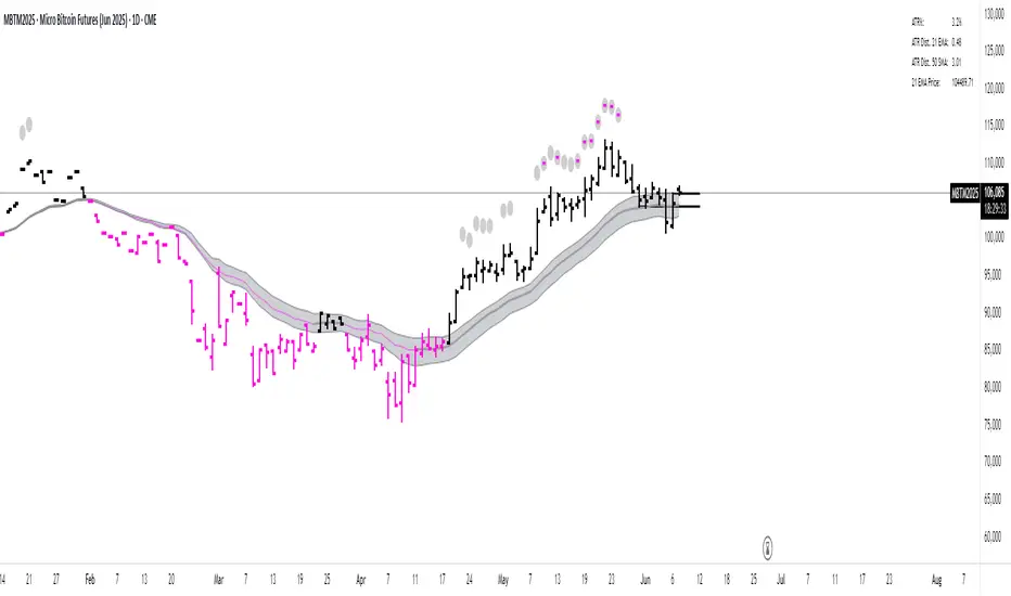
Kernel Weighted DMI | QuantEdgeB📊 Introducing Kernel Weighted DMI (K-DMI) by QuantEdgeB
🛠️ Overview
K-DMI is a next-gen momentum indicator that combines the traditional Directional Movement Index (DMI) with advanced kernel smoothing techniques to produce a highly adaptive, noise-resistant trend signal.
Unlike standard DMI that can be overly reactive or choppy in consolidation phases, K-DMI applies kernel-weighted filtering (Linear, Exponential, or Gaussian) to stabilize directional movement readings and extract a more reliable momentum signal.
✨ Key Features
🔹 Kernel Smoothing Engine
Smooths DMI using your choice of kernel (Linear, Exponential, Gaussian) for flexible noise reduction and clarity.
🔹 Dynamic Trend Signal
Generates real-time long/short trend bias based on signal crossing upper or lower thresholds (defaults: ±1).
🔹 Visual Encoding
Includes directional gradient fills, candle coloring, and momentum-based overlays for instant signal comprehension.
🔹 Multi-Mode Plotting
Optional moving average overlays visualize structure and compression/expansion within price action.
📐 How It Works
1️⃣ Directional Movement Index (DMI)
Calculates the traditional +DI and -DI differential to derive directional bias.
2️⃣ Kernel-Based Smoothing
Applies a custom-weighted average across historical DMI values using one of three smoothing methods:
• Linear → Simple tapering weights
• Exponential → Decay curve for recent emphasis
• Gaussian → Bell-shaped weight for centered precision
3️⃣ Signal Generation
• ✅ Long → Signal > Long Threshold (default: +1)
• ❌ Short → Signal < Short Threshold (default: -1)
Additional overlays signal potential compression zones or trend resumption using gradient and line fills.
⚙️ Custom Settings
• DMI Length: Default = 7
• Kernel Type: Options → Linear, Exponential, Gaussian (Def:Linear)
• Kernel Length: Default = 25
• Long Threshold: Default = 1
• Short Threshold: Default = -1
• Color Mode: Strategy, Solar, Warm, Cool, Classic, Magic
• Show Labels: Optional entry signal labels (Long/Short)
• Enable Extra Plots: Toggle MA overlays and dynamic bands
👥 Who Is It For?
✅ Trend Traders → Identify sustained directional bias with smoother signal lines
✅ Quant Analysts → Leverage advanced smoothing models to enhance data clarity
✅ Discretionary Swing Traders → Visualize clean breakouts or fades within choppy zones
✅ MA Compression Traders → Use overlay MAs to detect expansion opportunities
📌 Conclusion
Kernel Weighted DMI is the evolution of classic momentum tracking—merging traditional DMI logic with adaptable kernel filters. It provides a refined lens for trend detection, while optional visual overlays support price structure analysis.
🔹 Key Takeaways:
1️⃣ Smoothed and stabilized DMI for reliable trend signal generation
2️⃣ Optional Gaussian/exponential weighting for adaptive responsiveness
3️⃣ Custom gradient fills, dynamic MAs, and candle coloring to support visual clarity
📌 Disclaimer: Past performance is not indicative of future results. No trading strategy can guarantee success in financial markets.
📌 Strategic Advice: Always backtest, optimize, and align parameters with your trading objectives and risk tolerance before live trading.

real_time_candlesIntroduction
The Real-Time Candles Library provides comprehensive tools for creating, manipulating, and visualizing custom timeframe candles in Pine Script. Unlike standard indicators that only update at bar close, this library enables real-time visualization of price action and indicators within the current bar, offering traders unprecedented insight into market dynamics as they unfold.
This library addresses a fundamental limitation in traditional technical analysis: the inability to see how indicators evolve between bar closes. By implementing sophisticated real-time data processing techniques, traders can now observe indicator movements, divergences, and trend changes as they develop, potentially identifying trading opportunities much earlier than with conventional approaches.
Key Features
The library supports two primary candle generation approaches:
Chart-Time Candles: Generate real-time OHLC data for any variable (like RSI, MACD, etc.) while maintaining synchronization with chart bars.
Custom Timeframe (CTF) Candles: Create candles with custom time intervals or tick counts completely independent of the chart's native timeframe.
Both approaches support traditional candlestick and Heikin-Ashi visualization styles, with options for moving average overlays to smooth the data.
Configuration Requirements
For optimal performance with this library:
Set max_bars_back = 5000 in your script settings
When using CTF drawing functions, set max_lines_count = 500, max_boxes_count = 500, and max_labels_count = 500
These settings ensure that you will be able to draw correctly and will avoid any runtime errors.
Usage Examples
Basic Chart-Time Candle Visualization
// Create real-time candles for RSI
float rsi = ta.rsi(close, 14)
Candle rsi_candle = candle_series(rsi, CandleType.candlestick)
// Plot the candles using Pine's built-in function
plotcandle(rsi_candle.Open, rsi_candle.High, rsi_candle.Low, rsi_candle.Close,
"RSI Candles", rsi_candle.candle_color, rsi_candle.candle_color)
Multiple Access Patterns
The library provides three ways to access candle data, accommodating different programming styles:
// 1. Array-based access for collection operations
Candle candles = candle_array(source)
// 2. Object-oriented access for single entity manipulation
Candle candle = candle_series(source)
float value = candle.source(Source.HLC3)
// 3. Tuple-based access for functional programming styles
= candle_tuple(source)
Custom Timeframe Examples
// Create 20-second candles with EMA overlay
plot_ctf_candles(
source = close,
candle_type = CandleType.candlestick,
sample_type = SampleType.Time,
number_of_seconds = 20,
timezone = -5,
tied_open = true,
ema_period = 9,
enable_ema = true
)
// Create tick-based candles (new candle every 15 ticks)
plot_ctf_tick_candles(
source = close,
candle_type = CandleType.heikin_ashi,
number_of_ticks = 15,
timezone = -5,
tied_open = true
)
Advanced Usage with Custom Visualization
// Get custom timeframe candles without automatic plotting
CandleCTF my_candles = ctf_candles_array(
source = close,
candle_type = CandleType.candlestick,
sample_type = SampleType.Time,
number_of_seconds = 30
)
// Apply custom logic to the candles
float ema_values = my_candles.ctf_ema(14)
// Draw candles and EMA using time-based coordinates
my_candles.draw_ctf_candles_time()
ema_values.draw_ctf_line_time(line_color = #FF6D00)
Library Components
Data Types
Candle: Structure representing chart-time candles with OHLC, polarity, and visualization properties
CandleCTF: Extended candle structure with additional time metadata for custom timeframes
TickData: Structure for individual price updates with time deltas
Enumerations
CandleType: Specifies visualization style (candlestick or Heikin-Ashi)
Source: Defines price components for calculations (Open, High, Low, Close, HL2, etc.)
SampleType: Sets sampling method (Time-based or Tick-based)
Core Functions
get_tick(): Captures current price as a tick data point
candle_array(): Creates an array of candles from price updates
candle_series(): Provides a single candle based on latest data
candle_tuple(): Returns OHLC values as a tuple
ctf_candles_array(): Creates custom timeframe candles without rendering
Visualization Functions
source(): Extracts specific price components from candles
candle_ctf_to_float(): Converts candle data to float arrays
ctf_ema(): Calculates exponential moving averages for candle arrays
draw_ctf_candles_time(): Renders candles using time coordinates
draw_ctf_candles_index(): Renders candles using bar index coordinates
draw_ctf_line_time(): Renders lines using time coordinates
draw_ctf_line_index(): Renders lines using bar index coordinates
Technical Implementation Notes
This library leverages Pine Script's varip variables for state management, creating a sophisticated real-time data processing system. The implementation includes:
Efficient tick capturing: Samples price at every execution, maintaining temporal tracking with time deltas
Smart state management: Uses a hybrid approach with mutable updates at index 0 and historical preservation at index 1+
Temporal synchronization: Manages two time domains (chart time and custom timeframe)
The tooltip implementation provides crucial temporal context for custom timeframe visualizations, allowing users to understand exactly when each candle formed regardless of chart timeframe.
Limitations
Custom timeframe candles cannot be backtested due to Pine Script's limitations with historical tick data
Real-time visualization is only available during live chart updates
Maximum history is constrained by Pine Script's array size limits
Applications
Indicator visualization: See how RSI, MACD, or other indicators evolve in real-time
Volume analysis: Create custom volume profiles independent of chart timeframe
Scalping strategies: Identify short-term patterns with precisely defined time windows
Volatility measurement: Track price movement characteristics within bars
Custom signal generation: Create entry/exit signals based on custom timeframe patterns
Conclusion
The Real-Time Candles Library bridges the gap between traditional technical analysis (based on discrete OHLC bars) and the continuous nature of market movement. By making indicators more responsive to real-time price action, it gives traders a significant edge in timing and decision-making, particularly in fast-moving markets where waiting for bar close could mean missing important opportunities.
Whether you're building custom indicators, researching price patterns, or developing trading strategies, this library provides the foundation for sophisticated real-time analysis in Pine Script.
Implementation Details & Advanced Guide
Core Implementation Concepts
The Real-Time Candles Library implements a sophisticated event-driven architecture within Pine Script's constraints. At its heart, the library creates what's essentially a reactive programming framework handling continuous data streams.
Tick Processing System
The foundation of the library is the get_tick() function, which captures price updates as they occur:
export get_tick(series float source = close, series float na_replace = na)=>
varip float price = na
varip int series_index = -1
varip int old_time = 0
varip int new_time = na
varip float time_delta = 0
// ...
This function:
Samples the current price
Calculates time elapsed since last update
Maintains a sequential index to track updates
The resulting TickData structure serves as the fundamental building block for all candle generation.
State Management Architecture
The library employs a sophisticated state management system using varip variables, which persist across executions within the same bar. This creates a hybrid programming paradigm that's different from standard Pine Script's bar-by-bar model.
For chart-time candles, the core state transition logic is:
// Real-time update of current candle
candle_data := Candle.new(Open, High, Low, Close, polarity, series_index, candle_color)
candles.set(0, candle_data)
// When a new bar starts, preserve the previous candle
if clear_state
candles.insert(1, candle_data)
price.clear()
// Reset state for new candle
Open := Close
price.push(Open)
series_index += 1
This pattern of updating index 0 in real-time while inserting completed candles at index 1 creates an elegant solution for maintaining both current state and historical data.
Custom Timeframe Implementation
The custom timeframe system manages its own time boundaries independent of chart bars:
bool clear_state = switch settings.sample_type
SampleType.Ticks => cumulative_series_idx >= settings.number_of_ticks
SampleType.Time => cumulative_time_delta >= settings.number_of_seconds
This dual-clock system synchronizes two time domains:
Pine's execution clock (bar-by-bar processing)
The custom timeframe clock (tick or time-based)
The library carefully handles temporal discontinuities, ensuring candle formation remains accurate despite irregular tick arrival or market gaps.
Advanced Usage Techniques
1. Creating Custom Indicators with Real-Time Candles
To develop indicators that process real-time data within the current bar:
// Get real-time candles for your data
Candle rsi_candles = candle_array(ta.rsi(close, 14))
// Calculate indicator values based on candle properties
float signal = ta.ema(rsi_candles.first().source(Source.Close), 9)
// Detect patterns that occur within the bar
bool divergence = close > close and rsi_candles.first().Close < rsi_candles.get(1).Close
2. Working with Custom Timeframes and Plotting
For maximum flexibility when visualizing custom timeframe data:
// Create custom timeframe candles
CandleCTF volume_candles = ctf_candles_array(
source = volume,
candle_type = CandleType.candlestick,
sample_type = SampleType.Time,
number_of_seconds = 60
)
// Convert specific candle properties to float arrays
float volume_closes = volume_candles.candle_ctf_to_float(Source.Close)
// Calculate derived values
float volume_ema = volume_candles.ctf_ema(14)
// Create custom visualization
volume_candles.draw_ctf_candles_time()
volume_ema.draw_ctf_line_time(line_color = color.orange)
3. Creating Hybrid Timeframe Analysis
One powerful application is comparing indicators across multiple timeframes:
// Standard chart timeframe RSI
float chart_rsi = ta.rsi(close, 14)
// Custom 5-second timeframe RSI
CandleCTF ctf_candles = ctf_candles_array(
source = close,
candle_type = CandleType.candlestick,
sample_type = SampleType.Time,
number_of_seconds = 5
)
float fast_rsi_array = ctf_candles.candle_ctf_to_float(Source.Close)
float fast_rsi = fast_rsi_array.first()
// Generate signals based on divergence between timeframes
bool entry_signal = chart_rsi < 30 and fast_rsi > fast_rsi_array.get(1)
Final Notes
This library represents an advanced implementation of real-time data processing within Pine Script's constraints. By creating a reactive programming framework for handling continuous data streams, it enables sophisticated analysis typically only available in dedicated trading platforms.
The design principles employed—including state management, temporal processing, and object-oriented architecture—can serve as patterns for other advanced Pine Script development beyond this specific application.
------------------------
Library "real_time_candles"
A comprehensive library for creating real-time candles with customizable timeframes and sampling methods.
Supports both chart-time and custom-time candles with options for candlestick and Heikin-Ashi visualization.
Allows for tick-based or time-based sampling with moving average overlay capabilities.
get_tick(source, na_replace)
Captures the current price as a tick data point
Parameters:
source (float) : Optional - Price source to sample (defaults to close)
na_replace (float) : Optional - Value to use when source is na
Returns: TickData structure containing price, time since last update, and sequential index
candle_array(source, candle_type, sync_start, bullish_color, bearish_color)
Creates an array of candles based on price updates
Parameters:
source (float) : Optional - Price source to sample (defaults to close)
candle_type (simple CandleType) : Optional - Type of candle chart to create (candlestick or Heikin-Ashi)
sync_start (simple bool) : Optional - Whether to synchronize with the start of a new bar
bullish_color (color) : Optional - Color for bullish candles
bearish_color (color) : Optional - Color for bearish candles
Returns: Array of Candle objects ordered with most recent at index 0
candle_series(source, candle_type, wait_for_sync, bullish_color, bearish_color)
Provides a single candle based on the latest price data
Parameters:
source (float) : Optional - Price source to sample (defaults to close)
candle_type (simple CandleType) : Optional - Type of candle chart to create (candlestick or Heikin-Ashi)
wait_for_sync (simple bool) : Optional - Whether to wait for a new bar before starting
bullish_color (color) : Optional - Color for bullish candles
bearish_color (color) : Optional - Color for bearish candles
Returns: A single Candle object representing the current state
candle_tuple(source, candle_type, wait_for_sync, bullish_color, bearish_color)
Provides candle data as a tuple of OHLC values
Parameters:
source (float) : Optional - Price source to sample (defaults to close)
candle_type (simple CandleType) : Optional - Type of candle chart to create (candlestick or Heikin-Ashi)
wait_for_sync (simple bool) : Optional - Whether to wait for a new bar before starting
bullish_color (color) : Optional - Color for bullish candles
bearish_color (color) : Optional - Color for bearish candles
Returns: Tuple representing current candle values
method source(self, source, na_replace)
Extracts a specific price component from a Candle
Namespace types: Candle
Parameters:
self (Candle)
source (series Source) : Type of price data to extract (Open, High, Low, Close, or composite values)
na_replace (float) : Optional - Value to use when source value is na
Returns: The requested price value from the candle
method source(self, source)
Extracts a specific price component from a CandleCTF
Namespace types: CandleCTF
Parameters:
self (CandleCTF)
source (simple Source) : Type of price data to extract (Open, High, Low, Close, or composite values)
Returns: The requested price value from the candle as a varip
method candle_ctf_to_float(self, source)
Converts a specific price component from each CandleCTF to a float array
Namespace types: array
Parameters:
self (array)
source (simple Source) : Optional - Type of price data to extract (defaults to Close)
Returns: Array of float values extracted from the candles, ordered with most recent at index 0
method ctf_ema(self, ema_period)
Calculates an Exponential Moving Average for a CandleCTF array
Namespace types: array
Parameters:
self (array)
ema_period (simple float) : Period for the EMA calculation
Returns: Array of float values representing the EMA of the candle data, ordered with most recent at index 0
method draw_ctf_candles_time(self, sample_type, number_of_ticks, number_of_seconds, timezone)
Renders custom timeframe candles using bar time coordinates
Namespace types: array
Parameters:
self (array)
sample_type (simple SampleType) : Optional - Method for sampling data (Time or Ticks), used for tooltips
number_of_ticks (simple int) : Optional - Number of ticks per candle (used when sample_type is Ticks), used for tooltips
number_of_seconds (simple float) : Optional - Time duration per candle in seconds (used when sample_type is Time), used for tooltips
timezone (simple int) : Optional - Timezone offset from UTC (-12 to +12), used for tooltips
Returns: void - Renders candles on the chart using time-based x-coordinates
method draw_ctf_candles_index(self, sample_type, number_of_ticks, number_of_seconds, timezone)
Renders custom timeframe candles using bar index coordinates
Namespace types: array
Parameters:
self (array)
sample_type (simple SampleType) : Optional - Method for sampling data (Time or Ticks), used for tooltips
number_of_ticks (simple int) : Optional - Number of ticks per candle (used when sample_type is Ticks), used for tooltips
number_of_seconds (simple float) : Optional - Time duration per candle in seconds (used when sample_type is Time), used for tooltips
timezone (simple int) : Optional - Timezone offset from UTC (-12 to +12), used for tooltips
Returns: void - Renders candles on the chart using index-based x-coordinates
method draw_ctf_line_time(self, source, line_size, line_color)
Renders a line representing a price component from the candles using time coordinates
Namespace types: array
Parameters:
self (array)
source (simple Source) : Optional - Type of price data to extract (defaults to Close)
line_size (simple int) : Optional - Width of the line
line_color (simple color) : Optional - Color of the line
Returns: void - Renders a connected line on the chart using time-based x-coordinates
method draw_ctf_line_time(self, line_size, line_color)
Renders a line from a varip float array using time coordinates
Namespace types: array
Parameters:
self (array)
line_size (simple int) : Optional - Width of the line, defaults to 2
line_color (simple color) : Optional - Color of the line
Returns: void - Renders a connected line on the chart using time-based x-coordinates
method draw_ctf_line_index(self, source, line_size, line_color)
Renders a line representing a price component from the candles using index coordinates
Namespace types: array
Parameters:
self (array)
source (simple Source) : Optional - Type of price data to extract (defaults to Close)
line_size (simple int) : Optional - Width of the line
line_color (simple color) : Optional - Color of the line
Returns: void - Renders a connected line on the chart using index-based x-coordinates
method draw_ctf_line_index(self, line_size, line_color)
Renders a line from a varip float array using index coordinates
Namespace types: array
Parameters:
self (array)
line_size (simple int) : Optional - Width of the line, defaults to 2
line_color (simple color) : Optional - Color of the line
Returns: void - Renders a connected line on the chart using index-based x-coordinates
plot_ctf_tick_candles(source, candle_type, number_of_ticks, timezone, tied_open, ema_period, bullish_color, bearish_color, line_width, ema_color, use_time_indexing)
Plots tick-based candles with moving average
Parameters:
source (float) : Input price source to sample
candle_type (simple CandleType) : Type of candle chart to display
number_of_ticks (simple int) : Number of ticks per candle
timezone (simple int) : Timezone offset from UTC (-12 to +12)
tied_open (simple bool) : Whether to tie open price to close of previous candle
ema_period (simple float) : Period for the exponential moving average
bullish_color (color) : Optional - Color for bullish candles
bearish_color (color) : Optional - Color for bearish candles
line_width (simple int) : Optional - Width of the moving average line, defaults to 2
ema_color (color) : Optional - Color of the moving average line
use_time_indexing (simple bool) : Optional - When true the function will plot with xloc.time, when false it will plot using xloc.bar_index
Returns: void - Creates visual candle chart with EMA overlay
plot_ctf_tick_candles(source, candle_type, number_of_ticks, timezone, tied_open, bullish_color, bearish_color, use_time_indexing)
Plots tick-based candles without moving average
Parameters:
source (float) : Input price source to sample
candle_type (simple CandleType) : Type of candle chart to display
number_of_ticks (simple int) : Number of ticks per candle
timezone (simple int) : Timezone offset from UTC (-12 to +12)
tied_open (simple bool) : Whether to tie open price to close of previous candle
bullish_color (color) : Optional - Color for bullish candles
bearish_color (color) : Optional - Color for bearish candles
use_time_indexing (simple bool) : Optional - When true the function will plot with xloc.time, when false it will plot using xloc.bar_index
Returns: void - Creates visual candle chart without moving average
plot_ctf_time_candles(source, candle_type, number_of_seconds, timezone, tied_open, ema_period, bullish_color, bearish_color, line_width, ema_color, use_time_indexing)
Plots time-based candles with moving average
Parameters:
source (float) : Input price source to sample
candle_type (simple CandleType) : Type of candle chart to display
number_of_seconds (simple float) : Time duration per candle in seconds
timezone (simple int) : Timezone offset from UTC (-12 to +12)
tied_open (simple bool) : Whether to tie open price to close of previous candle
ema_period (simple float) : Period for the exponential moving average
bullish_color (color) : Optional - Color for bullish candles
bearish_color (color) : Optional - Color for bearish candles
line_width (simple int) : Optional - Width of the moving average line, defaults to 2
ema_color (color) : Optional - Color of the moving average line
use_time_indexing (simple bool) : Optional - When true the function will plot with xloc.time, when false it will plot using xloc.bar_index
Returns: void - Creates visual candle chart with EMA overlay
plot_ctf_time_candles(source, candle_type, number_of_seconds, timezone, tied_open, bullish_color, bearish_color, use_time_indexing)
Plots time-based candles without moving average
Parameters:
source (float) : Input price source to sample
candle_type (simple CandleType) : Type of candle chart to display
number_of_seconds (simple float) : Time duration per candle in seconds
timezone (simple int) : Timezone offset from UTC (-12 to +12)
tied_open (simple bool) : Whether to tie open price to close of previous candle
bullish_color (color) : Optional - Color for bullish candles
bearish_color (color) : Optional - Color for bearish candles
use_time_indexing (simple bool) : Optional - When true the function will plot with xloc.time, when false it will plot using xloc.bar_index
Returns: void - Creates visual candle chart without moving average
plot_ctf_candles(source, candle_type, sample_type, number_of_ticks, number_of_seconds, timezone, tied_open, ema_period, bullish_color, bearish_color, enable_ema, line_width, ema_color, use_time_indexing)
Unified function for plotting candles with comprehensive options
Parameters:
source (float) : Input price source to sample
candle_type (simple CandleType) : Optional - Type of candle chart to display
sample_type (simple SampleType) : Optional - Method for sampling data (Time or Ticks)
number_of_ticks (simple int) : Optional - Number of ticks per candle (used when sample_type is Ticks)
number_of_seconds (simple float) : Optional - Time duration per candle in seconds (used when sample_type is Time)
timezone (simple int) : Optional - Timezone offset from UTC (-12 to +12)
tied_open (simple bool) : Optional - Whether to tie open price to close of previous candle
ema_period (simple float) : Optional - Period for the exponential moving average
bullish_color (color) : Optional - Color for bullish candles
bearish_color (color) : Optional - Color for bearish candles
enable_ema (bool) : Optional - Whether to display the EMA overlay
line_width (simple int) : Optional - Width of the moving average line, defaults to 2
ema_color (color) : Optional - Color of the moving average line
use_time_indexing (simple bool) : Optional - When true the function will plot with xloc.time, when false it will plot using xloc.bar_index
Returns: void - Creates visual candle chart with optional EMA overlay
ctf_candles_array(source, candle_type, sample_type, number_of_ticks, number_of_seconds, tied_open, bullish_color, bearish_color)
Creates an array of custom timeframe candles without rendering them
Parameters:
source (float) : Input price source to sample
candle_type (simple CandleType) : Type of candle chart to create (candlestick or Heikin-Ashi)
sample_type (simple SampleType) : Method for sampling data (Time or Ticks)
number_of_ticks (simple int) : Optional - Number of ticks per candle (used when sample_type is Ticks)
number_of_seconds (simple float) : Optional - Time duration per candle in seconds (used when sample_type is Time)
tied_open (simple bool) : Optional - Whether to tie open price to close of previous candle
bullish_color (color) : Optional - Color for bullish candles
bearish_color (color) : Optional - Color for bearish candles
Returns: Array of CandleCTF objects ordered with most recent at index 0
Candle
Structure representing a complete candle with price data and display properties
Fields:
Open (series float) : Opening price of the candle
High (series float) : Highest price of the candle
Low (series float) : Lowest price of the candle
Close (series float) : Closing price of the candle
polarity (series bool) : Boolean indicating if candle is bullish (true) or bearish (false)
series_index (series int) : Sequential index identifying the candle in the series
candle_color (series color) : Color to use when rendering the candle
ready (series bool) : Boolean indicating if candle data is valid and ready for use
TickData
Structure for storing individual price updates
Fields:
price (series float) : The price value at this tick
time_delta (series float) : Time elapsed since the previous tick in milliseconds
series_index (series int) : Sequential index identifying this tick
CandleCTF
Structure representing a custom timeframe candle with additional time metadata
Fields:
Open (series float) : Opening price of the candle
High (series float) : Highest price of the candle
Low (series float) : Lowest price of the candle
Close (series float) : Closing price of the candle
polarity (series bool) : Boolean indicating if candle is bullish (true) or bearish (false)
series_index (series int) : Sequential index identifying the candle in the series
open_time (series int) : Timestamp marking when the candle was opened (in Unix time)
time_delta (series float) : Duration of the candle in milliseconds
candle_color (series color) : Color to use when rendering the candle

Adaptive DEMA Momentum Oscillator (ADMO)Overview:
The Adaptive DEMA Momentum Oscillator (ADMO) is an open-source technical analysis tool developed to measure market momentum using a Double Exponential Moving Average (DEMA) and adaptive standard deviation. By dynamically combining price deviation from the moving average with normalized standard deviation, ADMO provides traders with a powerful way to interpret market conditions.
Key Features:
Double Exponential Moving Average (DEMA):
The core calculation of the indicator is based on DEMA, which is known for being more responsive to price changes compared to traditional moving averages. This makes the ADMO capable of capturing trend momentum effectively.
Standard Deviation Integration:
A normalized standard deviation is used to adaptively weight the oscillator. This makes the indicator more sensitive to market volatility, enhancing responsiveness during high volatility and reducing sensitivity during calmer periods.
Oscillator Representation:
The final oscillator value is derived from the combination of the DEMA-based Z-score and the normalized standard deviation. This final value is visualized as a color-coded histogram, reflecting bullish or bearish momentum.
Color-Coded Histogram:
Bullish Momentum: Values above zero are colored using a customizable bullish color (default: light green).
Bearish Momentum: Values below zero are colored using a customizable bearish color (default: red).
How It Works:
Inputs:
DEMA Length: Defines the period used for calculating the Double Exponential Moving Average. It can be adjusted from 1 to 200 to suit different trading styles.
Standard Deviation Length: Sets the lookback period for standard deviation calculations, which influences the responsiveness of the oscillator.
Standard Deviation Weight (StdDev Weight): Controls the weight given to the normalized standard deviation, allowing customization of the oscillator's sensitivity to volatility.
Calculation Steps:
Double Exponential Moving Average Calculation:
The DEMA is calculated using two exponential moving averages, which helps in reducing lag compared to a simple moving average.
Z-score Calculation:
The Z-score is derived by comparing the difference between the DEMA and its smoothed average (LSMA) to the standard deviation. This indicates how far the current value is from the mean in units of standard deviation.
Normalized Standard Deviation:
The standard deviation is normalized by subtracting the mean standard deviation and dividing by the standard deviation of the values. This helps to make the oscillator adaptive to recent changes in volatility.
Final Oscillator Value:
The final value is calculated by multiplying the Z-score with a factor based on the normalized standard deviation, resulting in a momentum indicator that adapts to different market conditions.
Visualization:
Histogram: The oscillator is plotted as a histogram, with color-coded bars showing the strength and direction of market momentum.
Positive (bullish) values are shown in green, indicating upward momentum.
Negative (bearish) values are shown in red, indicating downward momentum.
Zero Line: A zero line is plotted to provide a reference point, helping users quickly determine whether the current momentum is bullish or bearish.
Example Use Cases:
Momentum Identification:
ADMO helps identify the current market momentum by dynamically adapting to changes in market volatility. When the histogram is above zero and green, it indicates bullish conditions, whereas values below zero and red suggest bearish momentum.
Volatility-Adjusted Signals:
The normalized standard deviation weighting allows the ADMO to provide more reliable signals during different market conditions. This makes it particularly useful for traders who want to be responsive to market volatility while avoiding false signals.
Trend Confirmation and Divergence:
ADMO can be used to confirm the strength of a trend or identify potential divergences between price and momentum. This helps traders spot potential reversal points or continuation signals.
Summary:
The Adaptive DEMA Momentum Oscillator (ADMO) offers a unique approach by combining momentum analysis with adaptive standard deviation. The integration of DEMA makes it responsive to price changes, while the standard deviation adjustment helps it stay relevant in both high and low volatility environments. It's a versatile tool for traders who need an adaptive, momentum-based approach to technical analysis.
Feel free to explore the code and adapt it to your trading strategy. The open-source nature of this tool allows you to adjust the settings and visualize the output to fit your personal trading preferences.

Cinnamon_Bear Indicators MA LibraryLibrary "Cinnamon_BearIndicatorsMALibrary"
This is a personal Library of the NON built-in PineScript Moving Average function used to code indicators
ma_dema(source, length)
Double Exponential Moving Average (DEMA)
Parameters:
source (simple float)
length (simple int)
Returns: A double level of smoothing helps to follow price movements more closely while still reducing noise compared to a single EMA.
ma_dsma(source, length)
Double Smoothed Moving Average (DSMA)
Parameters:
source (simple float)
length (simple int)
Returns: A double level of smoothing helps to follow price movements more closely while still reducing noise compared to a single SMA.
ma_tema(source, length)
Triple Exponential Moving Average (TEMA)
Parameters:
source (simple float)
length (simple int)
Returns: A Triple level of smoothing helps to follow price movements even more closely compared to a DEMA.
ma_vwema(source, length)
Volume-Weighted Exponential Moving Average (VWEMA)
Parameters:
source (simple float)
length (simple int)
Returns: The VWEMA weights based on volume and recent price, giving more weight to periods with higher trading volumes.
ma_hma(source, length)
Hull Moving Average (HMA)
Parameters:
source (simple float)
length (simple int)
Returns: The HMA formula combines the properties of the weighted moving average (WMA) and the exponential moving average (EMA) to achieve a smoother and more responsive curve.
ma_ehma(source, length)
Enhanced Moving Average (EHMA)
Parameters:
source (simple float)
length (simple int)
Returns: The EHMA is calculated similarly to the Hull Moving Average (HMA) but uses a different weighting factor to further improve responsiveness.
ma_trix(source, length)
Triple Exponential Moving Average (TRIX)
Parameters:
source (simple float)
length (simple int)
Returns: The TRIX is an oscillator that shows the percentage change of a triple EMA. It is designed to filter out minor price movements and display only the most significant trends. The TRIX is a momentum indicator that can help identify trends and buy or sell signals.
ma_lsma(source, length)
Linear Weighted Moving Average (LSMA)
Parameters:
source (simple float)
length (simple int)
Returns: A moving average that gives more weight to recent prices. It is calculated using a formula that assigns linear weights to prices, with the highest weight given to the most recent price and the lowest weight given to the furthest price in the series.
ma_wcma(source, length)
Weighted Cumulative Moving Average (WCMA)
Parameters:
source (simple float)
length (simple int)
Returns: A moving average that gives more weight to recent prices. Compared to a LSMA, the WCMA the weights of data increase linearly with time, so the most recent data has a greater weight compared to older data. This means that the contribution of the most recent data to the moving average is more significant.
ma_vidya(source, length)
Variable Index Dynamic Average (VIDYA)
Parameters:
source (simple float)
length (simple int)
Returns: It is an adaptive moving average that adjusts its momentum based on market volatility using the formula of Chande Momentum Oscillator (CMO) .
ma_zlma(source, length)
Zero-Lag Moving Average (ZLMA)
Parameters:
source (simple float)
length (simple int)
Returns: Its aims to minimize the lag typically associated with MA, designed to react more quickly to price changes.
ma_gma(source, length, power)
Generalized Moving Average (GMA)
Parameters:
source (simple float)
length (simple int)
power (simple int)
Returns: It is a moving average that uses a power parameter to adjust the weight of historical data. This allows the GMA to adapt to various styles of MA.
ma_tma(source, length)
Triangular Moving Average (TMA)
Parameters:
source (simple float)
length (simple int)
Returns: MA more sensitive to changes in recent data compared to the SMA, providing a moving average that better adapts to short-term price changes.

Leading T3Hello Fellas,
Here, I applied a special technique of John F. Ehlers to make lagging indicators leading. The T3 itself is usually not realling the classic lagging indicator, so it is not really needed, but I still publish this indicator to demonstrate this technique of Ehlers applied on a simple indicator.
The indicator does not repaint.
In the following picture you can see a comparison of normal T3 (purple) compared to a 2-bar "leading" T3 (gradient):
The range of the gradient is:
Bottom Value: the lowest slope of the last 100 bars -> green
Top Value: the highest slope of the last 100 bars -> purple
Ehlers Special Technique
John Ehlers did develop methods to make lagging indicators leading or predictive. One of these methods is the Predictive Moving Average, which he introduced in his book “Rocket Science for Traders”. The concept is to take a difference of a lagging line from the original function to produce a leading function.
The idea is to extend this concept to moving averages. If you take a 7-bar Weighted Moving Average (WMA) of prices, that average lags the prices by 2 bars. If you take a 7-bar WMA of the first average, this second average is delayed another 2 bars. If you take the difference between the two averages and add that difference to the first average, the result should be a smoothed line of the original price function with no lag.
T3
To compute the T3 moving average, it involves a triple smoothing process using exponential moving averages. Here's how it works:
Calculate the first exponential moving average (EMA1) of the price data over a specific period 'n.'
Calculate the second exponential moving average (EMA2) of EMA1 using the same period 'n.'
Calculate the third exponential moving average (EMA3) of EMA2 using the same period 'n.'
The formula for the T3 moving average is as follows:
T3 = 3 * (EMA1) - 3 * (EMA2) + (EMA3)
By applying this triple smoothing process, the T3 moving average is intended to offer reduced noise and improved responsiveness to price trends. It achieves this by incorporating multiple time frames of the exponential moving averages, resulting in a more accurate representation of the underlying price action.
Thanks for checking this out and give a boost, if you enjoyed the content.
Best regards,
simwai
---
Credits to @loxx

hamster-bot MRS 2 (simplified version) MRS - Mean Reversion Strategy (Countertrend) (Envelope strategy)
This script does not claim to be unique and does not mislead anyone. Even the unattractive backtest result is attached. The source code is open. The idea has been described many times in various sources. But at the same time, their collection in one place provides unique opportunities.
Published by popular demand and for ease of use. so that users can track the development of the script and can offer their ideas in the comments. Otherwise, you have to communicate in several telegram chats.
Representative of the family of counter-trend strategies. The basis of the strategy is Mean reversion . You can also read about the Envelope strategy .
Mean reversion , or reversion to the mean, is a theory used in finance that suggests that asset price volatility and historical returns eventually will revert to the long-run mean or average level of the entire dataset.
The strategy is very simple. Has very few settings. Good for beginners to get acquainted with algorithmic trading. A simple adjustment will help avoid overfitting. There are many variations of this strategy, but for understanding it is better to start with this implementation.
Principle of operation.
1)
A conventional MA is being built. (fuchsia line). A limit order is placed on this line to close the position.
2)
(green line) A limit order is placed on this line to open a long position
3)
(red line) A limit order is placed on this line to open a short position
Attention!
Please note that a limit order is used. Conclude that the strategy has a limited capacity. And the results obtained on low-liquid instruments will be too high in the tester. On real auctions there will be a different result.
Note for testing the strategy in the spot market:
When testing in the spot market, do not include both long and short at the same time. It is recommended to test only the long mode on the spot. Short mode for more advanced users.
Settings:
Available types of moving averages:
SMA
EMA
TEMA - triple exponential moving average
DEMA - Double Exponential Moving Average
ZLEMA - Zero lag exponential moving average
WMA - weighted moving average
Hma - Hull Moving Average
Thma - Triple Exponential Hull Moving Average
Ehma - Exponential Hull Moving Average
H - MA built based on highs for n candles | ta.highest(len)
L - MA built based on lows for n candles | ta.lowest(len)
DMA - Donchian Moving Average
A Kalman filter can be applied to all MA
The peculiarity of the strategy is a large selection of MA and the possibility of shifting lines. You can set up a reverse trending strategy on the Donchian channel for example.
Use Long - enable/disable opening a Long position
Use Short - enable/disable opening a Short position
Lot Long, % - % allocated from the deposit for opening a Long position. In the spot market, do not use % greater than 100%
Lot Short, % - allocated % of the deposit for opening a Short position
Start date - the beginning of the testing period
End date - the end of the testing period (Example: only August 2020 can be tested)
Mul - multiplier. Used to offset lines. Example:
Mul = 0.99 is shift -1%
Mul = 1.01 is shift +1%
Non-strict recommendations:
1) Test the SPOT market on crypto exchanges. (The countertrend strategy has liquidation risk on futures)
2) Symbols altcoin/bitcoin or altcoin/altcoin. Example: ETH/BTC or DOGE/ETH
3) Timeframe is usually 1 hour
If the script passes moderation, I will supplement it by adding separate settings for closing long and short positions according to their MA

Machine Learning: Trend Lines [YinYangAlgorithms]Trend lines have always been a key indicator that may help predict many different types of price movements. They have been well known to create different types of formations such as: Pennants, Channels, Flags and Wedges. The type of formation they create is based on how the formation was created and the angle it was created. For instance, if there was a strong price increase and then there is a Wedge where both end points meet, this is considered a Bull Pennant. The formations Trend Lines create may be powerful tools that can help predict current Support and Resistance and also Future Momentum changes. However, not all Trend Lines will create formations, and alone they may stand as strong Support and Resistance locations on the Vertical.
The purpose of this Indicator is to apply Machine Learning logic to a Traditional Trend Line Calculation, and therefore allowing a new approach to a modern indicator of high usage. The results of such are quite interesting and goes to show the impacts a simple KNN Machine Learning model can have on Traditional Indicators.
Tutorial:
There are a few different settings within this Indicator. Many will greatly impact the results and if any are changed, lots will need ‘Fine Tuning’. So let's discuss the main toggles that have great effects and what they do before discussing the lengths. Currently in this example above we have the Indicator at its Default Settings. In this example, you can see how the Trend Lines act as key Support and Resistance locations. Due note, Support and Resistance are a relative term, as is their color. What starts off as Support or Resistance may change when the price crosses over / under them.
In the example above we have zoomed in and circled locations that exhibited markers of Support and Resistance along the Trend Lines. These Trend Lines are all created using the Default Settings. As you can see from the example above; just because it is a Green Upwards Trend Line, doesn’t mean it’s a Support Line. Support and Resistance is always shifting on Trend Lines based on the prices location relative to them.
We won’t go through all the Formations Trend Lines make, but the example above, we can see the Trend Lines formed a Downward Channel. Channels are when there are two parallel downwards Trend Lines that are at a relatively similar angle. This means that they won’t ever meet. What may happen when the price is within these channels, is it may bounce between the upper and lower bounds. These Channels may drive the price upwards or downwards, depending on if it is in an Upwards or Downwards Channel.
If you refer to the example above, you’ll notice that the Trend Lines are formed like traditional Trend Lines. They don’t stem from current Highs and Lows but rather Machine Learning Highs and Lows. More often than not, the Machine Learning approach to Trend Lines cause their start point and angle to be quite different than a Traditional Trend Line. Due to this, it may help predict Support and Resistance locations at are more uncommon and therefore can be quite useful.
In the example above we have turned off the toggle in Settings ‘Use Exponential Data Average’. This Settings uses a custom Exponential Data Average of the KNN rather than simply averaging the KNN. By Default it is enabled, but as you can see when it is disabled it may create some pretty strong lasting Trend Lines. This is why we advise you ZOOM OUT AS FAR AS YOU CAN. Trend Lines are only displayed when you’ve zoomed out far enough that their Start Point is visible.
As you can see in this example above, there were 3 major Upward Trend Lines created in 2020 that have had a major impact on Support and Resistance Locations within the last year. Lets zoom in and get a closer look.
We have zoomed in for this example above, and circled some of the major Support and Resistance locations that these Upward Trend Lines may have had a major impact on.
Please note, these Machine Learning Trend Lines aren’t a ‘One Size Fits All’ kind of thing. They are completely customizable within the Settings, so that you can get a tailored experience based on what Pair and Time Frame you are trading on.
When any values are changed within the Settings, you’ll likely need to ‘Fine Tune’ the rest of the settings until your desired result is met. By default the modifiable lengths within the Settings are:
Machine Learning Length: 50
KNN Length:5
Fast ML Data Length: 5
Slow ML Data Length: 30
For example, let's toggle ‘Use Exponential Data Averages’ back on and change ‘Fast ML Data Length’ from 5 to 20 and ‘Slow ML Data Length’ from 30 to 50.
As you can in the example above, all of the lines have changed. Although there are still some strong Support Locations created by the Upwards Trend Lines.
We will conclude our Tutorial here. Hopefully you’ve learned how to use Machine Learning Trend Lines and will be able to now see some more unorthodox Support and Resistance locations on the Vertical.
Settings:
Use Machine Learning Sources: If disabled Traditional Trend line sources (High and Low) will be used rather than Rational Quadratics.
Use KNN Distance Sorting: You can disable this if you wish to not have the Machine Learning Data sorted using KNN. If disabled trend line logic will be Traditional.
Use Exponential Data Average: This Settings uses a custom Exponential Data Average of the KNN rather than simply averaging the KNN.
Machine Learning Length: How strong is our Machine Learning Memory? Please note, when this value is too high the data is almost 'too' much and can lead to poor results.
K-Nearest Neighbour (KNN) Length: How many K-Nearest Neighbours are allowed with our Distance Clustering? Please note, too high or too low may lead to poor results.
Fast ML Data Length: Fast and Slow speed needs to be adjusted properly to see results. 3/5/7 all seem to work well for Fast.
Slow ML Data Length: Fast and Slow speed needs to be adjusted properly to see results. 20 - 50 all seem to work well for Slow.
If you have any questions, comments, ideas or concerns please don't hesitate to contact us.
HAPPY TRADING!
MomentumIndicatorsLibrary "MomentumIndicators"
This is a library of 'Momentum Indicators', also denominated as oscillators.
The purpose of this library is to organize momentum indicators in just one place, making it easy to access.
In addition, it aims to allow customized versions, not being restricted to just the price value.
An example of this use case is the popular Stochastic RSI.
# Indicators:
1. Relative Strength Index (RSI):
Measures the relative strength of recent price gains to recent price losses of an asset.
2. Rate of Change (ROC):
Measures the percentage change in price of an asset over a specified time period.
3. Stochastic Oscillator (Stoch):
Compares the current price of an asset to its price range over a specified time period.
4. True Strength Index (TSI):
Measures the price change, calculating the ratio of the price change (positive or negative) in relation to the
absolute price change.
The values of both are smoothed twice to reduce noise, and the final result is normalized
in a range between 100 and -100.
5. Stochastic Momentum Index (SMI):
Combination of the True Strength Index with a signal line to help identify turning points in the market.
6. Williams Percent Range (Williams %R):
Compares the current price of an asset to its highest high and lowest low over a specified time period.
7. Commodity Channel Index (CCI):
Measures the relationship between an asset's current price and its moving average.
8. Ultimate Oscillator (UO):
Combines three different time periods to help identify possible reversal points.
9. Moving Average Convergence/Divergence (MACD):
Shows the difference between short-term and long-term exponential moving averages.
10. Fisher Transform (FT):
Normalize prices into a Gaussian normal distribution.
11. Inverse Fisher Transform (IFT):
Transform the values of the Fisher Transform into a smaller and more easily interpretable scale is through the
application of an inverse transformation to the hyperbolic tangent function.
This transformation takes the values of the FT, which range from -infinity to +infinity, to a scale limited
between -1 and +1, allowing them to be more easily visualized and compared.
12. Premier Stochastic Oscillator (PSO):
Normalizes the standard stochastic oscillator by applying a five-period double exponential smoothing average of
the %K value, resulting in a symmetric scale of 1 to -1
# Indicators of indicators:
## Stochastic:
1. Stochastic of RSI (Relative Strengh Index)
2. Stochastic of ROC (Rate of Change)
3. Stochastic of UO (Ultimate Oscillator)
4. Stochastic of TSI (True Strengh Index)
5. Stochastic of Williams R%
6. Stochastic of CCI (Commodity Channel Index).
7. Stochastic of MACD (Moving Average Convergence/Divergence)
8. Stochastic of FT (Fisher Transform)
9. Stochastic of Volume
10. Stochastic of MFI (Money Flow Index)
11. Stochastic of On OBV (Balance Volume)
12. Stochastic of PVI (Positive Volume Index)
13. Stochastic of NVI (Negative Volume Index)
14. Stochastic of PVT (Price-Volume Trend)
15. Stochastic of VO (Volume Oscillator)
16. Stochastic of VROC (Volume Rate of Change)
## Inverse Fisher Transform:
1.Inverse Fisher Transform on RSI (Relative Strengh Index)
2.Inverse Fisher Transform on ROC (Rate of Change)
3.Inverse Fisher Transform on UO (Ultimate Oscillator)
4.Inverse Fisher Transform on Stochastic
5.Inverse Fisher Transform on TSI (True Strength Index)
6.Inverse Fisher Transform on CCI (Commodity Channel Index)
7.Inverse Fisher Transform on Fisher Transform (FT)
8.Inverse Fisher Transform on MACD (Moving Average Convergence/Divergence)
9.Inverse Fisher Transfor on Williams R% (Williams Percent Range)
10.Inverse Fisher Transfor on CMF (Chaikin Money Flow)
11.Inverse Fisher Transform on VO (Volume Oscillator)
12.Inverse Fisher Transform on VROC (Volume Rate of Change)
## Stochastic Momentum Index:
1.Stochastic Momentum Index of RSI (Relative Strength Index)
2.Stochastic Momentum Index of ROC (Rate of Change)
3.Stochastic Momentum Index of VROC (Volume Rate of Change)
4.Stochastic Momentum Index of Williams R% (Williams Percent Range)
5.Stochastic Momentum Index of FT (Fisher Transform)
6.Stochastic Momentum Index of CCI (Commodity Channel Index)
7.Stochastic Momentum Index of UO (Ultimate Oscillator)
8.Stochastic Momentum Index of MACD (Moving Average Convergence/Divergence)
9.Stochastic Momentum Index of Volume
10.Stochastic Momentum Index of MFI (Money Flow Index)
11.Stochastic Momentum Index of CMF (Chaikin Money Flow)
12.Stochastic Momentum Index of On Balance Volume (OBV)
13.Stochastic Momentum Index of Price-Volume Trend (PVT)
14.Stochastic Momentum Index of Volume Oscillator (VO)
15.Stochastic Momentum Index of Positive Volume Index (PVI)
16.Stochastic Momentum Index of Negative Volume Index (NVI)
## Relative Strength Index:
1. RSI for Volume
2. RSI for Moving Average
rsi(source, length)
RSI (Relative Strengh Index). Measures the relative strength of recent price gains to recent price losses of an asset.
Parameters:
source : (float) Source of series (close, high, low, etc.)
length : (int) Period of loopback
Returns: (float) Series of RSI
roc(source, length)
ROC (Rate of Change). Measures the percentage change in price of an asset over a specified time period.
Parameters:
source : (float) Source of series (close, high, low, etc.)
length : (int) Period of loopback
Returns: (float) Series of ROC
stoch(kLength, kSmoothing, dSmoothing, maTypeK, maTypeD, almaOffsetKD, almaSigmaKD, lsmaOffSetKD)
Stochastic Oscillator. Compares the current price of an asset to its price range over a specified time period.
Parameters:
kLength
kSmoothing : (int) Period for smoothig stochastic
dSmoothing : (int) Period for signal (moving average of stochastic)
maTypeK : (int) Type of Moving Average for Stochastic Oscillator
maTypeD : (int) Type of Moving Average for Stochastic Oscillator Signal
almaOffsetKD : (float) Offset for Arnaud Legoux Moving Average for Oscillator and Signal
almaSigmaKD : (float) Sigma for Arnaud Legoux Moving Average for Oscillator and Signal
lsmaOffSetKD : (int) Offset for Least Squares Moving Average for Oscillator and Signal
Returns: A tuple of Stochastic Oscillator and Moving Average of Stochastic Oscillator
stoch(source, kLength, kSmoothing, dSmoothing, maTypeK, maTypeD, almaOffsetKD, almaSigmaKD, lsmaOffSetKD)
Stochastic Oscillator. Customized source. Compares the current price of an asset to its price range over a specified time period.
Parameters:
source : (float) Source of series (close, high, low, etc.)
kLength : (int) Period of loopback to calculate the stochastic
kSmoothing : (int) Period for smoothig stochastic
dSmoothing : (int) Period for signal (moving average of stochastic)
maTypeK : (int) Type of Moving Average for Stochastic Oscillator
maTypeD : (int) Type of Moving Average for Stochastic Oscillator Signal
almaOffsetKD : (float) Offset for Arnaud Legoux Moving Average for Stoch and Signal
almaSigmaKD : (float) Sigma for Arnaud Legoux Moving Average for Stoch and Signal
lsmaOffSetKD : (int) Offset for Least Squares Moving Average for Stoch and Signal
Returns: A tuple of Stochastic Oscillator and Moving Average of Stochastic Oscillator
tsi(source, shortLength, longLength, maType, almaOffset, almaSigma, lsmaOffSet)
TSI (True Strengh Index). Measures the price change, calculating the ratio of the price change (positive or negative) in relation to the absolute price change.
The values of both are smoothed twice to reduce noise, and the final result is normalized in a range between 100 and -100.
Parameters:
source : (float) Source of series (close, high, low, etc.)
shortLength : (int) Short length
longLength : (int) Long length
maType : (int) Type of Moving Average for TSI
almaOffset : (float) Offset for Arnaud Legoux Moving Average
almaSigma : (float) Sigma for Arnaud Legoux Moving Average
lsmaOffSet : (int) Offset for Least Squares Moving Average
Returns: (float) TSI
smi(sourceTSI, shortLengthTSI, longLengthTSI, maTypeTSI, almaOffsetTSI, almaSigmaTSI, lsmaOffSetTSI, maTypeSignal, smoothingLengthSignal, almaOffsetSignal, almaSigmaSignal, lsmaOffSetSignal)
SMI (Stochastic Momentum Index). A TSI (True Strengh Index) plus a signal line.
Parameters:
sourceTSI : (float) Source of series for TSI (close, high, low, etc.)
shortLengthTSI : (int) Short length for TSI
longLengthTSI : (int) Long length for TSI
maTypeTSI : (int) Type of Moving Average for Signal of TSI
almaOffsetTSI : (float) Offset for Arnaud Legoux Moving Average
almaSigmaTSI : (float) Sigma for Arnaud Legoux Moving Average
lsmaOffSetTSI : (int) Offset for Least Squares Moving Average
maTypeSignal
smoothingLengthSignal
almaOffsetSignal
almaSigmaSignal
lsmaOffSetSignal
Returns: A tuple with TSI, signal of TSI and histogram of difference
wpr(source, length)
Williams R% (Williams Percent Range). Compares the current price of an asset to its highest high and lowest low over a specified time period.
Parameters:
source : (float) Source of series (close, high, low, etc.)
length : (int) Period of loopback
Returns: (float) Series of Williams R%
cci(source, length, maType, almaOffset, almaSigma, lsmaOffSet)
CCI (Commodity Channel Index). Measures the relationship between an asset's current price and its moving average.
Parameters:
source : (float) Source of series (close, high, low, etc.)
length : (int) Period of loopback
maType : (int) Type of Moving Average
almaOffset : (float) Offset for Arnaud Legoux Moving Average
almaSigma : (float) Sigma for Arnaud Legoux Moving Average
lsmaOffSet : (int) Offset for Least Squares Moving Average
Returns: (float) Series of CCI
ultimateOscillator(fastLength, middleLength, slowLength)
UO (Ultimate Oscilator). Combines three different time periods to help identify possible reversal points.
Parameters:
fastLength : (int) Fast period of loopback
middleLength : (int) Middle period of loopback
slowLength : (int) Slow period of loopback
Returns: (float) Series of Ultimate Oscilator
ultimateOscillator(source, fastLength, middleLength, slowLength)
UO (Ultimate Oscilator). Customized source. Combines three different time periods to help identify possible reversal points.
Parameters:
source : (float) Source of series (close, high, low, etc.)
fastLength : (int) Fast period of loopback
middleLength : (int) Middle period of loopback
slowLength : (int) Slow period of loopback
Returns: (float) Series of Ultimate Oscilator
macd(source, fastLength, slowLength, signalLength, maTypeFast, maTypeSlow, maTypeMACD, almaOffset, almaSigma, lsmaOffSet)
MACD (Moving Average Convergence/Divergence). Shows the difference between short-term and long-term exponential moving averages.
Parameters:
source : (float) Source of series (close, high, low, etc.)
fastLength : (int) Period for fast moving average
slowLength : (int) Period for slow moving average
signalLength : (int) Signal length
maTypeFast : (int) Type of fast moving average
maTypeSlow : (int) Type of slow moving average
maTypeMACD : (int) Type of MACD moving average
almaOffset : (float) Offset for Arnaud Legoux Moving Average
almaSigma : (float) Sigma for Arnaud Legoux Moving Average
lsmaOffSet : (int) Offset for Least Squares Moving Average
Returns: A tuple with MACD, Signal, and Histgram
fisher(length)
Fisher Transform. Normalize prices into a Gaussian normal distribution.
Parameters:
length
Returns: A tuple with Fisher Transform and signal
fisher(source, length)
Fisher Transform. Customized source. Normalize prices into a Gaussian normal distribution.
Parameters:
source : (float) Source of series (close, high, low, etc.)
length
Returns: A tuple with Fisher Transform and signal
inverseFisher(source, length, subtrahend, denominator)
Inverse Fisher Transform.
Transform the values of the Fisher Transform into a smaller and more easily interpretable scale is
through the application of an inverse transformation to the hyperbolic tangent function.
This transformation takes the values of the FT, which range from -infinity to +infinity,
to a scale limited between -1 and +1, allowing them to be more easily visualized and compared.
Parameters:
source : (float) Source of series (close, high, low, etc.)
length : (int) Period for loopback
subtrahend : (int) Denominator. Useful in unbounded indicators. For example, in CCI.
denominator
Returns: (float) Series of Inverse Fisher Transform
premierStoch(length, smoothlen)
Premier Stochastic Oscillator (PSO).
Normalizes the standard stochastic oscillator by applying a five-period double exponential smoothing
average of the %K value, resulting in a symmetric scale of 1 to -1.
Parameters:
length : (int) Period for loopback
smoothlen : (int) Period for smoothing
Returns: (float) Series of PSO
premierStoch(source, smoothlen, subtrahend, denominator)
Premier Stochastic Oscillator (PSO) of custom source.
Normalizes the source by applying a five-period double exponential smoothing average.
Parameters:
source : (float) Source of series (close, high, low, etc.)
smoothlen : (int) Period for smoothing
subtrahend : (int) Denominator. Useful in unbounded indicators. For example, in CCI.
denominator
Returns: (float) Series of PSO
stochRsi(sourceRSI, lengthRSI, kLength, kSmoothing, dSmoothing, maTypeK, maTypeD, almaOffsetKD, almaSigmaKD, lsmaOffSetKD)
Parameters:
sourceRSI
lengthRSI
kLength
kSmoothing
dSmoothing
maTypeK
maTypeD
almaOffsetKD
almaSigmaKD
lsmaOffSetKD
stochRoc(sourceROC, lengthROC, kLength, kSmoothing, dSmoothing, maTypeK, maTypeD, almaOffsetKD, almaSigmaKD, lsmaOffSetKD)
Parameters:
sourceROC
lengthROC
kLength
kSmoothing
dSmoothing
maTypeK
maTypeD
almaOffsetKD
almaSigmaKD
lsmaOffSetKD
stochUO(fastLength, middleLength, slowLength, kLength, kSmoothing, dSmoothing, maTypeK, maTypeD, almaOffsetKD, almaSigmaKD, lsmaOffSetKD)
Parameters:
fastLength
middleLength
slowLength
kLength
kSmoothing
dSmoothing
maTypeK
maTypeD
almaOffsetKD
almaSigmaKD
lsmaOffSetKD
stochTSI(source, shortLength, longLength, maType, almaOffset, almaSigma, lsmaOffSet, kLength, kSmoothing, dSmoothing, maTypeK, maTypeD, almaOffsetKD, almaSigmaKD, lsmaOffSetKD)
Parameters:
source
shortLength
longLength
maType
almaOffset
almaSigma
lsmaOffSet
kLength
kSmoothing
dSmoothing
maTypeK
maTypeD
almaOffsetKD
almaSigmaKD
lsmaOffSetKD
stochWPR(source, length, kLength, kSmoothing, dSmoothing, maTypeK, maTypeD, almaOffsetKD, almaSigmaKD, lsmaOffSetKD)
Parameters:
source
length
kLength
kSmoothing
dSmoothing
maTypeK
maTypeD
almaOffsetKD
almaSigmaKD
lsmaOffSetKD
stochCCI(source, length, maType, almaOffset, almaSigma, lsmaOffSet, kLength, kSmoothing, dSmoothing, maTypeK, maTypeD, almaOffsetKD, almaSigmaKD, lsmaOffSetKD)
Parameters:
source
length
maType
almaOffset
almaSigma
lsmaOffSet
kLength
kSmoothing
dSmoothing
maTypeK
maTypeD
almaOffsetKD
almaSigmaKD
lsmaOffSetKD
stochMACD(source, fastLength, slowLength, signalLength, maTypeFast, maTypeSlow, maTypeMACD, almaOffset, almaSigma, lsmaOffSet, kLength, kSmoothing, dSmoothing, maTypeK, maTypeD, almaOffsetKD, almaSigmaKD, lsmaOffSetKD)
Parameters:
source
fastLength
slowLength
signalLength
maTypeFast
maTypeSlow
maTypeMACD
almaOffset
almaSigma
lsmaOffSet
kLength
kSmoothing
dSmoothing
maTypeK
maTypeD
almaOffsetKD
almaSigmaKD
lsmaOffSetKD
stochFT(length, kLength, kSmoothing, dSmoothing, maTypeK, maTypeD, almaOffsetKD, almaSigmaKD, lsmaOffSetKD)
Parameters:
length
kLength
kSmoothing
dSmoothing
maTypeK
maTypeD
almaOffsetKD
almaSigmaKD
lsmaOffSetKD
stochVolume(kLength, kSmoothing, dSmoothing, maTypeK, maTypeD, almaOffsetKD, almaSigmaKD, lsmaOffSetKD)
Parameters:
kLength
kSmoothing
dSmoothing
maTypeK
maTypeD
almaOffsetKD
almaSigmaKD
lsmaOffSetKD
stochMFI(source, length, kLength, kSmoothing, dSmoothing, maTypeK, maTypeD, almaOffsetKD, almaSigmaKD, lsmaOffSetKD)
Parameters:
source
length
kLength
kSmoothing
dSmoothing
maTypeK
maTypeD
almaOffsetKD
almaSigmaKD
lsmaOffSetKD
stochOBV(source, kLength, kSmoothing, dSmoothing, maTypeK, maTypeD, almaOffsetKD, almaSigmaKD, lsmaOffSetKD)
Parameters:
source
kLength
kSmoothing
dSmoothing
maTypeK
maTypeD
almaOffsetKD
almaSigmaKD
lsmaOffSetKD
stochPVI(source, kLength, kSmoothing, dSmoothing, maTypeK, maTypeD, almaOffsetKD, almaSigmaKD, lsmaOffSetKD)
Parameters:
source
kLength
kSmoothing
dSmoothing
maTypeK
maTypeD
almaOffsetKD
almaSigmaKD
lsmaOffSetKD
stochNVI(source, kLength, kSmoothing, dSmoothing, maTypeK, maTypeD, almaOffsetKD, almaSigmaKD, lsmaOffSetKD)
Parameters:
source
kLength
kSmoothing
dSmoothing
maTypeK
maTypeD
almaOffsetKD
almaSigmaKD
lsmaOffSetKD
stochPVT(source, kLength, kSmoothing, dSmoothing, maTypeK, maTypeD, almaOffsetKD, almaSigmaKD, lsmaOffSetKD)
Parameters:
source
kLength
kSmoothing
dSmoothing
maTypeK
maTypeD
almaOffsetKD
almaSigmaKD
lsmaOffSetKD
stochVO(shortLen, longLen, maType, almaOffset, almaSigma, lsmaOffSet, kLength, kSmoothing, dSmoothing, maTypeK, maTypeD, almaOffsetKD, almaSigmaKD, lsmaOffSetKD)
Parameters:
shortLen
longLen
maType
almaOffset
almaSigma
lsmaOffSet
kLength
kSmoothing
dSmoothing
maTypeK
maTypeD
almaOffsetKD
almaSigmaKD
lsmaOffSetKD
stochVROC(length, kLength, kSmoothing, dSmoothing, maTypeK, maTypeD, almaOffsetKD, almaSigmaKD, lsmaOffSetKD)
Parameters:
length
kLength
kSmoothing
dSmoothing
maTypeK
maTypeD
almaOffsetKD
almaSigmaKD
lsmaOffSetKD
iftRSI(sourceRSI, lengthRSI, lengthIFT)
Parameters:
sourceRSI
lengthRSI
lengthIFT
iftROC(sourceROC, lengthROC, lengthIFT)
Parameters:
sourceROC
lengthROC
lengthIFT
iftUO(fastLength, middleLength, slowLength, lengthIFT)
Parameters:
fastLength
middleLength
slowLength
lengthIFT
iftStoch(kLength, kSmoothing, dSmoothing, maTypeK, maTypeD, almaOffsetKD, almaSigmaKD, lsmaOffSetKD, lengthIFT)
Parameters:
kLength
kSmoothing
dSmoothing
maTypeK
maTypeD
almaOffsetKD
almaSigmaKD
lsmaOffSetKD
lengthIFT
iftTSI(source, shortLength, longLength, maType, almaOffset, almaSigma, lsmaOffSet, lengthIFT)
Parameters:
source
shortLength
longLength
maType
almaOffset
almaSigma
lsmaOffSet
lengthIFT
iftCCI(source, length, maType, almaOffset, almaSigma, lsmaOffSet, lengthIFT)
Parameters:
source
length
maType
almaOffset
almaSigma
lsmaOffSet
lengthIFT
iftFisher(length, lengthIFT)
Parameters:
length
lengthIFT
iftMACD(source, fastLength, slowLength, signalLength, maTypeFast, maTypeSlow, maTypeMACD, almaOffset, almaSigma, lsmaOffSet, lengthIFT)
Parameters:
source
fastLength
slowLength
signalLength
maTypeFast
maTypeSlow
maTypeMACD
almaOffset
almaSigma
lsmaOffSet
lengthIFT
iftWPR(source, length, lengthIFT)
Parameters:
source
length
lengthIFT
iftMFI(source, length, lengthIFT)
Parameters:
source
length
lengthIFT
iftCMF(length, lengthIFT)
Parameters:
length
lengthIFT
iftVO(shortLen, longLen, maType, almaOffset, almaSigma, lsmaOffSet, lengthIFT)
Parameters:
shortLen
longLen
maType
almaOffset
almaSigma
lsmaOffSet
lengthIFT
iftVROC(length, lengthIFT)
Parameters:
length
lengthIFT
smiRSI(source, length, shortLengthTSI, longLengthTSI, maTypeTSI, almaOffsetTSI, almaSigmaTSI, lsmaOffSetTSI, maTypeSignal, smoothingLengthSignal, almaOffsetSignal, almaSigmaSignal, lsmaOffSetSignal)
Parameters:
source
length
shortLengthTSI
longLengthTSI
maTypeTSI
almaOffsetTSI
almaSigmaTSI
lsmaOffSetTSI
maTypeSignal
smoothingLengthSignal
almaOffsetSignal
almaSigmaSignal
lsmaOffSetSignal
smiROC(source, length, shortLengthTSI, longLengthTSI, maTypeTSI, almaOffsetTSI, almaSigmaTSI, lsmaOffSetTSI, maTypeSignal, smoothingLengthSignal, almaOffsetSignal, almaSigmaSignal, lsmaOffSetSignal)
Parameters:
source
length
shortLengthTSI
longLengthTSI
maTypeTSI
almaOffsetTSI
almaSigmaTSI
lsmaOffSetTSI
maTypeSignal
smoothingLengthSignal
almaOffsetSignal
almaSigmaSignal
lsmaOffSetSignal
smiVROC(length, shortLengthTSI, longLengthTSI, maTypeTSI, almaOffsetTSI, almaSigmaTSI, lsmaOffSetTSI, maTypeSignal, smoothingLengthSignal, almaOffsetSignal, almaSigmaSignal, lsmaOffSetSignal)
Parameters:
length
shortLengthTSI
longLengthTSI
maTypeTSI
almaOffsetTSI
almaSigmaTSI
lsmaOffSetTSI
maTypeSignal
smoothingLengthSignal
almaOffsetSignal
almaSigmaSignal
lsmaOffSetSignal
smiWPR(source, length, shortLengthTSI, longLengthTSI, maTypeTSI, almaOffsetTSI, almaSigmaTSI, lsmaOffSetTSI, maTypeSignal, smoothingLengthSignal, almaOffsetSignal, almaSigmaSignal, lsmaOffSetSignal)
Parameters:
source
length
shortLengthTSI
longLengthTSI
maTypeTSI
almaOffsetTSI
almaSigmaTSI
lsmaOffSetTSI
maTypeSignal
smoothingLengthSignal
almaOffsetSignal
almaSigmaSignal
lsmaOffSetSignal
smiFT(length, shortLengthTSI, longLengthTSI, maTypeTSI, almaOffsetTSI, almaSigmaTSI, lsmaOffSetTSI, maTypeSignal, smoothingLengthSignal, almaOffsetSignal, almaSigmaSignal, lsmaOffSetSignal)
Parameters:
length
shortLengthTSI
longLengthTSI
maTypeTSI
almaOffsetTSI
almaSigmaTSI
lsmaOffSetTSI
maTypeSignal
smoothingLengthSignal
almaOffsetSignal
almaSigmaSignal
lsmaOffSetSignal
smiFT(source, length, shortLengthTSI, longLengthTSI, maTypeTSI, almaOffsetTSI, almaSigmaTSI, lsmaOffSetTSI, maTypeSignal, smoothingLengthSignal, almaOffsetSignal, almaSigmaSignal, lsmaOffSetSignal)
Parameters:
source
length
shortLengthTSI
longLengthTSI
maTypeTSI
almaOffsetTSI
almaSigmaTSI
lsmaOffSetTSI
maTypeSignal
smoothingLengthSignal
almaOffsetSignal
almaSigmaSignal
lsmaOffSetSignal
smiCCI(source, length, maTypeCCI, almaOffsetCCI, almaSigmaCCI, lsmaOffSetCCI, shortLengthTSI, longLengthTSI, maTypeTSI, almaOffsetTSI, almaSigmaTSI, lsmaOffSetTSI, maTypeSignal, smoothingLengthSignal, almaOffsetSignal, almaSigmaSignal, lsmaOffSetSignal)
Parameters:
source
length
maTypeCCI
almaOffsetCCI
almaSigmaCCI
lsmaOffSetCCI
shortLengthTSI
longLengthTSI
maTypeTSI
almaOffsetTSI
almaSigmaTSI
lsmaOffSetTSI
maTypeSignal
smoothingLengthSignal
almaOffsetSignal
almaSigmaSignal
lsmaOffSetSignal
smiUO(fastLength, middleLength, slowLength, shortLengthTSI, longLengthTSI, maTypeTSI, almaOffsetTSI, almaSigmaTSI, lsmaOffSetTSI, maTypeSignal, smoothingLengthSignal, almaOffsetSignal, almaSigmaSignal, lsmaOffSetSignal)
Parameters:
fastLength
middleLength
slowLength
shortLengthTSI
longLengthTSI
maTypeTSI
almaOffsetTSI
almaSigmaTSI
lsmaOffSetTSI
maTypeSignal
smoothingLengthSignal
almaOffsetSignal
almaSigmaSignal
lsmaOffSetSignal
smiMACD(source, fastLength, slowLength, signalLength, maTypeFast, maTypeSlow, maTypeMACD, almaOffset, almaSigma, lsmaOffSet, shortLengthTSI, longLengthTSI, maTypeTSI, almaOffsetTSI, almaSigmaTSI, lsmaOffSetTSI, maTypeSignal, smoothingLengthSignal, almaOffsetSignal, almaSigmaSignal, lsmaOffSetSignal)
Parameters:
source
fastLength
slowLength
signalLength
maTypeFast
maTypeSlow
maTypeMACD
almaOffset
almaSigma
lsmaOffSet
shortLengthTSI
longLengthTSI
maTypeTSI
almaOffsetTSI
almaSigmaTSI
lsmaOffSetTSI
maTypeSignal
smoothingLengthSignal
almaOffsetSignal
almaSigmaSignal
lsmaOffSetSignal
smiVol(shortLengthTSI, longLengthTSI, maTypeTSI, almaOffsetTSI, almaSigmaTSI, lsmaOffSetTSI, maTypeSignal, smoothingLengthSignal, almaOffsetSignal, almaSigmaSignal, lsmaOffSetSignal)
Parameters:
shortLengthTSI
longLengthTSI
maTypeTSI
almaOffsetTSI
almaSigmaTSI
lsmaOffSetTSI
maTypeSignal
smoothingLengthSignal
almaOffsetSignal
almaSigmaSignal
lsmaOffSetSignal
smiMFI(source, length, shortLengthTSI, longLengthTSI, maTypeTSI, almaOffsetTSI, almaSigmaTSI, lsmaOffSetTSI, maTypeSignal, smoothingLengthSignal, almaOffsetSignal, almaSigmaSignal, lsmaOffSetSignal)
Parameters:
source
length
shortLengthTSI
longLengthTSI
maTypeTSI
almaOffsetTSI
almaSigmaTSI
lsmaOffSetTSI
maTypeSignal
smoothingLengthSignal
almaOffsetSignal
almaSigmaSignal
lsmaOffSetSignal
smiCMF(length, shortLengthTSI, longLengthTSI, maTypeTSI, almaOffsetTSI, almaSigmaTSI, lsmaOffSetTSI, maTypeSignal, smoothingLengthSignal, almaOffsetSignal, almaSigmaSignal, lsmaOffSetSignal)
Parameters:
length
shortLengthTSI
longLengthTSI
maTypeTSI
almaOffsetTSI
almaSigmaTSI
lsmaOffSetTSI
maTypeSignal
smoothingLengthSignal
almaOffsetSignal
almaSigmaSignal
lsmaOffSetSignal
smiOBV(source, shortLengthTSI, longLengthTSI, maTypeTSI, almaOffsetTSI, almaSigmaTSI, lsmaOffSetTSI, maTypeSignal, smoothingLengthSignal, almaOffsetSignal, almaSigmaSignal, lsmaOffSetSignal)
Parameters:
source
shortLengthTSI
longLengthTSI
maTypeTSI
almaOffsetTSI
almaSigmaTSI
lsmaOffSetTSI
maTypeSignal
smoothingLengthSignal
almaOffsetSignal
almaSigmaSignal
lsmaOffSetSignal
smiPVT(source, shortLengthTSI, longLengthTSI, maTypeTSI, almaOffsetTSI, almaSigmaTSI, lsmaOffSetTSI, maTypeSignal, smoothingLengthSignal, almaOffsetSignal, almaSigmaSignal, lsmaOffSetSignal)
Parameters:
source
shortLengthTSI
longLengthTSI
maTypeTSI
almaOffsetTSI
almaSigmaTSI
lsmaOffSetTSI
maTypeSignal
smoothingLengthSignal
almaOffsetSignal
almaSigmaSignal
lsmaOffSetSignal
smiVO(shortLen, longLen, maType, almaOffset, almaSigma, lsmaOffSet, shortLengthTSI, longLengthTSI, maTypeTSI, almaOffsetTSI, almaSigmaTSI, lsmaOffSetTSI, maTypeSignal, smoothingLengthSignal, almaOffsetSignal, almaSigmaSignal, lsmaOffSetSignal)
Parameters:
shortLen
longLen
maType
almaOffset
almaSigma
lsmaOffSet
shortLengthTSI
longLengthTSI
maTypeTSI
almaOffsetTSI
almaSigmaTSI
lsmaOffSetTSI
maTypeSignal
smoothingLengthSignal
almaOffsetSignal
almaSigmaSignal
lsmaOffSetSignal
smiPVI(source, shortLengthTSI, longLengthTSI, maTypeTSI, almaOffsetTSI, almaSigmaTSI, lsmaOffSetTSI, maTypeSignal, smoothingLengthSignal, almaOffsetSignal, almaSigmaSignal, lsmaOffSetSignal)
Parameters:
source
shortLengthTSI
longLengthTSI
maTypeTSI
almaOffsetTSI
almaSigmaTSI
lsmaOffSetTSI
maTypeSignal
smoothingLengthSignal
almaOffsetSignal
almaSigmaSignal
lsmaOffSetSignal
smiNVI(source, shortLengthTSI, longLengthTSI, maTypeTSI, almaOffsetTSI, almaSigmaTSI, lsmaOffSetTSI, maTypeSignal, smoothingLengthSignal, almaOffsetSignal, almaSigmaSignal, lsmaOffSetSignal)
Parameters:
source
shortLengthTSI
longLengthTSI
maTypeTSI
almaOffsetTSI
almaSigmaTSI
lsmaOffSetTSI
maTypeSignal
smoothingLengthSignal
almaOffsetSignal
almaSigmaSignal
lsmaOffSetSignal
rsiVolume(length)
Parameters:
length
rsiMA(sourceMA, lengthMA, maType, almaOffset, almaSigma, lsmaOffSet, lengthRSI)
Parameters:
sourceMA
lengthMA
maType
almaOffset
almaSigma
lsmaOffSet
lengthRSI
Power Indicator - EMAs + VWAP + Volume BarThe Power Indicator is intended to return some exponential moving average, vwap, volume bar, and others. With this compilation, you will be able to use them as one indicator in Trading View.
The components are:
- EMA9 - Exponential Moving Average of 9 days
- EMA21 - Exponential Moving Average of 21 days
- EMA50 - Exponential Moving Average of 50 days
- EMA200 - Exponential Moving Average of 200 days
- Volume Bar - This indicator provides the volume of the candle and its strength by showing different colors. It's a way to check expressive volume in one bar.
- Vwap line
- Indicator
If you have any questions, let me know!
[blackcat] L1 True Range Adjusted EMA (TRAdj EMA) Level: 1
Background
In Traders’ Tips in January 2023, Vitali Apirine published an article in the January 2023 issue, “True Range Adjusted Exponential Moving Average (TRAdj EMA)”.
I use pine v4 to script it.
Function
Vitali Apirine's article True Range Adjusted Exponential Moving Average (TRAdj EMA) presents how a security's True Range, which measures volatility, can be integrated into a traditional exponential moving average. The trend following indicator called True Range Adjusted Exponential Moving Average (TRAdj EMA) applied with different lengths can help define turning points and filter price movements. By comparing the indicator to an exponential moving average of the same length, the trader can gain insight into the overall trend.
Remarks
Feedbacks are appreciated.
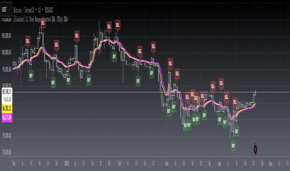
TASC 2022.09 LRAdj EMA█ OVERVIEW
TASC's September 2022 edition of Traders' Tips includes an article by Vitali Apirine titled "The Linear Regression-Adjusted Exponential Moving Average". This script implements the titular indicator presented in this article.
█ CONCEPT
The Linear Regression-Adjusted Exponential Moving Average (LRAdj EMA) is a new tool that combines a linear regression indicator with exponential moving averages . First, the indicator accounts for the linear regression deviation, that is, the distance between the price and the linear regression indicator. Subsequently, an exponential moving average (EMA) smooths the price data and and provides an indication of the current direction.
As part of a trading system, LRAdj EMA can be used in conjunction with an exponential moving average of the same length to identify the overall trend. Alternatively, using LRAdj EMAs of different lengths together can help identify turning points.
█ CALCULATION
The script uses the following input parameters:
EMA Length
LR Lookback Period
Multiplier
The calculation of LRAdj EMA is carried out as follows:
Current LRAdj EMA = Prior LRAdj EMA + MLTP × (1+ LRAdj × Multiplier ) × ( Price − Prior LRAdj EMA ),
where MLTP is a weighting multiplier defined as MLTP = 2 ⁄ ( EMA Length + 1), and LRAdj is the linear regression adjustment (LRAdj) multiplier:
LRAdj = (Abs( Current LR Dist )−Abs( Minimum LR Dist )) ⁄ (Abs( Maximum LR Dist )−Abs( Minimum LR Dist ))
When calculating the LRAdj multiplier, the absolute values of the following quantities are used:
Current LR Dist is the distance between the current close and the linear regression indicator with a length determined by the LR Lookback Period parameter,
Minimum LR Dist is the minimum distance between the close and the linear regression indicator for the LR lookback period ,
Maximum LR Dist is the maximum distance between the close and the linear regression indicator for the LR lookback period .
