Moving Averages ProxyLibrary "MovingAveragesProxy"
Moving Averages Proxy - Library of all moving averages spread out in different libraries
rvwap(_src, fixedTfInput, minsInput, hoursInput, daysInput, minBarsInput)
Calculates the Rolling VWAP (customized VWAP developed by the team of TradingView)
Parameters:
_src : (float) Source. Default: close
fixedTfInput : (bool) Use a fixed time period. Default: false
minsInput : (int) Minutes. Default: 0
hoursInput : (int) Hours. Default: 0
daysInput : (int) Days. Default: 1
minBarsInput : (int) Bars. Default: 10
Returns: (float) Rolling VWAP
correlationMa(src, len, factor)
Correlation Moving Average
Parameters:
src : (float) Source. Default: close
len : (int) Length
factor : (float) Factor. Default: 1.7
Returns: (float) Correlation Moving Average
regma(src, len, lambda)
Regularized Exponential Moving Average
Parameters:
src : (float) Source. Default: close
len : (int) Length
lambda : (float) Lambda. Default: 0.5
Returns: (float) Regularized Exponential Moving Average
repma(src, len)
Repulsion Moving Average
Parameters:
src : (float) Source. Default: close
len : (int) Length
Returns: (float) Repulsion Moving Average
epma(src, length, offset)
End Point Moving Average
Parameters:
src : (float) Source. Default: close
length : (int) Length
offset : (float) Offset. Default: 4
Returns: (float) End Point Moving Average
lc_lsma(src, length)
1LC-LSMA (1 line code lsma with 3 functions)
Parameters:
src : (float) Source. Default: close
length : (int) Length
Returns: (float) 1LC-LSMA Moving Average
aarma(src, length)
Adaptive Autonomous Recursive Moving Average
Parameters:
src : (float) Source. Default: close
length : (int) Length
Returns: (float) Adaptive Autonomous Recursive Moving Average
alsma(src, length)
Adaptive Least Squares
Parameters:
src : (float) Source. Default: close
length : (int) Length
Returns: (float) Adaptive Least Squares
ahma(src, length)
Ahrens Moving Average
Parameters:
src : (float) Source. Default: close
length : (int) Length
Returns: (float) Ahrens Moving Average
adema(src)
Ahrens Moving Average
Parameters:
src : (float) Source. Default: close
Returns: (float) Moving Average
autol(src, lenDev)
Auto-Line
Parameters:
src : (float) Source. Default: close
lenDev : (int) Length for standard deviation
Returns: (float) Auto-Line
fibowma(src, length)
Fibonacci Weighted Moving Average
Parameters:
src : (float) Source. Default: close
length : (int) Length
Returns: (float) Moving Average
fisherlsma(src, length)
Fisher Least Squares Moving Average
Parameters:
src : (float) Source. Default: close
length : (int) Length
Returns: (float) Moving Average
leoma(src, length)
Leo Moving Average
Parameters:
src : (float) Source. Default: close
length : (int) Length
Returns: (float) Moving Average
linwma(src, period, weight)
Linear Weighted Moving Average
Parameters:
src : (float) Source. Default: close
period : (int) Length
weight : (int) Weight
Returns: (float) Moving Average
mcma(src, length)
McNicholl Moving Average
Parameters:
src : (float) Source. Default: close
length : (int) Length
Returns: (float) Moving Average
srwma(src, length)
Square Root Weighted Moving Average
Parameters:
src : (float) Source. Default: close
length : (int) Length
Returns: (float) Moving Average
EDSMA(src, len)
Ehlers Dynamic Smoothed Moving Average.
Parameters:
src : Series to use ('close' is used if no argument is supplied).
len : Lookback length to use.
Returns: EDSMA smoothing.
dema(x, t)
Double Exponential Moving Average.
Parameters:
x : Series to use ('close' is used if no argument is supplied).
t : Lookback length to use.
Returns: DEMA smoothing.
tema(src, len)
Triple Exponential Moving Average.
Parameters:
src : Series to use ('close' is used if no argument is supplied).
len : Lookback length to use.
Returns: TEMA smoothing.
smma(src, len)
Smoothed Moving Average.
Parameters:
src : Series to use ('close' is used if no argument is supplied).
len : Lookback length to use.
Returns: SMMA smoothing.
hullma(src, len)
Hull Moving Average.
Parameters:
src : Series to use ('close' is used if no argument is supplied).
len : Lookback length to use.
Returns: Hull smoothing.
frama(x, t)
Fractal Reactive Moving Average.
Parameters:
x : Series to use ('close' is used if no argument is supplied).
t : Lookback length to use.
Returns: FRAMA smoothing.
kama(x, t)
Kaufman's Adaptive Moving Average.
Parameters:
x : Series to use ('close' is used if no argument is supplied).
t : Lookback length to use.
Returns: KAMA smoothing.
vama(src, len)
Volatility Adjusted Moving Average.
Parameters:
src : Series to use ('close' is used if no argument is supplied).
len : Lookback length to use.
Returns: VAMA smoothing.
donchian(len)
Donchian Calculation.
Parameters:
len : Lookback length to use.
Returns: Average of the highest price and the lowest price for the specified look-back period.
Jurik(src, len)
Jurik Moving Average.
Parameters:
src : Series to use ('close' is used if no argument is supplied).
len : Lookback length to use.
Returns: JMA smoothing.
xema(src, len)
Optimized Exponential Moving Average.
Parameters:
src : Series to use ('close' is used if no argument is supplied).
len : Lookback length to use.
Returns: XEMA smoothing.
ehma(src, len)
EHMA - Exponential Hull Moving Average
Parameters:
src : Source
len : Period
Returns: Exponential Hull Moving Average (EHMA)
covwema(src, len)
Coefficient of Variation Weighted Exponential Moving Average (COVWEMA)
Parameters:
src : Source
len : Period
Returns: Coefficient of Variation Weighted Exponential Moving Average (COVWEMA)
covwma(src, len)
Coefficient of Variation Weighted Moving Average (COVWMA)
Parameters:
src : Source
len : Period
Returns: Coefficient of Variation Weighted Moving Average (COVWMA)
eframa(src, len, FC, SC)
Ehlrs Modified Fractal Adaptive Moving Average (EFRAMA)
Parameters:
src : Source
len : Period
FC : Lower Shift Limit for Ehlrs Modified Fractal Adaptive Moving Average
SC : Upper Shift Limit for Ehlrs Modified Fractal Adaptive Moving Average
Returns: Ehlrs Modified Fractal Adaptive Moving Average (EFRAMA)
etma(src, len)
Exponential Triangular Moving Average (ETMA)
Parameters:
src : Source
len : Period
Returns: Exponential Triangular Moving Average (ETMA)
rma(src, len)
RMA - RSI Moving average
Parameters:
src : Source
len : Period
Returns: RSI Moving average (RMA)
thma(src, len)
THMA - Triple Hull Moving Average
Parameters:
src : Source
len : Period
Returns: Triple Hull Moving Average (THMA)
vidya(src, len)
Variable Index Dynamic Average (VIDYA)
Parameters:
src : Source
len : Period
Returns: Variable Index Dynamic Average (VIDYA)
zsma(src, len)
Zero-Lag Simple Moving Average (ZSMA)
Parameters:
src : Source
len : Period
Returns: Zero-Lag Simple Moving Average (ZSMA)
zema(src, len)
Zero-Lag Exponential Moving Average (ZEMA)
Parameters:
src : Source
len : Period
Returns: Zero-Lag Exponential Moving Average (ZEMA)
evwma(src, len)
EVWMA - Elastic Volume Weighted Moving Average
Parameters:
src : Source
len : Period
Returns: Elastic Volume Weighted Moving Average (EVWMA)
tt3(src, len, a1_t3)
Tillson T3
Parameters:
src : Source
len : Period
a1_t3 : Tillson T3 Volume Factor
Returns: Tillson T3
gma(src, len)
GMA - Geometric Moving Average
Parameters:
src : Source
len : Period
Returns: Geometric Moving Average (GMA)
wwma(src, len)
WWMA - Welles Wilder Moving Average
Parameters:
src : Source
len : Period
Returns: Welles Wilder Moving Average (WWMA)
cma(src, len)
Corrective Moving average (CMA)
Parameters:
src : Source
len : Period
Returns: Corrective Moving average (CMA)
edma(src, len)
Exponentially Deviating Moving Average (MZ EDMA)
Parameters:
src : Source
len : Period
Returns: Exponentially Deviating Moving Average (MZ EDMA)
rema(src, len)
Range EMA (REMA)
Parameters:
src : Source
len : Period
Returns: Range EMA (REMA)
sw_ma(src, len)
Sine-Weighted Moving Average (SW-MA)
Parameters:
src : Source
len : Period
Returns: Sine-Weighted Moving Average (SW-MA)
mama(src, len)
MAMA - MESA Adaptive Moving Average
Parameters:
src : Source
len : Period
Returns: MESA Adaptive Moving Average (MAMA)
fama(src, len)
FAMA - Following Adaptive Moving Average
Parameters:
src : Source
len : Period
Returns: Following Adaptive Moving Average (FAMA)
hkama(src, len)
HKAMA - Hilbert based Kaufman's Adaptive Moving Average
Parameters:
src : Source
len : Period
Returns: Hilbert based Kaufman's Adaptive Moving Average (HKAMA)
getMovingAverage(type, src, len, lsmaOffset, inputAlmaOffset, inputAlmaSigma, FC, SC, a1_t3, fixedTfInput, daysInput, hoursInput, minsInput, minBarsInput, lambda, volumeWeighted, gamma_aarma, smooth, linweight, volatility_lookback, jurik_phase, jurik_power)
Abstract proxy function that invokes the calculation of a moving average according to type
Parameters:
type : (string) Type of moving average
src : (float) Source of series (close, high, low, etc.)
len : (int) Period of loopback to calculate the average
lsmaOffset : (int) Offset for Least Squares MA
inputAlmaOffset : (float) Offset for ALMA
inputAlmaSigma : (float) Sigma for ALMA
FC : (int) Lower Shift Limit for Ehlrs Modified Fractal Adaptive Moving Average
SC : (int) Upper Shift Limit for Ehlrs Modified Fractal Adaptive Moving Average
a1_t3 : (float) Tillson T3 Volume Factor
fixedTfInput : (bool) Use a fixed time period in Rolling VWAP
daysInput : (int) Days in Rolling VWAP
hoursInput : (int) Hours in Rolling VWAP
minsInput : (int) Minutrs in Rolling VWAP
minBarsInput : (int) Bars in Rolling VWAP
lambda : (float) Regularization Constant in Regularized EMA
volumeWeighted : (bool) Apply volume weighted calculation in selected moving average
gamma_aarma : (float) Gamma for Adaptive Autonomous Recursive Moving Average
smooth : (float) Smooth for Adaptive Least Squares
linweight : (float) Weight for Volume Weighted Moving Average
volatility_lookback : (int) Loopback for Volatility Adjusted Moving Average
jurik_phase : (int) Phase for Jurik Moving Average
jurik_power : (int) Power for Jurik Moving Average
Returns: (float) Moving average
Cerca negli script per "Fractal"
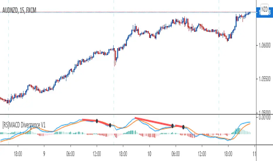
[RS]MACD Divergence V1This oscilator was created by Ricardo Santos using MACD's histogram as the series to find low and high fractals and from there find and plot divergences.
I just modified it a little bit to make it to look more like the MACD public library indicator and use the actual MACD series (instead of the histogram) to find the fractals and from there plot divergences.
I did this to make it easier for me and other fellow students of a Forex school where we use these type of divergences to find patterns.
Ichimoku ++ public v0.9Description:
The intention of this script is to build/provide a kind of work station / work bench for analysing markets and especially Bitcoin . Another goal is to get maximum market information while maintaining a good chart overview. A chart overloaded with indicators is useless because it obscures the view of the chart as the most important indicator. The chart should be clear and market structure should be easy to see. In addition, some indicator signals can be activated to better assess the quality of signals from the past. The chart environment or the chart context is important for the quality of a signal.
The intention of this script is not to teach someone how to trade or how to use these Indicators but to provide a tool to analyse markets better and to help to draw conclusions of market behaviour in a higher quality.
A general advise:
Use the included indicators and signals in a confluent way to get stoploss, buy and sell entry points. SR clusters can be identified for use in conjunction with fractals as entry and exit pints. My other scripts can also help. Prefer 4 hours, daily and a longer time frame. There is no "Holy Grail" :).
If someone is new to trading you should learn about the indicators first. Definitely learn about Ichimoku Cloud Indicator.
Integrated indicators are:
Ichimoku Cloud and signals
Parabolic SAR and signal
ATR stop
Bollinger Bands
EMA / SMA and background color as signal
Williams Fractals and signal
Puell Multiple signal

Trend-Following Combo-SuperTrend, EMA, Aroon, DMI, Laguerre RSIThis is a trend-following indicator which condenses two SuperTrend indicators -- one based on analysis over a shorter period of time (1.5, 7), and one based on analysis over a longer period of time (1.65, 100) -- into a single indicator which appears on your chart only when both the shorter- and longer-term analysis indicates a "SuperTrend" in the same direction.
Additionally, potential trade entry indicators are displayed in the form of up and down arrows when (by default) three of the following five indicators suggest that the market is trending in the same direction as both the shorter- and longer-term SuperTrend indicators:
EMA Crossover (8, 15)
Aroon Indicator (8)
Aroon Oscillator (8)
Directional Movement Index (DI +/-) (8)
Laguerre RSI (13)
You may update the parameters of any of the indicators to match your own preferences.
Additionally, you may also adjust the "Threshold" of indicators that must be in agreement with the SuperTrend to show a potential trade entry arrow. Bear in mind that if you set the Indicator Threshold too low, you will see more frequent trade entry arrows, many of which will not be profitable if taken. Similarly, set this value too high, and you will see fewer trade entry arrows that may not appear until after most of the "juice" in the trend has evaporated. Ideal values for the threshold seem to be between 2-4, depending on the symbol you are trading.
The following image shows all of the indicators referenced above on a 5-minute chart of the SPY during a single trading day:
And, here is the same period of time showing only the Trend-Following Combo indicator with default settings:
This indicator would not have been possible save for work contributed by the following:
SuperTrend by Rajandran R
Aroon w/ crossovers highlighted by seiglerj
Aroon Oscillator by jcrewolinsky
Directional Movement Index by TradingView
Laguerre RSI (Self Adjusting Alpha with Fractals Energy) by everget

Uncle Mo's Ultimate Ichimoku V1Main features:
2 x Ichimoku Cloud
5 x EMA
2 x MA
1 x HullMA
Williams Fractals
Study is based around trader @br0qn 's Ichimoku script.
Credits also go to:
@RicardoSantos for the Bill Williams Fractals
@EmilianoMesa for the EMAs/MAs
@mohamed982 for the HullMA
The script is open source so please feel free to change it around. I'd greatly appreciate it if you could suggest ways to improve it.
Happy trading!

Iridescent Liquidity Prism [JOAT]Iridescent Liquidity Prism | Peer Momentum HUD
A multi-layered order-flow indicator that combines microstructure analysis, smart-money footprint detection, and intermarket momentum signals. The script uses dynamic color-shifting themes to visualize liquidity patterns, structure, and peer momentum data directly on the chart.
There is so much to choose from inside the settings, if you think it's a mess on the chart it's because you have to personally customize it based on your needs...
Core Functionality
The indicator calculates and displays several analytical layers simultaneously:
Order-Flow Imbalance (OFI): Calculates buy vs. sell volume pressure using volume-weighted price distribution within each bar. Uses an EMA filter (default: 55 periods) to smooth the signal. Values are normalized using standard deviation to identify significant imbalances.
Smart Money Footprints: Detects accumulation and distribution zones by comparing volume rate of change (ROC) against price ROC. When volume ROC exceeds a threshold (default: 65%) and price ROC is positive, accumulation is detected. When volume ROC is high but price ROC is negative, distribution is detected.
Fractal Structure Mapping: Identifies pivot highs and lows using a fractal detection algorithm (default: 5-bar period). Maintains a rolling window of recent structure points (default: 4 levels) and draws connecting lines to show trend structure.
Fair Value Gap (FVG) Detection: Automatically detects price gaps where three consecutive candles create an imbalance. Bullish FVGs occur when the current low exceeds the high two bars ago. Bearish FVGs occur when the current high is below the low two bars ago. Gaps persist for a configurable duration (default: 320 bars) and fade when price fills the gap.
Liquidity Void Detection: Identifies candles where the high-low range exceeds an ATR threshold (default: 1.7x ATR) while volume is below average (default: 65% of 20-bar average). These conditions suggest areas where liquidity may be thin.
Price/Volume Divergence: Uses linear regression to detect when price trend direction disagrees with volume trend direction. A divergence alert appears when price is trending up while volume is trending down, or vice versa.
Peer Momentum Heatmap (PMH): Calculates composite momentum scores for up to 6 symbols across 4 timeframes. Each score combines RSI (default: 14 periods) and StochRSI (default: 14 periods, 3-bar smooth) to create a momentum composite between -1 and +1. The highest absolute momentum score across all combinations is displayed in the HUD.
Custom settings using Fractal Pivots, Skeleton Structure, Pulse Liquidity Voids, Bottom Colorful HeatMaps, and Iridescent Field.
---
Visual Components
Spectrum Aura Glow: ATR-weighted bands (default: 0.25x ATR) that expand and contract around price action, indicating volatility conditions. The thickness adapts to market volatility.
Chromatic Flow Trail: A blended line combining EMA and WMA of price (default: 8-period EMA blended with WMA at 65% ratio). The trail uses gradient colors that shift based on a phase oscillator, creating an iridescent effect.
Volume Heat Projection: Creates horizontal volume profile bands at price levels (default: 14 levels). Scans recent bars (default: 150 bars) to calculate volume concentration. Each level is colored based on its volume density relative to the maximum volume level.
Structure Skeleton: Dashed lines connecting fractal pivot points. Uses two layers: a primary line (2-3px width) and an optional glow overlay (4-5px width) for enhanced visibility.
Fractal Markers: Diamond shapes placed at pivot high and low points. Color-coded: primary color for highs, secondary color for lows.
Iridescent Color Themes: Five color themes available: Iridescent (default), Pearlescent, Prismatic, ColorShift, and Metallic. Colors shift dynamically using a phase oscillator that cycles through the color spectrum based on bar index and a speed multiplier (default: 0.35).
---
HUD Console Metrics
The right-side HUD displays seven key metrics:
Flow: Shows OFI status: ▲ FLOW BUY when normalized OFI exceeds imbalance threshold (default: 2.2), ▼ FLOW SELL when below -2.2, or ◆ FLOW BAL when balanced.
Struct: Structure trend bias: ▲ STRUCT BULL when microtrend > 2, ▼ STRUCT BEAR when < -2, or ◆ STRUCT RANGE when neutral.
Smart$: Institutional activity: ◈ ACCUM when smart money index = 1, ◈ DISTRIB when = -1, or ○ IDLE when inactive.
Liquid: Liquidity state: ⚡ VOID when a liquidity void is detected, or ● NORMAL otherwise.
Diverg: Divergence status: ⚠ ALERT when price/volume divergence detected, or ✓ CLEAR when aligned.
PMH: Peer Momentum Heatmap status: Shows dominant timeframe and momentum score. Displays 🪩 for bull surge (above 0.55 threshold) or 🧨 for bear surge (below -0.55).
FVG: Fair Value Gap status: Shows active gap count or CLEAR when no gaps exist. Displays GAP LONG when bullish gap detected, GAP SHORT when bearish gap detected.
Pearlscent Color with Volume Heatmap.
Parameters and Settings
Microstructure Engine:
Analysis Depth: 20-250 bars (default: 55) - Controls OFI smoothing period
Liquidity Threshold ATR: 1.0-4.0 (default: 1.7) - Multiplier for void detection
Imbalance Ratio: 1.5-6.0 (default: 2.2) - Standard deviations for OFI significance
Smart Money Layer:
Smart Money Window: 10-150 bars (default: 24) - Period for ROC calculations
Accumulation Threshold: 40-95% (default: 65%) - Volume ROC threshold
Structural Mapping:
Fractal Pivot Period: 3-15 bars (default: 5) - Period for pivot detection
Structure Memory: 2-8 levels (default: 4) - Number of structure points to track
Volume Heat Projection:
Heat Map Lookback: 60-400 bars (default: 150) - Bars to analyze for volume profile
Heat Map Levels: 5-30 levels (default: 14) - Number of price level bands
Heat Map Opacity: 40-100% (default: 92%) - Transparency of heat map boxes
Heat Map Width Limit: 6-80 bars (default: 26) - Maximum width of heat map boxes
Heat Map Visibility Threshold: 0.0-0.5 (default: 0.08) - Minimum density to display
Iridescent Enhancements:
Visual Theme: Iridescent, Pearlescent, Prismatic, ColorShift, or Metallic
Color Shift Speed: 0.05-1.00 (default: 0.35) - Speed of color phase oscillation
Aura Thickness (ATR): 0.05-1.0 (default: 0.25) - Multiplier for aura band width
Chromatic Trail Length: 2-50 bars (default: 8) - Period for trail calculation
Trail Blend Ratio: 0.1-0.95 (default: 0.65) - EMA/WMA blend percentage
FVG Persistence: 50-600 bars (default: 320) - Bars to keep FVG boxes active
Max Active FVG Boxes: 10-200 (default: 40) - Maximum boxes on chart
FVG Base Opacity: 20-95% (default: 80%) - Transparency of FVG boxes
Peer Momentum Heatmap:
Peer Symbols: Comma-separated list of up to 6 symbols (e.g., "BTCUSD,ETHUSD")
Peer Timeframes: Comma-separated list of up to 4 timeframes (default: "60,240,D")
PMH RSI Length: 5-50 periods (default: 14)
PMH StochRSI Length: 5-50 periods (default: 14)
PMH StochRSI Smooth: 1-10 periods (default: 3)
Super Momentum Threshold: 0.2-0.95 (default: 0.55) - Threshold for surge detection
Clarity & Readability:
Liquidity Void Opacity: 5-90% (default: 30%)
Smart Money Footprint Opacity: 5-90% (default: 35%)
HUD Background Opacity: 40-95% (default: 70%)
Iridescent Field:
Field Opacity: 20-100% (default: 86%) - Background color intensity
Field Smooth Length: 10-200 bars (default: 34) - Smoothing for background gradient
---
Alerts
The indicator provides seven alert conditions:
Liquidity Void Detected - Triggers when void conditions are met
Strong Order Flow - Triggers when normalized OFI exceeds imbalance ratio
Smart Money Activity - Triggers when accumulation or distribution detected
Price/Volume Divergence - Triggers when divergence conditions occur
Structure Shift - Triggers when structure polarity changes significantly
PMH Bull Surge - Triggers when PMH exceeds positive threshold (if enabled)
PMH Bear Surge - Triggers when PMH exceeds negative threshold (if enabled)
Bull/Bear Prismatic FVG - Triggers when new FVG is detected (if FVG display enabled)
---
Usage Considerations
Performance may vary on lower timeframes due to the volume heat map calculations scanning multiple bars. Consider reducing heat map lookback or levels if experiencing slowdowns.
The PMH feature requires data requests to other symbols/timeframes, which may impact performance. Limit the number of peer symbols and timeframes for optimal performance.
FVG boxes automatically expire after the persistence period to prevent chart clutter. The maximum box limit (default: 40) prevents excessive memory usage.
Color themes affect all visual elements. Choose a theme that provides good contrast with your chart background.
The indicator is designed for overlay display. All visual elements are positioned relative to price action.
Structure lines are drawn dynamically as new pivots form. On fast-moving markets, structure may update frequently.
Volume calculations assume typical volume data availability. Symbols without volume may show incomplete data for volume-dependent features.
---
Technical Notes
Built on Pine Script v6 with dynamic request capability for PMH functionality.
Uses exponential moving averages (EMA) and weighted moving averages (WMA) for trail calculations to balance responsiveness and smoothness.
Volume profile calculation uses price level buckets. Higher levels provide finer granularity but require more computation.
Iridescent color engine uses a phase oscillator with sine wave calculations for smooth color transitions.
Box management includes automatic cleanup of expired boxes to maintain performance.
All visual elements use color gradients and transparency for smooth blending with price action.
---
Customization Examples
Intraday Scalping Setup:
Analysis Depth: 30 bars
Heat Map Lookback: 100 bars
FVG Persistence: 150 bars
PMH Window: 15 bars
Fast color shift speed: 0.5+
Macro Structure Tracking:
Analysis Depth: 100+ bars
Heat Map Lookback: 300+ bars
FVG Persistence: 500+ bars
Structure Memory: 6-8 levels
Slower color shift speed: 0.2
---
Limitations
Volume heat map calculations may be computationally intensive on lower timeframes with high lookback values.
PMH requires valid symbol names and accessible timeframes. Invalid symbols or timeframes will return no data.
FVG detection requires at least 3 bars of history. Early bars may not show FVG boxes.
Structure lines connect points but do not predict future structure. They reflect historical pivot relationships.
Color themes are aesthetic choices and do not affect calculation logic.
The indicator does not provide trading signals. All visual elements are analytical tools that require interpretation in context of market conditions.
Open Source
This indicator is open source and available for modification and distribution. The code is published with Pine Script v6 compliance. Users are free to customize parameters, modify calculations, and adapt the visual elements to their trading needs.
For questions, suggestions, or anything please talk to me in private messages or comments below!
Would love to help!
- officialjackofalltrades

LETHINH-Swing pa,smc🟦 📌 Title (English)
Swing High / Swing Low – 3-Candle Fractal (5-Bar Pivot) | Auto Alerts
⸻
🟩 📌 Short Description
A clean and reliable swing high / swing low detector based on the classic 3-candle (5-bar) fractal pivot. Automatically marks SH/SL and triggers alerts when a swing is confirmed. No repainting after confirmation.
⸻
🟧 📌 Full Description (for TradingView Publishing)
🔶 Swing High / Swing Low – 3-Candle Fractal (5-Bar Pivot)
This indicator identifies Swing Highs (SH) and Swing Lows (SL) using the classic 3-candle fractal pattern, also known as the 5-bar pivot.
It marks swing points only after full confirmation, making it highly reliable and suitable for structure-based trading.
⸻
🔶 📍 How It Works
A swing is confirmed when the center candle is higher (or lower) than the two candles on each side:
Swing High (SH)
high > high , high , high
Swing Low (SL)
low < low , low , low
The confirmation occurs after 2 right candles close, so the indicator does not repaint once a swing is identified.
⸻
🔶 📍 Key Features
• Detects clean and accurate swings
• Uses pure price action — no indicators, no lag
• Marks swing high (SH) and swing low (SL) directly on the chart
• Non-repainting after confirmation
• Works on all timeframes and all markets
• Extremely lightweight and fast
• Includes alert conditions for both SH and SL
Perfect for traders using:
• Market Structure (BOS / CHoCH)
• Order Blocks (OB)
• Smart Money Concepts (SMC)
• Liquidity hunts
• Wyckoff
• Support/Resistance
• Price Action entries
⸻
🔶 📍 Why This Indicator Is Useful
Swing points are the foundation of market structure.
Accurately detecting them helps traders:
• Identify trend shifts
• Spot BOS / CHoCH correctly
• Find key zones (OB, liquidity levels, supply/demand)
• Time entries more precisely
• Avoid fake structure breaks
This indicator ensures swings are plotted only when fully confirmed, reducing noise and confusion.
⸻
🔶 📍 Alerts
You can create alerts for both conditions:
• Swing High Confirmed
• Swing Low Confirmed
Recommended settings:
• Once per bar close
• Open-ended alert
With alerts enabled, TradingView will automatically notify you every time a new swing forms.
⸻
🔶 📍 No Repainting
Once a swing is confirmed and plotted, it will not change or disappear.
This makes the indicator reliable for real-time alerts and backtesting.
⸻
🔶 📍 Pine Script (v5)
Paste your indicator code here if you want it visible.
Or leave the code hidden if you are publishing as protected.
⸻
🔶 📍 Final Notes
• This indicator focuses on confirmation, not prediction
• It is designed for clean structure reading
• All markets supported: Forex, Crypto, Stocks, Indexes, Commodities
• Suitable for scalping, intraday, swing, and even higher-timeframe trading
If you find this tool helpful, feel free to give it a like and add it to your favorites ❤️
Your support helps me share more tools with the community!

TAUtilityLibLibrary "TAUtilityLib"
Technical Analysis Utility Library - Collection of functions for market analysis, smoothing, scaling, and structure detection
log_snapshot(label1, val1, label2, val2, label3, val3, label4, val4, label5, val5)
Creates formatted log snapshot with 5 labeled values
Parameters:
label1 (string)
val1 (float)
label2 (string)
val2 (float)
label3 (string)
val3 (float)
label4 (string)
val4 (float)
label5 (string)
val5 (float)
Returns: void (logs to console)
f_get_next_tf(tf, steps)
Gets next higher timeframe(s) from current
Parameters:
tf (string) : Current timeframe string
steps (string) : "1 TF Higher" for next TF, any other value for 2 TFs higher
Returns: Next timeframe string or na if at maximum
f_get_prev_tf(tf)
Gets previous lower timeframe from current
Parameters:
tf (string) : Current timeframe string
Returns: Previous timeframe string or na if at minimum
supersmoother(_src, _length)
Ehler's SuperSmoother - low-lag smoothing filter
Parameters:
_src (float) : Source series to smooth
_length (simple int) : Smoothing period
Returns: Smoothed series
butter_smooth(src, len)
Butterworth filter for ultra-smooth price filtering
Parameters:
src (float) : Source series
len (simple int) : Filter period
Returns: Butterworth smoothed series
f_dynamic_ema(source, dynamic_length)
Dynamic EMA with variable length
Parameters:
source (float) : Source series
dynamic_length (float) : Dynamic period (can vary bar to bar)
Returns: Dynamically adjusted EMA
dema(source, length)
Double Exponential Moving Average (DEMA)
Parameters:
source (float) : Source series
length (simple int) : Period for DEMA calculation
Returns: DEMA value
f_scale_percentile(primary_line, secondary_line, x)
Scales secondary line to match primary line using percentile ranges
Parameters:
primary_line (float) : Reference series for target scale
secondary_line (float) : Series to be scaled
x (int) : Lookback bars for percentile calculation
Returns: Scaled version of secondary_line
calculate_correlation_scaling(demamom_range, demamom_min, correlation_range, correlation_min)
Calculates scaling factors for correlation alignment
Parameters:
demamom_range (float) : Range of primary series
demamom_min (float) : Minimum of primary series
correlation_range (float) : Range of secondary series
correlation_min (float) : Minimum of secondary series
Returns: tuple for alignment
getBB(src, length, mult, chartlevel)
Calculates Bollinger Bands with chart level offset
Parameters:
src (float) : Source series
length (simple int) : MA period
mult (simple float) : Standard deviation multiplier
chartlevel (simple float) : Vertical offset for plotting
Returns: tuple
get_mrc(source, length, mult, mult2, gradsize)
Mean Reversion Channel with multiple bands and conditions
Parameters:
source (float) : Price source
length (simple int) : Channel period
mult (simple float) : First band multiplier
mult2 (simple float) : Second band multiplier
gradsize (simple float) : Gradient size for zone detection
Returns:
analyzeMarketStructure(highFractalBars, highFractalPrices, lowFractalBars, lowFractalPrices, trendDirection)
Analyzes market structure for ChoCH and BOS patterns
Parameters:
highFractalBars (array) : Array of high fractal bar indices
highFractalPrices (array) : Array of high fractal prices
lowFractalBars (array) : Array of low fractal bar indices
lowFractalPrices (array) : Array of low fractal prices
trendDirection (int) : Current trend (1=up, -1=down, 0=neutral)
Returns: - change signals and new trend direction

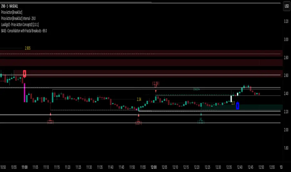
Price Action [BreakOut] InternalKey Features and Functionality
Support & Resistance (S/R): The script automatically identifies and draws support and resistance lines based on a user-defined "swing period." These lines are drawn from recent pivot points, and users can customize their appearance, including color, line style (solid, dashed, dotted), and extension (left, right, or both). The indicator can also display the exact price of each S/R level.
Trendlines: It draws trendlines connecting pivot highs and pivot lows. This feature helps visualize the current trend direction. Users can choose to show only the newest trendlines, customize their length and style, and select the source for the pivot points (e.g., candle close or high/low shadow).
Price Action Pivots: This is a core component that identifies and labels different types of pivots based on price action: Higher Highs (HH), Lower Highs (LH), Higher Lows (HL), and Lower Lows (LL). These pivots are crucial for understanding market structure and identifying potential trend changes. The script marks these pivots with shapes and can display their price values.
Fractal Breakouts: The script identifies and signals "fractal breakouts" and "breakdowns" when the price closes above a recent high pivot or below a recent low pivot, respectively. These signals are visually represented with up (⬆) and down (⬇) arrow symbols on the chart.
Customization and Alerts: The indicator is highly customizable. You can toggle on/off various features (S/R, trendlines, pivots, etc.), adjust colors, line styles, and text sizes. It also includes an extensive list of alert conditions, allowing traders to receive notifications for:
Price Crossovers: When the close price crosses over or under a support or resistance level.
Trendline Breaks: When the price breaks above an upper trendline or below a lower trendline.
Fractal Breaks: When a fractal breakout or breakdown occurs.
Information-Geometric Market DynamicsInformation-Geometric Market Dynamics
The Information Field: A Geometric Approach to Market Dynamics
By: DskyzInvestments
Foreword: Beyond the Shadows on the Wall
If you have traded for any length of time, you know " the feeling ." It is the frustration of a perfect setup that fails, the whipsaw that stops you out just before the real move, the nagging sense that the chart is telling you only half the story. For decades, technical analysis has relied on interpreting the shadows—the patterns left behind by price. We draw lines on these shadows, apply indicators to them, and hope they reveal the future.
But what if we could stop looking at the shadows and, instead, analyze the object casting them?
This script introduces a new paradigm for market analysis: Information-Geometric Market Dynamics (IGMD) . The core premise of IGMD is that the price chart is merely a one-dimensional projection of a much richer, higher-dimensional reality—an " information field " generated by the collective actions and beliefs of all market participants.
This is not just another collection of indicators. It is a unified framework for measuring the geometry of the market's information field—its memory, its complexity, its uncertainty, its causal flows—and making high-probability decisions based on that deeper reality. By fusing advanced mathematical and informational concepts, IGMD provides a multi-faceted lens through which to view market behavior, moving beyond simple price action into the very structure of market information itself.
Prepare to move beyond the flatland of the price chart. Welcome to the information field.
The IGMD Framework: A Multi-Kernel Approach
What is a Kernel? The Heart of Transformation
In mathematics and data science, a kernel is a powerful and elegant concept. At its core, a kernel is a function that takes complex, often inscrutable data and transforms it into a more useful format. Think of it as a specialized lens or a mathematical "probe." You cannot directly measure abstract concepts like "market memory" or "trend quality" by looking at a price number. First, you must process the raw price data through a specific mathematical machine—a kernel—that is designed to output a measurement of that specific property. Kernels operate by performing a sort of "similarity test," projecting data into a higher-dimensional space where hidden patterns and relationships become visible and measurable.
Why do creators use them? We use kernels to extract features —meaningful pieces of information—that are not explicitly present in the raw data. They are the essential tools for moving beyond surface-level analysis into the very DNA of market behavior. A simple moving average can tell you the average price; a suite of well-chosen kernels can tell you about the character of the price action itself.
The Alchemist's Challenge: The Art of Fusion
Using a single kernel is a challenge. Using five distinct, computationally demanding mathematical engines in unison is an immense undertaking. The true difficulty—and artistry—lies not just in using one kernel, but in fusing the outputs of many . Each kernel provides a different perspective, and they can often give conflicting signals. One kernel might detect a strong trend, while another signals rising chaos and uncertainty. The IGMD script's greatest strength is its ability to act as this alchemist, synthesizing these disparate viewpoints through a weighted fusion process to produce a single, coherent picture of the market's state. It required countless hours of testing and calibration to balance the influence of these five distinct analytical engines so they work in harmony rather than cacophony.
The Five Kernels of Market Dynamics
The IGMD script is built upon a foundation of five distinct kernels, each chosen to probe a unique and critical dimension of the market's information field.
1. The Wavelet Kernel (The "Microscope")
What it is: The Wavelet Kernel is a signal processing function designed to decompose a signal into different frequency scales. Unlike a Fourier Transform that analyzes the entire signal at once, the wavelet slides across the data, providing information about both what frequencies are present and when they occurred.
The Kernels I Use:
Haar Kernel: The simplest wavelet, a square-wave shape defined by the coefficients . It excels at detecting sharp, sudden changes.
Daubechies 2 (db2) Kernel: A more complex and smoother wavelet shape that provides a better balance for analyzing the nuanced ebb and flow of typical market trends.
How it Works in the Script: This kernel is applied iteratively. It first separates the finest "noise" (detail d1) from the first level of trend (approximation a1). It then takes the trend a1 and repeats the process, extracting the next level of cycle (d2) and trend (a2), and so on. This hierarchical decomposition allows us to separate short-term noise from the long-term market "thesis."
2. The Hurst Exponent Kernel (The "Memory Gauge")
What it is: The Hurst Exponent is derived from a statistical analysis kernel that measures the "long-term memory" or persistence of a time series. It is the definitive measure of whether a series is trending (H > 0.5), mean-reverting (H < 0.5), or random (H = 0.5).
How it Works in the Script: The script employs a method based on Rescaled Range (R/S) analysis. It calculates the average range of price movements over increasingly larger time lags (m1, m2, m4, m8...). The slope of the line plotting log(range) vs. log(lag) is the Hurst Exponent. Applying this complex statistical analysis not to the raw price, but to the clean, wavelet-decomposed trend lines, is a key innovation of IGMD.
3. The Fractal Dimension Kernel (The "Complexity Compass")
What it is: This kernel measures the geometric complexity or "jaggedness" of a price path, based on the principles of fractal geometry. A straight line has a dimension of 1; a chaotic, space-filling line approaches a dimension of 2.
How it Works in the Script: We use a version based on Ehlers' Fractal Dimension Index (FDI). It calculates the rate of price change over a full lookback period (N3) and compares it to the sum of the rates of change over the two halves of that period (N1 + N2). The formula d = (log(N1 + N2) - log(N3)) / log(2) quantifies how much "longer" and more convoluted the price path was than a simple straight line. This kernel is our primary filter for tradeable (low complexity) vs. untradeable (high complexity) conditions.
4. The Shannon Entropy Kernel (The "Uncertainty Meter")
What it is: This kernel comes from Information Theory and provides the purest mathematical measure of information, surprise, or uncertainty within a system. It is not a measure of volatility; a market moving predictably up by 10 points every bar has high volatility but zero entropy .
How it Works in the Script: The script normalizes price returns by the ATR, categorizes them into a discrete number of "bins" over a lookback window, and forms a probability distribution. The Shannon Entropy H = -Σ(p_i * log(p_i)) is calculated from this distribution. A low H means returns are predictable. A high H means returns are chaotic. This kernel is our ultimate gauge of market conviction.
5. The Transfer Entropy Kernel (The "Causality Probe")
What it is: This is by far the most advanced and computationally intensive kernel in the script. Transfer Entropy is a non-parametric measure of directed information flow between two time series. It moves beyond correlation to ask: "Does knowing the past of Volume genuinely reduce our uncertainty about the future of Price?"
How it Works in the Script: To make this work, the script discretizes both price returns and the chosen "driver" (e.g., OBV) into three states: "up," "down," or "neutral." It then builds complex conditional probability tables to measure the flow of information in both directions. The Net Transfer Entropy (TE Driver→Price minus TE Price→Driver) gives us a direct measure of causality . A positive score means the driver is leading price, confirming the validity of the move. This is a profound leap beyond traditional indicator analysis.
Chapter 3: Fusion & Interpretation - The Field Score & Dashboard
Each kernel is a specialist providing a piece of the puzzle. The Field Score is where they are fused into a single, comprehensive reading. It's a weighted sum of the normalized scores from all five kernels, producing a single number from -1 (maximum bearish information field) to +1 (maximum bullish information field). This is the ultimate "at-a-glance" metric for the market's net state, and it is interpreted through the dashboard.
The Dashboard: Your Mission Control
Field Score & Regime: The master metric and its plain-English interpretation ("Uptrend Field", "Downtrend Field", "Transitional").
Kernel Readouts (Wave Align, H(w), FDI, etc.): The live scores of each individual kernel. This allows you to see why the Field Score is what it is. A high Field Score with all components in agreement (all green or red) is a state of High Coherence and represents a high-quality setup.
Market Context: Standard metrics like RSI and Volume for additional confluence.
Signals: The raw and adjusted confluence counts and the final, calculated probability scores for potential long and short entries.
Pattern: Shows the dominant candlestick pattern detected within the currently forming APEX range box and its calculated confidence percentage.
Chapter 4: Mastering the Controls - The Inputs Menu
Every parameter is a lever to fine-tune the IGMD engine.
📊 Wavelet Transform: Kernel ( Haar for sharp moves, db2 for smooth trends) and Scales (depth of analysis) let you tune the script's core microscope to your asset's personality.
📈 Hurst Exponent: The Window determines if you're assessing short-term or long-term market memory.
🔍 Fractal Dimension & ⚡ Entropy Volatility: Adjust the lookback windows to make these kernels more or less sensitive to recent price action. Always keep "Normalize by ATR" enabled for Entropy for consistent results.
🔄 Transfer Entropy: Driver lets you choose what causal force to measure (e.g., OBV, Volume, or even an external symbol like VIX). The throttle setting is a crucial performance tool, allowing you to balance precision with script speed.
⚡ Field Fusion • Weights: This is where you can customize the model's "brain." Increase the weights for the kernels that best align with your trading philosophy (e.g., w_hurst for trend followers, w_fdi for chop avoiders).
📊 Signal Engine: Mode offers presets from Conservative to Aggressive . Min Confluence sets your evidence threshold. Dynamic Confluence is a powerful feature that automatically adapts this threshold to the market regime.
🎨 Visuals & 📏 Support/Resistance: These inputs give you full control over the chart's appearance, allowing you to toggle every visual element for a setup that is as clean or as data-rich as you desire.
Chapter 5: Reading the Battlefield - On-Chart Visuals
Pattern Boxes (The Large Rectangles): These are not simple range boxes. They appear when the Field Score crosses a significance threshold, signaling a potential ignition point.
Color: The color reflects the dominant candlestick pattern that has occurred within that box's duration (e.g., green for Bull Engulf).
Label: Displays the dominant pattern, its duration in bars, and a calculated Confidence % based on field strength and pattern clarity.
Bar Pattern Boxes (The Small Boxes): If enabled, these highlight individual, significant candlestick patterns ( BE for Bull Engulf, H for Hammer) on a bar-by-bar basis.
Signal Markers (▲ and ▼): These appear only when the Signal Engine's criteria are all met. The number is the calculated Probability Score .
RR Rails (Dashed Lines): When a signal appears, these lines automatically plot the Entry, Stop Loss (based on ATR), and two Take Profit targets (based on Risk/Reward ratios). They dynamically break and disappear as price touches each level.
Support & Resistance Lines: Plots of the highest high ( Resistance ) and lowest low ( Support ) over a lookback, providing key structural levels.
Chapter 6: Development Philosophy & A Final Word
One single question: " What is the market really doing? " It represents a triumph of complexity, blending concepts from signal processing, chaos theory, and information theory into a cohesive framework. It is offered for educational and analytical purposes and does not constitute financial advice. Its goal is to elevate your analysis from interpreting flat shadows to measuring the rich, geometric reality of the market's information field.
As the great mathematician Benoit Mandelbrot , father of fractal geometry, noted:
"Clouds are not spheres, mountains are not cones, coastlines are not circles, and bark is not smooth, nor does lightning travel in a straight line."
Neither does the market. IGMD is a tool designed to navigate that beautiful, complex, and fractal reality.
— Dskyz, Trade with insight. Trade with anticipation.

ZenAlgo - ADXThis open-source indicator builds upon the official Average Directional Index (ADX) implementation by TradingView. It preserves the core logic of the original ADX while introducing additional visualization features, configurability, and analytical overlays to assist with directional strength analysis.
Core Calculation
The script computes the ADX, +DI, and -DI based on smoothed directional movement and true range over a user-defined length. The smoothing is performed using Wilder’s method, as in the original implementation.
True Range is calculated from the current high, low, and previous close.
Directional Movement components (+DM, -DM) are derived by comparing the change in highs and lows between consecutive bars.
These values are then smoothed, and the +DI and -DI are expressed as percentages of the smoothed True Range.
The difference between +DI and -DI is normalized to derive DX, which is further smoothed to yield the ADX value.
The indicator includes a selectable signal line (SMA or EMA) applied to the ADX for crossover-based visualization.
Visualization Enhancements
Several plots and conditions have been added to improve interpretability:
Color-coded histograms and lines visualize DI relative to a configurable threshold (default: 25). Colors follow the ZenAlgo color scheme.
Dynamic opacity and gradient coloring are used for both ADX and DI components, allowing users to distinguish weak/moderate/strong directional trends visually.
Mirrored ADX is internally calculated for certain overlays but not directly plotted.
The script also provides small circles and diamonds to highlight:
Crossovers between ADX and its signal line.
DI crossing above or below the 25 threshold.
Rising ADX confirmed by rising DI values, with point size reflecting ADX strength.
Divergence Detection
The indicator includes optional detection of fractal-based divergences on the DI curve:
Regular and hidden bullish and bearish divergences are identified based on relative fractal highs/lows in both price and DI.
Detected divergences are optionally labeled with 'R' (Regular) or 'H' (Hidden), and color-coded accordingly.
Fractal points are defined using 5-bar patterns to ensure consistency and reduce false positives.
ADX/DI Table
When enabled, a floating table displays live values and summaries:
ADX value , trend direction (rising/falling), and qualitative strength.
DI composite , trend direction, and relative strength.
Contextual power dynamics , describing whether bulls or bears are gaining or losing strength.
The background colors of the table reflect current trend strength and direction.
Interpretation Guidelines
ADX indicates the strength of a trend, regardless of its direction. Values below 20 are often considered weak, while those above 40 suggest strong trending conditions.
+DI and -DI represent bullish and bearish directional movements, respectively. Crossovers between them are used to infer trend direction.
When ADX is rising and either +DI or -DI is dominant and increasing, the trend is likely strengthening.
Divergences between DI and price may suggest potential reversals but should be interpreted cautiously and not in isolation.
The threshold line (default 25) provides a basic filter for ignoring low-strength conditions. This can be adjusted depending on the market or timeframe.
Added Value over Existing Indicators
Fully color-graded ADX and DI display for better visual clarity.
Optional signal MA over ADX with crossover markers.
Rich contextual labeling for both divergence and threshold events.
Power dynamics commentary and live table help users contextualize current momentum.
Customizable options for smoothing type, divergence display, table position, and visual offsets.
These additions aim to improve situational awareness without altering the fundamental meaning of ADX/DI values.
Limitations and Disclaimers
As with any ADX-based tool, this indicator does not indicate market direction alone —it measures strength, not trend bias.
Divergence detection relies on fractal patterns and may lag or produce false positives in sideways markets.
Signal MA crossovers and DI threshold breaks are not entry signals , but contextual markers that may assist with timing or filtering other systems.
The table text and labels are for visual assistance and do not replace proper technical analysis or market context.
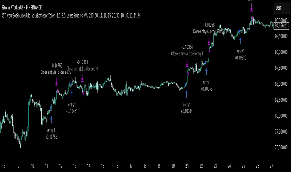
KST Strategy [Skyrexio]Overview
KST Strategy leverages Know Sure Thing (KST) indicator in conjunction with the Williams Alligator and Moving average to obtain the high probability setups. KST is used for for having the high probability to enter in the direction of a current trend when momentum is rising, Alligator is used as a short term trend filter, while Moving average approximates the long term trend and allows trades only in its direction. Also strategy has the additional optional filter on Choppiness Index which does not allow trades if market is choppy, above the user-specified threshold. Strategy has the user specified take profit and stop-loss numbers, but multiplied by Average True Range (ATR) value on the moment when trade is open. The strategy opens only long trades.
Unique Features
ATR based stop-loss and take profit. Instead of fixed take profit and stop-loss percentage strategy utilizes user chosen numbers multiplied by ATR for its calculation.
Configurable Trading Periods. Users can tailor the strategy to specific market windows, adapting to different market conditions.
Optional Choppiness Index filter. Strategy allows to choose if it will use the filter trades with Choppiness Index and set up its threshold.
Methodology
The strategy opens long trade when the following price met the conditions:
Close price is above the Alligator's jaw line
Close price is above the filtering Moving average
KST line of Know Sure Thing indicator shall cross over its signal line (details in justification of methodology)
If the Choppiness Index filter is enabled its value shall be less than user defined threshold
When the long trade is executed algorithm defines the stop-loss level as the low minus user defined number, multiplied by ATR at the trade open candle. Also it defines take profit with close price plus user defined number, multiplied by ATR at the trade open candle. While trade is in progress, if high price on any candle above the calculated take profit level or low price is below the calculated stop loss level, trade is closed.
Strategy settings
In the inputs window user can setup the following strategy settings:
ATR Stop Loss (by default = 1.5, number of ATRs to calculate stop-loss level)
ATR Take Profit (by default = 3.5, number of ATRs to calculate take profit level)
Filter MA Type (by default = Least Squares MA, type of moving average which is used for filter MA)
Filter MA Length (by default = 200, length for filter MA calculation)
Enable Choppiness Index Filter (by default = true, setting to choose the optional filtering using Choppiness index)
Choppiness Index Threshold (by default = 50, Choppiness Index threshold, its value shall be below it to allow trades execution)
Choppiness Index Length (by default = 14, length used in Choppiness index calculation)
KST ROC Length #1 (by default = 10, value used in KST indicator calculation, more information in Justification of Methodology)
KST ROC Length #2 (by default = 15, value used in KST indicator calculation, more information in Justification of Methodology)
KST ROC Length #3 (by default = 20, value used in KST indicator calculation, more information in Justification of Methodology)
KST ROC Length #4 (by default = 30, value used in KST indicator calculation, more information in Justification of Methodology)
KST SMA Length #1 (by default = 10, value used in KST indicator calculation, more information in Justification of Methodology)
KST SMA Length #2 (by default = 10, value used in KST indicator calculation, more information in Justification of Methodology)
KST SMA Length #3 (by default = 10, value used in KST indicator calculation, more information in Justification of Methodology)
KST SMA Length #4 (by default = 15, value used in KST indicator calculation, more information in Justification of Methodology)
KST Signal Line Length (by default = 10, value used in KST indicator calculation, more information in Justification of Methodology)
User can choose the optimal parameters during backtesting on certain price chart.
Justification of Methodology
Before understanding why this particular combination of indicator has been chosen let's briefly explain what is KST, Williams Alligator, Moving Average, ATR and Choppiness Index.
The KST (Know Sure Thing) is a momentum oscillator developed by Martin Pring. It combines multiple Rate of Change (ROC) values, smoothed over different timeframes, to identify trend direction and momentum strength. First of all, what is ROC? ROC (Rate of Change) is a momentum indicator that measures the percentage change in price between the current price and the price a set number of periods ago.
ROC = 100 * (Current Price - Price N Periods Ago) / Price N Periods Ago
In our case N is the KST ROC Length inputs from settings, here we will calculate 4 different ROCs to obtain KST value:
KST = ROC1_smooth × 1 + ROC2_smooth × 2 + ROC3_smooth × 3 + ROC4_smooth × 4
ROC1 = ROC(close, KST ROC Length #1), smoothed by KST SMA Length #1,
ROC2 = ROC(close, KST ROC Length #2), smoothed by KST SMA Length #2,
ROC3 = ROC(close, KST ROC Length #3), smoothed by KST SMA Length #3,
ROC4 = ROC(close, KST ROC Length #4), smoothed by KST SMA Length #4
Also for this indicator the signal line is calculated:
Signal = SMA(KST, KST Signal Line Length)
When the KST line rises, it indicates increasing momentum and suggests that an upward trend may be developing. Conversely, when the KST line declines, it reflects weakening momentum and a potential downward trend. A crossover of the KST line above its signal line is considered a buy signal, while a crossover below the signal line is viewed as a sell signal. If the KST stays above zero, it indicates overall bullish momentum; if it remains below zero, it points to bearish momentum. The KST indicator smooths momentum across multiple timeframes, helping to reduce noise and provide clearer signals for medium- to long-term trends.
Next, let’s discuss the short-term trend filter, which combines the Williams Alligator and Williams Fractals. Williams Alligator
Developed by Bill Williams, the Alligator is a technical indicator that identifies trends and potential market reversals. It consists of three smoothed moving averages:
Jaw (Blue Line): The slowest of the three, based on a 13-period smoothed moving average shifted 8 bars ahead.
Teeth (Red Line): The medium-speed line, derived from an 8-period smoothed moving average shifted 5 bars forward.
Lips (Green Line): The fastest line, calculated using a 5-period smoothed moving average shifted 3 bars forward.
When the lines diverge and align in order, the "Alligator" is "awake," signaling a strong trend. When the lines overlap or intertwine, the "Alligator" is "asleep," indicating a range-bound or sideways market. This indicator helps traders determine when to enter or avoid trades.
The next indicator is Moving Average. It has a lot of different types which can be chosen to filter trades and the Least Squares MA is used by default settings. Let's briefly explain what is it.
The Least Squares Moving Average (LSMA) — also known as Linear Regression Moving Average — is a trend-following indicator that uses the least squares method to fit a straight line to the price data over a given period, then plots the value of that line at the most recent point. It draws the best-fitting straight line through the past N prices (using linear regression), and then takes the endpoint of that line as the value of the moving average for that bar. The LSMA aims to reduce lag and highlight the current trend more accurately than traditional moving averages like SMA or EMA.
Key Features:
It reacts faster to price changes than most moving averages.
It is smoother and less noisy than short-term EMAs.
It can be used to identify trend direction, momentum, and potential reversal points.
ATR (Average True Range) is a volatility indicator that measures how much an asset typically moves during a given period. It was introduced by J. Welles Wilder and is widely used to assess market volatility, not direction.
To calculate it first of all we need to get True Range (TR), this is the greatest value among:
High - Low
abs(High - Previous Close)
abs(Low - Previous Close)
ATR = MA(TR, n) , where n is number of periods for moving average, in our case equals 14.
ATR shows how much an asset moves on average per candle/bar. A higher ATR means more volatility; a lower ATR means a calmer market.
The Choppiness Index is a technical indicator that quantifies whether the market is trending or choppy (sideways). It doesn't indicate trend direction — only the strength or weakness of a trend. Higher Choppiness Index usually approximates the sideways market, while its low value tells us that there is a high probability of a trend.
Choppiness Index = 100 × log10(ΣATR(n) / (MaxHigh(n) - MinLow(n))) / log10(n)
where:
ΣATR(n) = sum of the Average True Range over n periods
MaxHigh(n) = highest high over n periods
MinLow(n) = lowest low over n periods
log10 = base-10 logarithm
Now let's understand how these indicators work in conjunction and why they were chosen for this strategy. KST indicator approximates current momentum, when it is rising and KST line crosses over the signal line there is high probability that short term trend is reversing to the upside and strategy allows to take part in this potential move. Alligator's jaw (blue) line is used as an approximation of a short term trend, taking trades only above it we want to avoid trading against trend to increase probability that long trade is going to be winning.
Almost the same for Moving Average, but it approximates the long term trend, this is just the additional filter. If we trade in the direction of the long term trend we increase probability that higher risk to reward trade will hit the take profit. Choppiness index is the optional filter, but if it turned on it is used for approximating if now market is in sideways or in trend. On the range bounded market the potential moves are restricted. We want to decrease probability opening trades in such condition avoiding trades if this index is above threshold value.
When trade is open script sets the stop loss and take profit targets. ATR approximates the current volatility, so we can make a decision when to exit a trade based on current market condition, it can increase the probability that strategy will avoid the excessive stop loss hits, but anyway user can setup how many ATRs to use as a stop loss and take profit target. As was said in the Methodology stop loss level is obtained by subtracting number of ATRs from trade opening candle low, while take profit by adding to this candle's close.
Backtest Results
Operating window: Date range of backtests is 2023.01.01 - 2025.05.01. It is chosen to let the strategy to close all opened positions.
Commission and Slippage: Includes a standard Binance commission of 0.1% and accounts for possible slippage over 5 ticks.
Initial capital: 10000 USDT
Percent of capital used in every trade: 60%
Maximum Single Position Loss: -5.53%
Maximum Single Profit: +8.35%
Net Profit: +5175.20 USDT (+51.75%)
Total Trades: 120 (56.67% win rate)
Profit Factor: 1.747
Maximum Accumulated Loss: 1039.89 USDT (-9.1%)
Average Profit per Trade: 43.13 USDT (+0.6%)
Average Trade Duration: 27 hours
These results are obtained with realistic parameters representing trading conditions observed at major exchanges such as Binance and with realistic trading portfolio usage parameters.
How to Use
Add the script to favorites for easy access.
Apply to the desired timeframe and chart (optimal performance observed on 1h BTC/USDT).
Configure settings using the dropdown choice list in the built-in menu.
Set up alerts to automate strategy positions through web hook with the text: {{strategy.order.alert_message}}
Disclaimer:
Educational and informational tool reflecting Skyrexio commitment to informed trading. Past performance does not guarantee future results. Test strategies in a simulated environment before live implementation.
GQT GPT - Volume-based Support & Resistance Zones V2搞钱兔,搞钱是为了更好的生活。
Title: GQT GPT - Volume-based Support & Resistance Zones V2
Overview:
This strategy is implemented in PineScript v5 and is designed to identify key support and resistance zones based on volume-driven fractal analysis on a 1-hour timeframe. It computes fractal high points (for resistance) and fractal low points (for support) using volume moving averages and specific price action criteria. These zones are visually represented on the chart with customizable lines and zone fills.
Trading Logic:
• Entry: The strategy initiates a long position when the price crosses into the support zone (i.e., when the price drops into a predetermined support area).
• Exit: The long position is closed when the price enters the resistance zone (i.e., when the price rises into a predetermined resistance area).
• Time Frame: Trading signals are generated solely from the 1-hour chart. The strategy is only active within a specified start and end date.
• Note: Only long trades are executed; short selling is not part of the strategy.
Visualization and Parameters:
• Support/Resistance Zones: The zones are drawn based on calculated fractal values, with options to extend the lines to the right for easier tracking.
• Customization: Users can configure the appearance, such as line style (solid, dotted, dashed), line width, colors, and label positions.
• Volume Filtering: A volume moving average threshold is used to confirm the fractal signals, enhancing the reliability of the support and resistance levels.
• Alerts: The strategy includes alert conditions for when the price enters the support or resistance zones, allowing for timely notifications.
⸻
搞钱兔,搞钱是为了更好的生活。
标题: GQT GPT - 基于成交量的支撑与阻力区间 V2
概述:
本策略使用 PineScript v5 实现,旨在基于成交量驱动的分形分析,在1小时级别的图表上识别关键支撑与阻力区间。策略通过成交量移动平均线和特定的价格行为标准计算分形高点(阻力)和分形低点(支撑),并以自定义的线条和区间填充形式直观地显示在图表上。
交易逻辑:
• 进场条件: 当价格进入支撑区间(即价格跌入预设支撑区域)时,策略在没有持仓的情况下发出做多信号。
• 离场条件: 当价格进入阻力区间(即价格上升至预设阻力区域)时,持有多头头寸则会被平仓。
• 时间范围: 策略的信号仅基于1小时级别的图表,并且仅在指定的开始日期与结束日期之间生效。
• 备注: 本策略仅执行多头交易,不进行空头操作。
可视化与参数设置:
• 支撑/阻力区间: 根据计算得出的分形值绘制支撑与阻力线,可选择将线条延伸至右侧,便于后续观察。
• 自定义选项: 用户可以调整线条样式(实线、点线、虚线)、线宽、颜色及标签位置,以满足个性化需求。
• 成交量过滤: 策略使用成交量移动平均阈值来确认分形信号,提高支撑和阻力区间的有效性。
• 警报功能: 当价格进入支撑或阻力区间时,策略会触发警报条件,方便用户及时关注市场变化。
⸻

Quarterly Theory ICT 01 [TradingFinder] XAMD + Q1-Q4 Sessions🔵 Introduction
The Quarterly Theory ICT indicator is an advanced analytical system based on the concepts of ICT (Inner Circle Trader) and fractal time. It divides time into quarterly periods and accurately determines entry and exit points for trades by using the True Open as the starting point of each cycle. This system is applicable across various time frames including annual, monthly, weekly, daily, and even 90-minute sessions.
Time is divided into four quarters: in the first quarter (Q1), which is dedicated to the Accumulation phase, the market is in a consolidation state, laying the groundwork for a new trend; in the second quarter (Q2), allocated to the Manipulation phase (also known as Judas Swing), sudden price changes and false moves occur, marking the true starting point of a trend change; the third quarter (Q3) is dedicated to the Distribution phase, during which prices are broadly distributed and price volatility peaks; and the fourth quarter (Q4), corresponding to the Continuation/Reversal phase, either continues or reverses the previous trend.
By leveraging smart algorithms and technical analysis, this system identifies optimal price patterns and trading positions through the precise detection of stop-run and liquidity zones.
With the division of time into Q1 through Q4 and by incorporating key terms such as Quarterly Theory ICT, True Open, Accumulation, Manipulation (Judas Swing), Distribution, Continuation/Reversal, ICT, fractal time, smart algorithms, technical analysis, price patterns, trading positions, stop-run, and liquidity, this system enables traders to identify market trends and make informed trading decisions using real data and precise analysis.
♦ Important Note :
This indicator and the "Quarterly Theory ICT" concept have been developed based on material published in primary sources, notably the articles on Daye( traderdaye ) and Joshuuu . All copyright rights are reserved.
🔵 How to Use
The Quarterly Theory ICT strategy is built on dividing time into four distinct periods across various time frames such as annual, monthly, weekly, daily, and even 90-minute sessions. In this approach, time is segmented into four quarters, during which the phases of Accumulation, Manipulation (Judas Swing), Distribution, and Continuation/Reversal appear in a systematic and recurring manner.
The first segment (Q1) functions as the Accumulation phase, where the market consolidates and lays the foundation for future movement; the second segment (Q2) represents the Manipulation phase, during which prices experience sudden initial changes, and with the aid of the True Open concept, the real starting point of the market’s movement is determined; in the third segment (Q3), the Distribution phase takes place, where prices are widely dispersed and price volatility reaches its peak; and finally, the fourth segment (Q4) is recognized as the Continuation/Reversal phase, in which the previous trend either continues or reverses.
This strategy, by harnessing the concepts of fractal time and smart algorithms, enables precise analysis of price patterns across multiple time frames and, through the identification of key points such as stop-run and liquidity zones, assists traders in optimizing their trading positions. Utilizing real market data and dividing time into Q1 through Q4 allows for a comprehensive and multi-level technical analysis in which optimal entry and exit points are identified by comparing prices to the True Open.
Thus, by focusing on keywords like Quarterly Theory ICT, True Open, Accumulation, Manipulation, Distribution, Continuation/Reversal, ICT, fractal time, smart algorithms, technical analysis, price patterns, trading positions, stop-run, and liquidity, the Quarterly Theory ICT strategy acts as a coherent framework for predicting market trends and developing trading strategies.
🔵b]Settings
Cycle Display Mode: Determines whether the cycle is displayed on the chart or on the indicator panel.
Show Cycle: Enables or disables the display of the ranges corresponding to each quarter within the micro cycles (e.g., Q1/1, Q1/2, Q1/3, Q1/4, etc.).
Show Cycle Label: Toggles the display of textual labels for identifying the micro cycle phases (for example, Q1/1 or Q2/2).
Table Display Mode: Enables or disables the ability to display cycle information in a tabular format.
Show Table: Determines whether the table—which summarizes the phases (Q1 to Q4)—is displayed.
Show More Info: Adds additional details to the table, such as the name of the phase (Accumulation, Manipulation, Distribution, or Continuation/Reversal) or further specifics about each cycle.
🔵 Conclusion
Quarterly Theory ICT provides a fractal and recurring approach to analyzing price behavior by dividing time into four quarters (Q1, Q2, Q3, and Q4) and defining the True Open at the beginning of the second phase.
The Accumulation, Manipulation (Judas Swing), Distribution, and Continuation/Reversal phases repeat in each cycle, allowing traders to identify price patterns with greater precision across annual, monthly, weekly, daily, and even micro-level time frames.
Focusing on the True Open as the primary reference point enables faster recognition of potential trend changes and facilitates optimal management of trading positions. In summary, this strategy, based on ICT principles and fractal time concepts, offers a powerful framework for predicting future market movements, identifying optimal entry and exit points, and managing risk in various trading conditions.

Market Participation Index [PhenLabs]📊 Market Participation Index
Version: PineScript™ v6
📌 Description
Market Participation Index is a well-evolved statistical oscillator that constantly learns to develop by adapting to changing market behavior through the intricate mathematical modeling process. MPI combines different statistical approaches and Bayes’ probability theory of analysis to provide extensive insight into market participation and building momentum. MPI combines diverse statistical thinking principles of physics and information and marries them for subtle changes to occur in markets, levels to become influential as important price targets, and pattern divergences to unveil before it is visible by analytical methods in an old-fashioned methodology.
🚀 Points of Innovation:
Automatic market condition detection system with intelligent preset selection
Multi-statistical approach combining classical and advanced metrics
Fractal-based divergence system with quality scoring
Adaptive threshold calculation using statistical properties of current market
🚨 Important🚨
The ‘Auto’ mode intelligently selects the optimal preset based on real-time market conditions, if the visualization does not appear to the best of your liking then select the option in parenthesis next to the auto mode on the label in the oscillator in the settings panel.
🔧 Core Components
Statistical Foundation: Multiple statistical measures combined with weighted approach
Market Condition Analysis: Real-time detection of market states (trending, ranging, volatile)
Change Point Detection: Bayesian analysis for finding significant market structure shifts
Divergence System: Fractal-based pattern detection with quality assessment
Adaptive Visualization: Dynamic color schemes with context-appropriate settings
🔥 Key Features
The indicator provides comprehensive market analysis through:
Multi-statistical Oscillator: Combines Z-score, MAD, and fractal dimensions
Advanced Statistical Components: Includes skewness, kurtosis, and entropy analysis
Auto-preset System: Automatically selects optimal settings for current conditions
Fractal Divergence Analysis: Detects and grades quality of divergence patterns
Adaptive Thresholds: Dynamically adjusts overbought/oversold levels
🎨 Visualization
Color-coded Oscillator: Gradient-filled oscillator line showing intensity
Divergence Markings: Clear visualization of bullish and bearish divergences
Threshold Lines: Dynamic or fixed overbought/oversold levels
Preset Information: On-chart display of current market conditions
Multiple Color Schemes: Modern, Classic, Monochrome, and Neon themes
Classic
Modern
Monochrome
Neon
📖 Usage Guidelines
The indicator offers several customization options:
Market Condition Settings:
Preset Mode: Choose between Auto-detection or specific market condition presets
Color Theme: Select visual theme matching your chart style
Divergence Labels: Choose whether or not you’d like to see the divergence
✅ Best Use Cases:
Identify potential market reversals through statistical divergences
Detect changes in market structure before price confirmation
Filter trades based on current market condition (trending vs. ranging)
Find optimal entry and exit points using adaptive thresholds
Monitor shifts in market participation and momentum
⚠️ Limitations
Requires sufficient historical data for accurate statistical analysis
Auto-detection may lag during rapid market condition changes
Advanced statistical calculations have higher computational requirements
Manual preset selection may be required in certain transitional markets
💡 What Makes This Unique
Statistical Depth: Goes beyond traditional indicators with advanced statistical measures
Adaptive Intelligence: Automatically adjusts to current market conditions
Bayesian Analysis: Identifies statistically significant change points in market structure
Multi-factor Approach: Combines multiple statistical dimensions for confirmation
Fractal Divergence System: More robust than traditional divergence detection methods
🔬 How It Works
The indicator processes market data through four main components:
Market Condition Analysis:
Evaluates trend strength, volatility, and price patterns
Automatically selects optimal preset parameters
Adapts sensitivity based on current conditions
Statistical Oscillator:
Combines multiple statistical measures with weights
Normalizes values to consistent scale
Applies adaptive smoothing
Advanced Statistical Analysis:
Calculates higher-order statistical moments
Applies information-theoretic measures
Detects distribution anomalies
Divergence Detection:
Uses fractal theory to identify pivot points
Detects and scores divergence quality
Filters signals based on current market phase
💡 Note:
The Market Participation Index performs optimally when used across multiple timeframes for confirmation. Its statistical foundation makes it particularly valuable during market transitions and periods of changing volatility, where traditional indicators often fail to provide clear signals.
G-FRAMA | QuantEdgeBIntroducing G-FRAMA by QuantEdgeB
Overview
The Gaussian FRAMA (G-FRAMA) is an adaptive trend-following indicator that leverages the power of Fractal Adaptive Moving Averages (FRAMA), enhanced with a Gaussian filter for noise reduction and an ATR-based dynamic band for trade signal confirmation. This combination results in a highly responsive moving average that adapts to market volatility while filtering out insignificant price movements.
_____
1. Key Features
- 📈 Gaussian Smoothing – Utilizes a Gaussian filter to refine price input, reducing short-term noise while maintaining responsiveness.
- 📊 Fractal Adaptive Moving Average (FRAMA) – A self-adjusting moving average that adapts its sensitivity to market trends.
- 📉 ATR-Based Volatility Bands – Dynamic upper and lower bands based on the Average True Range (ATR), improving signal reliability.
- ⚡ Adaptive Trend Signals – Automatically detects shifts in market structure by evaluating price in relation to FRAMA and its ATR bands.
_____
2. How It Works
- Gaussian Filtering
The Gaussian function preprocesses the price data, giving more weight to recent values and smoothing fluctuations. This reduces whipsaws and allows the FRAMA calculation to focus on meaningful trend developments.
- Fractal Adaptive Moving Average (FRAMA)
Unlike traditional moving averages, FRAMA uses fractal dimension calculations to adjust its smoothing factor dynamically. In trending markets, it reacts faster, while in sideways conditions, it reduces sensitivity, filtering out noise.
- ATR-Based Volatility Bands
ATR is applied to determine upper and lower thresholds around FRAMA:
- 🔹 Long Condition: Price closes above FRAMA + ATR*Multiplier
- 🔻 Short Condition: Price closes below FRAMA - ATR
This setup ensures entries are volatility-adjusted, preventing premature exits or false signals in choppy conditions.
_____
3. Use Cases
✔ Adaptive Trend Trading – Automatically adjusts to different market conditions, making it ideal for both short-term and long-term traders.
✔ Noise-Filtered Entries – Gaussian smoothing prevents false breakouts, allowing for cleaner entries.
✔ Breakout & Volatility Strategies – The ATR bands confirm valid price movements, reducing false signals.
✔ Smooth but Aggressive Shorts – While the indicator is smooth in overall trend detection, it reacts aggressively to downside moves, making it well-suited for traders focusing on short opportunities.
_____
4. Customization Options
- Gaussian Filter Settings – Adjust length & sigma to fine-tune the smoothness of the input price. (Default: Gaussian length = 4, Gaussian sigma = 2.0, Gaussian source = close)
- FRAMA Length & Limits – Modify how quickly FRAMA reacts to price changes.(Default: Base FRAMA = 20, Upper FRAMA Limit = 8, Lower FRAMA Limit = 40)
- ATR Multiplier – Control how wide the volatility bands are for long/short entries.(Default: ATR Length = 14, ATR Multiplier = 1.9)
- Color Themes – Multiple visual styles to match different trading environments.
_____
Conclusion
The G-FRAMA is an intelligent trend-following tool that combines the adaptability of FRAMA with the precision of Gaussian filtering and volatility-based confirmation. It is versatile across different timeframes and asset classes, offering traders an edge in trend detection and trade execution.
____
🔹 Disclaimer: Past performance is not indicative of future results. No trading strategy can guarantee success in financial markets.
🔹 Strategic Advice: Always backtest, optimize, and align parameters with your trading objectives and risk tolerance before live trading.
Trend Trader-Remastered StrategyOfficial Strategy for Trend Trader - Remastered
Indicator: Trend Trader-Remastered (TTR)
Overview:
The Trend Trader-Remastered is a refined and highly sophisticated implementation of the Parabolic SAR designed to create strategic buy and sell entry signals, alongside precision take profit and re-entry signals based on marked Bill Williams (BW) fractals. Built with a deep emphasis on clarity and accuracy, this indicator ensures that only relevant and meaningful signals are generated, eliminating any unnecessary entries or exits.
Please check the indicator details and updates via the link above.
Important Disclosure:
My primary objective is to provide realistic strategies and a code base for the TradingView Community. Therefore, the default settings of the strategy version of the indicator have been set to reflect realistic world trading scenarios and best practices.
Key Features:
Strategy execution date&time range.
Take Profit Reduction Rate: The percentage of progressive reduction on active position size for take profit signals.
Example:
TP Reduce: 10%
Entry Position Size: 100
TP1: 100 - 10 = 90
TP2: 90 - 9 = 81
Re-Entry When Rate: The percentage of position size on initial entry of the signal to determine re-entry.
Example:
RE When: 50%
Entry Position Size: 100
Re-Entry Condition: Active Position Size < 50
Re-Entry Fill Rate: The percentage of position size on initial entry of the signal to be completed.
Example:
RE Fill: 75%
Entry Position Size: 100
Active Position Size: 50
Re-Entry Order Size: 25
Final Active Position Size:75
Important: Even RE When condition is met, the active position size required to drop below RE Fill rate to trigger re-entry order.
Key Points:
'Process Orders on Close' is enabled as Take Profit and Re-Entry signals must be executed on candle close.
'Calculate on Every Tick' is enabled as entry signals are required to be executed within candle time.
'Initial Capital' has been set to 10,000 USD.
'Default Quantity Type' has been set to 'Percent of Equity'.
'Default Quantity' has been set to 10% as the best practice of investing 10% of the assets.
'Currency' has been set to USD.
'Commission Type' has been set to 'Commission Percent'
'Commission Value' has been set to 0.05% to reflect the most realistic results with a common taker fee value.
Market DirectionThe "Market Direction" indicator combines four advanced sub-indicators to provide a comprehensive and multi-dimensional analysis of market trends, momentum, and potential reversals. This innovative approach leverages different aspects of price action, volume, and market sentiment, offering traders an in-depth view of market conditions.
1. Fractal Indicator: Multi-Scale Price Action Analysis
The Fractal Indicator identifies significant highs and lows over six different pivot lengths, offering a nuanced view of price action across multiple timeframes. By comparing distances from current closing prices to these key fractal points, the indicator determines potential trend reversals and market direction. This approach enables traders to adapt their strategies to various market conditions, capturing both short-term fluctuations and long-term trends.
2. Volume MACD Indicator: Enhanced Market Momentum
The Volume MACD Indicator goes beyond traditional MACD analysis by incorporating volume-weighted movement and the structural attributes of candlesticks (such as body length and wicks). This hybrid model offers a more comprehensive understanding of market momentum by integrating both price action and trading volume. The use of Smoothed Moving Averages (SMMA) reduces noise and ensures more stable signals, helping traders focus on sustainable trends and longer-term investment opportunities.
3. Cumulative Volume Momentum Indicator: Volume Dynamics Insight
The Cumulative Volume Momentum Indicator evaluates the momentum of cumulative buying and selling volumes, offering a clear picture of market strength and potential reversals. By comparing the relationship between open, close, high, and low prices, and applying a MACD approach to these volume dynamics, this indicator helps traders identify momentum shifts that often precede price movements. The visualization through histograms adds clarity to bullish and bearish volume momentum, enhancing decision-making in volatile markets.
4. POC-Price Momentum Indicator: Market Depth and Sentiment
The POC-Price Momentum Indicator assesses the difference between the Point of Control (POC) and closing prices, providing insights into underlying market sentiment. Positive differences indicate a buildup of upward momentum, while negative differences suggest a bearish tilt. By calculating moving averages of these differences, the indicator highlights the strength and sustainability of ongoing trends, helping traders align their strategies with the broader market direction.
Unified Rating for Confirming Market Direction
The "Market Direction" indicator consolidates the outputs of these four sub-indicators into a single, aggregated sentiment score. This score helps traders confirm the prevailing market trend by weighing the combined insights from fractal analysis, volume momentum, price action, and POC dynamics. A positive score suggests a bullish market, while a negative score indicates bearish conditions.

Six PillarsGeneral Overview
The "Six Pillars" indicator is a comprehensive trading tool that combines six different technical analysis methods to provide a holistic view of market conditions.
These six pillars are:
Trend
Momentum
Directional Movement (DM)
Stochastic
Fractal
On-Balance Volume (OBV)
The indicator calculates the state of each pillar and presents them in an easy-to-read table format. It also compares the current timeframe with a user-defined comparison timeframe to offer a multi-timeframe analysis.
A key feature of this indicator is the Confluence Strength meter. This unique metric quantifies the overall agreement between the six pillars across both timeframes, providing a score out of 100. A higher score indicates stronger agreement among the pillars, suggesting a more reliable trading signal.
I also included a visual cue in the form of candle coloring. When all six pillars agree on a bullish or bearish direction, the candle is colored green or red, respectively. This feature allows traders to quickly identify potential high-probability trade setups.
The Six Pillars indicator is designed to work across multiple timeframes, offering a comparison between the current timeframe and a user-defined comparison timeframe. This multi-timeframe analysis provides traders with a more comprehensive understanding of market dynamics.
Origin and Inspiration
The Six Pillars indicator was inspired by the work of Dr. Barry Burns, author of "Trend Trading for Dummies" and his concept of "5 energies." (Trend, Momentum, Cycle, Support/Resistance, Scale) I was intrigued by Dr. Burns' approach to analyzing market dynamics and decided to put my own twist upon his ideas.
Comparing the Six Pillars to Dr. Burns' 5 energies, you'll notice I kept Trend and Momentum, but I swapped out Cycle, Support/Resistance, and Scale for Directional Movement, Stochastic, Fractal, and On-Balance Volume. These changes give you a more dynamic view of market strength, potential reversals, and volume confirmation all in one package.
What Makes This Indicator Unique
The standout feature of the Six Pillars indicator is its Confluence Strength meter. This feature calculates the overall agreement between the six pillars, providing traders with a clear, numerical representation of signal strength.
The strength is calculated by considering the state of each pillar in both the current and comparison timeframes, resulting in a score out of 100.
Here's how it calculates the strength:
It considers the state of each pillar in both the current timeframe and the comparison timeframe.
For each pillar, the absolute value of its state is taken. This means that both strongly bullish (2) and strongly bearish (-2) states contribute equally to the strength.
The absolute values for all six pillars are summed up for both timeframes, resulting in two sums: current_sum and alternate_sum.
These sums are then added together to get a total_sum.
The total_sum is divided by 24 (the maximum possible sum if all pillars were at their strongest states in both timeframes) and multiplied by 100 to get a percentage.
The result is rounded to the nearest integer and capped at a minimum of 1.
This calculation method ensures that the Confluence Strength meter takes into account not only the current timeframe but also the comparison timeframe, providing a more robust measure of overall market sentiment. The resulting score, ranging from 1 to 100, gives traders a clear and intuitive measure of how strongly the pillars agree, with higher scores indicating stronger potential signals.
This approach to measuring signal strength is unique in that it doesn't just rely on a single aspect of price action or volume. Instead, it takes into account multiple factors, providing a more robust and reliable indication of potential market moves. The higher the Confluence Strength score, the more confident traders can be in the signal.
The Confluence Strength meter helps traders in several ways:
It provides a quick and easy way to gauge the overall market sentiment.
It helps prioritize potential trades by identifying the strongest signals.
It can be used as a filter to avoid weaker setups and focus on high-probability trades.
It offers an additional layer of confirmation for other trading strategies or indicators.
By combining the Six Pillars analysis with the Confluence Strength meter, I've created a powerful tool that not only identifies potential trading opportunities but also quantifies their strength, giving traders a significant edge in their decision-making process.
How the Pillars Work (What Determines Bullish or Bearish)
While developing this indicator, I selected and configured six key components that work together to provide a comprehensive view of market conditions. Each pillar is set up to complement the others, creating a synergistic effect that offers traders a more nuanced understanding of price action and volume.
Trend Pillar: Based on two Exponential Moving Averages (EMAs) - a fast EMA (8 period) and a slow EMA (21 period). It determines the trend by comparing these EMAs, with stronger trends indicated when the fast EMA is significantly above or below the slow EMA.
Directional Movement (DM) Pillar: Utilizes the Average Directional Index (ADX) with a default period of 14. It measures trend strength, with values above 25 indicating a strong trend. It also considers the Positive and Negative Directional Indicators (DI+ and DI-) to determine trend direction.
Momentum Pillar: Uses the Moving Average Convergence Divergence (MACD) with customizable fast (12), slow (26), and signal (9) lengths. It compares the MACD line to the signal line to determine momentum strength and direction.
Stochastic Pillar: Employs the Stochastic oscillator with a default period of 13. It identifies overbought conditions (above 80) and oversold conditions (below 20), with intermediate zones between 60-80 and 20-40.
Fractal Pillar: Uses Williams' Fractal indicator with a default period of 3. It identifies potential reversal points by looking for specific high and low patterns over the given period.
On-Balance Volume (OBV) Pillar: Incorporates On-Balance Volume with three EMAs - short (3), medium (13), and long (21) periods. It assesses volume trends by comparing these EMAs.
Each pillar outputs a state ranging from -2 (strongly bearish) to 2 (strongly bullish), with 0 indicating a neutral state. This standardized output allows for easy comparison and aggregation of signals across all pillars.
Users can customize various parameters for each pillar, allowing them to fine-tune the indicator to their specific trading style and market conditions. The multi-timeframe comparison feature also allows users to compare pillar states between the current timeframe and a user-defined comparison timeframe, providing additional context for decision-making.
Design
From a design standpoint, I've put considerable effort into making the Six Pillars indicator visually appealing and user-friendly. The clean and minimalistic design is a key feature that sets this indicator apart.
I've implemented a sleek table layout that displays all the essential information in a compact and organized manner. The use of a dark background (#030712) for the table creates a sleek look that's easy on the eyes, especially during extended trading sessions.
The overall design philosophy focuses on presenting complex information in a simple, intuitive format, allowing traders to make informed decisions quickly and efficiently.
The color scheme is carefully chosen to provide clear visual cues:
White text for headers ensures readability
Green (#22C55E) for bullish signals
Blue (#3B82F6) for neutral states
Red (#EF4444) for bearish signals
This color coding extends to the candle coloring, making it easy to spot when all pillars agree on a bullish or bearish outlook.
I've also incorporated intuitive symbols (↑↑, ↑, →, ↓, ↓↓) to represent the different states of each pillar, allowing for quick interpretation at a glance.
The table layout is thoughtfully organized, with clear sections for the current and comparison timeframes. The Confluence Strength meter is prominently displayed, providing traders with an immediate sense of signal strength.
To enhance usability, I've added tooltips to various elements, offering additional information and explanations when users hover over different parts of the indicator.
How to Use This Indicator
The Six Pillars indicator is a versatile tool that can be used for various trading strategies. Here are some general usage guidelines and specific scenarios:
General Usage Guidelines:
Pay attention to the Confluence Strength meter. Higher values indicate stronger agreement among the pillars and potentially more reliable signals.
Use the multi-timeframe comparison to confirm signals across different time horizons.
Look for alignment between the current timeframe and comparison timeframe pillars for stronger signals.
One of the strengths of this indicator is it can let you know when markets are sideways – so in general you can know to avoid entering when the Confluence Strength is low, indicating disagreement among the pillars.
Customization Options
The Six Pillars indicator offers a wide range of customization options, allowing traders to tailor the tool to their specific needs and trading style. Here are the key customizable elements:
Comparison Timeframe:
Users can select any timeframe for comparison with the current timeframe, providing flexibility in multi-timeframe analysis.
Trend Pillar:
Fast EMA Period: Adjustable for quicker or slower trend identification
Slow EMA Period: Can be modified to capture longer-term trends
Momentum Pillar:
MACD Fast Length
MACD Slow Length
MACD Signal Length These can be adjusted to fine-tune momentum sensitivity
DM Pillar:
ADX Period: Customizable to change the lookback period for trend strength measurement
ADX Threshold: Adjustable to define what constitutes a strong trend
Stochastic Pillar:
Stochastic Period: Can be modified to change the sensitivity of overbought/oversold readings
Fractal Pillar:
Fractal Period: Adjustable to identify potential reversal points over different timeframes
OBV Pillar:
Short OBV EMA
Medium OBV EMA
Long OBV EMA These periods can be customized to analyze volume trends over different timeframes
These customization options allow traders to experiment with different settings to find the optimal configuration for their trading strategy and market conditions. The flexibility of the Six Pillars indicator makes it adaptable to various trading styles and market environments.

Machine Learning: Optimal RSI [YinYangAlgorithms]This Indicator, will rate multiple different lengths of RSIs to determine which RSI to RSI MA cross produced the highest profit within the lookback span. This ‘Optimal RSI’ is then passed back, and if toggled will then be thrown into a Machine Learning calculation. You have the option to Filter RSI and RSI MA’s within the Machine Learning calculation. What this does is, only other Optimal RSI’s which are in the same bullish or bearish direction (is the RSI above or below the RSI MA) will be added to the calculation.
You can either (by default) use a Simple Average; which is essentially just a Mean of all the Optimal RSI’s with a length of Machine Learning. Or, you can opt to use a k-Nearest Neighbour (KNN) calculation which takes a Fast and Slow Speed. We essentially turn the Optimal RSI into a MA with different lengths and then compare the distance between the two within our KNN Function.
RSI may very well be one of the most used Indicators for identifying crucial Overbought and Oversold locations. Not only that but when it crosses its Moving Average (MA) line it may also indicate good locations to Buy and Sell. Many traders simply use the RSI with the standard length (14), however, does that mean this is the best length?
By using the length of the top performing RSI and then applying some Machine Learning logic to it, we hope to create what may be a more accurate, smooth, optimal, RSI.
Tutorial:
This is a pretty zoomed out Perspective of what the Indicator looks like with its default settings (except with Bollinger Bands and Signals disabled). If you look at the Tables above, you’ll notice, currently the Top Performing RSI Length is 13 with an Optimal Profit % of: 1.00054973. On its default settings, what it does is Scan X amount of RSI Lengths and checks for when the RSI and RSI MA cross each other. It then records the profitability of each cross to identify which length produced the overall highest crossing profitability. Whichever length produces the highest profit is then the RSI length that is used in the plots, until another length takes its place. This may result in what we deem to be the ‘Optimal RSI’ as it is an adaptive RSI which changes based on performance.
In our next example, we changed the ‘Optimal RSI Type’ from ‘All Crossings’ to ‘Extremity Crossings’. If you compare the last two examples to each other, you’ll notice some similarities, but overall they’re quite different. The reason why is, the Optimal RSI is calculated differently. When using ‘All Crossings’ everytime the RSI and RSI MA cross, we evaluate it for profit (short and long). However, with ‘Extremity Crossings’, we only evaluate it when the RSI crosses over the RSI MA and RSI <= 40 or RSI crosses under the RSI MA and RSI >= 60. We conclude the crossing when it crosses back on its opposite of the extremity, and that is how it finds its Optimal RSI.
The way we determine the Optimal RSI is crucial to calculating which length is currently optimal.
In this next example we have zoomed in a bit, and have the full default settings on. Now we have signals (which you can set alerts for), for when the RSI and RSI MA cross (green is bullish and red is bearish). We also have our Optimal RSI Bollinger Bands enabled here too. These bands allow you to see where there may be Support and Resistance within the RSI at levels that aren’t static; such as 30 and 70. The length the RSI Bollinger Bands use is the Optimal RSI Length, allowing it to likewise change in correlation to the Optimal RSI.
In the example above, we’ve zoomed out as far as the Optimal RSI Bollinger Bands go. You’ll notice, the Bollinger Bands may act as Support and Resistance locations within and outside of the RSI Mid zone (30-70). In the next example we will highlight these areas so they may be easier to see.
Circled above, you may see how many times the Optimal RSI faced Support and Resistance locations on the Bollinger Bands. These Bollinger Bands may give a second location for Support and Resistance. The key Support and Resistance may still be the 30/50/70, however the Bollinger Bands allows us to have a more adaptive, moving form of Support and Resistance. This helps to show where it may ‘bounce’ if it surpasses any of the static levels (30/50/70).
Due to the fact that this Indicator may take a long time to execute and it can throw errors for such, we have added a Setting called: Adjust Optimal RSI Lookback and RSI Count. This settings will automatically modify the Optimal RSI Lookback Length and the RSI Count based on the Time Frame you are on and the Bar Indexes that are within. For instance, if we switch to the 1 Hour Time Frame, it will adjust the length from 200->90 and RSI Count from 30->20. If this wasn’t adjusted, the Indicator would Timeout.
You may however, change the Setting ‘Adjust Optimal RSI Lookback and RSI Count’ to ‘Manual’ from ‘Auto’. This will give you control over the ‘Optimal RSI Lookback Length’ and ‘RSI Count’ within the Settings. Please note, it will likely take some “fine tuning” to find working settings without the Indicator timing out, but there are definitely times you can find better settings than our ‘Auto’ will create; especially on higher Time Frames. The Minimum our ‘Auto’ will create is:
Optimal RSI Lookback Length: 90
RSI Count: 20
The Maximum it will create is:
Optimal RSI Lookback Length: 200
RSI Count: 30
If there isn’t much bar index history, for instance, if you’re on the 1 Day and the pair is BTC/USDT you’ll get < 4000 Bar Indexes worth of data. For this reason it is possible to manually increase the settings to say:
Optimal RSI Lookback Length: 500
RSI Count: 50
But, please note, if you make it too high, it may also lead to inaccuracies.
We will conclude our Tutorial here, hopefully this has given you some insight as to how calculating our Optimal RSI and then using it within Machine Learning may create a more adaptive RSI.
Settings:
Optimal RSI:
Show Crossing Signals: Display signals where the RSI and RSI Cross.
Show Tables: Display Information Tables to show information like, Optimal RSI Length, Best Profit, New Optimal RSI Lookback Length and New RSI Count.
Show Bollinger Bands: Show RSI Bollinger Bands. These bands work like the TDI Indicator, except its length changes as it uses the current RSI Optimal Length.
Optimal RSI Type: This is how we calculate our Optimal RSI. Do we use all RSI and RSI MA Crossings or just when it crosses within the Extremities.
Adjust Optimal RSI Lookback and RSI Count: Auto means the script will automatically adjust the Optimal RSI Lookback Length and RSI Count based on the current Time Frame and Bar Index's on chart. This will attempt to stop the script from 'Taking too long to Execute'. Manual means you have full control of the Optimal RSI Lookback Length and RSI Count.
Optimal RSI Lookback Length: How far back are we looking to see which RSI length is optimal? Please note the more bars the lower this needs to be. For instance with BTC/USDT you can use 500 here on 1D but only 200 for 15 Minutes; otherwise it will timeout.
RSI Count: How many lengths are we checking? For instance, if our 'RSI Minimum Length' is 4 and this is 30, the valid RSI lengths we check is 4-34.
RSI Minimum Length: What is the RSI length we start our scans at? We are capped with RSI Count otherwise it will cause the Indicator to timeout, so we don't want to waste any processing power on irrelevant lengths.
RSI MA Length: What length are we using to calculate the optimal RSI cross' and likewise plot our RSI MA with?
Extremity Crossings RSI Backup Length: When there is no Optimal RSI (if using Extremity Crossings), which RSI should we use instead?
Machine Learning:
Use Rational Quadratics: Rationalizing our Close may be beneficial for usage within ML calculations.
Filter RSI and RSI MA: Should we filter the RSI's before usage in ML calculations? Essentially should we only use RSI data that are of the same type as our Optimal RSI? For instance if our Optimal RSI is Bullish (RSI > RSI MA), should we only use ML RSI's that are likewise bullish?
Machine Learning Type: Are we using a Simple ML Average, KNN Mean Average, KNN Exponential Average or None?
KNN Distance Type: We need to check if distance is within the KNN Min/Max distance, which distance checks are we using.
Machine Learning Length: How far back is our Machine Learning going to keep data for.
k-Nearest Neighbour (KNN) Length: How many k-Nearest Neighbours will we account for?
Fast ML Data Length: What is our Fast ML Length? This is used with our Slow Length to create our KNN Distance.
Slow ML Data Length: What is our Slow ML Length? This is used with our Fast Length to create our KNN Distance.
If you have any questions, comments, ideas or concerns please don't hesitate to contact us.
HAPPY TRADING!
IPDA Standard Deviations [DexterLab x TFO x toodegrees]> Introduction and Acknowledgements
The IPDA Standard Deviations tool encompasses the Time and price relationship as studied by @TraderDext3r .
I am not the creator of this Theory, and I do not hold the answers to all the questions you may have; I suggest you to study it from Dexter's tweets, videos, and material.
This tool was born from a collaboration between @TraderDext3r, @tradeforopp and I, with the objective of bringing a comprehensive IPDA Standard Deviations tool to Tradingview.
> Tool Description
This is purely a graphical aid for traders to be able to quickly determine Fractal IPDA Time Windows, and trace the potential Standard Deviations of the moves at their respective high and low extremes.
The disruptive value of this tool is that it allows traders to save Time by automatically adapting the Time Windows based on the current chart's Timeframe, as well as providing customizations to filter and focus on the appropriate Standard Deviations.
> IPDA Standard Deviations by TraderDext3r
The underlying idea is based on the Interbank Price Delivery Algorithm's lookback windows on the daily chart as taught by the Inner Circle Trader:
IPDA looks at the past three months of price action to determine how to deliver price in the future.
Additionally, the ICT concept of projecting specific manipulation moves prior to large displacement upwards/downwards is used to navigate and interpret the priorly mentioned displacement move. We pay attention to specific Standard Deviations based on the current environment and overall narrative.
Dexter being one of the most prominent Inner Circle Trader students, harnessed the fractal nature of price to derive fractal IPDA Lookback Time Windows for lower Timeframes, and studied the behaviour of price at specific Deviations.
For Example:
The -1 to -2 area can initiate an algorithmic retracement before continuation.
The -2 to -2.5 area can initiate an algorithmic retracement before continuation, or a Smart Money Reversal.
The -4 area should be seen as the ultimate objective, or the level at which the displacement will slow down.
Given that these ideas stem from ICT's concepts themselves, they are to be used hand in hand with all other ICT Concepts (PD Array Matrix, PO3, Institutional Price Levels, ...).
> Fractal IPDA Time Windows
The IPDA Lookbacks Types identified by Dexter are as follows:
Monthly – 1D Chart: one widow per Month, highlighting the past three Months.
Weekly – 4H to 8H Chart: one window per Week, highlighting the past three Weeks.
Daily – 15m to 1H Chart: one window per Day, highlighting the past three Days.
Intraday – 1m to 5m Chart: one window per 4 Hours highlighting the past 12 Hours.
Inside these three respective Time Windows, the extreme High and Low will be identified, as well as the prior opposing short term market structure point. These represent the anchors for the Standard Deviation Projections.
> Tool Settings
The User is able to plot any type of Standard Deviation they want by inputting them in the settings, in their own line of the text box. They will always be plotted from the Time Windows extremes.
As previously mentioned, the User is also able to define their own Timeframe intervals for the respective IPDA Lookback Types. The specific Timeframes on which the different Lookback Types are plotted are edge-inclusive. In case of an overlap, the higher Timeframe Lookback will be prioritized.
Finally the User is able to filter and remove Standard Deviations in two ways:
"Remove Once Invalidated" will automatically delete a Deviation once its outer anchor extreme is traded through.
Manual Toggles will allow to remove the Upward or Downward Deviation of each Time Window at the discretion of the User.
Major shoutout to Dexter and TFO for their Time, it was a pleasure to collaborate and create this tool with them.
GLGT!

mentfx Triple MThis indicator colors the wick of a candle on any timeframe based on whether the following rules are met:
A colored wick below a candle indicates that the candles low was lower than the previous candles low, and the body of the candle closed above the previous candles low.
A colored wick above a candle indicates that the candles high was higher than the previous candles high, and the body of the candle closed below the previous candles high.
The idea behind this indicator is to fractally see a distribution (colored wick above a candle) or an accumulation (colored wick below a candle) as a confirmation once you have established a directional trend or turning point. This indicator will color any wick that meets these conditions. This indicator is meant more so as an entry confirmation, coupling it with your understanding of turning points, or likely points that price will continue in a direction - this can provide a nice confirmation.

JFD-Adaptive, GKYZ-Filtered KAMA [Loxx]JFD-Adaptive, GKYZ-Filtered KAMA is a Kaufman Adaptive Moving Average with the option to make it Jurik Fractal Dimension Adaptive. This also includes a Garman-Klass-Yang-Zhang Historical Volatility Filter to reduce noise.
What is KAMA?
Developed by Perry Kaufman, Kaufman's Adaptive Moving Average ( KAMA ) is a moving average designed to account for market noise or volatility . KAMA will closely follow prices when the price swings are relatively small and the noise is low. KAMA will adjust when the price swings widen and follow prices from a greater distance. This trend-following indicator can be used to identify the overall trend, time turning points and filter price movements.
What is Jurik Fractal Dimension?
There is a weak and a strong way to measure the random quality of a time series.
The weak way is to use the random walk index ( RWI ). You can download it from the Omega web site. It makes the assumption that the market is moving randomly with an average distance D per move and proposes an amount the market should have changed over N bars of time. If the market has traveled less, then the action is considered random, otherwise it's considered trending.
The problem with this method is that taking the average distance is valid for a Normal (Gaussian) distribution of price activity. However, price action is rarely Normal, with large price jumps occuring much more frequently than a Normal distribution would expect. Consequently, big jumps throw the RWI way off, producing invalid results.
The strong way is to not make any assumption regarding the distribution of price changes and, instead, measure the fractal dimension of the time series. Fractal Dimension requires a lot of data to be accurate. If you are trading 30 minute bars, use a multi-chart where this indicator is running on 5 minute bars and you are trading on 30 minute bars.
What is Garman-Klass-Yang-Zhang Historical Volatility?
Yang and Zhang derived an extension to the Garman Klass historical volatility estimator that allows for opening jumps. It assumes Brownian motion with zero drift. This is currently the preferred version of open-high-low-close volatility estimator for zero drift and has an efficiency of 8 times the classic close-to-close estimator. Note that when the drift is nonzero, but instead relative large to the volatility , this estimator will tend to overestimate the volatility . The Garman-Klass-Yang-Zhang Historical Volatility calculation is as follows:
GKYZHV = sqrt((Z/n) * sum((log(open(k)/close( k-1 )))^2 + (0.5*(log(high(k)/low(k)))^2) - (2*log(2) - 1)*(log(close(k)/open(2:end)))^2))
Included
Alerts
Signals
Loxx's Expanded Source Types
Bar coloring