Markov Chain [3D] | FractalystWhat exactly is a Markov Chain?
This indicator uses a Markov Chain model to analyze, quantify, and visualize the transitions between market regimes (Bull, Bear, Neutral) on your chart. It dynamically detects these regimes in real-time, calculates transition probabilities, and displays them as animated 3D spheres and arrows, giving traders intuitive insight into current and future market conditions.
How does a Markov Chain work, and how should I read this spheres-and-arrows diagram?
Think of three weather modes: Sunny, Rainy, Cloudy.
Each sphere is one mode. The loop on a sphere means “stay the same next step” (e.g., Sunny again tomorrow).
The arrows leaving a sphere show where things usually go next if they change (e.g., Sunny moving to Cloudy).
Some paths matter more than others. A more prominent loop means the current mode tends to persist. A more prominent outgoing arrow means a change to that destination is the usual next step.
Direction isn’t symmetric: moving Sunny→Cloudy can behave differently than Cloudy→Sunny.
Now relabel the spheres to markets: Bull, Bear, Neutral.
Spheres: market regimes (uptrend, downtrend, range).
Self‑loop: tendency for the current regime to continue on the next bar.
Arrows: the most common next regime if a switch happens.
How to read: Start at the sphere that matches current bar state. If the loop stands out, expect continuation. If one outgoing path stands out, that switch is the typical next step. Opposite directions can differ (Bear→Neutral doesn’t have to match Neutral→Bear).
What states and transitions are shown?
The three market states visualized are:
Bullish (Bull): Upward or strong-market regime.
Bearish (Bear): Downward or weak-market regime.
Neutral: Sideways or range-bound regime.
Bidirectional animated arrows and probability labels show how likely the market is to move from one regime to another (e.g., Bull → Bear or Neutral → Bull).
How does the regime detection system work?
You can use either built-in price returns (based on adaptive Z-score normalization) or supply three custom indicators (such as volume, oscillators, etc.).
Values are statistically normalized (Z-scored) over a configurable lookback period.
The normalized outputs are classified into Bull, Bear, or Neutral zones.
If using three indicators, their regime signals are averaged and smoothed for robustness.
How are transition probabilities calculated?
On every confirmed bar, the algorithm tracks the sequence of detected market states, then builds a rolling window of transitions.
The code maintains a transition count matrix for all regime pairs (e.g., Bull → Bear).
Transition probabilities are extracted for each possible state change using Laplace smoothing for numerical stability, and frequently updated in real-time.
What is unique about the visualization?
3D animated spheres represent each regime and change visually when active.
Animated, bidirectional arrows reveal transition probabilities and allow you to see both dominant and less likely regime flows.
Particles (moving dots) animate along the arrows, enhancing the perception of regime flow direction and speed.
All elements dynamically update with each new price bar, providing a live market map in an intuitive, engaging format.
Can I use custom indicators for regime classification?
Yes! Enable the "Custom Indicators" switch and select any three chart series as inputs. These will be normalized and combined (each with equal weight), broadening the regime classification beyond just price-based movement.
What does the “Lookback Period” control?
Lookback Period (default: 100) sets how much historical data builds the probability matrix. Shorter periods adapt faster to regime changes but may be noisier. Longer periods are more stable but slower to adapt.
How is this different from a Hidden Markov Model (HMM)?
It sets the window for both regime detection and probability calculations. Lower values make the system more reactive, but potentially noisier. Higher values smooth estimates and make the system more robust.
How is this Markov Chain different from a Hidden Markov Model (HMM)?
Markov Chain (as here): All market regimes (Bull, Bear, Neutral) are directly observable on the chart. The transition matrix is built from actual detected regimes, keeping the model simple and interpretable.
Hidden Markov Model: The actual regimes are unobservable ("hidden") and must be inferred from market output or indicator "emissions" using statistical learning algorithms. HMMs are more complex, can capture more subtle structure, but are harder to visualize and require additional machine learning steps for training.
A standard Markov Chain models transitions between observable states using a simple transition matrix, while a Hidden Markov Model assumes the true states are hidden (latent) and must be inferred from observable “emissions” like price or volume data. In practical terms, a Markov Chain is transparent and easier to implement and interpret; an HMM is more expressive but requires statistical inference to estimate hidden states from data.
Markov Chain: states are observable; you directly count or estimate transition probabilities between visible states. This makes it simpler, faster, and easier to validate and tune.
HMM: states are hidden; you only observe emissions generated by those latent states. Learning involves machine learning/statistical algorithms (commonly Baum–Welch/EM for training and Viterbi for decoding) to infer both the transition dynamics and the most likely hidden state sequence from data.
How does the indicator avoid “repainting” or look-ahead bias?
All regime changes and matrix updates happen only on confirmed (closed) bars, so no future data is leaked, ensuring reliable real-time operation.
Are there practical tuning tips?
Tune the Lookback Period for your asset/timeframe: shorter for fast markets, longer for stability.
Use custom indicators if your asset has unique regime drivers.
Watch for rapid changes in transition probabilities as early warning of a possible regime shift.
Who is this indicator for?
Quants and quantitative researchers exploring probabilistic market modeling, especially those interested in regime-switching dynamics and Markov models.
Programmers and system developers who need a probabilistic regime filter for systematic and algorithmic backtesting:
The Markov Chain indicator is ideally suited for programmatic integration via its bias output (1 = Bull, 0 = Neutral, -1 = Bear).
Although the visualization is engaging, the core output is designed for automated, rules-based workflows—not for discretionary/manual trading decisions.
Developers can connect the indicator’s output directly to their Pine Script logic (using input.source()), allowing rapid and robust backtesting of regime-based strategies.
It acts as a plug-and-play regime filter: simply plug the bias output into your entry/exit logic, and you have a scientifically robust, probabilistically-derived signal for filtering, timing, position sizing, or risk regimes.
The MC's output is intentionally "trinary" (1/0/-1), focusing on clear regime states for unambiguous decision-making in code. If you require nuanced, multi-probability or soft-label state vectors, consider expanding the indicator or stacking it with a probability-weighted logic layer in your scripting.
Because it avoids subjectivity, this approach is optimal for systematic quants, algo developers building backtested, repeatable strategies based on probabilistic regime analysis.
What's the mathematical foundation behind this?
The mathematical foundation behind this Markov Chain indicator—and probabilistic regime detection in finance—draws from two principal models: the (standard) Markov Chain and the Hidden Markov Model (HMM).
How to use this indicator programmatically?
The Markov Chain indicator automatically exports a bias value (+1 for Bullish, -1 for Bearish, 0 for Neutral) as a plot visible in the Data Window. This allows you to integrate its regime signal into your own scripts and strategies for backtesting, automation, or live trading.
Step-by-Step Integration with Pine Script (input.source)
Add the Markov Chain indicator to your chart.
This must be done first, since your custom script will "pull" the bias signal from the indicator's plot.
In your strategy, create an input using input.source()
Example:
//@version=5
strategy("MC Bias Strategy Example")
mcBias = input.source(close, "MC Bias Source")
After saving, go to your script’s settings. For the “MC Bias Source” input, select the plot/output of the Markov Chain indicator (typically its bias plot).
Use the bias in your trading logic
Example (long only on Bull, flat otherwise):
if mcBias == 1
strategy.entry("Long", strategy.long)
else
strategy.close("Long")
For more advanced workflows, combine mcBias with additional filters or trailing stops.
How does this work behind-the-scenes?
TradingView’s input.source() lets you use any plot from another indicator as a real-time, “live” data feed in your own script (source).
The selected bias signal is available to your Pine code as a variable, enabling logical decisions based on regime (trend-following, mean-reversion, etc.).
This enables powerful strategy modularity : decouple regime detection from entry/exit logic, allowing fast experimentation without rewriting core signal code.
Integrating 45+ Indicators with Your Markov Chain — How & Why
The Enhanced Custom Indicators Export script exports a massive suite of over 45 technical indicators—ranging from classic momentum (RSI, MACD, Stochastic, etc.) to trend, volume, volatility, and oscillator tools—all pre-calculated, centered/scaled, and available as plots.
// Enhanced Custom Indicators Export - 45 Technical Indicators
// Comprehensive technical analysis suite for advanced market regime detection
//@version=6
indicator('Enhanced Custom Indicators Export | Fractalyst', shorttitle='Enhanced CI Export', overlay=false, scale=scale.right, max_labels_count=500, max_lines_count=500)
// |----- Input Parameters -----| //
momentum_group = "Momentum Indicators"
trend_group = "Trend Indicators"
volume_group = "Volume Indicators"
volatility_group = "Volatility Indicators"
oscillator_group = "Oscillator Indicators"
display_group = "Display Settings"
// Common lengths
length_14 = input.int(14, "Standard Length (14)", minval=1, maxval=100, group=momentum_group)
length_20 = input.int(20, "Medium Length (20)", minval=1, maxval=200, group=trend_group)
length_50 = input.int(50, "Long Length (50)", minval=1, maxval=200, group=trend_group)
// Display options
show_table = input.bool(true, "Show Values Table", group=display_group)
table_size = input.string("Small", "Table Size", options= , group=display_group)
// |----- MOMENTUM INDICATORS (15 indicators) -----| //
// 1. RSI (Relative Strength Index)
rsi_14 = ta.rsi(close, length_14)
rsi_centered = rsi_14 - 50
// 2. Stochastic Oscillator
stoch_k = ta.stoch(close, high, low, length_14)
stoch_d = ta.sma(stoch_k, 3)
stoch_centered = stoch_k - 50
// 3. Williams %R
williams_r = ta.stoch(close, high, low, length_14) - 100
// 4. MACD (Moving Average Convergence Divergence)
= ta.macd(close, 12, 26, 9)
// 5. Momentum (Rate of Change)
momentum = ta.mom(close, length_14)
momentum_pct = (momentum / close ) * 100
// 6. Rate of Change (ROC)
roc = ta.roc(close, length_14)
// 7. Commodity Channel Index (CCI)
cci = ta.cci(close, length_20)
// 8. Money Flow Index (MFI)
mfi = ta.mfi(close, length_14)
mfi_centered = mfi - 50
// 9. Awesome Oscillator (AO)
ao = ta.sma(hl2, 5) - ta.sma(hl2, 34)
// 10. Accelerator Oscillator (AC)
ac = ao - ta.sma(ao, 5)
// 11. Chande Momentum Oscillator (CMO)
cmo = ta.cmo(close, length_14)
// 12. Detrended Price Oscillator (DPO)
dpo = close - ta.sma(close, length_20)
// 13. Price Oscillator (PPO)
ppo = ta.sma(close, 12) - ta.sma(close, 26)
ppo_pct = (ppo / ta.sma(close, 26)) * 100
// 14. TRIX
trix_ema1 = ta.ema(close, length_14)
trix_ema2 = ta.ema(trix_ema1, length_14)
trix_ema3 = ta.ema(trix_ema2, length_14)
trix = ta.roc(trix_ema3, 1) * 10000
// 15. Klinger Oscillator
klinger = ta.ema(volume * (high + low + close) / 3, 34) - ta.ema(volume * (high + low + close) / 3, 55)
// 16. Fisher Transform
fisher_hl2 = 0.5 * (hl2 - ta.lowest(hl2, 10)) / (ta.highest(hl2, 10) - ta.lowest(hl2, 10)) - 0.25
fisher = 0.5 * math.log((1 + fisher_hl2) / (1 - fisher_hl2))
// 17. Stochastic RSI
stoch_rsi = ta.stoch(rsi_14, rsi_14, rsi_14, length_14)
stoch_rsi_centered = stoch_rsi - 50
// 18. Relative Vigor Index (RVI)
rvi_num = ta.swma(close - open)
rvi_den = ta.swma(high - low)
rvi = rvi_den != 0 ? rvi_num / rvi_den : 0
// 19. Balance of Power (BOP)
bop = (close - open) / (high - low)
// |----- TREND INDICATORS (10 indicators) -----| //
// 20. Simple Moving Average Momentum
sma_20 = ta.sma(close, length_20)
sma_momentum = ((close - sma_20) / sma_20) * 100
// 21. Exponential Moving Average Momentum
ema_20 = ta.ema(close, length_20)
ema_momentum = ((close - ema_20) / ema_20) * 100
// 22. Parabolic SAR
sar = ta.sar(0.02, 0.02, 0.2)
sar_trend = close > sar ? 1 : -1
// 23. Linear Regression Slope
lr_slope = ta.linreg(close, length_20, 0) - ta.linreg(close, length_20, 1)
// 24. Moving Average Convergence (MAC)
mac = ta.sma(close, 10) - ta.sma(close, 30)
// 25. Trend Intensity Index (TII)
tii_sum = 0.0
for i = 1 to length_20
tii_sum += close > close ? 1 : 0
tii = (tii_sum / length_20) * 100
// 26. Ichimoku Cloud Components
ichimoku_tenkan = (ta.highest(high, 9) + ta.lowest(low, 9)) / 2
ichimoku_kijun = (ta.highest(high, 26) + ta.lowest(low, 26)) / 2
ichimoku_signal = ichimoku_tenkan > ichimoku_kijun ? 1 : -1
// 27. MESA Adaptive Moving Average (MAMA)
mama_alpha = 2.0 / (length_20 + 1)
mama = ta.ema(close, length_20)
mama_momentum = ((close - mama) / mama) * 100
// 28. Zero Lag Exponential Moving Average (ZLEMA)
zlema_lag = math.round((length_20 - 1) / 2)
zlema_data = close + (close - close )
zlema = ta.ema(zlema_data, length_20)
zlema_momentum = ((close - zlema) / zlema) * 100
// |----- VOLUME INDICATORS (6 indicators) -----| //
// 29. On-Balance Volume (OBV)
obv = ta.obv
// 30. Volume Rate of Change (VROC)
vroc = ta.roc(volume, length_14)
// 31. Price Volume Trend (PVT)
pvt = ta.pvt
// 32. Negative Volume Index (NVI)
nvi = 0.0
nvi := volume < volume ? nvi + ((close - close ) / close ) * nvi : nvi
// 33. Positive Volume Index (PVI)
pvi = 0.0
pvi := volume > volume ? pvi + ((close - close ) / close ) * pvi : pvi
// 34. Volume Oscillator
vol_osc = ta.sma(volume, 5) - ta.sma(volume, 10)
// 35. Ease of Movement (EOM)
eom_distance = high - low
eom_box_height = volume / 1000000
eom = eom_box_height != 0 ? eom_distance / eom_box_height : 0
eom_sma = ta.sma(eom, length_14)
// 36. Force Index
force_index = volume * (close - close )
force_index_sma = ta.sma(force_index, length_14)
// |----- VOLATILITY INDICATORS (10 indicators) -----| //
// 37. Average True Range (ATR)
atr = ta.atr(length_14)
atr_pct = (atr / close) * 100
// 38. Bollinger Bands Position
bb_basis = ta.sma(close, length_20)
bb_dev = 2.0 * ta.stdev(close, length_20)
bb_upper = bb_basis + bb_dev
bb_lower = bb_basis - bb_dev
bb_position = bb_dev != 0 ? (close - bb_basis) / bb_dev : 0
bb_width = bb_dev != 0 ? (bb_upper - bb_lower) / bb_basis * 100 : 0
// 39. Keltner Channels Position
kc_basis = ta.ema(close, length_20)
kc_range = ta.ema(ta.tr, length_20)
kc_upper = kc_basis + (2.0 * kc_range)
kc_lower = kc_basis - (2.0 * kc_range)
kc_position = kc_range != 0 ? (close - kc_basis) / kc_range : 0
// 40. Donchian Channels Position
dc_upper = ta.highest(high, length_20)
dc_lower = ta.lowest(low, length_20)
dc_basis = (dc_upper + dc_lower) / 2
dc_position = (dc_upper - dc_lower) != 0 ? (close - dc_basis) / (dc_upper - dc_lower) : 0
// 41. Standard Deviation
std_dev = ta.stdev(close, length_20)
std_dev_pct = (std_dev / close) * 100
// 42. Relative Volatility Index (RVI)
rvi_up = ta.stdev(close > close ? close : 0, length_14)
rvi_down = ta.stdev(close < close ? close : 0, length_14)
rvi_total = rvi_up + rvi_down
rvi_volatility = rvi_total != 0 ? (rvi_up / rvi_total) * 100 : 50
// 43. Historical Volatility
hv_returns = math.log(close / close )
hv = ta.stdev(hv_returns, length_20) * math.sqrt(252) * 100
// 44. Garman-Klass Volatility
gk_vol = math.log(high/low) * math.log(high/low) - (2*math.log(2)-1) * math.log(close/open) * math.log(close/open)
gk_volatility = math.sqrt(ta.sma(gk_vol, length_20)) * 100
// 45. Parkinson Volatility
park_vol = math.log(high/low) * math.log(high/low)
parkinson = math.sqrt(ta.sma(park_vol, length_20) / (4 * math.log(2))) * 100
// 46. Rogers-Satchell Volatility
rs_vol = math.log(high/close) * math.log(high/open) + math.log(low/close) * math.log(low/open)
rogers_satchell = math.sqrt(ta.sma(rs_vol, length_20)) * 100
// |----- OSCILLATOR INDICATORS (5 indicators) -----| //
// 47. Elder Ray Index
elder_bull = high - ta.ema(close, 13)
elder_bear = low - ta.ema(close, 13)
elder_power = elder_bull + elder_bear
// 48. Schaff Trend Cycle (STC)
stc_macd = ta.ema(close, 23) - ta.ema(close, 50)
stc_k = ta.stoch(stc_macd, stc_macd, stc_macd, 10)
stc_d = ta.ema(stc_k, 3)
stc = ta.stoch(stc_d, stc_d, stc_d, 10)
// 49. Coppock Curve
coppock_roc1 = ta.roc(close, 14)
coppock_roc2 = ta.roc(close, 11)
coppock = ta.wma(coppock_roc1 + coppock_roc2, 10)
// 50. Know Sure Thing (KST)
kst_roc1 = ta.roc(close, 10)
kst_roc2 = ta.roc(close, 15)
kst_roc3 = ta.roc(close, 20)
kst_roc4 = ta.roc(close, 30)
kst = ta.sma(kst_roc1, 10) + 2*ta.sma(kst_roc2, 10) + 3*ta.sma(kst_roc3, 10) + 4*ta.sma(kst_roc4, 15)
// 51. Percentage Price Oscillator (PPO)
ppo_line = ((ta.ema(close, 12) - ta.ema(close, 26)) / ta.ema(close, 26)) * 100
ppo_signal = ta.ema(ppo_line, 9)
ppo_histogram = ppo_line - ppo_signal
// |----- PLOT MAIN INDICATORS -----| //
// Plot key momentum indicators
plot(rsi_centered, title="01_RSI_Centered", color=color.purple, linewidth=1)
plot(stoch_centered, title="02_Stoch_Centered", color=color.blue, linewidth=1)
plot(williams_r, title="03_Williams_R", color=color.red, linewidth=1)
plot(macd_histogram, title="04_MACD_Histogram", color=color.orange, linewidth=1)
plot(cci, title="05_CCI", color=color.green, linewidth=1)
// Plot trend indicators
plot(sma_momentum, title="06_SMA_Momentum", color=color.navy, linewidth=1)
plot(ema_momentum, title="07_EMA_Momentum", color=color.maroon, linewidth=1)
plot(sar_trend, title="08_SAR_Trend", color=color.teal, linewidth=1)
plot(lr_slope, title="09_LR_Slope", color=color.lime, linewidth=1)
plot(mac, title="10_MAC", color=color.fuchsia, linewidth=1)
// Plot volatility indicators
plot(atr_pct, title="11_ATR_Pct", color=color.yellow, linewidth=1)
plot(bb_position, title="12_BB_Position", color=color.aqua, linewidth=1)
plot(kc_position, title="13_KC_Position", color=color.olive, linewidth=1)
plot(std_dev_pct, title="14_StdDev_Pct", color=color.silver, linewidth=1)
plot(bb_width, title="15_BB_Width", color=color.gray, linewidth=1)
// Plot volume indicators
plot(vroc, title="16_VROC", color=color.blue, linewidth=1)
plot(eom_sma, title="17_EOM", color=color.red, linewidth=1)
plot(vol_osc, title="18_Vol_Osc", color=color.green, linewidth=1)
plot(force_index_sma, title="19_Force_Index", color=color.orange, linewidth=1)
plot(obv, title="20_OBV", color=color.purple, linewidth=1)
// Plot additional oscillators
plot(ao, title="21_Awesome_Osc", color=color.navy, linewidth=1)
plot(cmo, title="22_CMO", color=color.maroon, linewidth=1)
plot(dpo, title="23_DPO", color=color.teal, linewidth=1)
plot(trix, title="24_TRIX", color=color.lime, linewidth=1)
plot(fisher, title="25_Fisher", color=color.fuchsia, linewidth=1)
// Plot more momentum indicators
plot(mfi_centered, title="26_MFI_Centered", color=color.yellow, linewidth=1)
plot(ac, title="27_AC", color=color.aqua, linewidth=1)
plot(ppo_pct, title="28_PPO_Pct", color=color.olive, linewidth=1)
plot(stoch_rsi_centered, title="29_StochRSI_Centered", color=color.silver, linewidth=1)
plot(klinger, title="30_Klinger", color=color.gray, linewidth=1)
// Plot trend continuation
plot(tii, title="31_TII", color=color.blue, linewidth=1)
plot(ichimoku_signal, title="32_Ichimoku_Signal", color=color.red, linewidth=1)
plot(mama_momentum, title="33_MAMA_Momentum", color=color.green, linewidth=1)
plot(zlema_momentum, title="34_ZLEMA_Momentum", color=color.orange, linewidth=1)
plot(bop, title="35_BOP", color=color.purple, linewidth=1)
// Plot volume continuation
plot(nvi, title="36_NVI", color=color.navy, linewidth=1)
plot(pvi, title="37_PVI", color=color.maroon, linewidth=1)
plot(momentum_pct, title="38_Momentum_Pct", color=color.teal, linewidth=1)
plot(roc, title="39_ROC", color=color.lime, linewidth=1)
plot(rvi, title="40_RVI", color=color.fuchsia, linewidth=1)
// Plot volatility continuation
plot(dc_position, title="41_DC_Position", color=color.yellow, linewidth=1)
plot(rvi_volatility, title="42_RVI_Volatility", color=color.aqua, linewidth=1)
plot(hv, title="43_Historical_Vol", color=color.olive, linewidth=1)
plot(gk_volatility, title="44_GK_Volatility", color=color.silver, linewidth=1)
plot(parkinson, title="45_Parkinson_Vol", color=color.gray, linewidth=1)
// Plot final oscillators
plot(rogers_satchell, title="46_RS_Volatility", color=color.blue, linewidth=1)
plot(elder_power, title="47_Elder_Power", color=color.red, linewidth=1)
plot(stc, title="48_STC", color=color.green, linewidth=1)
plot(coppock, title="49_Coppock", color=color.orange, linewidth=1)
plot(kst, title="50_KST", color=color.purple, linewidth=1)
// Plot final indicators
plot(ppo_histogram, title="51_PPO_Histogram", color=color.navy, linewidth=1)
plot(pvt, title="52_PVT", color=color.maroon, linewidth=1)
// |----- Reference Lines -----| //
hline(0, "Zero Line", color=color.gray, linestyle=hline.style_dashed, linewidth=1)
hline(50, "Midline", color=color.gray, linestyle=hline.style_dotted, linewidth=1)
hline(-50, "Lower Midline", color=color.gray, linestyle=hline.style_dotted, linewidth=1)
hline(25, "Upper Threshold", color=color.gray, linestyle=hline.style_dotted, linewidth=1)
hline(-25, "Lower Threshold", color=color.gray, linestyle=hline.style_dotted, linewidth=1)
// |----- Enhanced Information Table -----| //
if show_table and barstate.islast
table_position = position.top_right
table_text_size = table_size == "Tiny" ? size.tiny : table_size == "Small" ? size.small : size.normal
var table info_table = table.new(table_position, 3, 18, bgcolor=color.new(color.white, 85), border_width=1, border_color=color.gray)
// Headers
table.cell(info_table, 0, 0, 'Category', text_color=color.black, text_size=table_text_size, bgcolor=color.new(color.blue, 70))
table.cell(info_table, 1, 0, 'Indicator', text_color=color.black, text_size=table_text_size, bgcolor=color.new(color.blue, 70))
table.cell(info_table, 2, 0, 'Value', text_color=color.black, text_size=table_text_size, bgcolor=color.new(color.blue, 70))
// Key Momentum Indicators
table.cell(info_table, 0, 1, 'MOMENTUM', text_color=color.purple, text_size=table_text_size, bgcolor=color.new(color.purple, 90))
table.cell(info_table, 1, 1, 'RSI Centered', text_color=color.purple, text_size=table_text_size)
table.cell(info_table, 2, 1, str.tostring(rsi_centered, '0.00'), text_color=color.purple, text_size=table_text_size)
table.cell(info_table, 0, 2, '', text_color=color.blue, text_size=table_text_size)
table.cell(info_table, 1, 2, 'Stoch Centered', text_color=color.blue, text_size=table_text_size)
table.cell(info_table, 2, 2, str.tostring(stoch_centered, '0.00'), text_color=color.blue, text_size=table_text_size)
table.cell(info_table, 0, 3, '', text_color=color.red, text_size=table_text_size)
table.cell(info_table, 1, 3, 'Williams %R', text_color=color.red, text_size=table_text_size)
table.cell(info_table, 2, 3, str.tostring(williams_r, '0.00'), text_color=color.red, text_size=table_text_size)
table.cell(info_table, 0, 4, '', text_color=color.orange, text_size=table_text_size)
table.cell(info_table, 1, 4, 'MACD Histogram', text_color=color.orange, text_size=table_text_size)
table.cell(info_table, 2, 4, str.tostring(macd_histogram, '0.000'), text_color=color.orange, text_size=table_text_size)
table.cell(info_table, 0, 5, '', text_color=color.green, text_size=table_text_size)
table.cell(info_table, 1, 5, 'CCI', text_color=color.green, text_size=table_text_size)
table.cell(info_table, 2, 5, str.tostring(cci, '0.00'), text_color=color.green, text_size=table_text_size)
// Key Trend Indicators
table.cell(info_table, 0, 6, 'TREND', text_color=color.navy, text_size=table_text_size, bgcolor=color.new(color.navy, 90))
table.cell(info_table, 1, 6, 'SMA Momentum %', text_color=color.navy, text_size=table_text_size)
table.cell(info_table, 2, 6, str.tostring(sma_momentum, '0.00'), text_color=color.navy, text_size=table_text_size)
table.cell(info_table, 0, 7, '', text_color=color.maroon, text_size=table_text_size)
table.cell(info_table, 1, 7, 'EMA Momentum %', text_color=color.maroon, text_size=table_text_size)
table.cell(info_table, 2, 7, str.tostring(ema_momentum, '0.00'), text_color=color.maroon, text_size=table_text_size)
table.cell(info_table, 0, 8, '', text_color=color.teal, text_size=table_text_size)
table.cell(info_table, 1, 8, 'SAR Trend', text_color=color.teal, text_size=table_text_size)
table.cell(info_table, 2, 8, str.tostring(sar_trend, '0'), text_color=color.teal, text_size=table_text_size)
table.cell(info_table, 0, 9, '', text_color=color.lime, text_size=table_text_size)
table.cell(info_table, 1, 9, 'Linear Regression', text_color=color.lime, text_size=table_text_size)
table.cell(info_table, 2, 9, str.tostring(lr_slope, '0.000'), text_color=color.lime, text_size=table_text_size)
// Key Volatility Indicators
table.cell(info_table, 0, 10, 'VOLATILITY', text_color=color.yellow, text_size=table_text_size, bgcolor=color.new(color.yellow, 90))
table.cell(info_table, 1, 10, 'ATR %', text_color=color.yellow, text_size=table_text_size)
table.cell(info_table, 2, 10, str.tostring(atr_pct, '0.00'), text_color=color.yellow, text_size=table_text_size)
table.cell(info_table, 0, 11, '', text_color=color.aqua, text_size=table_text_size)
table.cell(info_table, 1, 11, 'BB Position', text_color=color.aqua, text_size=table_text_size)
table.cell(info_table, 2, 11, str.tostring(bb_position, '0.00'), text_color=color.aqua, text_size=table_text_size)
table.cell(info_table, 0, 12, '', text_color=color.olive, text_size=table_text_size)
table.cell(info_table, 1, 12, 'KC Position', text_color=color.olive, text_size=table_text_size)
table.cell(info_table, 2, 12, str.tostring(kc_position, '0.00'), text_color=color.olive, text_size=table_text_size)
// Key Volume Indicators
table.cell(info_table, 0, 13, 'VOLUME', text_color=color.blue, text_size=table_text_size, bgcolor=color.new(color.blue, 90))
table.cell(info_table, 1, 13, 'Volume ROC', text_color=color.blue, text_size=table_text_size)
table.cell(info_table, 2, 13, str.tostring(vroc, '0.00'), text_color=color.blue, text_size=table_text_size)
table.cell(info_table, 0, 14, '', text_color=color.red, text_size=table_text_size)
table.cell(info_table, 1, 14, 'EOM', text_color=color.red, text_size=table_text_size)
table.cell(info_table, 2, 14, str.tostring(eom_sma, '0.000'), text_color=color.red, text_size=table_text_size)
// Key Oscillators
table.cell(info_table, 0, 15, 'OSCILLATORS', text_color=color.purple, text_size=table_text_size, bgcolor=color.new(color.purple, 90))
table.cell(info_table, 1, 15, 'Awesome Osc', text_color=color.blue, text_size=table_text_size)
table.cell(info_table, 2, 15, str.tostring(ao, '0.000'), text_color=color.blue, text_size=table_text_size)
table.cell(info_table, 0, 16, '', text_color=color.red, text_size=table_text_size)
table.cell(info_table, 1, 16, 'Fisher Transform', text_color=color.red, text_size=table_text_size)
table.cell(info_table, 2, 16, str.tostring(fisher, '0.000'), text_color=color.red, text_size=table_text_size)
// Summary Statistics
table.cell(info_table, 0, 17, 'SUMMARY', text_color=color.black, text_size=table_text_size, bgcolor=color.new(color.gray, 70))
table.cell(info_table, 1, 17, 'Total Indicators: 52', text_color=color.black, text_size=table_text_size)
regime_color = rsi_centered > 10 ? color.green : rsi_centered < -10 ? color.red : color.gray
regime_text = rsi_centered > 10 ? "BULLISH" : rsi_centered < -10 ? "BEARISH" : "NEUTRAL"
table.cell(info_table, 2, 17, regime_text, text_color=regime_color, text_size=table_text_size)
This makes it the perfect “indicator backbone” for quantitative and systematic traders who want to prototype, combine, and test new regime detection models—especially in combination with the Markov Chain indicator.
How to use this script with the Markov Chain for research and backtesting:
Add the Enhanced Indicator Export to your chart.
Every calculated indicator is available as an individual data stream.
Connect the indicator(s) you want as custom input(s) to the Markov Chain’s “Custom Indicators” option.
In the Markov Chain indicator’s settings, turn ON the custom indicator mode.
For each of the three custom indicator inputs, select the exported plot from the Enhanced Export script—the menu lists all 45+ signals by name.
This creates a powerful, modular regime-detection engine where you can mix-and-match momentum, trend, volume, or custom combinations for advanced filtering.
Backtest regime logic directly.
Once you’ve connected your chosen indicators, the Markov Chain script performs regime detection (Bull/Neutral/Bear) based on your selected features—not just price returns.
The regime detection is robust, automatically normalized (using Z-score), and outputs bias (1, -1, 0) for plug-and-play integration.
Export the regime bias for programmatic use.
As described above, use input.source() in your Pine Script strategy or system and link the bias output.
You can now filter signals, control trade direction/size, or design pairs-trading that respect true, indicator-driven market regimes.
With this framework, you’re not limited to static or simplistic regime filters. You can rigorously define, test, and refine what “market regime” means for your strategies—using the technical features that matter most to you.
Optimize your signal generation by backtesting across a universe of meaningful indicator blends.
Enhance risk management with objective, real-time regime boundaries.
Accelerate your research: iterate quickly, swap indicator components, and see results with minimal code changes.
Automate multi-asset or pairs-trading by integrating regime context directly into strategy logic.
Add both scripts to your chart, connect your preferred features, and start investigating your best regime-based trades—entirely within the TradingView ecosystem.
References & Further Reading
Ang, A., & Bekaert, G. (2002). “Regime Switches in Interest Rates.” Journal of Business & Economic Statistics, 20(2), 163–182.
Hamilton, J. D. (1989). “A New Approach to the Economic Analysis of Nonstationary Time Series and the Business Cycle.” Econometrica, 57(2), 357–384.
Markov, A. A. (1906). "Extension of the Limit Theorems of Probability Theory to a Sum of Variables Connected in a Chain." The Notes of the Imperial Academy of Sciences of St. Petersburg.
Guidolin, M., & Timmermann, A. (2007). “Asset Allocation under Multivariate Regime Switching.” Journal of Economic Dynamics and Control, 31(11), 3503–3544.
Murphy, J. J. (1999). Technical Analysis of the Financial Markets. New York Institute of Finance.
Brock, W., Lakonishok, J., & LeBaron, B. (1992). “Simple Technical Trading Rules and the Stochastic Properties of Stock Returns.” Journal of Finance, 47(5), 1731–1764.
Zucchini, W., MacDonald, I. L., & Langrock, R. (2017). Hidden Markov Models for Time Series: An Introduction Using R (2nd ed.). Chapman and Hall/CRC.
On Quantitative Finance and Markov Models:
Lo, A. W., & Hasanhodzic, J. (2009). The Heretics of Finance: Conversations with Leading Practitioners of Technical Analysis. Bloomberg Press.
Patterson, S. (2016). The Man Who Solved the Market: How Jim Simons Launched the Quant Revolution. Penguin Press.
TradingView Pine Script Documentation: www.tradingview.com
TradingView Blog: “Use an Input From Another Indicator With Your Strategy” www.tradingview.com
GeeksforGeeks: “What is the Difference Between Markov Chains and Hidden Markov Models?” www.geeksforgeeks.org
What makes this indicator original and unique?
- On‑chart, real‑time Markov. The chain is drawn directly on your chart. You see the current regime, its tendency to stay (self‑loop), and the usual next step (arrows) as bars confirm.
- Source‑agnostic by design. The engine runs on any series you select via input.source() — price, your own oscillator, a composite score, anything you compute in the script.
- Automatic normalization + regime mapping. Different inputs live on different scales. The script standardizes your chosen source and maps it into clear regimes (e.g., Bull / Bear / Neutral) without you micromanaging thresholds each time.
- Rolling, bar‑by‑bar learning. Transition tendencies are computed from a rolling window of confirmed bars. What you see is exactly what the market did in that window.
- Fast experimentation. Switch the source, adjust the window, and the Markov view updates instantly. It’s a rapid way to test ideas and feel regime persistence/switch behavior.
Integrate your own signals (using input.source())
- In settings, choose the Source . This is powered by input.source() .
- Feed it price, an indicator you compute inside the script, or a custom composite series.
- The script will automatically normalize that series and process it through the Markov engine, mapping it to regimes and updating the on‑chart spheres/arrows in real time.
Credits:
Deep gratitude to @RicardoSantos for both the foundational Markov chain processing engine and inspiring open-source contributions, which made advanced probabilistic market modeling accessible to the TradingView community.
Special thanks to @Alien_Algorithms for the innovative and visually stunning 3D sphere logic that powers the indicator’s animated, regime-based visualization.
Disclaimer
This tool summarizes recent behavior. It is not financial advice and not a guarantee of future results.
Cerca negli script per "Fractal"

Fractals with Flexible Visuals and Auto HTFPurpose:
This indicator displays fractals, including significant ones, with enhanced visual
flexibility and new visualization modes.
Functionality:
- Regular Fractals of Current Timeframe: **
Displays standard fractals based on the current chart timeframe.
- Significant Fractals: **
Recognizes significant fractals through a combination of apexes from the current
timeframe and a higher timeframe (HTF).
- Fractal Filtering: **
- Please note that this option makes some fractals dissapear, but someone finds this
to be useful.
- Fractal filtering has been made separate for Regular and Significant fractals.
- HH/LL Labels: **
HH/LL and LH/HL labels are now available separately for Regular and Significant
fractals.
- Automatic HTF Switching for Significant Fractals:
Added automatic HTF thresholds, removing the need to set HTF manually when changing
the chart's timeframe.
- Marker Relocation Modes:
- Mode 0:0
The fractal appears on the bar when it is recognized, not where it forms. This
mode assists traders who want to observe recognition in real-time when developing
strategies with fractals.
- Mode 1:1
The fractal appears on the previous bar when it is recognized, not where it forms.
- Mode 2:2 (General)
The fractal appears two bars back, where it is recognized, not when.
- Other additional Modes for Significant Fractals:
May be good for experimenting with Significant fractals. The first number
indicates bars back for the current timeframe; the second number indicates
bars back for the higher timeframe.
Other modes may assist with additional filtering or be suitable for specific
pairs or timeframes.
- Visual Adjustments:
Added user settings to customize visuals according to preferences.
Acknowledgment:
This indicator's functionality has been refactored from Fractals V9 by Ricardo
Santos (with gratitude to him):
()
'RSFractals' is not used as a name prefix, reflecting that this version lacks the
Zigzag and Pattern functionalities present in 'RSFractals'. If the original author
prefers a different naming convention, they may contact me, and I will gladly make
the adjustment.

Fractals Trend [BigBeluga]🔵 OVERVIEW
Fractals Trend is a trend-following overlay that leverages fractal swing points to define dynamic support and resistance zones. By storing and averaging recent high and low fractals, it determines trend direction and plots a smooth band that flips depending on market bias—displaying support during uptrends and resistance during downtrends .
🔵 CONCEPTS
Fractal Swings: Fractals are identified using a customizable length. A high fractal forms when the current high is the highest in a range; a low fractal when the current low is the lowest.
Fractal Memory: The indicator keeps a rolling window of recent high and low fractals inside arrays, limited by the user-defined storage quantity.
switch
upperF => FracrtalsUpper.push(high )
lowerF => FracrtalsLower.push(low )
FracrtalsUpper.size() > fCount => FracrtalsUpper.shift()
FracrtalsLower.size() > fCount => FracrtalsLower.shift()
Trend Detection: Price crossing above the average, min/max or median high fractals signals an uptrend; crossing below average, min/max or median low fractals signals a downtrend.
Dynamic Band Plotting: Depending on the trend, the script plots the average of either the upper or lower fractals as a trailing support or resistance line.
Visual Confirmation: Fractal labels appear as triangle markers at highs and lows, providing additional structural context.
🔵 FEATURES
Automatically detects high and low fractals using customizable length.
Stores a defined number of fractals to smooth out noise and reduce false signals.
Flips trend bias dynamically with colored band and smooth transitions.
Plots fractal-based support in bullish trends, resistance in bearish trends.
Triangle markers show real-time fractal highs and lows.
Fully configurable visuals, color themes, and fractal detection logic.
Clean, non-intrusive overlay that works on any market or timeframe.
🔵 HOW TO USE
Use the colored band as a directional filter: green = uptrend (support), orange = downtrend (resistance).
Combine with entry signals or break/retest strategies when price approaches the band.
Use triangle markers to confirm structural swing points.
Adjust Fractals Length to tune sensitivity—shorter values detect quicker shifts, longer values reduce noise.
Change the fractal bands type to adapt trend detection to different market conditions.
Use in conjunction with momentum or volume tools for confluence.
🔵 CONCLUSION
Fractals Trend offers a lightweight, intuitive way to track market bias using price structure alone. Its smart switching logic and clean visuals make it a powerful tool for trend traders seeking structure-based dynamic S/R—without laggy moving averages or overcomplicated signals.

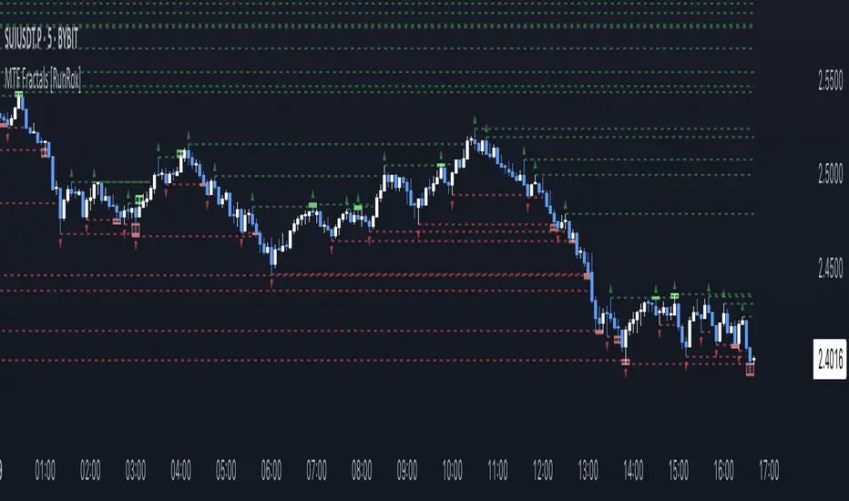
MTF Fractals [RunRox]🔽 MTF Fractals is a powerful indicator designed to visualize fractals from multiple timeframes directly on your chart, highlight liquidity sweeps at these fractal levels, and provide several additional features we’ll cover in detail below.
We created this indicator because we couldn’t find a suitable tool that met our specific needs on TradingView. Therefore, we decided to develop a valuable indicator for the entire TradingView community, combining simplicity and versatility.
⁉️ WHAT IS A FRACTALS?
In trading, a fractal is a technical analysis pattern composed of five consecutive candles, typically highlighting local market turning points. Specifically, a fractal high is formed when a candle’s high is higher than the highs of the two candles on either side, whereas a fractal low occurs when a candle’s low is lower than the lows of the two adjacent candles on both sides.
Traders use fractals as reference points for identifying significant support and resistance levels, potential reversal areas, and liquidity zones within price action analysis. Below is a screenshot illustrating clearly formed fractals on the chart.
📙 FRACTAL FORMATION
Here’s how fractals form depending on your chosen setting (3, 5, 7, or 9):
▶️ 3-bar fractal – forms when the central candle is higher (for highs) or lower (for lows) than one candle on each side.
▶️ 5-bar fractal – forms when the central candle is higher or lower than two candles on both sides.
▶️ 7-bar fractal – forms when the central candle is higher or lower compared to the three candles on each side.
▶️ 9-bar fractal – forms similarly but requires four candles on each side, making the fractal significantly more reliable and robust.
A higher number of bars ensures stronger fractal levels, highlighting more significant potential reversal points on the chart.
Now that we’ve covered the theory behind fractal formation, let’s explore the indicator’s functionality in more detail.
Below, I’ll explain each feature clearly and illustrate how you can effectively utilize this indicator in your trading.
🕐 MULTI-TIMEFRAME FRACTALS
We realized that displaying fractals only from the current timeframe isn’t always convenient, so we’ve introduced Multi-Timeframe Fractals into this indicator.
Now you can easily display fractals from higher timeframes directly on your current chart, providing you with broader market context and clearer trading signals.
Fractals from Current Timeframe – Fractals identified directly on the chart’s current timeframe.
Fractals from Higher Timeframes – Fractals sourced from higher timeframes and displayed clearly on your current chart for enhanced market perspective.
📈 FRACTAL LINES
Since fractals represent areas of high liquidity, we’ve added an option to extend fractal levels horizontally as Fractal Lines across your chart.
This feature allows you to clearly visualize critical liquidity areas from higher timeframes, directly on your current timeframe chart, as demonstrated in the screenshot below.
With this approach, you can clearly visualize significant fractal levels from higher timeframes directly on your current chart - for example, projecting fractals from the 1-hour (1H) timeframe onto a 3-minute (3m) chart. ✅ This helps you easily identify critical liquidity areas and potential reversal zones without the need to switch between multiple timeframes.
💰 LIQUDITY SWEEP (LIQUDITY GRAB)
To enhance your trading experience, we’ve introduced a feature that clearly identifies liquidity sweeps of fractal levels.
A Liquidity Sweep occurs when a candle closes beyond a fractal line, leaving a wick that pierces through it, signaling that liquidity has been collected at this level.
Below, you’ll find two examples illustrating this functionality:
▶️ Fractal lines from the current timeframe
▶️ Fractal lines projected from higher timeframes
The first example illustrates liquidity being swept from fractals on the current timeframe .
Here, the candle clearly closes beyond the fractal line, leaving a wick through it. This indicates a liquidity sweep at the fractal level, visually highlighting a potential reversal or continuation opportunity directly on your chart.
In the second example, fractals from the higher timeframe are projected onto your current chart.
When a candle on your current timeframe closes beyond an HTF fractal line - leaving a wick through this level - the indicator highlights it clearly. This signals to traders a potential reversal zone, indicating that liquidity has been swept, and price may reverse or significantly react from this area.
You can also enable the display of additional labels on the chart. These labels clearly mark liquidity sweeps at fractal levels, making it easier to visually identify potential reversal points directly on your chart.
⚙️ SETTINGS
Below are the indicator settings with detailed explanations for each parameter.
🔷 Bars in Fractal – Number of candles to the right and left required to form a fractal.
🔷 Fractal Timeframe – Select the timeframe from which you want to display fractals on the current chart.
🔷 Max Age, bars – Number of bars during which the fractal will remain active.
🔷 Show Fractal Line – Display or hide fractal lines.
🔷 Line Style – Choose the style of the line displayed on the chart.
🔷 Line Width – Thickness of the fractal line.
🔷 High Fractal – Style and color of bearish fractals.
🔷 Low Fractal – Style and color of bullish fractals.
🔷 Fractal Label Size – Select the size of fractal labels.
🔷 Show Sweep Labels – Option to display labels when a liquidity sweep occurs.
🔷 Label Color – Color and transparency of the area marked on the chart during a sweep.
🔷 Shade Sweep Area – Show or hide the sweep area shading.
🔷 Area Color – Color and transparency settings for the sweep area.
🔶 We’d love to hear your feedback and any suggestions for additional features you’d like to see in this indicator. We’ll be happy to consider your ideas and continue improving the indicator!
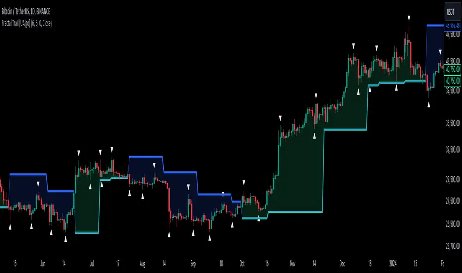
Fractal Trail [UAlgo]The Fractal Trail is designed to identify and utilize Williams fractals as dynamic trailing stops. This tool serves traders by marking key fractal points on the chart and leveraging them to create adaptive stop-loss trails, enhancing risk management and trade decision-making.
Williams fractals are pivotal in identifying potential reversals and critical support/resistance levels. By plotting fractals dynamically and providing configurable options, this indicator allows for personalized adjustments based on the trader's strategy.
This script integrates both visual fractal markers and adjustable trailing stops, offering insights into market trends while catering to a wide variety of trading styles and timeframes.
🔶 Key Features
Williams Fractals Identification: The indicator marks Williams Fractals on the chart, which are significant highs and lows within a specified range. These fractals are crucial for identifying potential reversal points in the market.
Dynamic Trailing Stops: The indicator generates dynamic trailing stops based on the identified fractals. These stops adjust automatically as new fractals are formed, providing a responsive and adaptive approach to risk management.
Fractal Range: Users can specify the number of bars to the left and right for analyzing fractals, allowing for flexibility in identifying significant price points.
Trail Buffer Percentage: A percentage-based safety margin can be added between the fractal price and the trailing stop, providing additional control over risk management.
Trail Invalidation Source: Users can choose whether the trailing stop flips based on candle closing prices or the extreme points (high/low) of the candles.
Alerts and Notifications: The indicator provides alerts for when the price crosses the trailing stops, as well as when new Williams Fractals are confirmed. These alerts can be customized to fit the trader's notification preferences.
🔶 Interpreting the Indicator
Fractal Markers: The triangles above and below the bars indicate Williams Fractals. These markers help traders identify potential reversal points in the market.
Trailing Stops: The dynamic trailing stops are plotted as lines on the chart. These lines adjust based on the latest identified fractals, providing a visual representation of potential support and resistance levels.
Fill Colors: The optional fill colors between the trailing stops and the price action help traders quickly identify the current trend and potential pullback zones.
🔶 Disclaimer
Use with Caution: This indicator is provided for educational and informational purposes only and should not be considered as financial advice. Users should exercise caution and perform their own analysis before making trading decisions based on the indicator's signals.
Not Financial Advice: The information provided by this indicator does not constitute financial advice, and the creator (UAlgo) shall not be held responsible for any trading losses incurred as a result of using this indicator.
Backtesting Recommended: Traders are encouraged to backtest the indicator thoroughly on historical data before using it in live trading to assess its performance and suitability for their trading strategies.
Risk Management: Trading involves inherent risks, and users should implement proper risk management strategies, including but not limited to stop-loss orders and position sizing, to mitigate potential losses.
No Guarantees: The accuracy and reliability of the indicator's signals cannot be guaranteed, as they are based on historical price data and past performance may not be indicative of future results.
Fractal Breakout Trend Following StrategyOverview
The Fractal Breakout Trend Following Strategy is a trend-following system which utilizes the Willams Fractals and Alligator to execute the long trades on the fractal's breakouts which have a high probability to be the new uptrend phase beginning. This system also uses the normalized Average True Range indicator to filter trades after a large moves, because it's more likely to see the trend continuation after a consolidation period. Strategy can execute only long trades.
Unique Features
Trend and volatility filtering system: Strategy uses Williams Alligator to filter the counter-trend fractals breakouts and normalized Average True Range to avoid the trades after large moves, when volatility is high
Configurable Trading Periods: Users can tailor the strategy to specific market windows, adapting to different market conditions.
Flexible Risk Management: Users can choose the stop-loss percent (by default = 3%) for trades, but strategy also has the dynamic stop-loss level using down fractals.
Methodology
The strategy places stop order at the last valid fractal breakout level. Validity of this fractal is defined by the Williams Alligator indicator. If at the moment of time when price breaking the last fractal price is higher than Alligator's teeth line (8 period SMA shifted 5 bars in the future) this is a valid breakout. Moreover strategy has the additional volatility filtering system using normalized ATR. It calculates the average normalized ATR for last user-defined number of bars and if this value lower than the user-defined threshold value the long trade is executed.
When trade is opened, script places the stop loss at the price higher of two levels: user defined stop-loss from the position entry price or down fractal validation level. The down fractal is valid with the rule, opposite as the up fractal validation. Price shall break to the downside the last down fractal below the Willians Alligator's teeth line.
Strategy has no fixed take profit. Exit level changes with the down fractal validation level. If price is in strong uptrend trade is going to be active until last down fractal is not valid. Strategy closes trade when price hits the down fractal validation level.
Risk Management
The strategy employs a combined approach to risk management:
It allows positions to ride the trend as long as the price continues to move favorably, aiming to capture significant price movements. It features a user-defined stop-loss parameter to mitigate risks based on individual risk tolerance. By default, this stop-loss is set to a 3% drop from the entry point, but it can be adjusted according to the trader's preferences.
Justification of Methodology
This strategy leverages Williams Fractals to open long trade when price has broken the key resistance level to the upside. This resistance level is the last up fractal and is shall be broken above the Williams Alligator's teeth line to be qualified as the valid breakout according to this strategy. The Alligator filtering increases the probability to avoid the false breakouts against the current trend.
Moreover strategy has an additional filter using Average True Range(ATR) indicator. If average value of ATR for the last user-defined number of bars is lower than user-defined threshold strategy can open the long trade according to open trade condition above. The logic here is following: we want to open trades after period of price consolidation inside the range because before and after a big move price is more likely to be in sideways, but we need a trend move to have a profit.
Another one important feature is how the exit condition is defined. On the one hand, strategy has the user-defined stop-loss (3% below the entry price by default). It's made to give users the opportunity to restrict their losses according to their risk-tolerance. On the other hand, strategy utilizes the dynamic exit level which is defined by down fractal activation. If we assume the breaking up fractal is the beginning of the uptrend, breaking down fractal can be the start of downtrend phase. We don't want to be in long trade if there is a high probability of reversal to the downside. This approach helps to not keep open trade if trend is not developing and hold it if price continues going up.
Backtest Results
Operating window: Date range of backtests is 2023.01.01 - 2024.05.01. It is chosen to let the strategy to close all opened positions.
Commission and Slippage: Includes a standard Binance commission of 0.1% and accounts for possible slippage over 5 ticks.
Initial capital: 10000 USDT
Percent of capital used in every trade: 30%
Maximum Single Position Loss: -3.19%
Maximum Single Profit: +24.97%
Net Profit: +3036.90 USDT (+30.37%)
Total Trades: 83 (28.92% win rate)
Profit Factor: 1.953
Maximum Accumulated Loss: 963.98 USDT (-8.29%)
Average Profit per Trade: 36.59 USDT (+1.12%)
Average Trade Duration: 72 hours
These results are obtained with realistic parameters representing trading conditions observed at major exchanges such as Binance and with realistic trading portfolio usage parameters.
How to Use
Add the script to favorites for easy access.
Apply to the desired timeframe and chart (optimal performance observed on 4h and higher time frames and the BTC/USDT).
Configure settings using the dropdown choice list in the built-in menu.
Set up alerts to automate strategy positions through web hook with the text: {{strategy.order.alert_message}}
Disclaimer:
Educational and informational tool reflecting Skyrex commitment to informed trading. Past performance does not guarantee future results. Test strategies in a simulated environment before live implementation

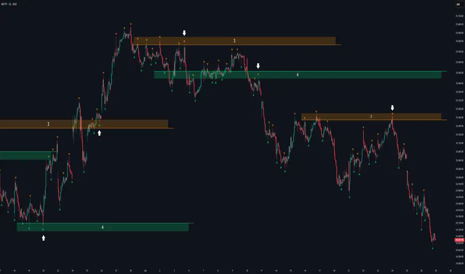
Fractal Support and Resistance [BigBeluga]🔵 OVERVIEW
The Fractal Support and Resistance indicator automatically identifies high-probability support and resistance zones based on repeated fractal touches. When a defined number of fractal highs or lows cluster around the same price zone, the indicator plots a clean horizontal level and shaded zone, helping traders visualize structurally important areas where price may react.
🔵 CONCEPTS
Fractal Points: Swing highs and lows based on user-defined left and right range (length). A valid fractal forms only when the center candle is higher or lower than its neighbors.
Zone Validation: A level is only confirmed when the price has printed the specified number of fractals (e.g., 3) within a narrow ATR-defined range.
Dynamic Zone Calculation: The plotted level can be based on the average of clustered fractals or on the extreme value (min or max), depending on the user’s choice.
Support/Resistance Zones: Once a zone is validated, a horizontal line and shaded box are drawn and automatically extended into the future until new valid clusters form.
Auto-Clean & Reactivity: Each zone persists until replaced by a new fractal cluster, ensuring the chart remains uncluttered and adaptive.
🔵 FEATURES
Detects swing fractals using adjustable left/right range.
Confirms zones when a defined number of fractals occur near the same price.
Plots horizontal level and shaded box for visual clarity.
Choice between average or min/max logic for level calculation.
Distinct color inputs for support (green) and resistance (orange) zones.
Adaptive auto-extension keeps valid zones projected into the future.
Displays optional triangle markers above/below bars where fractals form.
Clean design optimized for structural S/R analysis.
🔵 HOW TO USE
Use support zones (from low fractals) to look for potential long entries or bounce points .
Use resistance zones (from high fractals) to look for short setups or rejections .
Adjust the Fractals Qty to make zones more or less strict—e.g., 3 for higher reliability, 2 for quicker responsiveness.
Combine with liquidity indicators or break/retest logic to validate zone strength.
Toggle between average and min/max mode to fit your style (average for balance, extremes for aggression).
🔵 CONCLUSION
Fractal Support and Resistance offers a robust way to identify hidden levels that the market respects repeatedly. By requiring multiple fractal confirmations within a zone, it filters out noise and highlights clean structural areas of interest. This tool is ideal for traders who want automatic, adaptive, and reliable S/R levels grounded in raw market structure.
Fractals PivotsWhich trader does not know pivots? There are a lot of varieties of pivots indicators of which some are a default on most trading platforms. So what better way to challenge yourself then to create your own kind of pivots. Let's welcome the idea of Fractal Pivots.
Williams Fractal or fractals is a technical analysis indicator introduced by the famous trader Bill Williams in his book ‘Trading Chaos’. He developed it on the basis of the Chaos Theory and trading psychology. The indicator is centred around the idea that there is repetition in price behaviour and fractals can provide an insight into those repetitive patterns.
How does the indicator turn these into pivot lines?
The user will set a time period in which the script will look for fractals. It will then remember all the fractals that happen during that time period.
Let's say you are trading the hourly chart with a weekly pivot setting like in the chart this script is published on. The script will highling the 1h fractals that are happening. Then the next week it will use these exact fractals from previous week to draw the pivot lines.
Another example here is an 8h chart. Look how it uses the previous week fractals this week.
Let me know if you find a very great fractal length+timeframe setting where the levels really get respected. I would really appreciate that.

Evolution Fractals with IBA standard fractal high has two lower high (or equal high) candles to its left and right.
For standard fractal low fractals this is vice versa.
-But this indicator plots has the option to plot standard fractals only after candle close is confirmed.
So if the current candle is still forming in live markets, only after this candle has fully closed, then the indicator checks if the fractal is valid and then plotted.
You can select this option On or Off
(with the standard fractal indicator there is a fractal plotted, but when this candle high (or low ) is broken again, the fractal disappears. This re-painting of fractals can cause confusion.
-Added an alert functionality.
When setting an alert on your chart, you can select this indicator to alert you upon the forming of a new fractal high or low.
-Added optional Inside Bar function.
When a candle High/Low does not breach the previous candle High/Low, then a different body color can be shown.
This is particular handy to quickly if this high/low is breached, without having to zoom in on the chart.

Williams Fractals with BreaksThis is a Bill Williams fractal indicator with breaks.
I was turned onto fractals and the importance of their breaks by ChaosTrader63.
I know several version of this indicator have been done.
I chose this as a first project because of it's simplicity , but also because of the poor code quality of some other versions I looked at.
This is the first draft that successfully met my three criteria:
* Must identify all fractals, including simultaneous up/down fractals.
* Must identify fractal breaks with a clear indicator.
* Must provide information on how many fractals
For the first bullet, I wanted to provide a more concise modern version than the boolean logic composition I was seeing in other examples.
The later two required tracking the past which was not present in the other versions I looked at.
Code here can be improved for more uses and better integration, but it is functional and elegant enough to use.
Thanks for checking it out.
Jolly Wizard
Fractal Levels Monitor w/ Trade Lines (ChadAnt) v2Small update. Prevents the break candle from getting another signal after the first buy/sell signal detected.
1. Fractal Level Detection
The indicator identifies Fractals, which are simply a series of bars where the center bar has the highest high (Bearish Fractal) or the lowest low (Bullish Fractal) compared to a set number of bars on either side (determined by the "Fractal Period" input, usually 2 to 5 bars).
Bullish Fractal Level (Support): The indicator plots a horizontal line at the lowest low of the most recently formed Bullish Fractal.
Bearish Fractal Level (Resistance): It plots a horizontal line at the highest high of the most recently formed Bearish Fractal.
2. The "Cross Candle" Event
The core idea isn't to trade the fractal itself, but the reaction after the fractal level is broken.
When the price breaks and closes through the established Bullish Level (support) or Bearish Level (resistance), that bar is marked as the Cross Candle.
This Cross Candle's High and Low are saved. This is the "setup" for the trade.
3. The Trade Signal (Entry Trigger)
A trade is only taken when the price breaks the extreme (High or Low) of the Cross Candle.
Buy Signal: The trade is entered long if the price breaks above the High of the Cross Candle.
Sell Signal: The trade is entered short if the price breaks below the Low of the Cross Candle.

Fractal Levels Monitor w/ Trade Lines (ChadAnt)1. Fractal Level Detection
The indicator identifies Fractals, which are simply a series of bars where the center bar has the highest high (Bearish Fractal) or the lowest low (Bullish Fractal) compared to a set number of bars on either side (determined by the "Fractal Period" input, usually 2 to 5 bars).
Bullish Fractal Level (Support): The indicator plots a horizontal line at the lowest low of the most recently formed Bullish Fractal.
Bearish Fractal Level (Resistance): It plots a horizontal line at the highest high of the most recently formed Bearish Fractal.
2. The "Cross Candle" Event
The core idea isn't to trade the fractal itself, but the reaction after the fractal level is broken.
When the price breaks and closes through the established Bullish Level (support) or Bearish Level (resistance), that bar is marked as the Cross Candle.
This Cross Candle's High and Low are saved. This is the "setup" for the trade.
3. The Trade Signal (Entry Trigger)
A trade is only taken when the price breaks the extreme (High or Low) of the Cross Candle.
Buy Signal: The trade is entered long if the price breaks above the High of the Cross Candle.
Sell Signal: The trade is entered short if the price breaks below the Low of the Cross Candle.

(QUANTLABS) Fractal God Mode: 25-Timeframe Scanner The indicator aggregates data into three distinct metric columns:
1. STRUCT (Market Structure) This analyzes price action relative to Fractal Pivots (Highs and Lows) to determine market direction.
HH (Breakout): Price has closed above the previous Pivot High. (Bullish Structure)
LL (Breakdown): Price has closed below the previous Pivot Low. (Bearish Structure)
TRAPPED: Price is trading between the last Pivot High and Low. This indicates a ranging market where trend trades should be avoided.
2. VELOCITY (Thrust) This measures the specific strength of the current candle on that timeframe.
The Math: It calculates the ratio of the body (Close - Open) relative to the total candle range (High - Low).
The Signal: High positive numbers (Green) indicate buyers are closing near highs. High negative numbers (Red) indicate sellers are dominating the range.
3. QUALITY (Efficiency Ratio) This acts as a "Noise Filter." It determines if the trend is moving in a straight line or whipping back and forth.
The Math: It divides the Net Price Movement (Distance from 5 bars ago) by the Total Path Traveled (Sum of the ranges of the last 5 bars).
PRISTINE (Values > 0.6): The market is moving efficiently in one direction.
CHOPPY (Values < 0.4): The market is volatile and non-directional (High Noise).
1. The Matrix (Dashboard) Located in the bottom right, this table gives you an instant read on Short-Term (3m-9m), Medium-Term (10m-45m), and Long-Term (1H-Daily) trends.
2. Coherence Flow At the bottom of the table, the script sums up the structural score of all 25 timeframes.
COHERENT BULL: When the Short, Medium, and Long terms align green.
COHERENT BEAR: When the Short, Medium, and Long terms align red.
3. God Mode (Global S/R) The indicator can plot Support and Resistance levels from higher timeframes onto your current chart. For example, while trading the 5m chart, you can see the 4H and Daily pivot levels plotted automatically as dotted lines, ensuring you never trade blindly into a higher-timeframe wall.
Trend Following: Wait for the "Coherent Bull/Bear" signal at the bottom of the dashboard. This confirms that momentum is aligned from the 3m chart up to the Daily.
Scalping: Focus on the Quality column. Only take trades when the Quality is "CLEAN" or "PRISTINE." Avoid entries when the dashboard warns of "High Noise" (Choppy).
Risk Management: If the dashboard shows "TRAPPED" on the Long Term (1H+), reduce position size or wait for a breakout.
Pivot Lookback: Adjusts the sensitivity of the Fractal Structure (Default: 5).
Show Fractal DNA Matrix: Toggles the dashboard table.
Show ALL Timeframe S/R: Enables "God Mode" to see supports/resistances from all 25 timeframes (Heavy visual processing, use carefully).

[-_-] 2D FractalsThe sole purpose of this script is to demonstrate what's possible to make with Pinescript, namely to display images (2D Fractals in this case).
The script consists of two functions: one that generates the values of a fractal and one that displays them (utilising table) with each cell being used as a "pixel". We can control the "resolution" of image, as well as choose one of three fractal types.

Acc/Dist. Cloud with Fractal Deviation Bands by @XeL_ArjonaACCUMULATION / DISTRIBUTION CLOUD with MORPHIC DEVIATION BANDS
Ver. 2.0.beta.23:08:2015
by Ricardo M. Arjona @XeL_Arjona
DISCLAIMER
The Following indicator/code IS NOT intended to be a formal investment advice or recommendation by the author, nor should be construed as such. Users will be fully responsible by their use regarding their own trading vehicles/assets.
The embedded code and ideas within this work are FREELY AND PUBLICLY available on the Web for NON LUCRATIVE ACTIVITIES and must remain as is.
Pine Script code MOD's and adaptations by @XeL_Arjona with special mention in regard of:
Buy (Bull) and Sell (Bear) "Power Balance Algorithm by Vadim Gimelfarb published at Stocks & Commodities V. 21:10 (68-72).
Custom Weighting Coefficient for Exponential Moving Average (nEMA) adaptation work by @XeL_Arjona with contribution help from @RicardoSantos at TradingView @pinescript chat room.
Morphic Numbers (PHI & Plastic) Pine Script adaptation from it's algebraic generation formulas by @XeL_Arjona
Fractal Deviation Bands idea by @XeL_Arjona
CHANGE LOG:
ACCUMULATION / DISTRIBUTION CLOUD: I decided to change it's name from the Buy to Sell Pressure. The code is essentially the same as older versions and they are the center core (VORTEX?) of all derived New stuff which are:
MORPHIC NUMBERS: The "Golden Ratio" expressed by the result of the constant "PHI" and the newer and same in characteristics "Plastic Number" expressed as "PN". For more information about this regard take a look at: HERE!
CUSTOM(K) EXPONENTIAL MOVING AVERAGE: Some code has cleaned from last version to include as custom function the nEMA , which use an additional input (K) to customise the way the "exponentially" is weighted from the custom array. For the purpose of this indicator, I implement a volatility algorithm using the Average True Range of last 9 periods multiplied by the morphic number used in the fractal study. (Golden Ratio as default) The result is very similar in response to classic EMA but tend to accelerate or decelerate much more responsive with wider bars presented in trending average.
FRACTAL DEVIATION BANDS: The main idea is based on the so useful Standard Deviation process to create Bands in favor of a multiplier (As John Bollinger used in it's own bands) from a custom array, in which for this case is the "Volume Pressure Moving Average" as the main Vortex for the "Fractallitly", so then apply as many "Child bands" using the older one as the new calculation array using the same morphic constant as multiplier (Like Fibonacci but with other approach rather than %ratios). Results are AWSOME! Market tend to accelerate or decelerate their Trend in favor of a Fractal approach. This bands try to catch them, so please experiment and feedback me your own observations.
EXTERNAL TICKER FOR VOLUME DATA: I Added a way to input volume data for this kind of study from external tickers. This is just a quicky-hack given that currently TradingView is not adding Volume to their Indexes so; maybe this is temporary by now. It seems that this part of the code is conflicting with intraday timeframes, so You are advised.
This CODE is versioned as BETA FOR TESTING PROPOSES. By now TradingView Admins are changing lot's of things internally, so maybe this could conflict with correct rendering of this study with special tickers or timeframes. I will try to code by itself just the core parts of this study in order to use them at discretion in other areas. ALL NEW IDEAS OR MODIFICATIONS to these indicator(s) are Welcome in favor to deploy a better and more accurate readings. I will be very glad to be notified at Twitter or TradingView accounts at: @XeL_Arjona

Fractal Fade Pro IndicatorA revolutionary contrarian trading indicator that applies chaos theory, fractal mathematics, and market entropy to generate high-probability reverse signals. This indicator fades traditional technical signals, providing BUY signals when conventional indicators say SELL, and SELL signals when they say BUY.
Full Description:
Most traders follow the herd. QFCI does the opposite. It identifies when conventional technical analysis is about to fail by detecting mathematical patterns of exhaustion in market structure.
How It Works (Technical Overview):
The indicator combines three sophisticated mathematical approaches:
Fractal Dimension Analysis: Measures the "roughness" of price movements using fractal mathematics
Market Entropy Calculation: Quantifies the randomness and disorder in price returns using information theory
Phase Space Reconstruction: Analyzes price evolution in multi-dimensional state space from chaos theory
Signal Generation Process:
Step 1: Market Regime Detection
Chaotic Regime: High fractal complexity + rising entropy (avoid trading)
Trending Regime: Low fractal complexity + high phase space distance (fade breakouts)
Mean-Reverting Regime: Very low fractal complexity (fade extremes)
Step 2: Reverse Signal Logic
When traditional indicators would give:
BUY signal (breakout, oversold bounce, volatility spike) → QFCI shows SELL
SELL signal (breakdown, overbought rejection, volatility crash) → QFCI shows BUY
Step 3: Smart Signal Filtering
No consecutive same-direction signals
Adjustable minimum bars between signals
Multiple confirmation layers required
Unique Features:
1. Mathematical Innovation:
Original fractal dimension algorithm (not standard indicators)
Market entropy calculation from information theory
Phase space reconstruction from chaos theory
Multi-regime adaptive logic
2. Trading Psychology Advantage:
Contrarian by design - profits from market overreactions
Fades retail trader mistakes - enters when others are exiting
Reduces overtrading - strict signal frequency controls
3. Clean Visual Interface:
Only BUY/SELL labels - no chart clutter
Clear directional arrows - immediate signal recognition
Built-in alerts - never miss a trade
Recommended Settings:
Default (Balanced Approach):
Fractal Depth: 20
Entropy Period: 200
Min Bars Between Signals: 100
Aggressive Trading:
Fractal Depth: 10-15
Entropy Period: 100-150
Min Bars Between Signals: 50-75
Conservative Trading:
Fractal Depth: 30-40
Entropy Period: 300-400
Min Bars Between Signals: 150-200
Optimal Timeframes:
Primary: Daily, Weekly (best performance)
Secondary: 4-Hour, 12-Hour
Can work on: 1-Hour (with adjusted parameters)
How to Use:
For Beginners:
Apply indicator to chart
Use default settings
Wait for BUY/SELL labels
Enter on next candle open
Use 2:1 risk/reward ratio
Always use stop losses
For Advanced Traders:
Adjust parameters for your trading style
Combine with support/resistance levels
Use volume confirmation
Scale in/out of positions
Track performance by regime
Risk Management Guidelines:
Position Sizing:
Conservative: 1-2% risk per trade
Moderate: 2-3% risk per trade
Aggressive: 3-5% risk per trade (not recommended)
Stop Loss Placement:
BUY signals: Below recent swing low or -2x ATR
SELL signals: Above recent swing high or +2x ATR
Take Profit Targets:
Primary: 2x risk (minimum)
Secondary: Previous support/resistance
Tertiary: Trailing stops after 1.5x risk
IMPORTANT RISK DISCLOSURE
This indicator is for educational and informational purposes only. It is not financial advice. Past performance does not guarantee future results. Trading involves substantial risk of loss and is not suitable for every investor. The risk of loss in trading can be substantial. You should therefore carefully consider whether such trading is suitable for you in light of your financial condition.

Williams Fractals / Goldilocks [NPR21]📊 Williams Fractals — Goldilocks
Description
Williams Fractals — Goldilocks highlights confirmed swing highs and lows using a refined Williams Fractals approach that balances signal frequency and clarity. BUY and SELL labels mark structurally important pivot points while avoiding chart clutter. The Periods (n) setting controls how often signals appear—lower values produce more signals, higher values filter noise. Signals are non-repainting and work on any instrument and any timeframe. Best used as a market structure and confirmation tool.
🔧 How to Use (Quick Guide)
BUY labels = confirmed swing lows (potential support / pullback areas)
SELL labels = confirmed swing highs (potential resistance / exhaustion areas)
Use for structure and confirmation, not as a standalone entry system
Combine with trend direction, key levels, VWAP/EMAs, volume, or momentum
⏱️ Recommended Periods by Timeframe
The Periods (n) setting determines how many and how often labels print.
1m–3m (Scalping): n = 2
More frequent signals; captures short-term swings.
5m–15m (Intraday): n = 8-9
Balanced sensitivity; filters minor noise.
30m–1h+ (HTF/Swing): n = 15-21
Fewer, stronger pivots; highlights major structure.
Rule of thumb: Lower timeframe → lower n. Higher timeframe → higher n.
🌍 Markets & Timeframes
Not futures-only. Works well on stocks, ETFs, forex, crypto, indices, and any timeframe. Adjust n to match the market’s pace.

Adaptive Fractal Grid Scalping StrategyThis Pine Script v6 component implements an "Adaptive Fractal Grid Scalping Strategy" with an added volatility threshold feature.
Here's how it works:
Fractal Break Detection: Uses ta.pivothigh and ta.pivotlow to identify local highs and lows.
Volatility Clustering: Measures volatility using the Average True Range (ATR).
Adaptive Grid Levels: Dynamically adjusts grid levels based on ATR and user-defined multipliers.
Directional Bias Filter: Uses a Simple Moving Average (SMA) to determine trend direction.
Volatility Threshold: Introduces a new input to specify a minimum ATR value required to activate the strategy.
Trade Execution Logic: Places limit orders at grid levels based on trend direction and fractal levels, but only when ATR exceeds the volatility threshold.
Profit-Taking and Stop-Loss: Implements profit-taking at grid levels and a trailing stop-loss based on ATR.
How to Use
Inputs: Customize the ATR length, SMA length, grid multipliers, trailing stop multiplier, and volatility threshold through the input settings.
Visuals: The script plots fractal points and grid levels on the chart for easy visualization.
Trade Signals: The strategy automatically places buy/sell orders based on the detected fractals, trend direction, and volatility threshold.
Profit and Risk Management: The script includes logic for taking profits and setting stop-loss levels to manage trades effectively.
This strategy is designed to capitalize on micro-movements during high volatility and avoid overtrading during low-volatility trends. Adjust the input parameters to suit your trading style and market conditions.
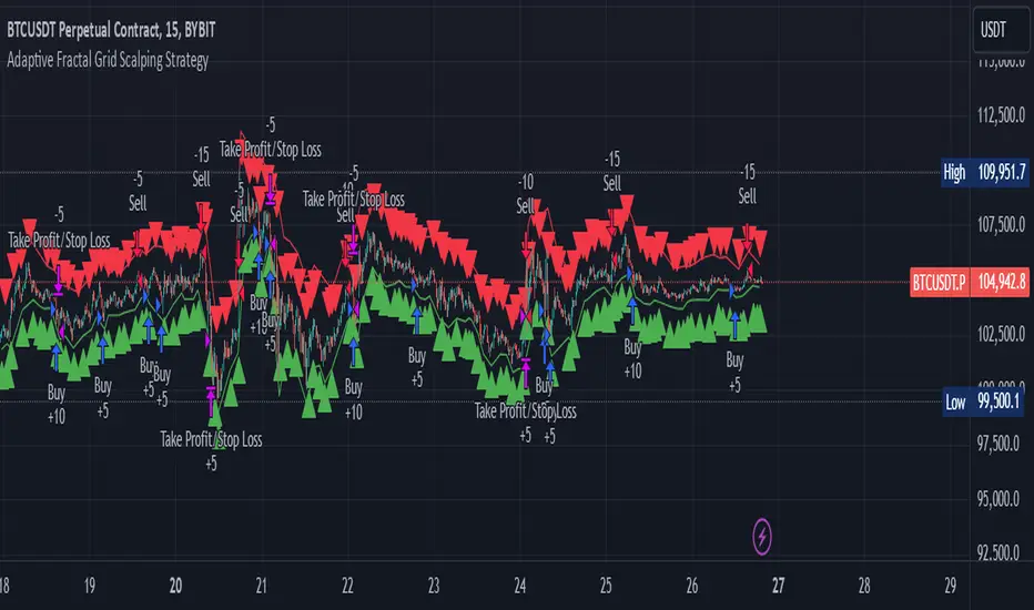
Fractal Proximity MA Aligment Scalping StrategyFractal Analysis
Fractals in trading help identify potential reversal points by marking significant price changes. Our strategy calculates a "fractal value" by comparing the current price to recent high and low fractal points. This is done by evaluating the sum of distances from the current closing price to the recent highs and lows. A positive fractal value suggests proximity to recent lows, hinting at upward momentum. Conversely, a negative value indicates closeness to recent highs, signaling potential downward movement.
Moving Averages for Confirmation
We use a series of 20 moving averages ranging from 5 to 100 to confirm trend directions indicated by fractal analysis. An entry signal is considered bullish when shorter-term moving averages are all above a long-term moving average, aligning with a positive fractal value.
Exit Strategy
The strategy employs dynamic stop-loss levels set at various moving averages, allowing for partial exits when the price crosses below specific thresholds. This helps manage the trade by locking in profits gradually. A full exit might be triggered by strong reversal signals suggested by both fractal values and moving average trends.
This open-source strategy is available for the community to test, adapt, and utilize. Your feedback and modifications are welcome as we refine the approach based on collective user experiences.

Correct Fractal Swings by CRYPTOFORThis indicator adjusts and enhances the normal 3-fractal swing. The author of this definition, uncle_travis, takes into account swings with the absorption of 3 candles and uses them as structure points.

Dynamic Fractal Flow [Alpha Extract]An advanced momentum oscillator that combines fractal market structure analysis with adaptive volatility weighting and multi-derivative calculus to identify high-probability trend reversals and continuation patterns. Utilizing sophisticated noise filtering through choppiness indexing and efficiency ratio analysis, this indicator delivers entries that adapt to changing market regimes while reducing false signals during consolidation via multi-layer confirmation centered on acceleration analysis, statistical band context, and dynamic omega weighting—without any divergence detection.
🔶 Fractal-Based Market Structure Detection
Employs Williams Fractal methodology to identify pivotal market highs and lows, calculating normalized price position within the established fractal range to generate oscillator signals based on structural positioning. The system tracks fractal points dynamically and computes relative positioning with ATR fallback protection, ensuring continuous signal generation even during extended trending periods without fractal formation.
🔶 Dynamic Omega Weighting System
Implements an adaptive weighting algorithm that adjusts signal emphasis based on real-time volatility conditions and volume strength, calculating dynamic omega coefficients ranging from 0.3 to 0.9. The system applies heavier weighting to recent price action during high-conviction moves while reducing sensitivity during low-volume environments, mitigating lag inherent in fixed-period calculations through volatility normalization and volume-strength integration.
🔶 Cascading Robustness Filtering
Features up to five stages of progressive EMA smoothing with user-adjustable robustness steps, each layer systematically filtering microstructure noise while preserving essential trend information. Smoothing periods scale with the chosen fractal length and robustness steps using a fixed smoothing multiplier for consistent, predictable behavior.
🔶 Adaptive Noise Suppression Engine
Integrates dual-component noise filtering combining Choppiness Index calculation with Kaufman’s Efficiency Ratio to detect ranging versus trending market conditions. The system applies dynamic damping that maintains full signal strength during trending environments while suppressing signals during choppy consolidation, aligning output with the prevailing regime.
🔶 Acceleration and Jerk Analysis Framework
Calculates second-derivative acceleration and third-derivative jerk to identify explosive momentum shifts before they fully materialize on traditional indicators. Detects bullish acceleration when both acceleration and jerk turn positive in negative oscillator territory, and bearish acceleration when both turn negative in positive territory, providing early entry signals for high-velocity trend initiation phases.
🔶 Multi-Layer Signal Generation Architecture
Combines three primary signal types with hierarchical validation: acceleration signals, band crossover entries, and threshold momentum signals. Each signal category includes momentum confirmation, trend-state validation, and statistical band context; signals are further conditioned by band squeeze detection to avoid low-probability entries during compression phases. Divergence is intentionally excluded for a purely structure- and momentum-driven approach.
🔶 Dynamic Statistical Band System
Utilizes Bollinger-style standard deviation bands with configurable multiplier and length to create adaptive threshold zones that expand during volatile periods and contract during consolidation. Includes band squeeze detection to identify compression phases that typically precede expansion, with signal suppression during squeezes to prevent premature entries.
🔶 Gradient Color Visualization System
Features color gradient mapping that dynamically adjusts line intensity based on signal strength, transitioning from neutral gray to progressively intense bullish or bearish colors as conviction increases. Includes gradient fills between the signal line and zero with transparency scaling based on oscillator intensity for immediate visual confirmation of trend strength and directional bias.
All analysis provided by Alpha Extract is for educational and informational purposes only. The information and publications are not meant to be, and do not constitute, financial, investment, trading, or other types of advice or recommendations.

FRPC - Fractal Reversal Permission ComponentThis tool identifies high-probability reversal points using a three-stage confirmation model:
1️⃣ Liquidity Sweep (LS)
Price must take out a previous fractal high/low, indicating stop-hunt liquidity removal.
2️⃣ Reclaim (RC)
After sweeping liquidity, price must close back inside the previous swing, showing absorption and rejection.
3️⃣ Break of Structure (BOS)
A structural break confirms a true shift in market direction and avoids false reversal signals.
FRPC only triggers BUY or SELL signals when all three layers align, creating actionable reversal conditions rather than random fractal noise.
This approach helps avoid chasing breakouts, filters low-quality sweeps, and identifies areas where reversals are statistically more likely.
------------------------------------
What FRRC Helps You Identify
------------------------------------
True reversals after stop-hunts
Liquidity grabs followed by displacement
Avoiding fake breakouts
Swing points with strong reaction potential
High-probability turning points with real structure support
----------
Sidenote
----------
The accuracy of the signals range from 56% to 72% and is mainly designed to be a structural filter to be paired with a strong exhaustion system. This is just a bare bones version and I plan to work on a more advanced version yo pair with the current exhaustion systems I'm building out

Overnight ES Strategy: CBC + Fractal + RSI + ATR FilterThis script is designed for overnight trading of the E-mini S&P 500 futures (ES) between 6 PM and 11 PM EST.
It combines multiple technical confluences to generate high-probability buy and sell signals, focusing on volatility-rich, low-liquidity evening sessions.
Key Features:
Candle Body Confluence (CBC) Approximation:
Identifies candles with small real bodies compared to total range, simulating consolidation zones where price is likely to reverse.
Williams Fractal Confirmation:
Detects local tops and bottoms based on 5-bar fractal reversal patterns, helping validate breakout or reversal points.
RSI Filter:
Ensures momentum is supportive — buys only when RSI < 35 (oversold) and sells only when RSI > 65 (overbought).
ATR Volatility Filter:
Trades are only allowed if the Average True Range (ATR) exceeds a user-defined threshold, filtering out low-volatility, risky environments.
Time Session Control:
Signals are only generated during the user-defined evening session (default: 6 PM to 11 PM EST) to match market behavior.
Real-Time Alerts Enabled:
Alerts can be set for BUY or SELL conditions, enabling mobile notifications, emails, or pop-ups without constant chart monitoring.
Recommended Settings:
Chart Timeframe: 15-minute or 30-minute candles
Assets: ES Mini (ES1!), NQ Mini, or other CME futures
Session: New York Time (EST)
ATR Threshold: Adjust based on market conditions; 5.0 suggested starting point for ES Mini on 15m.
Important:
This script only plots signals, it does not auto-execute trades.
Always backtest and paper trade before using live capital.
Volatility can vary; consider adjusting RSI and ATR filters based on market environment.
Credits:
Script designed based on confluence of price action, momentum, reversal structure, and volatility filtering principles used by professional traders.
Inspired by Candle Body Confluence (CBC) theory and Williams fractal techniques.