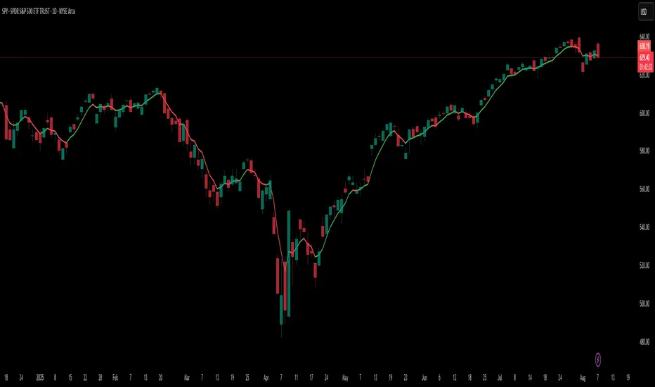
Dynamic 5DMA/EMA with Color for Multiple Products🔹 Dynamic 5DMA/EMA with Slope-Based Coloring (All Timeframes)
This indicator plots a dynamic 5-period moving average that adapts intelligently to your chart's timeframe and product type — giving you a clean, slope-sensitive visual edge across intraday, daily, and weekly views.
✅ Key Features:
📈 Dynamic MA Length Scaling:
On intraday timeframes, the MA adjusts for your selected market session (RTH, ETH, VIX, or Futures), calculating a true 5-day average based on actual session length — not just a flat bar count.
🔄 Automatic Timeframe Detection:
Daily Chart: Uses standard 5DMA or 5EMA.
Weekly Chart: Applies a true 5-week MA.
Intraday Charts: Converts 5 days into bar-length equivalent dynamically.
🎨 Color-Coded Slope Logic:
Green = Rising MA (bullish slope)
Red = Falling MA (bearish slope)
Neutral slope = previous color held for visual continuity
No more guessing — direction is instantly clear.
⚠️ Built-In Slope Flip Alerts:
Set alerts when the slope of the MA turns up or down. Ideal for timing pullback entries or exits across any product.
⚙️ Session Settings for Proper Scaling:
Choose your product's market structure to ensure accurate 5-day conversion on intraday charts:
Stocks - RTH: 390 mins/day
Stocks - ETH: 780 mins/day
VIX: 855 mins/day
Futures: 1440 mins/day
This ensures the MA reflects 5 full trading days, regardless of session irregularities or bar interval.
📌 Why Use This Indicator?
Most MAs misrepresent trend direction on intraday charts because they assume static daily bar counts. This tool corrects that, then adds slope-based coloring to give you a fast, visual read on short-term momentum. Whether you’re swing trading SPY, scalping VIX, or position trading futures, this indicator keeps your view aligned with how institutions see moving averages across timeframes.
🔧 Best For:
VIX & volatility traders
Short-term SPY/SPX traders
Swing traders who value clean setups
Anyone wanting a true 5-day trend anchor on any chart
Cerca negli script per "Futures"
Dskyz (DAFE) Aurora Divergence – Quant Master Dskyz (DAFE) Aurora Divergence – Quant Master
Introducing the Dskyz (DAFE) Aurora Divergence – Quant Master , a strategy that’s your secret weapon for mastering futures markets like MNQ, NQ, MES, and ES. Born from the legendary Aurora Divergence indicator, this fully automated system transforms raw divergence signals into a quant-grade trading machine, blending precision, risk management, and cyberpunk DAFE visuals that make your charts glow like a neon skyline. Crafted with care and driven by community passion, this strategy stands out in a sea of generic scripts, offering traders a unique edge to outsmart institutional traps and navigate volatile markets.
The Aurora Divergence indicator was a cult favorite for spotting price-OBV divergences with its aqua and fuchsia orbs, but traders craved a system to act on those signals with discipline and automation. This strategy delivers, layering advanced filters (z-score, ATR, multi-timeframe, session), dynamic risk controls (kill switches, adaptive stops/TPs), and a real-time dashboard to turn insights into profits. Whether you’re a newbie dipping into futures or a pro hunting reversals, this strat’s got your back with a beginner guide, alerts, and visuals that make trading feel like a sci-fi mission. Let’s dive into every detail and see why this original DAFE creation is a must-have.
Why Traders Need This Strategy
Futures markets are a battlefield—fast-paced, volatile, and riddled with institutional games that can wipe out undisciplined traders. From the April 28, 2025 NQ 1k-point drop to sneaky ES slippage, the stakes are high. Meanwhile, platforms are flooded with unoriginal, low-effort scripts that promise the moon but deliver noise. The Aurora Divergence – Quant Master rises above, offering:
Unmatched Originality: A bespoke system built from the ground up, with custom divergence logic, DAFE visuals, and quant filters that set it apart from copycat clutter.
Automation with Precision: Executes trades on divergence signals, eliminating emotional slip-ups and ensuring consistency, even in chaotic sessions.
Quant-Grade Filters: Z-score, ATR, multi-timeframe, and session checks filter out noise, targeting high-probability reversals.
Robust Risk Management: Daily loss and rolling drawdown kill switches, plus ATR-based stops/TPs, protect your capital like a fortress.
Stunning DAFE Visuals: Aqua/fuchsia orbs, aurora bands, and a glowing dashboard make signals intuitive and charts a work of art.
Community-Driven: Evolved from trader feedback, this strat’s a labor of love, not a recycled knockoff.
Traders need this because it’s a complete, original system that blends accessibility, sophistication, and style. It’s your edge to trade smarter, not harder, in a market full of traps and imitators.
1. Divergence Detection (Core Signal Logic)
The strategy’s core is its ability to detect bullish and bearish divergences between price and On-Balance Volume (OBV), pinpointing reversals with surgical accuracy.
How It Works:
Price Slope: Uses linear regression over a lookback (default: 9 bars) to measure price momentum (priceSlope).
OBV Slope: OBV tracks volume flow (+volume if price rises, -volume if falls), with its slope calculated similarly (obvSlope).
Bullish Divergence: Price slope negative (falling), OBV slope positive (rising), and price above 50-bar SMA (trend_ma).
Bearish Divergence: Price slope positive (rising), OBV slope negative (falling), and price below 50-bar SMA.
Smoothing: Requires two consecutive divergence bars (bullDiv2, bearDiv2) to confirm signals, reducing false positives.
Strength: Divergence intensity (divStrength = |priceSlope * obvSlope| * sensitivity) is normalized (0–1, divStrengthNorm) for visuals.
Why It’s Brilliant:
- Divergences catch hidden momentum shifts, often exploited by institutions, giving you an edge on reversals.
- The 50-bar SMA filter aligns signals with the broader trend, avoiding choppy markets.
- Adjustable lookback (min: 3) and sensitivity (default: 1.0) let you tune for different instruments or timeframes.
2. Filters for Precision
Four advanced filters ensure signals are high-probability and market-aligned, cutting through the noise of volatile futures.
Z-Score Filter:
Logic: Calculates z-score ((close - SMA) / stdev) over a lookback (default: 50 bars). Blocks entries if |z-score| > threshold (default: 1.5) unless disabled (useZFilter = false).
Impact: Avoids trades during extreme price moves (e.g., blow-off tops), keeping you in statistically safe zones.
ATR Percentile Volatility Filter:
Logic: Tracks 14-bar ATR in a 100-bar window (default). Requires current ATR > 80th percentile (percATR) to trade (tradeOk).
Impact: Ensures sufficient volatility for meaningful moves, filtering out low-volume chop.
Multi-Timeframe (HTF) Trend Filter:
Logic: Uses a 50-bar SMA on a higher timeframe (default: 60min). Longs require price > HTF MA (bullTrendOK), shorts < HTF MA (bearTrendOK).
Impact: Aligns trades with the bigger trend, reducing counter-trend losses.
US Session Filter:
Logic: Restricts trading to 9:30am–4:00pm ET (default: enabled, useSession = true) using America/New_York timezone.
Impact: Focuses on high-liquidity hours, avoiding overnight spreads and erratic moves.
Evolution:
- These filters create a robust signal pipeline, ensuring trades are timed for optimal conditions.
- Customizable inputs (e.g., zThreshold, atrPercentile) let traders adapt to their style without compromising quality.
3. Risk Management
The strategy’s risk controls are a masterclass in balancing aggression and safety, protecting capital in volatile markets.
Daily Loss Kill Switch:
Logic: Tracks daily loss (dayStartEquity - strategy.equity). Halts trading if loss ≥ $300 (default) and enabled (killSwitch = true, killSwitchActive).
Impact: Caps daily downside, crucial during events like April 27, 2025 ES slippage.
Rolling Drawdown Kill Switch:
Logic: Monitors drawdown (rollingPeak - strategy.equity) over 100 bars (default). Stops trading if > $1000 (rollingKill).
Impact: Prevents prolonged losing streaks, preserving capital for better setups.
Dynamic Stop-Loss and Take-Profit:
Logic: Stops = entry ± ATR * multiplier (default: 1.0x, stopDist). TPs = entry ± ATR * 1.5x (profitDist). Longs: stop below, TP above; shorts: vice versa.
Impact: Adapts to volatility, keeping stops tight but realistic, with TPs targeting 1.5:1 reward/risk.
Max Bars in Trade:
Logic: Closes trades after 8 bars (default) if not already exited.
Impact: Frees capital from stagnant trades, maintaining efficiency.
Kill Switch Buffer Dashboard:
Logic: Shows smallest buffer ($300 - daily loss or $1000 - rolling DD). Displays 0 (red) if kill switch active, else buffer (green).
Impact: Real-time risk visibility, letting traders adjust dynamically.
Why It’s Brilliant:
- Kill switches and ATR-based exits create a safety net, rare in generic scripts.
- Customizable risk inputs (maxDailyLoss, dynamicStopMult) suit different account sizes.
- Buffer metric empowers disciplined trading, a DAFE signature.
4. Trade Entry and Exit Logic
The entry/exit rules are precise, filtered, and adaptive, ensuring trades are deliberate and profitable.
Entry Conditions:
Long Entry: bullDiv2, cooldown passed (canSignal), ATR filter passed (tradeOk), in US session (inSession), no kill switches (not killSwitchActive, not rollingKill), z-score OK (zOk), HTF trend bullish (bullTrendOK), no existing long (lastDirection != 1, position_size <= 0). Closes shorts first.
Short Entry: Same, but for bearDiv2, bearTrendOK, no long (lastDirection != -1, position_size >= 0). Closes longs first.
Adaptive Cooldown: Default 2 bars (cooldownBars). Doubles (up to 10) after a losing trade, resets after wins (dynamicCooldown).
Exit Conditions:
Stop-Loss/Take-Profit: Set per trade (ATR-based). Exits on stop/TP hits.
Other Exits: Closes if maxBarsInTrade reached, ATR filter fails, or kill switch activates.
Position Management: Ensures no conflicting positions, closing opposites before new entries.
Built To Be Reliable and Consistent:
- Multi-filtered entries minimize false signals, a stark contrast to basic scripts.
- Adaptive cooldown prevents overtrading, especially after losses.
- Clean position handling ensures smooth execution, even in fast markets.
5. DAFE Visuals
The visuals are a DAFE hallmark, blending function with clean flair to make signals intuitive and charts stunning.
Aurora Bands:
Display: Bands around price during divergences (bullish: below low, bearish: above high), sized by ATR * bandwidth (default: 0.5).
Colors: Aqua (bullish), fuchsia (bearish), with transparency tied to divStrengthNorm.
Purpose: Highlights divergence zones with a glowing, futuristic vibe.
Divergence Orbs:
Display: Large/small circles (aqua below for bullish, fuchsia above for bearish) when bullDiv2/bearDiv2 and canSignal. Labels show strength (0–1).
Purpose: Pinpoints entries with eye-catching clarity.
Gradient Background:
Display: Green (bullish), red (bearish), or gray (neutral), 90–95% transparent.
Purpose: Sets the market mood without clutter.
Strategy Plots:
- Stop/TP Lines: Red (stops), green (TPs) for active trades.
- HTF MA: Yellow line for trend context.
- Z-Score: Blue step-line (if enabled).
- Kill Switch Warning: Red background flash when active.
What Makes This Next-Level?:
- Visuals make complex signals (divergences, filters) instantly clear, even for beginners.
- DAFE’s unique aesthetic (orbs, bands) sets it apart from generic scripts, reinforcing originality.
- Functional plots (stops, TPs) enhance trade management.
6. Metrics Dashboard
The top-right dashboard (2x8 table) is your command center, delivering real-time insights.
Metrics:
Daily Loss ($): Current loss vs. day’s start, red if > $300.
Rolling DD ($): Drawdown vs. 100-bar peak, red if > $1000.
ATR Threshold: Current percATR, green if ATR exceeds, red if not.
Z-Score: Current value, green if within threshold, red if not.
Signal: “Bullish Div” (aqua), “Bearish Div” (fuchsia), or “None” (gray).
Action: “Consider Buying”/“Consider Selling” (signal color) or “Wait” (gray).
Kill Switch Buffer ($): Smallest buffer to kill switch, green if > 0, red if 0.
Why This Is Important?:
- Consolidates critical data, making decisions effortless.
- Color-coded metrics guide beginners (e.g., green action = go).
- Buffer metric adds transparency, rare in off-the-shelf scripts.
7. Beginner Guide
Beginner Guide: Middle-right table (shown once on chart load), explains aqua orbs (bullish, buy) and fuchsia orbs (bearish, sell).
Key Features:
Futures-Optimized: Tailored for MNQ, NQ, MES, ES with point-value adjustments.
Highly Customizable: Inputs for lookback, sensitivity, filters, and risk settings.
Real-Time Insights: Dashboard and visuals update every bar.
Backtest-Ready: Fixed qty and tick calc for accurate historical testing.
User-Friendly: Guide, visuals, and dashboard make it accessible yet powerful.
Original Design: DAFE’s unique logic and visuals stand out from generic scripts.
How to Use
Add to Chart: Load on a 5min MNQ/ES chart in TradingView.
Configure Inputs: Adjust instrument, filters, or risk (defaults optimized for MNQ).
Monitor Dashboard: Watch signals, actions, and risk metrics (top-right).
Backtest: Run in strategy tester to evaluate performance.
Live Trade: Connect to a broker (e.g., Tradovate) for automation. Watch for slippage (e.g., April 27, 2025 ES issues).
Replay Test: Use bar replay (e.g., April 28, 2025 NQ drop) to test volatility handling.
Disclaimer
Trading futures involves significant risk of loss and is not suitable for all investors. Past performance is not indicative of future results. Backtest results may not reflect live trading due to slippage, fees, or market conditions. Use this strategy at your own risk, and consult a financial advisor before trading. Dskyz (DAFE) Trading Systems is not responsible for any losses incurred.
Backtesting:
Frame: 2023-09-20 - 2025-04-29
Fee Typical Range (per side, per contract)
CME Exchange $1.14 – $1.20
Clearing $0.10 – $0.30
NFA Regulatory $0.02
Firm/Broker Commis. $0.25 – $0.80 (retail prop)
TOTAL $1.60 – $2.30 per side
Round Turn: (enter+exit) = $3.20 – $4.60 per contract
Final Notes
The Dskyz (DAFE) Aurora Divergence – Quant Master isn’t just a strategy—it’s a movement. Crafted with originality and driven by community passion, it rises above the flood of generic scripts to deliver a system that’s as powerful as it is beautiful. With its quant-grade logic, DAFE visuals, and robust risk controls, it empowers traders to tackle futures with confidence and style. Join the DAFE crew, light up your charts, and let’s outsmart the markets together!
(This publishing will most likely be taken down do to some miscellaneous rule about properly displaying charting symbols, or whatever. Once I've identified what part of the publishing they want to pick on, I'll adjust and repost.)
Use it with discipline. Use it with clarity. Trade smarter.
**I will continue to release incredible strategies and indicators until I turn this into a brand or until someone offers me a contract.
Created by Dskyz, powered by DAFE Trading Systems. Trade fast, trade bold.

Adaptivity: Measures of Dominant Cycles and Price Trend [Loxx]Adaptivity: Measures of Dominant Cycles and Price Trend is an indicator that outputs adaptive lengths using various methods for dominant cycle and price trend timeframe adaptivity. While the information output from this indicator might be useful for the average trader in one off circumstances, this indicator is really meant for those need a quick comparison of dynamic length outputs who wish to fine turn algorithms and/or create adaptive indicators.
This indicator compares adaptive output lengths of all publicly known adaptive measures. Additional adaptive measures will be added as they are discovered and made public.
The first released of this indicator includes 6 measures. An additional three measures will be added with updates. Please check back regularly for new measures.
Ehers:
Autocorrelation Periodogram
Band-pass
Instantaneous Cycle
Hilbert Transformer
Dual Differentiator
Phase Accumulation (future release)
Homodyne (future release)
Jurik:
Composite Fractal Behavior (CFB)
Adam White:
Veritical Horizontal Filter (VHF) (future release)
What is an adaptive cycle, and what is Ehlers Autocorrelation Periodogram Algorithm?
From his Ehlers' book Cycle Analytics for Traders Advanced Technical Trading Concepts by John F. Ehlers , 2013, page 135:
"Adaptive filters can have several different meanings. For example, Perry Kaufman's adaptive moving average (KAMA) and Tushar Chande's variable index dynamic average (VIDYA) adapt to changes in volatility . By definition, these filters are reactive to price changes, and therefore they close the barn door after the horse is gone.The adaptive filters discussed in this chapter are the familiar Stochastic , relative strength index (RSI), commodity channel index (CCI), and band-pass filter.The key parameter in each case is the look-back period used to calculate the indicator. This look-back period is commonly a fixed value. However, since the measured cycle period is changing, it makes sense to adapt these indicators to the measured cycle period. When tradable market cycles are observed, they tend to persist for a short while.Therefore, by tuning the indicators to the measure cycle period they are optimized for current conditions and can even have predictive characteristics.
The dominant cycle period is measured using the Autocorrelation Periodogram Algorithm. That dominant cycle dynamically sets the look-back period for the indicators. I employ my own streamlined computation for the indicators that provide smoother and easier to interpret outputs than traditional methods. Further, the indicator codes have been modified to remove the effects of spectral dilation.This basically creates a whole new set of indicators for your trading arsenal."
What is this Hilbert Transformer?
An analytic signal allows for time-variable parameters and is a generalization of the phasor concept, which is restricted to time-invariant amplitude, phase, and frequency. The analytic representation of a real-valued function or signal facilitates many mathematical manipulations of the signal. For example, computing the phase of a signal or the power in the wave is much simpler using analytic signals.
The Hilbert transformer is the technique to create an analytic signal from a real one. The conventional Hilbert transformer is theoretically an infinite-length FIR filter. Even when the filter length is truncated to a useful but finite length, the induced lag is far too large to make the transformer useful for trading.
From his Ehlers' book Cycle Analytics for Traders Advanced Technical Trading Concepts by John F. Ehlers , 2013, pages 186-187:
"I want to emphasize that the only reason for including this section is for completeness. Unless you are interested in research, I suggest you skip this section entirely. To further emphasize my point, do not use the code for trading. A vastly superior approach to compute the dominant cycle in the price data is the autocorrelation periodogram. The code is included because the reader may be able to capitalize on the algorithms in a way that I do not see. All the algorithms encapsulated in the code operate reasonably well on theoretical waveforms that have no noise component. My conjecture at this time is that the sample-to-sample noise simply swamps the computation of the rate change of phase, and therefore the resulting calculations to find the dominant cycle are basically worthless.The imaginary component of the Hilbert transformer cannot be smoothed as was done in the Hilbert transformer indicator because the smoothing destroys the orthogonality of the imaginary component."
What is the Dual Differentiator, a subset of Hilbert Transformer?
From his Ehlers' book Cycle Analytics for Traders Advanced Technical Trading Concepts by John F. Ehlers , 2013, page 187:
"The first algorithm to compute the dominant cycle is called the dual differentiator. In this case, the phase angle is computed from the analytic signal as the arctangent of the ratio of the imaginary component to the real component. Further, the angular frequency is defined as the rate change of phase. We can use these facts to derive the cycle period."
What is the Phase Accumulation, a subset of Hilbert Transformer?
From his Ehlers' book Cycle Analytics for Traders Advanced Technical Trading Concepts by John F. Ehlers , 2013, page 189:
"The next algorithm to compute the dominant cycle is the phase accumulation method. The phase accumulation method of computing the dominant cycle is perhaps the easiest to comprehend. In this technique, we measure the phase at each sample by taking the arctangent of the ratio of the quadrature component to the in-phase component. A delta phase is generated by taking the difference of the phase between successive samples. At each sample we can then look backwards, adding up the delta phases.When the sum of the delta phases reaches 360 degrees, we must have passed through one full cycle, on average.The process is repeated for each new sample.
The phase accumulation method of cycle measurement always uses one full cycle's worth of historical data.This is both an advantage and a disadvantage.The advantage is the lag in obtaining the answer scales directly with the cycle period.That is, the measurement of a short cycle period has less lag than the measurement of a longer cycle period. However, the number of samples used in making the measurement means the averaging period is variable with cycle period. longer averaging reduces the noise level compared to the signal.Therefore, shorter cycle periods necessarily have a higher out- put signal-to-noise ratio."
What is the Homodyne, a subset of Hilbert Transformer?
From his Ehlers' book Cycle Analytics for Traders Advanced Technical Trading Concepts by John F. Ehlers , 2013, page 192:
"The third algorithm for computing the dominant cycle is the homodyne approach. Homodyne means the signal is multiplied by itself. More precisely, we want to multiply the signal of the current bar with the complex value of the signal one bar ago. The complex conjugate is, by definition, a complex number whose sign of the imaginary component has been reversed."
What is the Instantaneous Cycle?
The Instantaneous Cycle Period Measurement was authored by John Ehlers; it is built upon his Hilbert Transform Indicator.
From his Ehlers' book Cybernetic Analysis for Stocks and Futures: Cutting-Edge DSP Technology to Improve Your Trading by John F. Ehlers, 2004, page 107:
"It is obvious that cycles exist in the market. They can be found on any chart by the most casual observer. What is not so clear is how to identify those cycles in real time and how to take advantage of their existence. When Welles Wilder first introduced the relative strength index (rsi), I was curious as to why he selected 14 bars as the basis of his calculations. I reasoned that if i knew the correct market conditions, then i could make indicators such as the rsi adaptive to those conditions. Cycles were the answer. I knew cycles could be measured. Once i had the cyclic measurement, a host of automatically adaptive indicators could follow.
Measurement of market cycles is not easy. The signal-to-noise ratio is often very low, making measurement difficult even using a good measurement technique. Additionally, the measurements theoretically involve simultaneously solving a triple infinity of parameter values. The parameters required for the general solutions were frequency, amplitude, and phase. Some standard engineering tools, like fast fourier transforms (ffs), are simply not appropriate for measuring market cycles because ffts cannot simultaneously meet the stationarity constraints and produce results with reasonable resolution. Therefore i introduced maximum entropy spectral analysis (mesa) for the measurement of market cycles. This approach, originally developed to interpret seismographic information for oil exploration, produces high-resolution outputs with an exceptionally short amount of information. A short data length improves the probability of having nearly stationary data. Stationary data means that frequency and amplitude are constant over the length of the data. I noticed over the years that the cycles were ephemeral. Their periods would be continuously increasing and decreasing. Their amplitudes also were changing, giving variable signal-to-noise ratio conditions. Although all this is going on with the cyclic components, the enduring characteristic is that generally only one tradable cycle at a time is present for the data set being used. I prefer the term dominant cycle to denote that one component. The assumption that there is only one cycle in the data collapses the difficulty of the measurement process dramatically."
What is the Band-pass Cycle?
From his Ehlers' book Cycle Analytics for Traders Advanced Technical Trading Concepts by John F. Ehlers , 2013, page 47:
"Perhaps the least appreciated and most underutilized filter in technical analysis is the band-pass filter. The band-pass filter simultaneously diminishes the amplitude at low frequencies, qualifying it as a detrender, and diminishes the amplitude at high frequencies, qualifying it as a data smoother. It passes only those frequency components from input to output in which the trader is interested. The filtering produced by a band-pass filter is superior because the rejection in the stop bands is related to its bandwidth. The degree of rejection of undesired frequency components is called selectivity. The band-stop filter is the dual of the band-pass filter. It rejects a band of frequency components as a notch at the output and passes all other frequency components virtually unattenuated. Since the bandwidth of the deep rejection in the notch is relatively narrow and since the spectrum of market cycles is relatively broad due to systemic noise, the band-stop filter has little application in trading."
From his Ehlers' book Cycle Analytics for Traders Advanced Technical Trading Concepts by John F. Ehlers , 2013, page 59:
"The band-pass filter can be used as a relatively simple measurement of the dominant cycle. A cycle is complete when the waveform crosses zero two times from the last zero crossing. Therefore, each successive zero crossing of the indicator marks a half cycle period. We can establish the dominant cycle period as twice the spacing between successive zero crossings."
What is Composite Fractal Behavior (CFB)?
All around you mechanisms adjust themselves to their environment. From simple thermostats that react to air temperature to computer chips in modern cars that respond to changes in engine temperature, r.p.m.'s, torque, and throttle position. It was only a matter of time before fast desktop computers applied the mathematics of self-adjustment to systems that trade the financial markets.
Unlike basic systems with fixed formulas, an adaptive system adjusts its own equations. For example, start with a basic channel breakout system that uses the highest closing price of the last N bars as a threshold for detecting breakouts on the up side. An adaptive and improved version of this system would adjust N according to market conditions, such as momentum, price volatility or acceleration.
Since many systems are based directly or indirectly on cycles, another useful measure of market condition is the periodic length of a price chart's dominant cycle, (DC), that cycle with the greatest influence on price action.
The utility of this new DC measure was noted by author Murray Ruggiero in the January '96 issue of Futures Magazine. In it. Mr. Ruggiero used it to adaptive adjust the value of N in a channel breakout system. He then simulated trading 15 years of D-Mark futures in order to compare its performance to a similar system that had a fixed optimal value of N. The adaptive version produced 20% more profit!
This DC index utilized the popular MESA algorithm (a formulation by John Ehlers adapted from Burg's maximum entropy algorithm, MEM). Unfortunately, the DC approach is problematic when the market has no real dominant cycle momentum, because the mathematics will produce a value whether or not one actually exists! Therefore, we developed a proprietary indicator that does not presuppose the presence of market cycles. It's called CFB (Composite Fractal Behavior) and it works well whether or not the market is cyclic.
CFB examines price action for a particular fractal pattern, categorizes them by size, and then outputs a composite fractal size index. This index is smooth, timely and accurate
Essentially, CFB reveals the length of the market's trending action time frame. Long trending activity produces a large CFB index and short choppy action produces a small index value. Investors have found many applications for CFB which involve scaling other existing technical indicators adaptively, on a bar-to-bar basis.
What is VHF Adaptive Cycle?
Vertical Horizontal Filter (VHF) was created by Adam White to identify trending and ranging markets. VHF measures the level of trend activity, similar to ADX DI. Vertical Horizontal Filter does not, itself, generate trading signals, but determines whether signals are taken from trend or momentum indicators. Using this trend information, one is then able to derive an average cycle length.

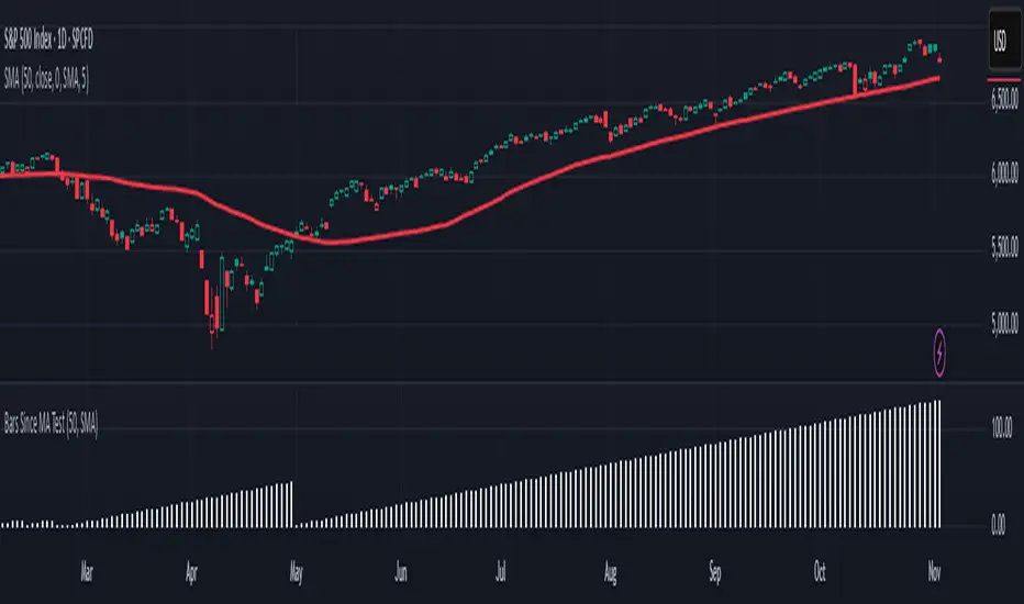
Is it Time for a Pullback? Check Bars Since MA TestAn old market adage declares that “prices never move in a straight line.” Dips occur even in bullish markets. But how can traders know when prices may be due for a pullback?
Today’s script tries to answer that question by asking how many bars have passed since a stock, index or other symbol has tested a given moving average. Long periods of time without touching a line such as the 50-day simple moving average, for example, could prompt traders to be more patient.
Bars Since MA Test counts how many bars have passed since prices touched or crossed the MA in question. The resulting value is plotted in a simple histogram. Users can set the MA length and type. By default, it uses the 50-day simple moving average (SMA).
The chart above applies Bars Since MA Test to the S&P 500. It shows that the index has gone 129 bars without testing its 50-day SMA. That’s the longest since a 146-bar stretch between July 2006 and February 2007.
Other longer runs include January-August 1995 (156 bars), November 1960-June 1961 (144 bars) and April-November 1958 (158 bars).
Given the small number of comparable readings, could traders suspect the current advance is getting long in the tooth?
TradeStation has, for decades, advanced the trading industry, providing access to stocks, options and futures. If you're born to trade, we could be for you. See our Overview for more.
Past performance, whether actual or indicated by historical tests of strategies, is no guarantee of future performance or success. There is a possibility that you may sustain a loss equal to or greater than your entire investment regardless of which asset class you trade (equities, options or futures); therefore, you should not invest or risk money that you cannot afford to lose. Online trading is not suitable for all investors. View the document titled Characteristics and Risks of Standardized Options at www.TradeStation.com . Before trading any asset class, customers must read the relevant risk disclosure statements on www.TradeStation.com . System access and trade placement and execution may be delayed or fail due to market volatility and volume, quote delays, system and software errors, Internet traffic, outages and other factors.
Securities and futures trading is offered to self-directed customers by TradeStation Securities, Inc., a broker-dealer registered with the Securities and Exchange Commission and a futures commission merchant licensed with the Commodity Futures Trading Commission). TradeStation Securities is a member of the Financial Industry Regulatory Authority, the National Futures Association, and a number of exchanges.
TradeStation Securities, Inc. and TradeStation Technologies, Inc. are each wholly owned subsidiaries of TradeStation Group, Inc., both operating, and providing products and services, under the TradeStation brand and trademark. When applying for, or purchasing, accounts, subscriptions, products and services, it is important that you know which company you will be dealing with. Visit www.TradeStation.com for further important information explaining what this means.
Breakdown or Buyable Dip? Pullback Depth Can HelpAs a common adage says, “the market doesn’t move in a straight line.” But when prices have fallen, it’s not always clear whether buying makes sense. That’s where today’s script may help.
Most traditional indicators judge movement based on price. That’s obviously important, but time can also be helpful. After all, there’s a big difference between probing a low from 2-3 weeks ago versus a low from months or even years in the past.
Pullback Depth clearly illustrates this by answering the question: “Today’s low is the lowest in how many bars?”
The resulting integer is plotted in a simple histogram. Values are always negative because bars with higher absolute values (meaning more negative, or further below zero) are potentially more bearish.
The study also has a maximum lookback period to avoid overwhelming the study with too many bars. Its default setting of 125 bars includes enough history to illustrate the trend.
The stock market’s recent run has seen only shallow pullbacks. Most dips have probed 1-2 weeks in the past, while Friday’s selloff only turned back the clock a month.
Consider two other previous moments.
First, the great bull run of 1995 saw only shallow pullbacks. (None exceeded 50 days.):
In contrast, early 2022 saw the S&P 500 test levels more than 100 candles into the past. It soon fell into an official “bear market:”
TradeStation has, for decades, advanced the trading industry, providing access to stocks, options and futures. If you're born to trade, we could be for you. See our Overview for more.
Past performance, whether actual or indicated by historical tests of strategies, is no guarantee of future performance or success. There is a possibility that you may sustain a loss equal to or greater than your entire investment regardless of which asset class you trade (equities, options or futures); therefore, you should not invest or risk money that you cannot afford to lose. Online trading is not suitable for all investors. View the document titled Characteristics and Risks of Standardized Options at www.TradeStation.com . Before trading any asset class, customers must read the relevant risk disclosure statements on www.TradeStation.com . System access and trade placement and execution may be delayed or fail due to market volatility and volume, quote delays, system and software errors, Internet traffic, outages and other factors.
Securities and futures trading is offered to self-directed customers by TradeStation Securities, Inc., a broker-dealer registered with the Securities and Exchange Commission and a futures commission merchant licensed with the Commodity Futures Trading Commission). TradeStation Securities is a member of the Financial Industry Regulatory Authority, the National Futures Association, and a number of exchanges.
TradeStation Securities, Inc. and TradeStation Technologies, Inc. are each wholly owned subsidiaries of TradeStation Group, Inc., both operating, and providing products and services, under the TradeStation brand and trademark. When applying for, or purchasing, accounts, subscriptions, products and services, it is important that you know which company you will be dealing with. Visit www.TradeStation.com for further important information explaining what this means.

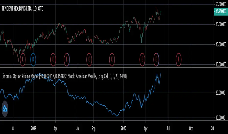
Binomial Option Pricing ModelA binomial option pricing model is an option pricing model that calculates an option's price using binomial trees. The BOPM method of calculating option prices is different from the Black-Scholes Model because it provides more flexibility in the type of options you want to price. The BOPM, unlike the BS model typically used for European style options, allows you to price options which have the ability to exercise early, such as American or Bermudan options. Although you can use the BOPM for any option style.
This specific model allows you to price both American and European vanilla options.
The way the BOPM calculates option prices is by:
First, dividing up the time until expiry into equal parts called steps. This specific model presented only uses 2 steps. For example, say you have an option with an expiry of 60 days, and your binomial tree has only two steps. Then each step will contain 30 days.
Second, the model will project the expected price of the underlying at the end of each step, called a node. The expected price is calculated by using the underlying's volatility and projecting what the price of the underlying would be if it were to rise and fall. This step is repeated until the terminal node, aka the end of the tree, is reached.
Third, once the terminal node's expected underlying prices are calculated, their expected option prices must be calculated.
Finally, after calculating the terminal option prices, backwards induction must be used to calculate the option prices at the previous nodes, until you reach Node 0, aka the current option price.
In order to use this model:
1st. Enter your option's strike price.
2nd. Enter the risk-free-rate of the currency the option is based in.
3rd. Enter the dividend yield of the underlying if it's a stock, or the foreign risk-free-rate if it's an FX option.
*For example, if you were trading an AAPL stock option, in the risk-free-rate box mentioned in step 2, you would enter the US risk-free-rate because AAPL options are traded in US dollars. In the dividend yield box mentioned in step 3, you would enter the stock's dividend yield, which for AAPL is 0.82.
*If you were, for example, trading an option on the EUR/JPY currency pair, the risk-free-rate mentioned in step 2, would be the Japanese risk-free-rate. Then in the the dividend yield box from step 3, you'd input the Eurozone risk-free-rate.
*If you were trading an options on futures contract, the risk-free-rate mentioned in step 2, would be the risk-free-rate for whatever currency the futures contract is denominated in. For example EUR futures are denominated in USD, so you would input the US risk-free-rate. Meanwhile, something like FTSE futures are denominated in GBP, so you would input the British risk-free-rate. As for the dividend yield box mentioned in step 3, for all options on futures, enter 0.
4th. Pick what type of underlying the option is based on: stock, FX, or futures.
5th. Pick the style of option: American or European.
6th. Pick the type of option: Long Call or Long Put.
7th. Input your time until expiry. You can express this in terms of days, hours, and minutes.
8th. Lastly, input your chart time-frame in term of minutes. For example, if you're using the 1 min time-frame enter 1, 4hr time-frame enter 480, daily time-frame enter 1440.
*Disclaimer, because this particular model only uses 2 steps, it won't work on stocks with high prices (over $100). If you want to use this on stocks with prices greater than $100, you would need to add more steps to the code, shown below. The model in its current form should work for stocks below $100.
cephxs / New X Opening Gaps [Pro +]NWOG & NDOG - OPENING GAPS
Smart Gap Detection with Intelligent Filtering
Visualizes New Week Opening Gaps (NWOGs) and New Day Opening Gaps (NDOGs) with built-in intelligence to show you only what matters. No more cluttered charts with gaps from 3 months ago that price will never revisit.
THE PROBLEM WITH GAP INDICATORS
Most gap indicators dump every single gap on your chart and call it a day. You end up with 50 boxes cluttering your screen, half of which are miles away from current price and the other half are so tiny they're basically noise.
This one's different and I explain why below.
SMART FILTERING (THE GOOD STUFF)
Two filters work together to keep your chart clean:
Size Filter: Uses ATR-based detection to filter out insignificant gaps, dynamic with less volatile time periods
- Filter None: Show everything (if you really want chaos)
- Filter Insignificant: Hide the micro-gaps that don't matter
- Juicy Gaps Only: Only show gaps worth paying attention to
Distance Filter: Only displays gaps within range of current price
- Really Close: 0.5 ATR - tight focus on immediate levels
- Balanced: 1 ATR - sweet spot for most traders
- Slightly Far: 3 ATR - wider view for swing traders
Cleanup Interval: Controls how quickly out-of-range gaps disappear
- Immediately: Gaps hide/show every bar as price moves
- 5 / 15 / 30 Minutes: Gaps only update visibility at interval boundaries - reduces visual noise during choppy price action
The magic: gaps appear and disappear as price moves toward or away from them. Old gaps that price has left behind fade out, and gaps that become relevant fade back in. Use delayed cleanup intervals if you want gaps to "stick around" a bit longer before disappearing.
GAP TYPES EXPLAINED
New Week Opening Gaps (NWOGs):
The gap between Friday's close and Monday's open. These form over the weekend when markets are closed and often act as significant support/resistance.
Two classifications:
Void Gaps: Gap direction aligns with Friday's candle direction (continuation)
Overlap Gaps: Gap direction conflicts with Friday's candle (potential reversal)
New Day Opening Gaps (NDOGs):
The gap between one day's close and the next day's open. Smaller but frequent - useful for intraday traders looking for fill targets.
FEATURES
Automatic Week/Day Detection: Handles forex (17:00 ET open) and futures (18:00 ET open) correctly
DST-Aware: Uses New York timezone with automatic daylight saving adjustments
50% Equilibrium Line: Marks the midpoint of each gap - key level for entries
Days Ago Labels: Shows how old each gap is at a glance
Extension Modes: Choose between live-extending boxes or fixed-width boxes
Separate Color Schemes: Different colors for void vs overlap NWOGs, bullish vs bearish NDOGs
INPUTS
NWOG Display
Show NWOGs: Master toggle
Extension Mode: "Extend Live" or "Extend to Week Close"
Maximum NWOGs: Limit displayed gaps (1-50)
Show Void/Overlap Gaps: Toggle each type independently
Show NWOG Labels: Toggle gap labels
NDOG Display
Show NDOGs: Master toggle
Extension Mode: "Extend Live" or "Extend to Day Close"
Maximum NDOGs: Limit displayed gaps (1-50)
Show NDOG Labels: Toggle gap labels
Filter Settings
Size Filter: Filter None / Filter Insignificant / Juicy Gaps Only
Only Show Near Price: Enable/disable distance filtering
Distance Filter: Really Close / Balanced / Slightly Far
Cleanup Interval: Immediately / 5 Minutes / 15 Minutes / 30 Minutes - controls how often gaps update visibility
ATR Period: Period for ATR calculation (default: 14)
Right Edge Offset: How many bars ahead boxes extend
Styling
Box Transparency: Fill and border opacity
Midline Style: Solid / Dotted / Dashed
Label Style: Simple ("NWOG, 5d ago") or Descriptive ("NWOG (Void Bull), 5d ago")
Label Size: Tiny / Small / Normal / Large
RECOMMENDED SETTINGS
For intraday (1m-15m):
Size Filter: Filter Insignificant
Distance Filter: Really Close or Balanced
Show NDOGs: On
Maximum NDOGs: 5-10
For swing trading (1H-4H):
Size Filter: Juicy Gaps Only
Distance Filter: Balanced or Slightly Far
Show NWOGs: On
Maximum NWOGs: 10-20
TIMEFRAME NOTES
Works on daily timeframe and below. Above daily, the indicator disables itself since NWOG/NDOG gap detection requires daily open/close data.
ASSET SUPPORT
Automatically handles different market open times:
Forex: Week opens Sunday 17:00 ET, closes Friday 17:00 ET
Futures: Week opens Sunday 18:00 ET, closes Friday 16:15 ET
Stocks/Other: Uses session-based detection
FAQ
Why do gaps appear and disappear?
That's the distance filter working. As price moves, gaps that were far away become relevant and appear. Gaps that price leaves behind disappear. This keeps your chart focused on actionable levels.
What's the difference between void and overlap gaps?
Void gaps continue Friday's direction (trend continuation). Overlap gaps conflict with Friday's direction (potential reversal setup). Different traders prefer different types.
Why can't I see any gaps?
Check your filter settings. "Juicy Gaps Only" with "Really Close" distance filter is very selective. Try "Filter Insignificant" with "Balanced" for more gaps.
DISCLAIMER
This indicator is for educational purposes only. Opening gaps are one tool among many - they don't guarantee fills or reversals. Always use proper risk management and never trade based on a single indicator. Past gap fills don't guarantee future performance. Do your own analysis.
CHANGELOG
Pro +: Added smart size/distance filtering, void/overlap classification, NDOG support, DST-aware timezone handling
Base: Initial NWOG visualization
Made with ❤️ by fstarlabs

HA Trend Reclaim Daily Structure Pullback🔹 HA Trend Reclaim — Daily Structure Pullback System
HA Trend Reclaim is a professional-grade trend continuation indicator designed to highlight high-probability LONG and SHORT setups using a combination of:
Heikin Ashi candle structure
EMA trend alignment (9 & 50 EMA)
Daily High / Low market structure
Pullback → momentum reclaim logic
This indicator is built for traders who want clarity, discipline, and structure, not noise or over-signaling.
It focuses on trading with the dominant trend, entering only after price pulls back and confirms strength via momentum reclaim.
🔑 What Makes This Different
✔ No counter-trend signals
✔ No breakout chasing
✔ Built-in structure awareness
✔ Clear visual entries & risk levels
✔ Works across stocks, crypto, and futures
This script is ideal for traders who prefer fewer, higher-quality trades rather than constant signals.
2️⃣ HOW TO USE (FEATURED-FRIENDLY VERSION)
🟢 LONG Conditions
A LONG signal appears when:
EMA 9 is above EMA 50
Price is above EMA 50
Price pulls back into the EMA zone
Price reclaims EMA 9 upward
Heikin Ashi candle closes bullish (not a doji)
🔴 SHORT Conditions
A SHORT signal appears when:
EMA 9 is below EMA 50
Price is below EMA 50
Price pulls back into the EMA zone
Price reclaims EMA 9 downward
Heikin Ashi candle closes bearish (not a doji)
📦 Daily Structure Boxes
The indicator highlights the daily high–low range:
Green box → bullish daily bias
Red box → bearish daily bias
These boxes help traders avoid:
Mid-range chop
Late entries
Trading against daily momentum
3️⃣ BEST SETTINGS (VERY IMPORTANT FOR USERS)
Recommended Timeframes
Stocks: 5m, 15m, 1H
Crypto: 15m, 1H, 4H
Futures: 5m, 15m
Recommended Inputs
Setting Value
EMA Fast 9
EMA Slow 50
Swing Lookback 15
Runner RR 2.0
Heikin Ashi Enabled
Show Daily Boxes Enabled
Notes
Higher timeframes = fewer, stronger signals
Avoid low-liquidity instruments
Best used during active sessions (London / NY)

CVD Zones & Divergence [Pro]# CVD Zones & Divergence
**Complete CVD order flow toolkit** - Divergences, POC, Profile, and Supply/Demand zones all in one professional indicator.
## 🎯 What It Does
Combines **four powerful order flow tools** into a single, cohesive indicator:
1. **CVD Divergences** - Early warnings + confirmed signals
2. **Point of Control (POC)** - Fair value equilibrium line
3. **CVD Profile** - Visual distribution histogram
4. **Supply/Demand Zones** - Real absorption-based S/R levels
All based on **Cumulative Volume Delta (CVD)** - actual buying/selling pressure, not approximations.
## ✨ Key Features
### 🔄 CVD Divergences (Dual Mode)
**Confirmed Divergences** (High Accuracy)
- Solid lines (customizable colors)
- 🔻 Bear / 🔺 Bull labels
- Win rate: ~70-80%
- Best for swing traders
**Early Warning Mode** ⚡ (Fast Signals)
- Dashed lines (default purple)
- ⚠️ Early Bear / ⚠️ Early Bull labels
- Fires 6+ bars earlier
- Win rate: ~55-65%
- Best for scalpers/day traders
### 🎯 Point of Control (POC)
- **Independent lookback** (300 bars default)
- Yellow line showing fair value
- Where most CVD activity occurred
- Acts as dynamic support/resistance
- Resets and recalculates continuously
### 📊 CVD Profile Histogram
- **Visual CVD distribution** over lookback period
- **Split buy/sell** (blue/orange bars)
- **Value Area** (70% CVD zone highlighted)
- Position: Right/Left/Current (your choice)
- Shows where actual order flow happened
### 📦 Supply/Demand Zones
- **Absorption-based** detection (not guesses!)
- Green = Demand (buyers absorbed 2:1+)
- Red = Supply (sellers absorbed 2:1+)
- Shows **real** institutional levels
- Auto-sorted by strength
- Displays top 8 zones
## 📊 What You See on Chart
```
Your Chart:
├─ 🔴 Red lines (bearish divergences)
├─ 🟢 Green lines (bullish divergences)
├─ 🟣 Purple dashed (early warnings)
├─ 🟡 Yellow POC line (fair value)
├─ 📊 Blue/Orange profile (right side)
├─ 🟢 Green boxes (demand zones)
└─ 🔴 Red boxes (supply zones)
```
## ⚙️ Recommended Settings
### 15m Day Trading (Most Popular)
```
📊 Profile:
- Lookback: 150 bars
- Profile Rows: 24
- Position: Right
🎯 POC:
- POC Lookback: 300 bars
- Show POC: ON
📦 Zones:
- Min Absorption Ratio: 2.0
- HVN Threshold: 1.5
- Max Zones: 8
🔄 Divergences:
- Pivot L/R: 9
- Early Warning: ON
- Early Right Bars: 3
- Min Bars Between: 40
- Min CVD Diff: 5%
```
### 5m Scalping
```
Profile Lookback: 100
POC Lookback: 200
Pivot L/R: 7
Early Warning Right: 2
Min Bars Between: 60
```
### 1H Swing Trading
```
Profile Lookback: 200
POC Lookback: 400-500
Pivot L/R: 12-14
Early Warning Right: 4-5
Min Bars Between: 30
Min CVD Diff: 8%
```
## 💡 How to Trade
### Setup 1: Divergence at Zone ⭐ (BEST - 75%+ win rate)
**Entry:**
- Price hits demand/supply zone
- Divergence appears (early or confirmed)
- Double confluence = high probability
**Example (Long):**
```
1. Price drops into green demand zone
2. ⚠️ Early bullish divergence fires
3. Enter long with tight stop below zone
4. Target: POC or next supply zone
```
**Risk/Reward:** 1:3 to 1:5
---
### Setup 2: POC Bounce/Rejection
**Entry:**
- Price approaches POC line
- Wait for reaction (bounce or rejection)
- Enter in direction of reaction
**Long Setup:**
```
1. Price pulls back to POC from above
2. POC acts as support
3. Bullish divergence appears (confirmation)
4. Enter long, stop below POC
```
**Short Setup:**
```
1. Price rallies to POC from below
2. POC acts as resistance
3. Bearish divergence appears
4. Enter short, stop above POC
```
**Risk/Reward:** 1:2 to 1:4
---
### Setup 3: Zone + Profile Confluence
**Entry:**
- Supply/demand zone aligns with thick profile bar
- Shows high CVD activity at that level
- Triple confluence = very high probability
**Example:**
```
1. Supply zone at 26,100
2. Profile shows heavy selling at 26,100
3. Price rallies to 26,100
4. Bearish divergence appears
5. Enter short
```
**Risk/Reward:** 1:4 to 1:6
---
### Setup 4: Early Warning Scalp ⚡
**Entry (Aggressive):**
- ⚠️ Early warning fires
- Price at zone or POC
- Enter immediately
- Tight stop (1-2 ATR)
**Management:**
```
- Take 50% profit at 1:1
- Move stop to breakeven
- 🔻 Confirmed signal → Trail stop
- Exit rest at target
```
**Risk/Reward:** 1:1.5 to 1:2
**Trades/day:** 3-8
---
### Setup 5: Multi-Timeframe (Advanced)
**Confirmation Required:**
```
Higher TF (1H):
- Confirmed divergence
- At major POC or zone
Lower TF (15m):
- Early warning triggers
- Entry with better timing
```
**Benefits:**
- HTF gives direction
- LTF gives entry
- Best of both worlds
**Risk/Reward:** 1:3 to 1:5
---
## 📊 Component Details
### CVD Profile
**What the colors mean:**
- **Blue bars** = Buying CVD (demand)
- **Orange bars** = Selling CVD (supply)
- **Lighter shade** = Value Area (70% CVD)
- **Thicker bar** = More volume at that price
**How to use:**
- Thick bars = Support/Resistance
- Profile shape shows market structure
- Balanced profile = range
- Skewed profile = trend
---
### Supply/Demand Zones
**How they're detected:**
1. High Volume Node (1.5x average)
2. CVD buy/sell ratio calculated
3. Ratio ≥ 2.0 → Zone created
4. Sorted by strength (top 8 shown)
**Zone labels show:**
- Type: "Demand" or "Supply"
- Ratio: "2.8:1" = strength
**Not like other indicators:**
- ❌ Other tools use price action alone
- ✅ This uses actual CVD absorption
- Shows WHERE limit orders defended levels
---
### Point of Control (POC)
**What it shows:**
- Price with highest CVD activity
- Market's "fair value"
- Dynamic S/R level
**How to use:**
- Price above POC = bullish bias
- Price below POC = bearish bias
- POC retest = trading opportunity
- POC cross = trend change signal
**Independent lookback:**
- Profile: 150 bars (short-term)
- POC: 300 bars (longer-term context)
- Gives stable, relevant POC
---
## 🔧 Settings Explained
### 📊 Profile Settings
**Lookback Bars** (150 default)
- How many bars for profile calculation
- Lower = more recent, reactive
- Higher = more historical, stable
**Profile Rows** (24 default)
- Granularity of distribution
- Lower = coarser (faster)
- Higher = finer detail (slower)
**Profile Position**
- Right: After current price
- Left: Before lookback period
- Current: At lookback start
**Value Area** (70% default)
- Highlights main CVD concentration
- 70% is standard
- Higher % = wider zone
---
### 🎯 POC Settings
**POC Lookback** (300 default)
- Independent from profile
- Longer = more stable POC
- Shorter = more reactive POC
**Show POC Line/Label**
- Toggle visibility
- Customize color/width
---
### 📦 Zone Settings
**Min Absorption Ratio** (2.0 default)
- Buy/Sell threshold for zones
- 2.0 = 2:1 ratio minimum
- Higher = fewer, stronger zones
**HVN Threshold** (1.5 default)
- Volume must be 1.5x average
- Higher = stricter filtering
- Lower = more zones
**Max Zones** (8 default)
- Limits display clutter
- Shows strongest N zones only
---
### 🔄 Divergence Settings
**Pivot Left/Right** (9/9 default)
- Bars to confirm pivot
- Higher = slower, more confirmed
- Lower = faster, less confirmed
**Early Warning**
- ON = Show early signals
- Early Right Bars (3 default)
- 3 = 6 bars faster than confirmed
**Filters:**
- Min Bars Between (40): Prevents spam
- Min CVD Diff % (5): Filters weak signals
**Visual:**
- Line styles: Solid/Dashed/Dotted
- Colors: Customize all 4 types
- Labels: Toggle ON/OFF
---
## 🎨 Color Customization
**Divergences:**
- Bullish Confirmed: Green (default)
- Bearish Confirmed: Red (default)
- Early Bullish: Purple (default)
- Early Bearish: Purple (default)
**Zones & Profile:**
- Bull/Demand: Green
- Bear/Supply: Red
- Buy CVD Profile: Blue
- Sell CVD Profile: Orange
- Value Area Up/Down: Lighter blue/orange
**POC:**
- POC Color: Yellow (default)
All customizable to your preference!
---
## 🔔 Alerts Available
**6 Alert Types:**
1. 🔻 Bearish Divergence (confirmed)
2. 🔺 Bullish Divergence (confirmed)
3. ⚠️ Early Bearish Warning
4. ⚠️ Early Bullish Warning
5. (Manual: POC cross)
6. (Manual: Zone touch)
**Setup:**
1. Click Alert (⏰)
2. Choose "CVD Zones & Divergence"
3. Select alert type
4. Configure notification
5. Create!
---
## 💎 Pro Tips
### From Experienced Traders:
**"Use zones with divergences for best setups"**
- Zone alone: 60% win rate
- Divergence alone: 65% win rate
- Both together: 75%+ win rate
**"POC is your friend"**
- Price tends to revert to POC
- Great target for counter-trend trades
- POC cross = potential trend change
**"Profile tells the story"**
- Thick bars = institutional levels
- Balanced profile = range-bound
- Skewed high = distribution (top)
- Skewed low = accumulation (bottom)
**"Early warnings for entries, confirmed for confidence"**
- Early = better entry price
- Confirmed = validation
- Use both in scale-in strategy
**"Filter by timeframe"**
- 1m-5m: Very fast, many signals
- 15m: Sweet spot for most traders
- 1H-4H: High quality, fewer signals
---
## 🔧 Tuning Guide
### Too Cluttered?
**Simplify:**
```
✅ Show Divergences: ON
✅ Show POC: ON
❌ Show Zones: OFF (or reduce to 4-5)
❌ Show Value Area: OFF
❌ Divergence Labels: OFF
→ Clean chart with just lines + POC
```
### Missing Opportunities?
**More Signals:**
```
↓ Pivot Right: 6-7
↓ Early Warning Right: 2
↓ Min Bars Between: 25-30
↓ Min CVD Diff: 2-3%
↓ Min Absorption Ratio: 1.8
```
### Too Many False Signals?
**Stricter Filters:**
```
↑ Pivot Right: 12-15
↑ Min Bars Between: 60
↑ Min CVD Diff: 8-10%
↑ Min Absorption Ratio: 2.5
↓ Max Zones: 4-5
```
### POC Not Making Sense?
**Adjust POC Lookback:**
```
If too high: Increase to 400-500
If too low: Increase to 400-500
If jumping around: Increase to 500+
→ Longer lookback = more stable POC
```
---
## ❓ FAQ
**Q: Difference from CVD Divergence (standalone)?**
A: This is the **complete package**:
- Divergence tool = divergences only
- This = divergences + POC + profile + zones
- Use divergence tool for clean charts
- Use this for full analysis
**Q: Too slow/laggy?**
A: Reduce computational load:
```
Profile Rows: 18 (from 24)
Lookback: 100 (from 150)
Max Zones: 5 (from 8)
```
**Q: No volume data error?**
A: Symbol has no volume
- Works: Futures, stocks, crypto
- Maybe: Forex (broker-dependent)
- Doesn't work: Some forex pairs
**Q: Can I use just some features?**
A: Absolutely! Toggle what you want:
```
Zones only: Turn off divergences + POC
POC only: Turn off zones + divergences
Divergences only: Turn off zones + POC + profile
Mix and match as needed!
```
**Q: Best timeframe?**
A:
- **1m-5m**: Scalping (busy, many signals)
- **15m**: Day trading ⭐ (recommended)
- **1H-4H**: Swing trading (quality signals)
- **Daily**: Position trading (very selective)
**Q: Works on crypto/forex/stocks?**
A:
- ✅ Futures: Excellent
- ✅ Stocks: Excellent
- ✅ Crypto: Very good (major pairs)
- ⚠️ Forex: Depends on broker volume
---
## 📈 Performance Expectations
### Realistic Win Rates
| Strategy | Win Rate | Avg R/R | Trades/Week |
|----------|----------|---------|-------------|
| Early warnings only | 55-65% | 1:1.5 | 15-30 |
| Confirmed only | 70-80% | 1:2 | 8-15 |
| Divergence + Zone | 75-85% | 1:3 | 5-12 |
| Full confluence (all 4) | 80-90% | 1:4+ | 3-8 |
**Keys to success:**
- Don't trade every signal
- Wait for confluence
- Proper risk management
- Trade what you see, not what you think
---
## 🚀 Quick Start
**New User (5 minutes):**
1. ✅ Add to 15m chart
2. ✅ Default settings work well
3. ✅ Watch for 1 week (don't trade yet!)
4. ✅ Note which setups work best
5. ✅ Backtest on 50+ signals
6. ✅ Start with small size
7. ✅ Scale up slowly
**First Trade Checklist:**
- Divergence + Zone/POC = confluence
- Clear S/R level nearby
- Risk/reward minimum 1:2
- Position size = 1% risk max
- Stop loss placed
- Target identified
- Journal entry ready
---
## 📊 What Makes This Special?
**Most indicators:**
- Use RSI/MACD divergences (lagging)
- Guess at S/R zones (subjective)
- Don't show actual order flow
**This indicator:**
- Uses real CVD (actual volume delta)
- Absorption-based zones (real orders)
- Profile shows distribution (real activity)
- POC shows equilibrium (real fair value)
- All from one data source (coherent)
**Result:**
- Everything aligns
- No conflicting signals
- True order flow analysis
- Professional-grade toolkit
---
## 🎯 Trading Philosophy
**Remember:**
- Indicator shows you WHERE to look
- YOU decide whether to trade
- Quality over quantity always
- Risk management is #1
- Patience beats aggression
**Best trades have:**
- ✅ Multiple confluences
- ✅ Clear risk/reward
- ✅ Obvious invalidation point
- ✅ Aligned with trend/context
**Worst trades have:**
- ❌ Single signal only
- ❌ Poor location (middle of nowhere)
- ❌ Unclear stop placement
- ❌ Counter to all context
---
## ⚠️ Risk Disclaimer
**Important:**
- Past performance ≠ future results
- All trading involves risk
- Only risk what you can afford to lose
- This is a tool, not financial advice
- Use proper position sizing
- Keep a trading journal
- Consider professional advice
**Your responsibility:**
- Which setups to trade
- Position size
- Entry/exit timing
- Risk management
- Emotional control
**Success = Tool + Strategy + Discipline + Risk Management**
---
## 📝 Version History
**v1.0** - Current Release
- CVD divergences (confirmed + early warning)
- Point of Control (independent lookback)
- CVD profile histogram
- Supply/demand absorption zones
- Value area visualization
- 6 alert types
- Full customization
---
## 💬 Community
**Questions?** Drop a comment below
**Success story?** Share with the community
**Feature request?** Let me know
**Bug report?** Provide details in comments
---
**Happy Trading! 🚀📊**
*Professional order flow analysis in one indicator.*
**Like this?** ⭐ Follow for more quality tools!

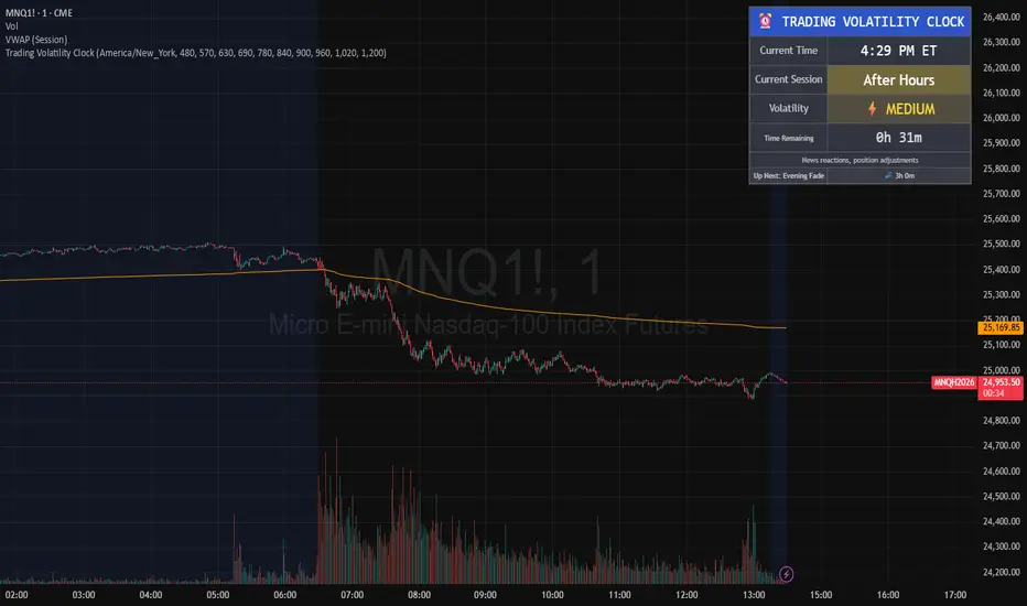
Trading Volatility Clock⏰ TRADING VOLATILITY CLOCK - Know When the Action Happens (Anywhere in the World)
A real-time session tracker with multi-timezone support for active traders who need to know when US market volatility strikes - no matter where they are in the world. Perfect for day traders, scalpers, and anyone trading liquid US markets.
══════════════════════════════════════════════════════
📊 WHAT IT DOES
This indicator displays a live clock showing:
- Current time in YOUR selected timezone (10 major timezones supported)
- Active US market session with color-coded volatility levels
- Countdown timer showing time remaining in current session
- Preview of the next upcoming session
- Optional alerts when entering high-volatility periods
══════════════════════════════════════════════════════
🌍 MULTI-TIMEZONE SUPPORT
SESSIONS ALWAYS TRACK US MARKET HOURS (Eastern Time):
No matter which timezone you select, the sessions always trigger at the correct US market times. Perfect for international traders who want to:
• See their local time while tracking US market sessions
• Know exactly when US volatility hits in their timezone
• Plan their trading day around US market hours
SUPPORTED TIMEZONES:
• America/New_York (ET) - Eastern Time
• America/Chicago (CT) - Central Time
• America/Los_Angeles (PT) - Pacific Time
• Europe/London (GMT) - Greenwich Mean Time
• Europe/Berlin (CET) - Central European Time
• Asia/Tokyo (JST) - Japan Standard Time
• Asia/Shanghai (CST) - China Standard Time
• Asia/Hong_Kong (HKT) - Hong Kong Time
• Australia/Sydney (AEDT) - Australian Eastern Time
• UTC - Coordinated Universal Time
EXAMPLE: A trader in Tokyo selects "Asia/Tokyo"
• Clock shows: 11:30 PM JST
• Session shows: "Opening Drive" 🔥 HIGH
• They know: US market just opened (9:30 AM ET in New York)
══════════════════════════════════════════════════════
🎯 WHY IT'S USEFUL
Whether you trade futures, high-volume stocks, or ETFs, volatility isn't constant throughout the day. Knowing WHEN to expect movement is critical:
🔥 HIGH VOLATILITY (Red):
• Opening Drive (9:30-10:30 AM ET) - Highest volume of the day
• Power Hour (3:00-4:00 PM ET) - Second-highest volume, final push
⚡ MEDIUM VOLATILITY (Yellow):
• Pre-Market (8:00-9:30 AM ET) - Building momentum
• Lunch Return (1:00-2:00 PM ET) - Traders returning
• Afternoon Session (2:00-3:00 PM ET) - Trend continuation
• After Hours (4:00-5:00 PM ET) - News reactions
💤 LOW VOLATILITY (Gray):
• Overnight Grind (12:00-8:00 AM ET) - Thin volume
• Mid-Morning Chop (10:30-11:30 AM ET) - Ranges form
• Lunch Hour (11:30 AM-1:00 PM ET) - Dead zone
• Evening Fade (5:00-8:00 PM ET) - Volume dropping
══════════════════════════════════════════════════════
⚙️ CUSTOMIZATION OPTIONS
TIMEZONE SETTINGS:
• Select from 10 major timezones worldwide
• Clock automatically displays in your local time
• Sessions remain locked to US market hours
SESSION TIME CUSTOMIZATION:
• Every session boundary is adjustable (in minutes from midnight ET)
• Perfect for traders who define sessions differently
• Advanced users can create custom volatility schedules
DISPLAY OPTIONS:
• Toggle next session preview on/off
• Enable/disable high volatility alerts
• Clean, unobtrusive table display in top-right corner
══════════════════════════════════════════════════════
💡 HOW TO USE
1. Add indicator to any chart (works on all timeframes)
2. Select your timezone in Settings → Timezone Settings
3. Set your chart to 1-minute timeframe for real-time updates
4. Customize session times if needed (Settings → Session Time Customization)
5. Watch the top-right corner for live session tracking
TRADING APPLICATIONS:
• Avoid trading during dead zones (lunch hour, mid-morning chop)
• Increase position size during high volatility windows
• Set alerts for Opening Drive and Power Hour
• Plan your trading day around US market volatility schedule
• International traders can track US sessions in their local time
══════════════════════════════════════════════════════
🎓 EDUCATIONAL VALUE
This indicator teaches traders:
• Market microstructure and volume patterns
• Why certain times produce better opportunities
• How institutional flows create intraday patterns
• The importance of timing in active trading
• How to adapt US market trading to any timezone
══════════════════════════════════════════════════════
⚠️ IMPORTANT NOTES
- Works best on 1-minute charts for frequent updates
- Sessions are ALWAYS based on US Eastern Time (ET)
- Timezone selection only changes the clock display
- Clock updates when new bar closes (not tick-by-tick)
- Alerts trigger once per bar when enabled
- Perfect for international traders tracking US markets
══════════════════════════════════════════════════════
📈 BEST USED WITH
- High-volume US stocks: TSLA, NVDA, AAPL, AMD, META
- Major US ETFs: SPY, QQQ, IWM, DIA
- US Futures: ES, NQ, RTY, YM, MES, MNQ
- Any liquid US instrument with clear intraday volume patterns
══════════════════════════════════════════════════════
🌏 FOR INTERNATIONAL TRADERS
This tool is specifically designed for traders outside the US who need to:
• Track US market sessions in their local timezone
• Know when to be at their desk for US volatility
• Avoid waking up for low-volatility periods
• Maximize trading efficiency around US market hours
No more timezone confusion. No more missing the opening bell. Just set your timezone and trade with confidence.
══════════════════════════════════════════════════════
This is an open-source educational tool. Feel free to modify and adapt to your trading style!
Happy Trading! 🚀
Predicted Funding RatesOverview
The Predicted Funding Rates indicator calculates real-time funding rate estimates for perpetual futures contracts on Binance. It uses triangular weighting algorithms on multiple different timeframes to ensure an accurate prediction.
Funding rates are periodic payments between long and short position holders in perpetual futures markets
If positive, longs pay shorts (usually bullish)
If negative, shorts pay longs (usually bearish)
This is a prediction. Actual funding rates depend on the instantaneous premium index, derived from bid/ask impacts of futures. So whilst it may imitate it similarly, it won't be completely accurate.
This only applies currently to Binance funding rates, as HyperLiquid premium data isn't available. Other Exchanges may be added if their premium data is uploaded.
Methods
Method 1: Collects premium 1-minunute data using triangular weighing over 8 hours. This granular method fills in predicted funding for 4h and less recent data
Method 2: Multi-time frame approach. Daily uses 1 hour data in the calculation, 4h + timeframes use 15M data. This dynamic method fills in higher timeframes and parts where there's unavailable premium data on the 1min.
How it works
1) Premium data is collected across multiple timeframes (depending on the timeframe)
2) Triangular weighing is applied to emphasize recent data points linearly
Tri_Weighing = (data *1 + data *2 + data *3 + data *4) / (1+2+3+4)
3) Finally, the funding rate is calculated
FundingRate = Premium + clamp(interest rate - Premium, -0.05, 0.05)
where the interest rate is 0.01% as per Binance
Triangular weighting is calculated on collected premium data, where recent data receives progressively higher weight (1, 2, 3, 4...). This linear weighting scheme provides responsiveness to recent market conditions while maintaining stability, similar to an exponential moving average but with predictable, linear characteristics
A visual representation:
Data points: ──────────────>
Weights: 1 2 3 4 5
Importance: ▂ ▃ ▅ ▆ █
How to use it
For futures traders:
If funding is trending up, the market can be interpreted as being in a bull market
If trending down, the market can be interpreted as being in a bear market
Even used simply, it allows you to gauge roughly how well the market is performing per funding. It can basically be gauged as a sentiment indicator too
For funding rate traders:
If funding is up, it can indicate a long on implied APR values
If funding is down, it can indicate a short on implied APR values
It also includes an underlying APR, which is the annualized funding rate. For Binance, it is current funding * (24/8) * 365
For Position Traders: Monitor predicted funding rates before entering large positions. Extremely high positive rates (>0.05% for 8-hour periods) suggest overleveraged longs and potential reversal risk. Conversely, extreme negative rates indicate shorts dominance
Table:
Funding rate: Gives the predicted funding rate as a percentage
Current premium: Displays the current premium (difference between perpetual futures price and the underlying spot) as a percentage
Funding period: You can choose between 1 hour funding (HyperLiquid usually) and 8 hour funding (Binance)
APR: Underlying annualized funding rate
What makes it original
Whilst some predicted funding scripts exist, some aren't as accurate or have gaps in data. And seeing as funding values are generally missing from TV tickers, this gives traders accessibility to the script when they would have to use other platforms
Notes
Currently only compatible with symbols that have Binance USDT premium indices
Optimal accuracy is found on timeframes that are 4H or less. On higher timeframes, the accuracy drops off
Actual funding rates may differ
Inputs
Funding Period: Choose between "8 Hour" (standard Binance cycle) or "1 Hour" (divides the 8-hour rate by 8 for granular comparison)
Plot Type: Display as "Funding Rate" (percentage per interval) or "APR" (annualized rate calculated as 8-hour rate × 3 × 365)
Table: Toggle the information table showing current funding rate, premium, funding period, and APR in the top-right corner
Positive Colour: Sets the colour for positive funding rates where longs pay shorts (default: #00ffbb turquoise)
Negative Colour: Sets the colour for negative funding rates where shorts pay longs (default: red)
Table Background: Controls the background colour and transparency of the information table (default: transparent dark blue)
Table Text Colour: Sets the colour for all text labels in the information table (default: white)
Table Text Size: Controls font size with options from Tiny to Huge, with Small as the default balance of readability and space

TimeMapTimeMap is a visual price-reference indicator designed to help traders rapidly visualize how current price levels relate to significant historical closing prices. It overlays your chart with reference lines representing past weekly, monthly, quarterly (3-month), semi-annual (6-month), and annual closing prices. By clearly plotting these historical price references, TimeMap helps traders quickly gauge price position relative to historical market structure, aiding in the identification of trends, support/resistance levels, and potential reversals.
How it Works:
The indicator calculates the precise number of historical bars corresponding to weekly, monthly, quarterly, semi-annual, and annual intervals, dynamically adjusting according to your chart’s timeframe (intraday, daily, weekly, monthly) and chosen market type (Stocks US, Crypto, Forex, or Futures). Historical closing prices from these periods are plotted directly on your chart as horizontal reference lines.
For intraday traders, the script accurately calculates historical offsets considering regular and extended trading sessions (e.g., pre-market and after-hours sessions for US stocks), ensuring correct positioning of historical lines.
User-Configurable Inputs Explained in Detail:
Market Type:
Allows you to specify your trading instrument type, automatically adjusting calculations for:
- Stocks US (default): 390 minutes per regular session (780 minutes if extended hours enabled), 5 trading days/week.
- Crypto: 1440 minutes/day, 7 trading days/week.
- Forex: 1440 minutes/day, 5 trading days/week.
- Futures: 1320 minutes/day, 5 trading days/week.
Show Weekly Close:
When enabled, plots a line at the exact closing price from one week ago. Provides short-term context and helps identify recent price momentum.
Show Monthly Close:
When enabled, plots a line at the exact closing price from one month ago. Helpful for evaluating medium-term price positioning and monthly trend strength.
Show 3-Month Close:
When enabled, plots a line at the exact closing price from three months ago. Useful for assessing quarterly market shifts, intermediate trend changes, and broader market sentiment.
Show 6-Month Close:
When enabled, plots a line at the exact closing price from six months ago. Useful for identifying semi-annual trends, significant price pivots, and longer-term support/resistance levels.
Show 1-Year Close:
When enabled, plots a line at the exact closing price from one year ago. Excellent for assessing long-term market direction and key annual price levels.
Enable Smoothing:
Activates a Simple Moving Average (SMA) smoothing of historical reference lines, reducing volatility and providing clearer visual references. Recommended for traders preferring less volatile reference levels.
Smoothing Length:
Determines the number of bars used in calculating the SMA smoothing of historical lines. Higher values result in smoother but slightly delayed reference lines; lower values offer more immediate yet more volatile levels.
Use Extended Hours (Intraday Only):
When enabled (only applicable for Stocks US), it accounts for pre-market and after-hours trading sessions, providing accurate intraday historical line calculations based on extended sessions (typically 780 minutes/day total).
Important Notes and Compliance:
- This indicator does not provide trading signals, recommendations, or predictions. It serves purely as a visual analytical tool to supplement traders’ existing methods.
- Historical lines plotted are strictly based on past available price data; the indicator never accesses future data or data outside the scope of Pine Script’s standard capabilities.
- The script incorporates built-in logic to avoid runtime errors if insufficient historical data exists for a selected timeframe, ensuring robustness even with limited historical bars.
- TimeMap is original work developed exclusively by Julien Eche (@Julien_Eche). It does not reuse or replicate third-party or existing open-source scripts.
Recommended Best Practices:
- Use TimeMap as a complementary analytical reference, not as a standalone strategy or trade decision-making tool.
- Adapt displayed historical periods and smoothing settings based on your trading style and market approach.
- Default plot colors are optimized for readability on dark-background charts; adjust as necessary according to your preference and chart color scheme.
This script is published open-source to benefit the entire TradingView community and fully complies with all TradingView script publishing rules and guidelines.
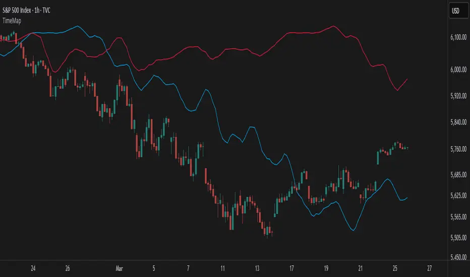
Easy CotHow to Use the Commitment of Traders (COT) Report for Market Analysis
The Commitment of Traders (COT) report is a weekly publication by the Commodity Futures Trading Commission (CFTC) that breaks down the open interest in various futures markets. It categorizes traders into three main groups: Commercials, Non-Commercials, and Retail Traders (Non-Reportable positions). Understanding and analyzing the COT report can provide insights into market sentiment and potential reversals, especially in commodity, currency, and stock index futures.
Key Components of the COT Report
Commercials (Hedgers)
These are entities involved in the production or consumption of the underlying asset. For example, oil producers might hedge by selling oil futures to lock in prices, while airlines might buy futures to hedge against rising prices.
Commercials typically act as hedgers, so their positions can indicate the need for protection rather than speculative intent. Because they are less price-sensitive, their positions are usually opposite to the trend near market reversals.
Non-Commercials (Large Speculators)
This group includes hedge funds, asset managers, and large traders who take speculative positions to profit from price movements.
Non-Commercials are often trend-followers, meaning they increase long positions in an uptrend and short positions in a downtrend. When Non-Commercials become extremely bullish or bearish, it may signal a potential market reversal.
Retail Traders (Non-Reportable Positions)
These are smaller individual traders whose positions are too small to be reported individually.
Retail traders tend to be less experienced and are often on the wrong side of major market moves, so extreme positions by retail traders can sometimes signal a market turning point.
How to Interpret the COT Data
1. Identify Extreme Positions
Extreme Long or Short Positions: When a group reaches a historically extreme level of long or short positions, it often signals a potential reversal. For instance, if Non-Commercials are overwhelmingly long, it may indicate that the uptrend is overextended, and a reversal could be near.
Contrarian Indicator: Since Retail Traders are often on the wrong side, you may look for signals where they are extremely long or short, indicating a possible reversal in the opposite direction.
2. Look for Divergences
Divergence Between Groups: If Non-Commercials (speculators) and Retail Traders are moving in opposite directions, it could indicate that a trend is losing momentum and a reversal is possible.
Commercials vs. Non-Commercials: Commercials are often positioned opposite to Non-Commercials. If there’s a divergence where Non-Commercials are highly bullish, but Commercials are increasingly bearish, it might suggest a coming reversal.
3. Trend Confirmation and Reversal Signals
Trend Confirmation: If both Non-Commercials and Retail Traders are aligned in one direction, it might confirm the trend. However, keep in mind that such alignment may signal the later stages of a trend.
Reversal Signals: Look for signs when Non-Commercials are reaching a peak in one direction while Retail Traders peak in the opposite. Such situations can often indicate that the current trend is close to exhaustion.
Using the COT Report in Trading Strategies
Contrarian Trading Strategy
Extreme Positions as Reversal Signals: Use COT data to identify extreme positions. For instance, if Non-Commercials have a very high long position in a commodity, it might suggest that a bullish trend is overextended and a bearish reversal could be near.
Retail Trader Extremes: If Retail Traders are heavily long or short, consider taking the opposite position once you have additional confirmation signals (e.g., technical indicators).
Following the Trend with Large Speculators
Non-Commercials tend to be trend-followers, so if you see them increasingly long (or short) on an asset, it could be a signal to follow the trend until extreme levels are reached.
Using Divergences for Entry and Exit Points
Entry: If Non-Commercials are long, but Retail Traders are heavily short, consider entering a long position as it may confirm the trend.
Exit: If Non-Commercials begin to reduce their positions while Retail Traders increase theirs, it might be time to consider exiting, as the trend could be losing momentum.

Globex, Extended, Daily, Weekly, Monthly, Yearly Range* Adds Right Side Only Price Line & Labels for Tracking without Extending Both Sides
* Tracks Current, Previous, and Two Previous Globex Sessions/ Futures:
* Tracks Current, Previous, and Two Previous Extended Session/ Stocks:
* Tracks Current, Previous, Two, & Three Previous Day Session/ Equities:
* Tracks Current, Last, Two, Three, Four, & Five Week Session/ Equities:
* Tracks Current, Last, Two, Three, Four, & Five Month Session/ Equities:
* Tracks Current, Last, Two, Three, Four, & Five Year Session/ Equities:
* Allows Custom Range on Globex, Extended, & Daily Sessions
* Allows Custom Range on Weekly, Monthly, & Yearly Sessions
* Lines & Labels Are Not Visible on Chart Scales
* Reversible Text & Background Color
* Lines Extend Accordingly with Range
* Labels show Price & Percent Change
* Background Colors should match Chart Color to avoid Overlapping Text & Labels
* Lines have Offset Extension
* Labels have Offset Extension
* Globex Session is only visible on Futures & if Current Timeframe is Intraday
* Extended Session is only visible on Stocks & if Current Timeframe is Intraday
* Daily, Weekly, Monthly, & Yearly Sessions are visible on All Symbols & All Timeframes
* Globex, Extended, & Regular use their Default Time Sessions but allow Customization
* For Back Testing Default Sessions, switch over on the Menu to Style and Turn On/Off their Background Color; Any Area on the Chart Without Background Color is Regular Session
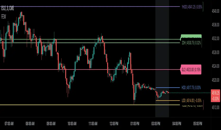
LibraryCOTLibrary "LibraryCOT"
This library provides tools to help Pine programmers fetch Commitment of Traders (COT) data for futures.
rootToCFTCCode(root)
Accepts a futures root and returns the relevant CFTC code.
Parameters:
root : Root prefix of the future's symbol, e.g. "ZC" for "ZC1!"" or "ZCU2021".
Returns: The part of a COT ticker corresponding to `root`, or "" if no CFTC code exists for the `root`.
currencyToCFTCCode(curr)
Converts a currency string to its corresponding CFTC code.
Parameters:
curr : Currency code, e.g., "USD" for US Dollar.
Returns: The corresponding to the currency, if one exists.
optionsToTicker(includeOptions)
Returns the part of a COT ticker using the `includeOptions` value supplied, which determines whether options data is to be included.
Parameters:
includeOptions : A "bool" value: 'true' if the symbol should include options and 'false' otherwise.
Returns: The part of a COT ticker: "FO" for data that includes options and "F" for data that doesn't.
metricNameAndDirectionToTicker(metricName, metricDirection)
Returns a string corresponding to a metric name and direction, which is one component required to build a valid COT ticker ID.
Parameters:
metricName : One of the metric names listed in this library's chart. Invalid values will cause a runtime error.
metricDirection : Metric direction. Possible values are: "Long", "Short", "Spreading", and "No direction". Valid values vary with metrics. Invalid values will cause a runtime error.
Returns: The part of a COT ticker ID string, e.g., "OI_OLD" for "Open Interest" and "No direction", or "TC_L" for "Traders Commercial" and "Long".
typeToTicker(metricType)
Converts a metric type into one component required to build a valid COT ticker ID. See the "Old and Other Futures" section of the CFTC's Explanatory Notes for details on types.
Parameters:
metricType : Metric type. Accepted values are: "All", "Old", "Other".
Returns: The part of a COT ticker.
convertRootToCOTCode(mode, convertToCOT)
Depending on the `mode`, returns a CFTC code using the chart's symbol or its currency information when `convertToCOT = true`. Otherwise, returns the symbol's root or currency information. If no COT data exists, a runtime error is generated.
Parameters:
mode : A string determining how the function will work. Valid values are:
"Root": the function extracts the futures symbol root (e.g. "ES" in "ESH2020") and looks for its CFTC code.
"Base currency": the function extracts the first currency in a pair (e.g. "EUR" in "EURUSD") and looks for its CFTC code.
"Currency": the function extracts the quote currency ("JPY" for "TSE:9984" or "USDJPY") and looks for its CFTC code.
"Auto": the function tries the first three modes (Root -> Base Currency -> Currency) until a match is found.
convertToCOT : "bool" value that, when `true`, causes the function to return a CFTC code. Otherwise, the root or currency information is returned. Optional. The default is `true`.
Returns: If `convertToCOT` is `true`, the part of a COT ticker ID string. If `convertToCOT` is `false`, the root or currency extracted from the current symbol.
COTTickerid(COTType, CTFCCode, includeOptions, metricName, metricDirection, metricType)
Returns a valid TradingView ticker for the COT symbol with specified parameters.
Parameters:
COTType : A string with the type of the report requested with the ticker, one of the following: "Legacy", "Disaggregated", "Financial".
CTFCCode : The for the asset, e.g., wheat futures (root "ZW") have the code "001602".
includeOptions : A boolean value. 'true' if the symbol should include options and 'false' otherwise.
metricName : One of the metric names listed in this library's chart.
metricDirection : Direction of the metric, one of the following: "Long", "Short", "Spreading", "No direction".
metricType : Type of the metric. Possible values: "All", "Old", and "Other".
Returns: A ticker ID string usable with `request.security()` to fetch the specified Commitment of Traders data.

Dominant Cycle Tuned RsiIntroduction
Adaptive technical indicators are importants in a non stationary market, the ability to adapt to a situation can boost the efficiency of your strategy. A lot of methods have been proposed to make technical indicators "smarters" , from the use of variable smoothing constant for exponential smoothing to artificial intelligence.
The dominant cycle tuned rsi depend on the dominant cycle period of the market, such method allow the rsi to return accurate peaks and valleys levels. This indicator is an estimation of the cycle finder tuned rsi proposed by Lars von Thienen published in Decoding the Hidden Market Rhythm/Fine-tuning technical indicators using the dominant market vibration/2010 using the cycle measurement method described by John F.Ehlers in Cybernetic Analysis for Stocks and Futures .
The following section is for information purpose only, it can be technical so you can skip directly to the The Indicator section.
Frequency Estimation and Maximum Entropy Spectral Analysis
“Looks like rain,” said Tom precipitously.
Tom would have been a great weather forecaster, but market patterns are more complex than weather ones. The ability to measure dominant cycles in a complex signal is hard, also a method able to estimate it really fast add even more challenge to the task. First lets talk about the term dominant cycle , signals can be decomposed in a sum of various sine waves of different frequencies and amplitudes, the dominant cycle is considered to be the frequency of the sine wave with the highest amplitude. In general the highest frequencies are those who form the trend (often called fundamentals) , so detrending is used to eliminate those frequencies in order to keep only mid/mid - highs ones.
A lot of methods have been introduced but not that many target market price, Lars von Thienen proposed a method relying on the following processing chain :
Lars von Thienen Method = Input -> Filtering and Detrending -> Discrete Fourier Transform of the result -> Selection using Bartels statistical test -> Output
Thienen said that his method is better than the one proposed by Elhers. The method from Elhers called MESA was originally developed to interpret seismographic information. This method in short involve the estimation of the phase using low amount of information which divided by 360 return the frequency. At first sight there are no relations with the Maximum entropy spectral estimation proposed by Burg J.P. (1967). Maximum Entropy Spectral Analysis. Proceedings of 37th Meeting, Society of Exploration Geophysics, Oklahoma City.
You may also notice that these methods are plotted in the time domain where more classic method such as : power spectrum, spectrogram or FFT are not. The method from Elhers is the one used to tune our rsi.
The Indicator
Our indicator use the dominant cycle frequency to calculate the period of the rsi thus producing an adaptive rsi . When our adaptive rsi cross under 70, price might start a downtrend, else when our adaptive rsi crossover 30, price might start an uptrend. The alpha parameter is a parameter set to be always lower than 1 and greater than 0. Lower values of alpha minimize the number of detected peaks/valleys while higher ones increase the number of those. 0.07 for alpha seems like a great parameter but it can sometimes need to be changed.
The adaptive indicator can also detect small top/bottoms of small periods
Of course the indicator is subject to failures
At the end it is totally dependent of the dominant cycle estimation, which is still a rough method subject to uncertainty.
Conclusion
Tuning your indicator is a great way to make it adapt to the market, but its also a complex way to do so and i'm not that convinced about the complexity/result ratio. The version using chart background will be published separately.
Feel free to tune your indicators with the estimator from elhers and see if it provide a great enhancement :)
Thanks for reading !
References
for the calculation of the dominant cycle estimator originally from www.davenewberg.com
Decoding the Hidden Market Rhythm (2010) Lars von Thienen
Ehlers , J. F. 2004 . Cybernetic Analysis for Stocks and Futures: Cutting-Edge DSP Technology to Improve Your Trading . Wiley

Universal Sentiment Oscillator with Trade RecommendationsUniversal Sentiment Oscillator & Strategy Guide
Summary
This all-in-one indicator is designed to be a comprehensive co-pilot for your trading journey. It moves beyond simple buy/sell signals by analyzing the underlying market sentiment and providing a dynamic, risk-assessed guide of potential trading strategies. Whether you're a novice learning the ropes or an expert seeking confirmation, this tool provides a structured framework for making smarter, more informed decisions in stocks, options, and futures.
How It Works
The core of the indicator is the Sentiment Oscillator, which calculates a score from -5 (Extremely Bearish) to +5 (Extremely Bullish) on every bar. This isn't just a single measurement; it's a weighted aggregate of several key technical conditions:
Trend Analysis: Price position relative to the 20, 50, and 200 EMAs.
Momentum Analysis: The current RSI value.
Hybrid Analysis: The state of the MACD and its signal line.
These factors are intelligently combined and normalized to produce a single, intuitive sentiment score, giving you an at-a-glance understanding of the market's pulse.
Core Features
Dynamic Trade Recommendation Table:
The informational heart of the indicator. This on-chart table provides a list of potential trades perfectly aligned with the current sentiment score.
Risk-Ranked Strategies:
All suggested trades are logically ordered by risk, helping you quickly identify strategies that match your comfort level.
Adjusted Trade Suggestions:
The indicator analyzes sentiment momentum (the score vs. its signal line) to provide proactive, forward-looking trade ideas based on where the market might be heading next.
Customizable Trading Styles:
Tell the indicator if you are a Conservative, Neutral, or Aggressive trader, and the "Adjusted Trade Suggestion" will automatically tailor its recommendations to your personal risk preference.
Context-Aware Futures Mode:
When viewing a futures contract, enable this mode to switch all recommendations from stock/options to futures-specific actions (e.g., "Cautious Long," "Monitor Range").
Predictive Sentiment Cone:
Visualize the potential short-term path of sentiment based on current momentum, helping you anticipate future conditions.
Fully Customizable:
Every parameter—from EMA lengths to trade filters—can be adjusted, allowing you to fine-tune the indicator to your exact specifications.
How to Use This Indicator
This tool is flexible and can be integrated into many trading systems. Here is a powerful, professional approach:
Top-Down Analysis (for Swing or Position Trading):
Establish the Trend: Start on the higher timeframes (Monthly, Weekly, Daily). Use the oscillator's color and score to define the dominant, long-term market sentiment. You only want to look for trades that align with this macro trend.
Refine the Entry: Drop down to the medium timeframes (4-Hour, 1-Hour). Wait for the sentiment on these charts to come into alignment with the higher-timeframe trend. This pullback or consolidation is your "zone of interest."
Pinpoint the Execution: Move to a lower timeframe (e.g., 15-Minute). Use the Adjusted Trade Suggestion and Sentiment Momentum to find a precise entry as momentum begins to shift back in the direction of the primary trend. You can set alerts on the oscillator's zero-line for early warnings of a sentiment shift.
As a Confirmation Tool: If you have an existing trade idea, use the indicator to validate it. Does the sentiment score align with your bullish or bearish thesis? Does the momentum confirm that now is a good time to enter?
As an Idea Generation Tool: Unsure what to trade? Browse different assets and let the indicator's "Primary Trades" and "Adjusted Trade Suggestion" present you with a list of risk-assessed ideas that you can then investigate further.
Disclaimer: This is an analysis tool and should not be considered financial advice. All forms of trading involve substantial risk. You should not trade with money you cannot afford to lose. Always perform your own due diligence and use this indicator as one component of a complete trading plan.

Risk TrackerThis Risk Tracker Pine Script provides traders with a customizable tool for tracking and managing trade risk directly on their chart. The script is designed to accommodate both futures and crypto trades, allowing you to monitor risk and reward parameters, adjust contract sizes, and manage leverage in real-time.
Key Features:
1. Trade Direction and Risk-Reward Ratio:
• Select between Long or Short trade directions.
• Set a custom Risk-Reward Ratio (RRR) to calculate potential profit and loss levels based on your trade setup.
2. Customizable Parameters:
• Input fields for contract size, leverage, margin, and maximum drawdown allow you to adjust the risk settings depending on the market you are trading.
• You can toggle between using a dollar-based or percentage-based risk calculation depending on whether you’re trading futures (USD-based) or crypto.
3. Real-time Stop-Loss and Take-Profit Calculation:
• The script automatically calculates and draws the Stop-Loss (SL) and Take-Profit (TP) levels on the chart based on your entry price and selected risk settings.
• The color of the SL and TP lines is customizable, allowing you to visually distinguish profit and loss levels.
4. Historical Price Levels:
• If there is no active trade, the script scans historical price data to find the last instances when the price hit the predefined stop-loss or take-profit levels, helping you understand past price behavior.
5. Risk Management Table:
• A summary table is displayed on the chart, showing the key metrics of your trade, including:
• Tick value and Dollar value for futures.
• Margin and Leverage for crypto.
• Risk-Reward Ratio, Entry price, Risk and Profit in USD or percentage terms.
• The table dynamically updates based on the current trade status.
6. Extended Chart Visualization:
• Option to extend the SL and TP lines to the left of the chart, allowing you to easily view these levels across multiple timeframes and bars.
This script helps ensure you are always aware of your trade’s risk profile, providing a clear and visual representation of potential profit and loss, both in terms of percentage and dollar value. Ideal for futures and crypto traders who rely on precise risk management to maintain profitability.

LibraryCOT_NZLibrary "LibraryCOT_NZ"
This library provides tools to help Pine programmers fetch Commitment of Traders (COT) data for futures.
rootToCFTCCode(root)
Accepts a futures root and returns the relevant CFTC code.
Parameters:
root (simple string) : Root prefix of the future's symbol, e.g. "ZC" for "ZC1!"" or "ZCU2021".
Returns: The part of a COT ticker corresponding to `root`, or "" if no CFTC code exists for the `root`.
currencyToCFTCCode(currency)
Converts a currency string to its corresponding CFTC code.
Parameters:
currency (simple string)
Returns: The corresponding to the currency, if one exists.
optionsToTicker(includeOptions)
Returns the part of a COT ticker using the `includeOptions` value supplied, which determines whether options data is to be included.
Parameters:
includeOptions (simple bool) : A "bool" value: 'true' if the symbol should include options and 'false' otherwise.
Returns: The part of a COT ticker: "FO" for data that includes options and "F" for data that doesn't.
metricNameAndDirectionToTicker(metricName, metricDirection)
Returns a string corresponding to a metric name and direction, which is one component required to build a valid COT ticker ID.
Parameters:
metricName (simple string) : One of the metric names listed in this library's chart. Invalid values will cause a runtime error.
metricDirection (simple string) : Metric direction. Possible values are: "Long", "Short", "Spreading", and "No direction". Valid values vary with metrics. Invalid values will cause a runtime error.
Returns: The part of a COT ticker ID string, e.g., "OI_OLD" for "Open Interest" and "No direction", or "TC_L" for "Traders Commercial" and "Long".
typeToTicker(metricType)
Converts a metric type into one component required to build a valid COT ticker ID. See the "Old and Other Futures" section of the CFTC's Explanatory Notes for details on types.
Parameters:
metricType (simple string) : Metric type. Accepted values are: "All", "Old", "Other".
Returns: The part of a COT ticker.
convertRootToCOTCode(mode, convertToCOT)
Depending on the `mode`, returns a CFTC code using the chart's symbol or its currency information when `convertToCOT = true`. Otherwise, returns the symbol's root or currency information. If no COT data exists, a runtime error is generated.
Parameters:
mode (simple string) : A string determining how the function will work. Valid values are:
"Root": the function extracts the futures symbol root (e.g. "ES" in "ESH2020") and looks for its CFTC code.
"Base currency": the function extracts the first currency in a pair (e.g. "EUR" in "EURUSD") and looks for its CFTC code.
"Currency": the function extracts the quote currency ("JPY" for "TSE:9984" or "USDJPY") and looks for its CFTC code.
"Auto": the function tries the first three modes (Root -> Base Currency -> Currency) until a match is found.
convertToCOT (simple bool) : "bool" value that, when `true`, causes the function to return a CFTC code. Otherwise, the root or currency information is returned. Optional. The default is `true`.
Returns: If `convertToCOT` is `true`, the part of a COT ticker ID string. If `convertToCOT` is `false`, the root or currency extracted from the current symbol.
COTTickerid(COTType, CFTCCode, includeOptions, metricName, metricDirection, metricType)
Returns a valid TradingView ticker for the COT symbol with specified parameters.
Parameters:
COTType (simple string) : A string with the type of the report requested with the ticker, one of the following: "Legacy", "Disaggregated", "Financial".
CFTCCode (simple string)
includeOptions (simple bool) : A boolean value. 'true' if the symbol should include options and 'false' otherwise.
metricName (simple string) : One of the metric names listed in this library's chart.
metricDirection (simple string) : Direction of the metric, one of the following: "Long", "Short", "Spreading", "No direction".
metricType (simple string) : Type of the metric. Possible values: "All", "Old", and "Other".
Returns: A ticker ID string usable with `request.security()` to fetch the specified Commitment of Traders data.
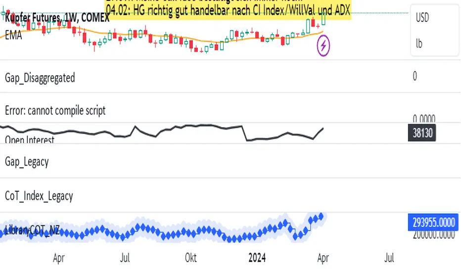
Weis V5 zigzag jayySomehow, I deleted version 5 of the zigzag script. Same name. I have added some older notes describing how the Weis Wave works.
I have also changed the date restriction that stopped the script from working after Dec 31, 2022.
What you see here is the Weis zigzag wave plotted directly on the price chart. This script is the companion to the Weis cumulative wave volume script.
What is a Weis wave? David Weis has been recognized as a Wyckoff method analyst he has written two books one of which, Trades About to Happen, describes the evolution of the now-popular Weis wave. The method employed by Weis is to identify waves of price action and to compare the strength of the waves on characteristics of wave strength. Chief among the characteristics of strength is the cumulative volume of the wave. There are other markers that Weis uses as well for example how the actual price difference between the start of the Weis wave from start to finish. Weis also uses time, particularly when using a Renko chart
David Weis did a futures io video which is a popular source of information about his method. (Search David Weis and futures.io. I strongly suggest you also read “Trades About to Happen” by David Weis.
This will get you up and running more quickly when studying charts. However, you should choose the Traditional method to be true to David Weis technique as described in his book "Trades About to Happen" and in the Futures IO Webcast featuring David Weis
. The Weis pip zigzag wave shows how far in terms of bar close price a Weis wave has traveled through the duration of a Weis wave. The Weis zigzag wave is used in combination with the Weis cumulative volume wave. The two waves should be set to the same "wave size".
To use this script, you must set the wave size: Using the traditional Weis method simply enter the desired wave size in the box "How should wave size be calculated", in this example I am using a traditional wave size of .25. Each wave for each security and each timeframe requires its own wave size. Although not the traditional method devised by David Weis a more automatic way to set wave size would be to use Average True Range (ATR). Using ATR is not the true Weis method but it does give you similar waves and, importantly, without the hassle described above. Once the Weis wave size is set then the zigzag wave will be shown with volume. Because Weis used the closing price of a wave to define waves a line Bar highs and bar lows are not captured by the Weis Wave. The default script setting is now cumulative volume waves using an ATR of 7 and a multiplication factor of .5.
To display volume in a way that does not crowd out neighbouring volumes Weis displayed volume as a maximum of 3 digits (usually). Consider two Weis Wave volumes 176,895,570 and 2,654,763,889. To display wave volume as three digits it is necessary to take a number such as 176,895,570 and truncate it. 176,895,570 can be represented as 177 X 10 to the power of 6. The number displayed must also be relative to other numbers in the field. If the highest volume on the page is: 2,654,763,889 and with only three numbers available to display the result the value shown must be 265 (265 X 10 to the power of 7). Since 176,895,570 is an order of magnitude smaller than 2,654,763,889 therefore 175,895,570 must be shown as 18 instead of 177. In this way, the relative magnitudes of the two volumes can be understood. All numbers in the field of view must be truncated by the same order of magnitude to make the relative volumes understandable. The script attempts to calculate the order of magnitude value automatically. If you see a red number in the field of view it means the script has failed to do the calculation automatically and you should use the manual method – use the dialogue box “Calculate truncated wave value automatically or manually”. Scroll down from the automatic method and select manual. Once "manual" is selected the values displayed become the power values or multipliers for each wave.
Using the manual method you will select a “Multiplier” in the next dialogue box. Scan the field and select the largest value in the field of view (visible chart) is the multiplier of interest. If you select a lower number than the maximum value will see at least one red “up”. If you are too high you will see at least one red “down”. Scroll in the direction recommended or the values on the screen will be totally incorrect. With volume truncated to the highest order values, the eye can quickly get a feel for relative volumes. It also reduces the crowding and overlapping of values on the screen. You can opt to show the full volume to help get a sense of the magnitude of the true volumes.
How does the script determine if a Weis wave is continuing to grow or not?
The script evaluates the closing price of each new bar relative to the "Weis wave size". Suppose the current bar closes at a new low close, within the current down wave, at $30.00. If the Weis wave size is $0.10 then the algorithm will remember the $30.00 close and compare it to the close of the next bar. If the bar close price does not close equal to or lower than $30.00 or close equal to or higher than $30.10 then the wave is still a down wave with a current low of $30.00. This is true even if the bar low is less than $30.00 or the bar high is greater than 30.10 – only the bar’s closing price matters. If a bar's closing price climbs back up to a close of $30.11 then because the closing price has moved more than $0.10 (the Weis wave size) then that is a wave reversal with a new up-trending wave. In the above example if there was currently a downward trending wave and the bar closes were as follows $30.00, $30.09, $30.01, $30.05, $30.10 The wave direction would continue to stay downward trending until the close of $30.10 was achieved. As such $30.00 would be the low and the following closes $30.09, $30.01, $30.05 would be allocated to the new upward-trending wave. If however There was a series of bar closes like this $30.00, $30.09, $30.01, $30.05, $29.99 since none of the closes was equal to above the 10-cent reversal target of $30.10 but instead, a new Weis wave low was achieved ($29.99). As such the closes of $30.09, $30.01, $30.05 would all be attributed to the continued down-trending wave with a current low of $29.99, even though the closing price for the interim bars was above $30.00. Now that the Weis Wave low is now 429.99 then, in order to reverse this continued downtrend price will need to close at or above $30.09 on subsequent bar closes assuming now new low bar close is achieved. With large wave sizes, wave direction can be in limbo for many bars before a close either renews wave direction or reverses it and confirms wave direction as either a reversal or a continuation. On the zig-zag, a wave line and its volume will not be "printed" until a wave reversal is confirmed.
The wave attribution is similar when using other methods to define wave size. If ATR is used for wave size instead of a traditional wave constant size such as $0.10 or $2 or 2000 pips or ... then the wave size is calculated based on current ATR instead of the Weis wave constant (Traditional selected value).
I have the option to display pseudo-Ord volume. In truth, Ord used more traditional zig-zag pivots of bar highs and lows. Waves using closes as pivots can have some significant differences. This difference can be lessened by using smaller time frames and larger wave sizes.
There are other options such to display the delta price or pip size of a Weis Wave, the number of bars in a wave, and a few other options.

Volume Divergence Detector - COT EnhancedVolume Divergence Detector – COT Enhanced
This advanced indicator analyzes institutional vs retail money flow to uncover hidden market intent, focusing on Gold and Gold Futures.
Instead of relying on simple volume spikes, the script separates smart money (institutions, commercial hedgers, large speculators) from retail traders using a blend of:
Volume-based accumulation/distribution
Price momentum
RSI behavior
MACD divergence
Institutional-sized volume detection
Optional real CFTC Commitment of Traders (COT) data
The result is a dynamic money-flow model designed to expose who is truly controlling the market.
🔹 Institutional Flow Engine
Large-volume activity is tracked and converted into a smoothed institutional money line. Heavy volume is weighted more aggressively to highlight professional accumulation and distribution. When volume fades, flow naturally decays to avoid stale signals.
If enabled, weekly CFTC COT data is blended into the calculation (70% internal model, 30% real positioning), providing genuine futures-market confirmation for Gold.
Positive values indicate institutional buying.
Negative values indicate institutional selling.
🔹 Retail Flow Engine
Retail behavior is modeled using:
RSI momentum (retail follows trends)
MACD breakout behavior
Smaller volume spikes
Retail flow reacts faster and decays quicker, reflecting emotional trading and late entries. Extreme retail positioning often signals potential reversals.
🔹 Core Signals
The indicator automatically detects:
Institutional Takeover
When institutional flow crosses above retail.
Retail Takeover
When retail flow crosses above institutions (often a warning sign).
Bullish Setup
Institutions buying + retail selling.
Bearish Setup
Institutions selling + retail buying.
Extreme Divergence
Institutional and retail flows at opposite extremes. These zones often precede major reversals or powerful trend continuations.
Clear BUY / SELL labels appear directly on the chart, positioned dynamically using ATR to avoid candle overlap.
🔹 Visual Feedback
Background shading shows which side currently dominates
Extreme divergence adds special highlighting
Real-time labels display institutional and retail values
A built-in information table summarizes:
Institutional flow
Retail flow
Dominant side
Flow spread
Current signal
COT status
Everything updates live on the last bar.
🔹 Alerts Included
Custom alerts are provided for:
Institutional control
Retail control
Bullish setups
Bearish setups
Extreme divergence
Perfect for automation or hands-off monitoring.
⚠️ Important Notes
COT data works only on Gold Futures symbols.
Spot Gold uses volume-based estimation only.
Designed for directional bias and timing, not blind entries. Always confirm with structure and price action.
Created by xqweasdzxcv
A professional-grade money flow system built to follow smart capital instead of emotional traders.

Gamma of Gamma - AnticipationGamma of Gamma — Anticipation Engine
What if you could detect market inflections before they become obvious? Not react to momentum — anticipate the momentum itself.
"Gamma here refers to mathematical acceleration (2nd derivative), NOT options Gamma"
Gamma of Gamma (GoG) operates one abstraction layer above conventional indicators. While RSI tells you what momentum did , GoG tells you what momentum is about to do . This is the difference between chasing price and positioning ahead of it.
Core Innovation: Traditional indicators measure first-order effects (price change) or second-order effects (momentum/acceleration). This system measures the third derivative — the rate of change of acceleration itself. When Gamma-of-Gamma reaches extremes, it signals that pressure dynamics are about to flip — often 2-5 bars before price visibly reacts.
Target Users: Discretionary traders, scalpers, and swing traders who want early positioning signals with statistical rigor. Effective on stocks, crypto, forex, and futures with meaningful volume data.
━━━━━━━━━━━━━━━━━━━━━━━━━━━━━━━━━━━━━━━━━━━
WHY THIRD-DERIVATIVE ANALYSIS?
━━━━━━━━━━━━━━━━━━━━━━━━━━━━━━━━━━━━━━━━━━━
The Hierarchy of Market Information
Most traders operate at the wrong level of abstraction:
• Price → What happened (lagging)
• Momentum → How fast it happened (still lagging)
• Gamma (2nd Derivative) → How momentum is changing (coincident)
• Gamma of Gamma (3rd Derivative) → How FAST that change is changing ( leading )
The third derivative captures inflection acceleration — the mathematical signature of regime transition. When GoG reaches extreme values, the market is telegraphing that current pressure dynamics are unsustainable.
Why This Beats RSI
RSI measures momentum magnitude. GoG measures momentum trajectory .
Consider this scenario: RSI reads 70 (overbought). Is the move exhausted or just getting started? RSI cannot tell you. GoG can — because it measures whether buying pressure is accelerating into the high RSI reading (continuation likely) or decelerating despite high RSI (reversal imminent).
RSI answers: "How strong was the move?"
GoG answers: "Is the move strengthening or weakening right now ?"
The first is historical. The second is predictive.
━━━━━━━━━━━━━━━━━━━━━━━━━━━━━━━━━━━━━━━━━━━
MATHEMATICAL FOUNDATION
━━━━━━━━━━━━━━━━━━━━━━━━━━━━━━━━━━━━━━━━━━━
Layer 1: Cumulative Volume Delta (CVD)
The foundation is order flow approximation:
• Up bar (close > prior close): Volume classified as buying pressure
• Down bar (close < prior close): Volume classified as selling pressure
• CVD = Running sum of signed volume
Interpretation: Rising CVD indicates net aggressive buying. Falling CVD indicates net aggressive selling. CVD divergence from price often precedes reversals.
Layer 2: Gamma (Second Derivative)
Gamma measures acceleration of order flow:
Formula: Gamma = CVD - 2×CVD + CVD
This is the discrete second derivative — the rate of change of the rate of change. When Gamma spikes positive, buying pressure is accelerating . When Gamma spikes negative, selling pressure is accelerating.
Layer 3: Gamma of Gamma (Third Derivative)
GoG measures jerk — the acceleration of acceleration:
Formula: GoG = Gamma - 2×Gamma + Gamma
Critical insight: Extreme GoG readings indicate that current pressure dynamics are reaching an inflection point. The system is "overextended" in its current trajectory and will likely revert or reverse.
Layer 4: Z-Score Normalization
Raw GoG values are normalized against their 50-period distribution:
Formula: GoG_Z = (GoG - Mean_50) / StdDev_50
Benefit: Z-scores are regime-adaptive. A "2.0" reading always means "2 standard deviations from normal" regardless of whether you're trading a penny stock or ES futures. This makes thresholds consistent across instruments and timeframes.
━━━━━━━━━━━━━━━━━━━━━━━━━━━━━━━━━━━━━━━━━━━
SIGNAL GENERATION LOGIC
━━━━━━━━━━━━━━━━━━━━━━━━━━━━━━━━━━━━━━━━━━━
Long Signal (Bullish Anticipation)
Triggers when:
• GoG Z-score < -Threshold (default -2.0)
• Volume > Average Volume × Minimum Multiple (default 1.2×)
Interpretation: Selling pressure acceleration has reached an extreme negative reading. The selling is "exhausting itself" — acceleration is peaking and will soon decelerate. Buyers are likely to step in.
Short Signal (Bearish Anticipation)
Triggers when:
• GoG Z-score > +Threshold (default +2.0)
• Volume > Average Volume × Minimum Multiple (default 1.2×)
Interpretation: Buying pressure acceleration has reached an extreme positive reading. The buying is "exhausting itself" — often occurs at blow-off tops, failed breakouts, or momentum climaxes.
Why Volume Confirmation?
Gamma acceleration in thin liquidity is meaningless noise. The volume filter ensures signals occur only when meaningful participation backs the pressure dynamics. This dramatically reduces false signals during low-activity periods.
━━━━━━━━━━━━━━━━━━━━━━━━━━━━━━━━━━━━━━━━━━━
CONFIDENCE ENGINE
━━━━━━━━━━━━━━━━━━━━━━━━━━━━━━━━━━━━━━━━━━━
Not all signals are equal. The Confidence Engine quantifies signal strength:
Confidence Calculation:
Confidence = 50 + ((|Z-Score| - Threshold) / Threshold) × 100
Capped at 100%
Visual Representation:
• Small orb = Low confidence (50-65%)
• Normal orb = Medium confidence (65-80%)
• Large orb = High confidence (80-100%)
Orb transparency also adjusts — high-confidence signals appear brighter and more prominent. This creates intuitive visual hierarchy where stronger signals demand more attention.
Practical Use:
• High confidence (>80%): Consider larger position size, tighter stops
• Medium confidence (50-80%): Standard position size
• Low confidence (<50%): Reduced size or wait for confirmation
━━━━━━━━━━━━━━━━━━━━━━━━━━━━━━━━━━━━━━━━━━━
INTEGRATED BACKTESTER
━━━━━━━━━━━━━━━━━━━━━━━━━━━━━━━━━━━━━━━━━━━
Every signal system needs accountability. The onboard backtester provides real-time performance tracking:
Core Metrics:
• Total Trades
• Win Rate
• Profit Factor
• Expectancy (average P&L per trade)
• Net P&L
• Max Drawdown
• Average Win / Average Loss
Methodology:
• Positions held for configurable bar count (default 10 bars)
• Forces objective evaluation independent of discretionary exits
• Updates in real-time as new trades complete
Optimizer Mode:
Enable for parameter tuning research:
• Stability Score (0-100 points): Composite evaluation of parameter robustness
• Trade Density : Signals per 1000 bars — monitors over/under-trading
• Parameter Display : Current settings for documentation
• Robustness Rating : ROBUST / STABLE / FRAGILE / OVERFIT
Stability Scoring Breakdown:
• Win Rate ≥55%: +25 points | ≥50%: +15 points | ≥45%: +5 points
• Expectancy >0.5%: +25 points | >0.1%: +15 points | >0%: +5 points
• Total Trades ≥30: +25 points | ≥20: +15 points | ≥10: +5 points
• Profit Factor ≥1.5: +25 points | ≥1.2: +15 points | ≥1.0: +5 points
Target: 60+ points indicates stable parameters. Below 40 suggests overfitting risk.
━━━━━━━━━━━━━━━━━━━━━━━━━━━━━━━━━━━━━━━━━━━
CHART EXECUTION SIGNALS
━━━━━━━━━━━━━━━━━━━━━━━━━━━━━━━━━━━━━━━━━━━
Unique feature: Entry and exit markers display directly on the price chart via force_overlay, even though the indicator runs in a separate pane.
Visual Markers:
• ▲ Green Triangle (below bar): Long entry at exact price level
• ▼ Red Triangle (above bar): Short entry at exact price level
• ✕ Gold X-Cross : Position exit after hold period
Benefit: Immediate visual correlation between GoG signals and price action. Review historical trades without switching between panes.
━━━━━━━━━━━━━━━━━━━━━━━━━━━━━━━━━━━━━━━━━━━
DUAL DASHBOARD SYSTEM
━━━━━━━━━━━━━━━━━━━━━━━━━━━━━━━━━━━━━━━━━━━
Main Dashboard — Real-Time State
Displays:
• Current GoG regime (EXTREME HIGH / EXTREME LOW / NEUTRAL)
• GoG Z-Score (numerical)
• Raw GoG value
• Gamma value
• CVD (Cumulative Volume Delta)
• Volume status (Active/Low with ratio)
• Signal state (Scanning / Long Signal / Short Signal / In Position)
• Confidence meter with visual bar
• Entry price when in position
Backtest Dashboard — Performance Metrics
Displays all backtester metrics in compact format. Switches to Optimizer view when Optimizer Mode enabled.
Both dashboards feature:
• Configurable position (6 locations including Middle Left/Right)
• Adjustable text size (Tiny/Small/Normal/Large)
• Transparency control for visual integration
━━━━━━━━━━━━━━━━━━━━━━━━━━━━━━━━━━━━━━━━━━━
PARAMETER GUIDE
━━━━━━━━━━━━━━━━━━━━━━━━━━━━━━━━━━━━━━━━━━━
Calculation Settings
• GoG Extreme Threshold (default 2.0): Z-score level for signal generation. Higher = fewer but stronger signals. Range: 0.5-5.0
• Gamma Smoothing (default 3): SMA period for Gamma. Lower = more responsive, more noise. Higher = smoother, more lag. Range: 1-20
• GoG Smoothing (default 5): SMA period for GoG. Filters micro-spikes while preserving structural inflections. Range: 1-20
• Min Volume Multiple (default 1.2): Volume must exceed this multiple of 20-period average. Ensures signals have participation backing. Range: 0.5-3.0
Backtester Settings
• Backtest Hold Bars (default 10): Forced holding period for backtester evaluation. Adjust based on timeframe and trading style.
• Parameter Optimizer Mode : Enables extended metrics for tuning research.
Tuning by Timeframe
Scalping (1-5 min):
Threshold: 1.5-2.0 | Gamma Smooth: 2-3 | GoG Smooth: 3-4 | Hold: 5-8 bars
Day Trading (15-60 min):
Threshold: 2.0-2.5 | Gamma Smooth: 3-5 | GoG Smooth: 5-7 | Hold: 8-12 bars
Swing Trading (4H-Daily):
Threshold: 2.5-3.0 | Gamma Smooth: 5-7 | GoG Smooth: 7-10 | Hold: 10-15 bars
━━━━━━━━━━━━━━━━━━━━━━━━━━━━━━━━━━━━━━━━━━━
HOW TO USE: PRACTICAL WORKFLOW
━━━━━━━━━━━━━━━━━━━━━━━━━━━━━━━━━━━━━━━━━━━
Step 1: Identify Regime
Watch the GoG Z-score line. Most of the time it oscillates within the neutral zone (between thresholds). This is "scanning" mode — no actionable signal.
Step 2: Wait for Extreme
When Z-score crosses threshold AND volume confirms, a signal fires. The orb appears in the indicator pane; the triangle appears on price chart.
Step 3: Assess Confidence
Check orb size and dashboard confidence reading:
• Large bright orb + 80%+ confidence = High conviction setup
• Small faint orb + <60% confidence = Requires additional confirmation
Step 4: Execute with Context
GoG signals anticipate — they don't confirm. Use price structure (support/resistance), higher timeframe trend, or other confirmation before entry.
Step 5: Manage Position
Exit markers show backtester exits. For live trading, consider:
• Time-based exit (signal's hold period)
• Opposite signal exit
• Fixed R:R targets
Step 6: Review Performance
Check Backtest Dashboard regularly. If Win Rate drops below 45% or Expectancy goes negative, reassess parameters or market conditions.
━━━━━━━━━━━━━━━━━━━━━━━━━━━━━━━━━━━━━━━━━━━
WHAT THIS INDICATOR IS — AND ISN'T
━━━━━━━━━━━━━━━━━━━━━━━━━━━━━━━━━━━━━━━━━━━
This Indicator IS:
✅ State-transition detector (balance → imbalance)
✅ Early warning system for momentum shifts
✅ Anticipation tool for pre-positioning
✅ Statistical framework with built-in accountability
This Indicator IS NOT:
❌ Mechanical buy/sell system (requires discretion)
❌ Trend-following indicator
❌ Reversal-only indicator
❌ Replacement for risk management
Best Use Cases:
• Detecting early reversals before obvious confirmation
• Anticipating breakouts during volatility compression
• Timing pullback entries in established trends
• Identifying exhaustion at momentum climaxes
Challenging Conditions:
• Extremely low volume environments
• News-driven gaps (no order flow to measure)
• Instruments with unreliable volume data
━━━━━━━━━━━━━━━━━━━━━━━━━━━━━━━━━━━━━━━━━━━
ORIGINALITY STATEMENT
━━━━━━━━━━━━━━━━━━━━━━━━━━━━━━━━━━━━━━━━━━━
Innovation 1: Third-Derivative Order Flow Analysis
While first and second derivatives are common, applying third-derivative (jerk) analysis to cumulative volume delta is novel. This captures inflection points that lower-order analysis misses entirely.
Innovation 2: Z-Score Adaptive Thresholds
Rather than fixed thresholds that require per-instrument tuning, z-score normalization creates self-adapting signal levels that work consistently across any liquid instrument.
Innovation 3: Confidence-Weighted Visual System
Dynamic orb sizing and transparency based on signal strength provides intuitive visual hierarchy. Stronger signals literally appear larger and brighter.
Innovation 4: Integrated Accountability
Built-in backtester with optimizer mode enables parameter validation directly on chart. No external tools or spreadsheets required.
Innovation 5: Dual-Pane Execution Visualization
Force-overlay chart signals bridge the gap between indicator pane and price action, enabling immediate visual trade review.
━━━━━━━━━━━━━━━━━━━━━━━━━━━━━━━━━━━━━━━━━━━
LIMITATIONS & DISCLAIMERS
━━━━━━━━━━━━━━━━━━━━━━━━━━━━━━━━━━━━━━━━━━━
Technical Limitations
• Volume classification uses bar direction (close vs prior close), not tick-level aggressor data. Precision loss estimated 10-15% vs institutional-grade data.
• CVD approximation assumes volume follows price direction. Works well in trending conditions; less precise in choppy markets.
• Backtester uses fixed hold period, not optimal exit logic. Real performance may vary with proper trade management.
Market Limitations
• Requires meaningful volume data. Avoid instruments with reported volume issues.
• Signals may cluster during high-volatility events. Not every signal should be traded.
• Anticipation signals appear early by design. Patience required — price may continue against signal briefly before reversing.
Risk Disclosure
• Trading involves risk of loss. Past performance does not guarantee future results.
• This indicator provides analysis tools, not financial advice.
• Always use proper position sizing and risk management.
• Backtest results are hypothetical and do not include slippage, commissions, or fees.
━━━━━━━━━━━━━━━━━━━━━━━━━━━━━━━━━━━━━━━━━━━
RECOMMENDED SETTINGS BY MARKET
━━━━━━━━━━━━━━━━━━━━━━━━━━━━━━━━━━━━━━━━━━━
Crypto (BTC, ETH, SOL)
Threshold: 1.8-2.2 | Gamma: 3 | GoG: 5 | Volume: 1.3x | TF: 15min-4H
Notes: Higher volatility produces more signals. Consider higher threshold to filter.
Forex Majors (EURUSD, GBPUSD)
Threshold: 2.0-2.5 | Gamma: 4 | GoG: 6 | Volume: 1.2x | TF: 5min-1H
Notes: Lower volatility requires patience. Volume proxy via tick volume works adequately.
Stocks (Large Cap)
Threshold: 2.0-2.5 | Gamma: 3-4 | GoG: 5-6 | Volume: 1.2x | TF: 15min-Daily
Notes: Real volume data provides cleanest signals. Watch for opening/closing auction distortions.
Futures (ES, NQ, CL)
Threshold: 2.0-2.3 | Gamma: 3 | GoG: 5 | Volume: 1.2x | TF: 5min-1H
Notes: Excellent volume data. Session boundaries may produce false signals — consider RTH only.
━━━━━━━━━━━━━━━━━━━━━━━━━━━━━━━━━━━━━━━━━━━
CONCLUSION
━━━━━━━━━━━━━━━━━━━━━━━━━━━━━━━━━━━━━━━━━━━
Gamma of Gamma represents a fundamental shift in signal philosophy: from reacting to momentum to anticipating momentum.
By operating at the third derivative of order flow, this system detects the mathematical signatures of regime transition — the moments when current pressure dynamics become unsustainable and reversal becomes probable.
This is not another oscillator telling you what already happened. This is an anticipation engine positioning you for what's about to happen.
Stop chasing. Start anticipating.
RSI tells you where momentum was. GoG tells you where it's going.
Taking you to school. - Dskyz , Trade with probability. Trade with anticipation. Trade with GoG

Cash-and-Carry Yield (APR)This indicator calculates and visualizes the annualized rate of return for Cash-and-Carry arbitrage strategies by comparing a specific Futures contract against its underlying Spot price. By automatically projecting the current price spread (basis) based on the exact time remaining until expiration, it allows traders to instantly assess the potential "risk-free" yield available in the market.
The script is engineered to support both continuous 24/7 crypto markets and traditional CME futures. It features a smart "Gap Handling" setting that allows users to choose between a strict view that respects market closes (showing "Market Closed" during weekends) or a filled view that carries over the last known price for a seamless chart experience.
Visually, the indicator displays the annualized yield as a histogram; green columns indicate a Contango market (positive yield), while red columns signal Backwardation. A Simple Moving Average (SMA) is overlaid to help identify the broader yield trend amidst volatility. An integrated dashboard table in the corner provides a real-time summary of the Spot Price, Future Price, absolute spread, and the precise number of days left until expiration. Please ensure the Futures Ticker and the corresponding Expiration Date are correctly entered in the settings for accurate time-weighted calculations.
