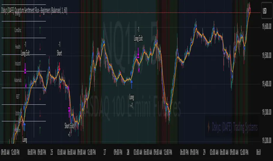
Dskyz (DAFE) Quantum Sentiment Flux - Beginners Dskyz (DAFE) Quantum Sentiment Flux - Beginners:
Welcome to the Dskyz (DAFE) Quantum Sentiment Flux - Beginners , a strategy and concept that’s your ultimate wingman for trading futures like MNQ, NQ, MES, and ES. This gem combines lightning-fast momentum signals, market sentiment smarts, and bulletproof risk management into a system so intuitive, even newbies can trade like pros. With clean DAFE visuals, preset modes for every vibe, and a revamped dashboard that’s basically a market GPS, this strategy makes futures trading feel like a high-octane sci-fi mission.
Built on the Dskyz (DAFE) legacy of Aurora Divergence, the Quantum Sentiment Flux is designed to empower beginners while giving seasoned traders a lean, sentiment-driven edge. It uses fast/slow EMA crossovers for entries, filters trades with VIX, SPX trends, and sector breadth, and keeps your account safe with adaptive stops and cooldowns. Tuned for more action with faster signals and a slick bottom-left dashboard, this updated version is ready to light up your charts and outsmart institutional traps. Let’s dive into why this strat’s a must-have and break down its brilliance.
Why Traders Need This Strategy
Futures markets are a wild ride—fast moves, volatility spikes (like the April 28, 2025 NQ 1k-point drop), and institutional games that can wreck unprepared traders. Beginners often get lost in complex systems or burned by impulsive trades. The Quantum Sentiment Flux is the antidote, offering:
Dead-Simple Setup: Preset modes (Aggressive, Balanced, Conservative) auto-tune signals, risk, and sizing, so you can trade without a quant degree.
Sentiment Superpower: VIX filter, SPX trend, and sector breadth visuals keep you aligned with market health, dodging chop and riding trends.
Ironclad Safety: Tighter ATR-based stops, 2:1 take-profits, and preset cooldowns protect your capital, even in chaotic sessions.
Next-Level Visuals: Green/red entry triangles, vibrant EMAs, a sector breadth background, and a beefed-up dashboard make signals and context pop.
DAFE Swagger: The clean aesthetics, sleek dashboard—ties it to Dskyz’s elite brand, making your charts a work of art.
Traders need this because it’s a plug-and-play system that blends beginner-friendly simplicity with pro-level market awareness. Whether you’re just starting or scalping 5min MNQ, this strat’s your key to trading with confidence and style.
Strategy Components
1. Core Signal Logic (High-Speed Momentum)
The strategy’s engine is a momentum-based system using fast and slow Exponential Moving Averages (EMAs), now tuned for faster, more frequent trades.
How It Works:
Fast/Slow EMAs: Fast EMA (Aggressive: 5, Balanced: 7, Conservative: 9 bars) and slow EMA (12/14/18 bars) track short-term vs. longer-term momentum.
Crossover Signals:
Buy: Fast EMA crosses above slow EMA, and trend_dir = 1 (fast EMA > slow EMA + ATR * strength threshold).
Sell: Fast EMA crosses below slow EMA, and trend_dir = -1 (fast EMA < slow EMA - ATR * strength threshold).
Strength Filter: ma_strength = fast EMA - slow EMA must exceed an ATR-scaled threshold (Aggressive: 0.15, Balanced: 0.18, Conservative: 0.25) for robust signals.
Trend Direction: trend_dir confirms momentum, filtering out weak crossovers in choppy markets.
Evolution:
Faster EMAs (down from 7–10/21–50) catch short-term trends, perfect for active futures markets.
Lower strength thresholds (0.15–0.25 vs. 0.3–0.5) make signals more sensitive, boosting trade frequency without sacrificing quality.
Preset tuning ensures beginners get optimized settings, while pros can tweak via mode selection.
2. Market Sentiment Filters
The strategy leans hard into market sentiment with a VIX filter, SPX trend analysis, and sector breadth visuals, keeping trades aligned with the big picture.
VIX Filter:
Logic: Blocks long entries if VIX > threshold (default: 20, can_long = vix_close < vix_limit). Shorts are always allowed (can_short = true).
Impact: Prevents longs during high-fear markets (e.g., VIX spikes in crashes), while allowing shorts to capitalize on downturns.
SPX Trend Filter:
Logic: Compares S&P 500 (SPX) close to its SMA (Aggressive: 5, Balanced: 8, Conservative: 12 bars). spx_trend = 1 (UP) if close > SMA, -1 (DOWN) if < SMA, 0 (FLAT) if neutral.
Impact: Provides dashboard context, encouraging trades that align with market direction (e.g., longs in UP trend).
Sector Breadth (Visual):
Logic: Tracks 10 sector ETFs (XLK, XLF, XLE, etc.) vs. their SMAs (same lengths as SPX). Each sector scores +1 (bullish), -1 (bearish), or 0 (neutral), summed as breadth (-10 to +10).
Display: Green background if breadth > 4, red if breadth < -4, else neutral. Dashboard shows sector trends (↑/↓/-).
Impact: Faster SMA lengths make breadth more responsive, reflecting sector rotations (e.g., tech surging, energy lagging).
Why It’s Brilliant:
- VIX filter adds pro-level volatility awareness, saving beginners from panic-driven losses.
- SPX and sector breadth give a 360° view of market health, boosting signal confidence (e.g., green BG + buy signal = high-probability trade).
- Shorter SMAs make sentiment visuals react faster, perfect for 5min charts.
3. Risk Management
The risk controls are a fortress, now tighter and more dynamic to support frequent trading while keeping accounts safe.
Preset-Based Risk:
Aggressive: Fast EMAs (5/12), tight stops (1.1x ATR), 1-bar cooldown. High trade frequency, higher risk.
Balanced: EMAs (7/14), 1.2x ATR stops, 1-bar cooldown. Versatile for most traders.
Conservative: EMAs (9/18), 1.3x ATR stops, 2-bar cooldown. Safer, fewer trades.
Impact: Auto-scales risk to match style, making it foolproof for beginners.
Adaptive Stops and Take-Profits:
Logic: Stops = entry ± ATR * atr_mult (1.1–1.3x, down from 1.2–2.0x). Take-profits = entry ± ATR * take_mult (2x stop distance, 2:1 reward/risk). Longs: stop below entry, TP above; shorts: vice versa.
Impact: Tighter stops increase trade turnover while maintaining solid risk/reward, adapting to volatility.
Trade Cooldown:
Logic: Preset-driven (Aggressive/Balanced: 1 bar, Conservative: 2 bars vs. old user-input 2). Ensures bar_index - last_trade_bar >= cooldown.
Impact: Faster cooldowns (especially Aggressive/Balanced) allow more trades, balanced by VIX and strength filters.
Contract Sizing:
Logic: User sets contracts (default: 1, max: 10), no preset cap (unlike old 7/5/3 suggestion).
Impact: Flexible but risks over-leverage; beginners should stick to low contracts.
Built To Be Reliable and Consistent:
- Tighter stops and faster cooldowns make it a high-octane system without blowing up accounts.
- Preset-driven risk removes guesswork, letting newbies trade confidently.
- 2:1 TPs ensure profitable trades outweigh losses, even in volatile sessions like April 27, 2025 ES slippage.
4. Trade Entry and Exit Logic
The entry/exit rules are simple yet razor-sharp, now with VIX filtering and faster signals:
Entry Conditions:
Long Entry: buy_signal (fast EMA crosses above slow EMA, trend_dir = 1), no position (strategy.position_size = 0), cooldown passed (can_trade), and VIX < 20 (can_long). Enters with user-defined contracts.
Short Entry: sell_signal (fast EMA crosses below slow EMA, trend_dir = -1), no position, cooldown passed, can_short (always true).
Logic: Tracks last_entry_bar for visuals, last_trade_bar for cooldowns.
Exit Conditions:
Stop-Loss/Take-Profit: ATR-based stops (1.1–1.3x) and TPs (2x stop distance). Longs exit if price hits stop (below) or TP (above); shorts vice versa.
No Other Exits: Keeps it straightforward, relying on stops/TPs.
5. DAFE Visuals
The visuals are pure DAFE magic, blending clean function with informative metrics utilized by professionals, now enhanced by faster signals and a responsive breadth background:
EMA Plots:
Display: Fast EMA (blue, 2px), slow EMA (orange, 2px), using faster lengths (5–9/12–18).
Purpose: Highlights momentum shifts, with crossovers signaling entries.
Sector Breadth Background:
Display: Green (90% transparent) if breadth > 4, red (90%) if breadth < -4, else neutral.
Purpose: Faster breadth_sma_len (5–12 vs. 10–50) reflects sector shifts in real-time, reinforcing signal strength.
- Visuals are intuitive, turning complex signals into clear buy/sell cues.
- Faster breadth background reacts to market rotations (e.g., tech vs. energy), giving a pro-level edge.
6. Sector Breadth Dashboard
The new bottom-left dashboard is a game-changer, a 3x16 table (black/gray theme) that’s your market command center:
Metrics:
VIX: Current VIX (red if > 20, gray if not).
SPX: Trend as “UP” (green), “DOWN” (red), or “FLAT” (gray).
Trade Longs: “OK” (green) if VIX < 20, “BLOCK” (red) if not.
Sector Breadth: 10 sectors (Tech, Financial, etc.) with trend arrows (↑ green, ↓ red, - gray).
Placeholder Row: Empty for future metrics (e.g., ATR, breadth score).
Purpose: Consolidates regime, volatility, market trend, and sector data, making decisions a breeze.
- VIX and SPX metrics add context, helping beginners avoid bad trades (e.g., no longs if “BLOCK”).
Sector arrows show market health at a glance, like a cheat code for sentiment.
Key Features
Beginner-Ready: Preset modes and clear visuals make futures trading a breeze.
Sentiment-Driven: VIX filter, SPX trend, and sector breadth keep you in sync with the market.
High-Frequency: Faster EMAs, tighter stops, and short cooldowns boost trade volume.
Safe and Smart: Adaptive stops/TPs and cooldowns protect capital while maximizing wins.
Visual Mastery: DAFE’s clean flair, EMAs, dashboard—makes trading fun and clear.
Backtestable: Lean code and fixed qty ensure accurate historical testing.
How to Use
Add to Chart: Load on a 5min MNQ/ES chart in TradingView.
Pick Preset: Aggressive (scalping), Balanced (versatile), or Conservative (safe). Balanced is default.
Set Contracts: Default 1, max 10. Stick low for safety.
Check Dashboard: Bottom-left shows preset, VIX, SPX, and sectors. “OK” + green breadth = strong buy.
Backtest: Run in strategy tester to compare modes.
Live Trade: Connect to Tradovate or similar. Watch for slippage (e.g., April 27, 2025 ES issues).
Replay Test: Try April 28, 2025 NQ drop to see VIX filter and stops in action.
Why It’s Brilliant
The Dskyz (DAFE) Quantum Sentiment Flux - Beginners is a masterpiece of simplicity and power. It takes pro-level tools—momentum, VIX, sector breadth—and wraps them in a system anyone can run. Faster signals and tighter stops make it a trading machine, while the VIX filter and dashboard keep you ahead of market chaos. The DAFE visuals and bottom-left command center turn your chart into a futuristic cockpit, guiding you through every trade. For beginners, it’s a safe entry to futures; for pros, it’s a scalping beast with sentiment smarts. This strat doesn’t just trade—it transforms how you see the market.
Final Notes
This is more than a strategy—it’s your launchpad to mastering futures with Dskyz (DAFE) flair. The Quantum Sentiment Flux blends accessibility, speed, and market savvy to help you outsmart the game. Load it, watch those triangles glow, and let’s make the markets your canvas!
Official Statement from Pine Script Team
(see TradingView help docs and forums):
"This warning may appear when you call functions such as ta.sma inside a request.security in a loop. There is no runtime impact. If you need to loop through a dynamic list of tickers, this cannot be avoided in the present version... Values will still be correct. Ignore this warning in such contexts."
(This publishing will most likely be taken down do to some miscellaneous rule about properly displaying charting symbols, or whatever. Once I've identified what part of the publishing they want to pick on, I'll adjust and repost.)
Use it with discipline. Use it with clarity. Trade smarter.
**I will continue to release incredible strategies and indicators until I turn this into a brand or until someone offers me a contract.
Created by Dskyz, powered by DAFE Trading Systems. Trade fast, trade bold.
Cerca negli script per "Futures"
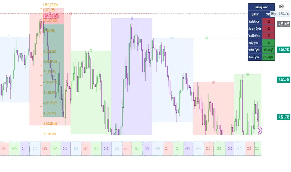
Quarterly Cycle Theory with DST time AdjustedThe Quarterly Theory removes ambiguity, as it gives specific time-based reference points to look for when entering trades. Before being able to apply this theory to trading, one must first understand that time is fractal:
Yearly Quarters = 4 quarters of three months each.
Monthly Quarters = 4 quarters of one week each.
Weekly Quarters = 4 quarters of one day each (Monday - Thursday). Friday has its own specific function.
Daily Quarters = 4 quarters of 6 hours each = 4 trading sessions of a trading day.
Sessions Quarters = 4 quarters of 90 minutes each.
90 Minute Quarters = 4 quarters of 22.5 minutes each.
Yearly Cycle: Analogously to financial quarters, the year is divided in four sections of three months each:
Q1 - January, February, March.
Q2 - April, May, June (True Open, April Open).
Q3 - July, August, September.
Q4 - October, November, December.
S&P 500 E-mini Futures (daily candles) — Monthly Cycle.
Monthly Cycle: Considering that we have four weeks in a month, we start the cycle on the first month’s Monday (regardless of the calendar Day):
Q1 - Week 1: first Monday of the month.
Q2 - Week 2: second Monday of the month (True Open, Daily Candle Open Price).
Q3 - Week 3: third Monday of the month.
Q4 - Week 4: fourth Monday of the month.
S&P 500 E-mini Futures (4 hour candles) — Weekly Cycle.
Weekly Cycle: Daye determined that although the trading week is composed by 5 trading days, we should ignore Friday, and the small portion of Sunday’s price action:
Q1 - Monday.
Q2 - Tuesday (True Open, Daily Candle Open Price).
Q3 - Wednesday.
Q4 - Thursday.
S&P 500 E-mini Futures (1 hour candles) — Daily Cycle.
Daily Cycle: The Day can be broken down into 6 hour quarters. These times roughly define the sessions of the trading day, reinforcing the theory’s validity:
Q1 - 18:00 - 00:00 Asia.
Q2 - 00:00 - 06:00 London (True Open).
Q3 - 06:00 - 12:00 NY AM.
Q4 - 12:00 - 18:00 NY PM.
S&P 500 E-mini Futures (15 minute candles) — 6 Hour Cycle.
6 Hour Quarters or 90 Minute Cycle / Sessions divided into four sections of 90 minutes each (EST/EDT):
Asian Session
Q1 - 18:00 - 19:30
Q2 - 19:30 - 21:00 (True Open)
Q3 - 21:00 - 22:30
Q4 - 22:30 - 00:00
London Session
Q1 - 00:00 - 01:30
Q2 - 01:30 - 03:00 (True Open)
Q3 - 03:00 - 04:30
Q4 - 04:30 - 06:00
NY AM Session
Q1 - 06:00 - 07:30
Q2 - 07:30 - 09:00 (True Open)
Q3 - 09:00 - 10:30
Q4 - 10:30 - 12:00
NY PM Session
Q1 - 12:00 - 13:30
Q2 - 13:30 - 15:00 (True Open)
Q3 - 15:00 - 16:30
Q4 - 16:30 - 18:00
S&P 500 E-mini Futures (5 minute candles) — 90 Minute Cycle.
Micro Cycles: Dividing the 90 Minute Cycle yields 22.5 Minute Quarters, also known as Micro Sessions or Micro Quarters:
Asian Session
Q1/1 18:00:00 - 18:22:30
Q2 18:22:30 - 18:45:00
Q3 18:45:00 - 19:07:30
Q4 19:07:30 - 19:30:00
Q2/1 19:30:00 - 19:52:30 (True Session Open)
Q2/2 19:52:30 - 20:15:00
Q2/3 20:15:00 - 20:37:30
Q2/4 20:37:30 - 21:00:00
Q3/1 21:00:00 - 21:23:30
etc. 21:23:30 - 21:45:00
London Session
00:00:00 - 00:22:30 (True Daily Open)
00:22:30 - 00:45:00
00:45:00 - 01:07:30
01:07:30 - 01:30:00
01:30:00 - 01:52:30 (True Session Open)
01:52:30 - 02:15:00
02:15:00 - 02:37:30
02:37:30 - 03:00:00
03:00:00 - 03:22:30
03:22:30 - 03:45:00
03:45:00 - 04:07:30
04:07:30 - 04:30:00
04:30:00 - 04:52:30
04:52:30 - 05:15:00
05:15:00 - 05:37:30
05:37:30 - 06:00:00
New York AM Session
06:00:00 - 06:22:30
06:22:30 - 06:45:00
06:45:00 - 07:07:30
07:07:30 - 07:30:00
07:30:00 - 07:52:30 (True Session Open)
07:52:30 - 08:15:00
08:15:00 - 08:37:30
08:37:30 - 09:00:00
09:00:00 - 09:22:30
09:22:30 - 09:45:00
09:45:00 - 10:07:30
10:07:30 - 10:30:00
10:30:00 - 10:52:30
10:52:30 - 11:15:00
11:15:00 - 11:37:30
11:37:30 - 12:00:00
New York PM Session
12:00:00 - 12:22:30
12:22:30 - 12:45:00
12:45:00 - 13:07:30
13:07:30 - 13:30:00
13:30:00 - 13:52:30 (True Session Open)
13:52:30 - 14:15:00
14:15:00 - 14:37:30
14:37:30 - 15:00:00
15:00:00 - 15:22:30
15:22:30 - 15:45:00
15:45:00 - 15:37:30
15:37:30 - 16:00:00
16:00:00 - 16:22:30
16:22:30 - 16:45:00
16:45:00 - 17:07:30
17:07:30 - 18:00:00
S&P 500 E-mini Futures (30 second candles) — 22.5 Minute Cycle.
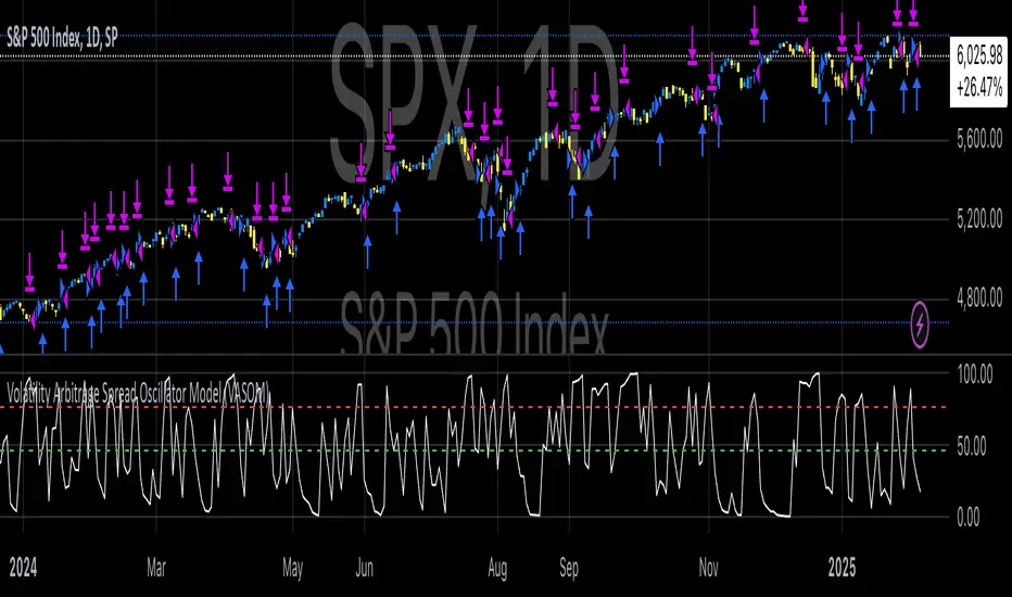
Volatility Arbitrage Spread Oscillator Model (VASOM)The Volatility Arbitrage Spread Oscillator Model (VASOM) is a systematic approach to capitalizing on price inefficiencies in the VIX futures term structure. By analyzing the differential between front-month and second-month VIX futures contracts, we employ a momentum-based oscillator (Relative Strength Index, RSI) to signal potential market reversion opportunities. Our research builds upon existing financial literature on volatility risk premia and contango/backwardation dynamics in the volatility markets (Zhang & Zhu, 2006; Alexander & Korovilas, 2012).
Volatility derivatives have become essential tools for managing risk and engaging in speculative trades (Whaley, 2009). The Chicago Board Options Exchange (CBOE) Volatility Index (VIX) measures the market’s expectation of 30-day forward-looking volatility derived from S&P 500 option prices (CBOE, 2018). Term structures in VIX futures often exhibit contango or backwardation, depending on macroeconomic and market conditions (Alexander & Korovilas, 2012).
This strategy seeks to exploit the spread between the front-month and second-month VIX futures as a proxy for term structure dynamics. The spread’s momentum, quantified by the RSI, serves as a signal for entry and exit points, aligning with empirical findings on mean reversion in volatility markets (Zhang & Zhu, 2006).
• Entry Signal: When RSI_t falls below the user-defined threshold (e.g., 30), indicating a potential undervaluation in the spread.
• Exit Signal: When RSI_t exceeds a threshold (e.g., 70), suggesting mean reversion has occurred.
Empirical Justification
The strategy aligns with findings that suggest predictable patterns in volatility futures spreads (Alexander & Korovilas, 2012). Furthermore, the use of RSI leverages insights from momentum-based trading models, which have demonstrated efficacy in various asset classes, including commodities and derivatives (Jegadeesh & Titman, 1993).
References
• Alexander, C., & Korovilas, D. (2012). The Hazards of Volatility Investing. Journal of Alternative Investments, 15(2), 92-104.
• CBOE. (2018). The VIX White Paper. Chicago Board Options Exchange.
• Jegadeesh, N., & Titman, S. (1993). Returns to Buying Winners and Selling Losers: Implications for Stock Market Efficiency. The Journal of Finance, 48(1), 65-91.
• Zhang, C., & Zhu, Y. (2006). Exploiting Predictability in Volatility Futures Spreads. Financial Analysts Journal, 62(6), 62-72.
• Whaley, R. E. (2009). Understanding the VIX. The Journal of Portfolio Management, 35(3), 98-105.
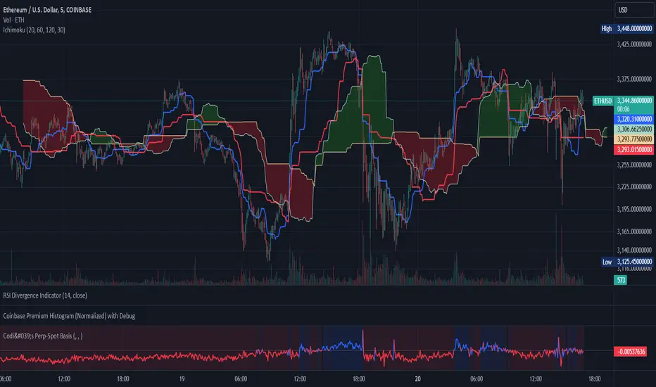
Codi's Perp-Spot Basis# Perp-Spot Basis Indicator
This indicator calculates the percentage basis between perpetual futures and spot prices for crypto assets. It is inspired by the original concept from **Krugermacro**, with the added improvement of **automatic detection of the asset pairs** based on the current chart symbol. This enhancement makes it faster and easier to apply across different assets without manual configuration.
## How It Works
The indicator compares the perpetual futures price (e.g., `BTCUSDT.P`) to the spot price (e.g., `BTCUSDT`) on Binance. The difference is expressed as a percentage: (Perp - Spot) / Spot * 100
The results are displayed in a color-coded graph:
- **Blue (Positive Basis):** Perpetual futures are trading at a premium, indicating **bullish sentiment** among derivatives traders.
- **Red (Negative Basis):** Perpetual futures are trading at a discount, indicating **bearish sentiment** among derivatives traders.
This percentage basis is a core component in understanding funding rates and derivatives market dynamics. It serves as a faster proxy for funding rates, which typically lag behind real-time price movements.
---
## How to Use It
### General Concept
- **Red (Negative Basis):** Ideal to execute **longs** when derivatives traders are overly bearish.
- **Blue (Positive Basis):** Ideal to execute **shorts** when derivatives traders are overly bullish.
### Pullback Sniping
1. During an **uptrend**:
- If the basis turns **red** temporarily, it can signal an opportunity to **buy the dip**.
2. During a **downtrend**:
- If the basis turns **blue** temporarily, it can signal an opportunity to **sell the rip**.
3. Wait for the basis to **pop back** (higher in uptrend, lower in downtrend) to time entries more effectively—this often coincides with **stop runs** or **liquidations**.
### Intraday Execution
- **When price is falling**:
- If the basis is **red**, the move is derivatives-led (**normal**).
- If the basis is **blue**, spot traders are leading, and perps are offside—wait for **price dumps** before longing.
- **When price is rising**:
- If the basis is **blue**, the move is derivatives-led (**normal**).
- If the basis is **red**, spot traders are leading, and perps are offside—wait for **price pops** before shorting.
### Larger Time Frames
- **Consistently Blue Basis:** Indicates a **bull market** as derivatives traders are bullish over the long term.
- **Consistently Red Basis:** Indicates a **bear market** as derivatives traders are bearish over the long term.
---
## Improvements Over the Original
This version of the Perp-Spot Basis indicator **automatically detects the Binance perpetual futures and spot pairs** based on the current chart symbol. For example:
- If you are viewing `ETHUSDT`, it automatically references `ETHUSDT.P` for the perpetual futures pair and `ETHUSDT` for the spot pair in BINANCE.
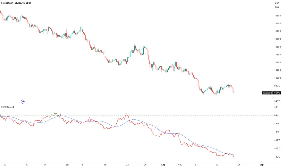
FCNC SpreadTitle: FCNC Spread Indicator
Description:
The FCNC Spread Indicator is designed to help traders analyze the price difference (spread) between two futures contracts: the front contract and the next contract. This type of analysis is commonly used in futures trading to identify market sentiment, arbitrage opportunities, and potential roll yield strategies.
How It Works:
Front Contract: The front contract represents the futures contract closest to expiration, often referred to as the near-month contract.
Next Contract: The next contract is the futures contract that follows the front contract in the expiration cycle, typically the next available month.
Spread Calculation: frontContract - nextContract represents the difference between the price of the front contract and the next contract.
Positive Spread: A positive value means that the front contract is more expensive than the next contract, indicating backwardation.
Negative Spread: A negative value means that the front contract is cheaper than the next contract, indicating contango.
How to Use:
Input Selection: Select your desired futures contracts for the front and next contract through the input settings. The script will fetch and calculate the closing prices of these contracts.
Spread Plotting: The calculated spread is plotted on the chart, with color-coding based on the spread's value (green for positive, red for negative).
Labeling: The spread value is dynamically labeled on the chart for quick reference.
Moving Average: A 20-period Simple Moving Average (SMA) of the spread is also plotted to help identify trends and smooth out fluctuations.
Applications:
Trend Identification: Analyze the spread to determine market sentiment and potential trend reversals.
Divergence Detection: Look for divergences between the spread and the underlying market to identify possible shifts in trend or market sentiment. Divergences can signal upcoming reversals or provide early warning signs of a change in market dynamics.
This indicator is particularly useful for futures traders who are looking to gain insights into the market structure and to exploit differences in contract pricing. By providing a clear visualization of the spread between two key futures contracts, traders can make more informed decisions about their trading strategies.
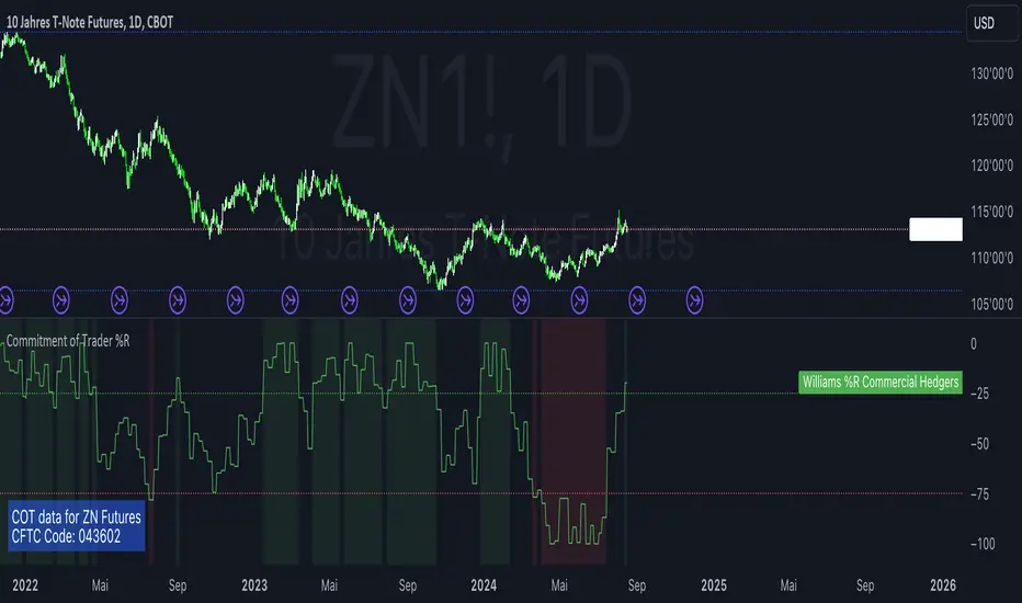
Commitment of Trader %RThis script is a TradingView Pine Script that creates a custom indicator to analyze Commitment of Traders (COT) data. It leverages the TradingView COT library to fetch data related to futures and options markets, processes this data, and then applies the Williams %R indicator to the COT data to assist in trading decisions. Here’s a detailed explanation of its components and functionality:
Importing and Configuration:
The script imports the COT library from TradingView and sets up tooltips to explain different input options to the user.
It allows the user to choose the mode for fetching COT data, which can be based on the root of the symbol, base currency, or quote currency.
Users can also input a specific CFTC code directly, instead of relying on automatic code generation.
Inputs and Parameters:
The script provides inputs to select the type of data (futures, options, or both), the type of COT data to display (long positions, short positions, etc.), and thresholds for the Williams %R indicator.
It also allows setting the period for the Williams %R calculation.
Data Request and Processing:
The dataRequest function fetches COT data for large traders, small traders, and commercial hedgers.
The script calculates the Williams %R for each type of trader, which measures overbought and oversold conditions.
Visualization:
The script uses background colors to highlight when the Williams %R crosses the specified thresholds for commercial hedgers.
It plots the COT data and Williams %R on the chart, with different colors representing large traders, small traders, and commercial hedgers.
Horizontal lines are drawn to indicate the upper and lower thresholds.
Display Information:
A table is displayed on the chart’s lower left corner showing the current COT data and CFTC code used.
Use of COT Report in Futures Trading
The COT report is a weekly publication by the Commodity Futures Trading Commission (CFTC) that provides insights into the positions held by different types of traders in the futures markets. This information is valuable for traders as it shows:
Market Sentiment: By analyzing the positions of commercial traders (often considered to be more informed), non-commercial traders (speculative traders), and small traders, traders can gauge market sentiment and potential future movements.
Contrarian Indicators: Large shifts in positions, especially when non-commercial traders hold extreme positions, can signal potential reversals or trends.
Research on COT Data and Price Movements
Several academic studies have examined the relationship between COT data and price movements in financial markets. Here are a few key works:
"The Predictive Power of the Commitment of Traders Report" by Jacob J. (2009):
This paper explores how changes in the positions of different types of traders in the COT report can predict future price movements in futures markets.
Citation: Jacob, J. (2009). The Predictive Power of the Commitment of Traders Report. Journal of Futures Markets.
"A New Look at the Commitment of Traders Report" by Mitchell, C. (2010):
Mitchell analyzes the efficacy of using COT data as a trading signal and its impact on trading strategies.
Citation: Mitchell, C. (2010). A New Look at the Commitment of Traders Report. Financial Analysts Journal.
"Market Timing Using the Commitment of Traders Report" by Kirkpatrick, C., & Dahlquist, J. (2011):
This study investigates the use of COT data for market timing and the effectiveness of various trading strategies based on the report.
Citation: Kirkpatrick, C., & Dahlquist, J. (2011). Market Timing Using the Commitment of Traders Report. Technical Analysis of Stocks & Commodities.
These studies provide insights into how COT data can be utilized for forecasting and trading decisions, reinforcing the utility of incorporating such data into trading strategies.
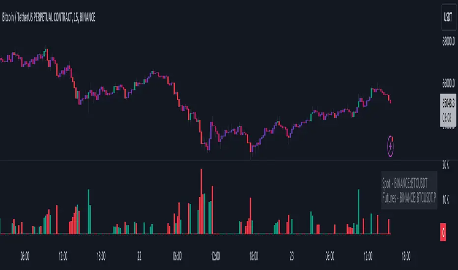
Volume Liqidations [EagleVSniper]The Volume Liquidations Indicator is designed for traders who want to spot significant liquidation events in the cryptocurrency markets, particularly between spot and futures volumes. This powerful tool auto-detects the trading asset and compares the volume data from both spot and futures markets to highlight potential high-volume liquidation points that can significantly impact price movement. Raw source code owner - tartigradia
Features:
Auto-Detect Functionality: Automatically identifies the current trading asset, providing an option for manual selection for both spot and futures symbols.
Volume Comparison: Calculates the difference between futures and spot volumes within a user-defined timeframe, helping to identify liquidation events.
Customizable Parameters: Offers customizable options for multipliers, lookback periods, and timeframe selection to tailor the indicator to your trading strategy.
Visual Indicators: Displays liquidation volumes as color-coded columns, with green indicating potential long liquidations and red for short liquidations. It also highlights bars that exceed the high-volume threshold, providing a clear visual cue for significant liquidation events.
Spot and Futures Volume MA: Includes optional moving average plots for both spot and futures volumes, allowing for a deeper analysis of market trends.
Highlighting High-Volatility Candles: The indicator uniquely colors candles that reach a predefined volatility threshold, determined by the user-set multiplier. This functionality aims to spotlight moments of significant market volatility, providing traders with immediate visual cues.
Dynamic Ticker Selection: Seamlessly switches between auto and manual ticker selection, providing flexibility for all types of traders.
How to Use:
Setup: Configure the indicator to your preferences. You can choose between automatic or manual ticker selection, set the multiplier for the high-volume threshold, and define the lookback period for the moving average calculation.
Analysis: The indicator plots differences in volume between futures and spot markets as columns on your chart, color-coded to indicate the direction of potential liquidations.
Decision Making: Use the indicator to identify potential liquidation events. High-volume thresholds are highlighted, suggesting significant market movements. Combine this information with other analysis tools to make informed trading decisions.
@tk · spectral█ OVERVIEW
This script is an indicator that helps traders to identify the price difference between spot and futures of the current crypto plotted into the chart. It works in both types of markets, when the chart is plotting the crypto in spot market, it will compare with its respective futures ticker and vice-versa. If the current asset isn't a crypt ticker, the indicator will not be plotted into the chart.
█ MOTIVATION
Since crypto's derivative market is based on spot market asset's price, to calculate the arbitrage mechanisms that attempts to balance the asset price, this indicator can help traders to identify some spot and futures price divergence that can create an anomaly of funding rate and can push it to an extreme negative — or positive — rate. So, easing to track the price difference between both markets will bring more evidences to identify an artificial price move, specially in crypto assets with low market cap.
█ CONCEPT
The trading concept to use this indicator is the concept of the arbitrage machamism created by exchanges that calculates the funding rate based on spot and futures price difference that will vary from exchange to exchange. This strategy don't works alone. It needs to be aligned together with others indicators like Exponential Moving Averages, Chart Patterns, Support and Resistance, and so on... Even more confluences that you have, bigger are your chances to increase the probability for a successful trade. So, don't use this indicator alone. Compose a trading strategy and use it to improve your analysis.
█ CUSTOMIZATION
This indicator allows the trader to customize the following settings:
GENERAL
Text size
Changes the font size of price difference table to improve accessibility.
Type: string
Options: `tiny`, `small`, `normal`, `large`.
Default: `small`
Position
Changes the position of price difference table.
Type: string
Options: `top_left`, `top_center`, `top_right`, `middle_left`, `middle_center`, `middle_right`, `bottom_left`, `bottom_center`, `bottom_right`.
Default: `bottom_right`
Pair Quote
The ticker quote symbol that will be used to base the ticker comparison from spot to futures (e.g. BTCUSDT which `USDT` is the quote. ETHBTC which `BTC` is the quote).
Type: string
Default: USDT
Spectrum Color
The color of the spectrum candles. Spectrum candles are the candles of the opposite market. If the current ticker is in the spot market, the spectrum candles will be the price of the futures market.
Type: color
Default: #434651
█ FUNCTIONS
The indicator contains the following functions:
stripStarts(src, str)
Strips a defined pattern from a string.
Parameters:
src: (string) Source string
str: (string) String pattern to be stripped from start of source string.
Returns: (string) Stripped string with matched regex pattern.

Open Interest Chart [LuxAlgo]The Open Interest Chart displays Commitments of Traders %change of futures open interest , with a unique circular plotting technique, inspired from this publication Periodic Ellipses .
🔶 USAGE
Open interest represents the total number of contracts that have been entered by market participants but have not yet been offset or delivered. This can be a direct indicator of market activity/liquidity, with higher open interest indicating a more active market.
Increasing open interest is highlighted in green on the circular plot, indicating money coming into the market, while decreasing open interests highlighted in red indicates money coming out of the market.
You can set up to 6 different Futures Open interest tickers for a quick follow up:
🔶 DETAILS
Circles are drawn, using plot() , with the functions createOuterCircle() (for the largest circle) and createInnerCircle() (for inner circles).
Following snippet will reload the chart, so the circles will remain at the right side of the chart:
if ta.change(chart.left_visible_bar_time ) or
ta.change(chart.right_visible_bar_time)
n := bar_index
Here is a snippet which will draw a 39-bars wide circle that will keep updating its position to the right.
//@version=5
indicator("")
n = bar_index
barsTillEnd = last_bar_index - n
if ta.change(chart.left_visible_bar_time ) or
ta.change(chart.right_visible_bar_time)
n := bar_index
createOuterCircle(radius) =>
var int end = na
var int start = na
var basis = 0.
barsFromNearestEdgeCircle = 0.
barsTillEndFromCircleStart = radius
startCylce = barsTillEnd % barsTillEndFromCircleStart == 0 // start circle
bars = ta.barssince(startCylce)
barsFromNearestEdgeCircle := barsTillEndFromCircleStart -1
basis := math.min(startCylce ? -1 : basis + 1 / barsFromNearestEdgeCircle * 2, 1) // 0 -> 1
shape = math.sqrt(1 - basis * basis)
rad = radius / 2
isOK = barsTillEnd <= barsTillEndFromCircleStart and barsTillEnd > 0
hi = isOK ? (rad + shape * radius) - rad : na
lo = isOK ? (rad - shape * radius) - rad : na
start := barsTillEnd == barsTillEndFromCircleStart ? n -1 : start
end := barsTillEnd == 0 ? start + radius : end
= createOuterCircle(40)
plot(h), plot(l)
🔶 LIMITATIONS
Due to the inability to draw between bars, from time to time, drawings can be slightly off.
Bar-replay can be demanding, since it has to reload on every bar progression. We don't recommend using this script on bar-replay. If you do, please choose the lowest speed and from time to time pause bar-replay for a second. You'll see the script gets reloaded.
🔶 SETTINGS
🔹 TICKERS
Toggle :
• Enabled -> uses the first column with a pre-filled list of Futures Open Interest tickers/symbols
• Disabled -> uses the empty field where you can enter your own ticker/symbol
Pre-filled list : the first column is filled with a list, so you can choose your open interest easily, otherwise you would see COT:088691_F_OI aka Gold Futures Open Interest for example.
If applicable, you will see 3 different COT data:
• COT: Legacy Commitments of Traders report data
• COT2: Disaggregated Commitments of Traders report data
• COT3: Traders in Financial Futures report data
Empty field : When needed, you can pick another ticker/symbol in the empty field at the right and disable the toggle.
Timeframe : Commitments of Traders (COT) data is tallied by the Commodity Futures Trading Commission (CFTC) and is published weekly. Therefore data won't change every day.
Default set TF is Daily
🔹 STYLE
From middle:
• Enabled (default): Drawings start from the middle circle -> towards outer circle is + %change , towards middle of the circle is - %change
• Disabled: Drawings start from the middle POINT of the circle, towards outer circle is + OR -
-> in both options, + %change will be coloured green , - %change will be coloured red .
-> 0 %change will be coloured blue , and when no data is available, this will be coloured gray .
Size circle : options tiny, small, normal, large, huge.
Angle : Only applicable if "From middle" is disabled!
-> sets the angle of the spike:
Show Ticker : Name of ticker, as seen in table, will be added to labels.
Text - fill
• Sets colour for +/- %change
Table
• Sets 2 text colours, size and position
Circles
• Sets the colour of circles, style can be changed in the Style section.
You can make it as crazy as you want:

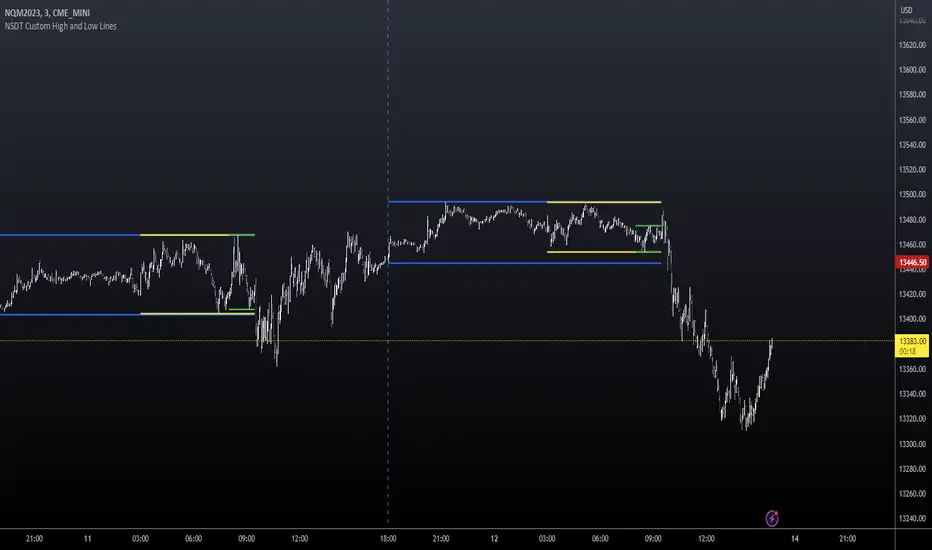
NSDT Custom High and Low LinesFirst, the credit for the original script to plot a High and Low between a certain time goes to developer paaax.
I took that idea, converted it to Pinescript V5, cleaned up the code, and added a few more lines so you can plot different levels based on time of day.
Published open source like the original.
The example shown has:
Blue - plotting from the start of the Futures Asian session to the start of the Futures USA Session. (6:00PM - 9:30AM Eastern)
Yellow - plotting from the start of the Futures Europe session to the start of the Futures USA Session. (3:00AM - 9:30AM Eastern)
Green - plotting from the start of the Futures US Premarket session to the start of the Futures USA Session. (8:00AM - 9:30AM Eastern)
These are great levels to use for breakouts and/or support and resistance.
Combine these levels with the 5 min Open Range levels, as you have some good trades.
Each of the three sessions have individual start and end times that can be modified by the trader, so you can easily mark off important areas for your style of trading.
MicroStrategy MetricsA script showing all the key MSTR metrics. I will update the script every time degen Saylor sells some more office furniture to buy BTC.
All based around valuing MSTR, aside from its BTC holdings. I.e. the true market cap = enterprise value - BTC holdings. Hence, you're left with the value of the software business + any premium/discount decided by investors.
From this we can derive:
- BTC Holdings % of enterprise value
- Correlation to BTC (in this case we use CME futures...may change this)
- Equivalent Share Price (true market cap divided by shares outstanding)
- P/E Ratio (equivalent share price divided by quarterly EPS estimates x 4)
- Price to FCF Ratio (true market cap divided by FCF (ttm))
- Price to Revenue (^ but with total revenue (ttm))

Open Interest Auto SpaceManBTCOpen Interest Auto SpaceManBTC
This is an extension to the script, it aims to provide the data in a less hands on way by providing the basis for automatic calculation on which symbol the data is being pulled from.
Changelog:
Automatic Data retrieval on a percoin basis.
Ability to hide or show symbol.
Coloring choices for the user.

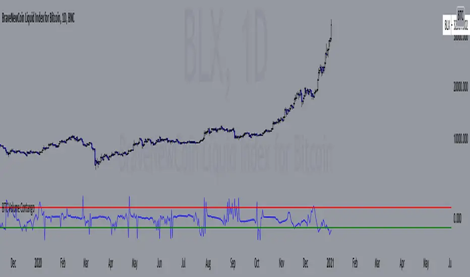
BTC Volume Contango IndexBased on my previous script "BTC Contango Index" which was inspired by a Twitter post by Byzantine General:
This is a script that shows the contango between spot and futures volumes of Bitcoin to identify overbought and oversold conditions. When a market is in contango, the volume of a futures contract is higher than the spot volume. Conversely, when a market is in backwardation, the volume of the futures contract is lower than the spot volume.
The aggregate daily volumes on top exchanges are taken to obtain Total Spot Volume and Total Futures Volume. The script then plots (Total Futures Volume/Total Spot Volume) - 1 to illustrate the percent difference (contango) between spot and futures volumes of Bitcoin. This data by itself is useful, but because aggregate futures volumes are so much larger than spot volumes, no negative values are produced. To correct for this, the Z-score of contango is taken. The Z-score (z) of a data item x measures the distance (in standard deviations StdDev) and direction of the item from its mean (U):
Z-score = (x - U) / StDev
A value of zero indicates that the data item x is equal to the mean U, while positive or negative values show that the data item is above or below the mean (x Values of +2 and -2 show that the data item is two standard deviations above or below the chosen mean, respectively, and over 95.5% of all data items are contained within these two horizontal references). We substitute x with volume contango C, the mean U with simple moving average ( SMA ) of n periods (50), and StdDev with the standard deviation of closing contango for n periods (50), so the above formula becomes: Z-score = (C - SMA (50)) / StdDev(C,50).
When in contango, Bitcoin may be overbought.
When in backwardation, Bitcoin may be oversold.
The current bar calculation will always look incorrect due to TV plotting the Z-score before the bar closes.
BTC Contango IndexInspired by a Twitter post by Byzantine General:
This is a script that shows the contango between spot and futures prices of Bitcoin to identify overbought and oversold conditions. Contango and backwardation are terms used to define the structure of the forward curve. When a market is in contango, the forward price of a futures contract is higher than the spot price. Conversely, when a market is in backwardation, the forward price of the futures contract is lower than the spot price.
The aggregate prices on top exchanges are taken and then averaged to obtain a Spot Average and a Futures Average. The script then plots (Futures Average/Spot Average) - 1 to illustrate the percent difference (contango) between spot and futures prices of Bitcoin.
When in contango, Bitcoin may be overbought.
When in backwardation, Bitcoin may be oversold.

Weis Pip Wave jayyWhat you see here is the Weis pip wave. The Weis pip wave shows how far in price a Weis wave has traveled through the duration of a Weis wave. The Weis pip wave is used in combination with the Weis cumulative volume wave. The two waves must be set to the same "wave size" and using the same method as described by Weis.
Using the traditional Weis method simply enter the desired wave size in the box "Select Weis Wave Size". In the example shown, it is set to 5 points. Each wave for each security and each timeframe requires its own wave size. Although not the traditional method a more automatic way to set wave size would be to use ATR. This is not the true Weis method but it does give you similar waves and, importantly, without the hassle of selecting a wave size for every chart. Once the Weis wave size is set then the pip wave will be shown.
I have put a zigzag of a 5 point Weis wave on the above bar chart. I have added it to allow your eye to get a better appreciation for Weis wave pivot points. You will notice that the wave is not in straight lines connecting wave tops to bottoms this is a function of the limitations of Pinescript version 1. This script would need to be in version 4 to allow straight lines. I will elaborate on the Weis pip zigzag script.
What is a Weis wave? David Weis has been recognized as a Wyckoff method analyst he has written two books one of which, Trades About to Happen, describes the evolution of the now popular Weis wave. The method employed by Weis is to identify waves of price action and to compare the strength of the waves on characteristics of wave strength. Chief among the characteristics of strength is the cumulative volume of the wave. There are other markers that Weis uses as well for example how the actual price difference between the start of the Weis wave from start to finish. Weis also uses time, particularly when using a Renko chart. Weis specifically uses candle/bar closes to define all wave action.
David Weis did a futures.io video which is a popular source of information about his method.
Cheers jayy
PS This script was published a day ago, however, I had included some links to the website of a person that uses Weis pip waves and also a dropbox link that contains the Weis wave chart for May 27, 2020, published by David Weis. Providing those links is against TV policy and so the script was hidden by TV. This is the identical script with the identical settings but without the offending links. If you want to see the pip Weis method in practice then search Weis pip wave. I have absolutely no affiliation. If you want to see Weis chart in pdf then message me and I will give a link or the Weis pdf. Why would you want to see the Weis chart for May 27, 2020? Merely to confirm the veracity of my algorithm. You could compare my chart () from the same period to the Weis chart. Both waves are for the ES!1 4 hour chart and both for a wave size of 5.

ADX Volatility Moving AverageThe ADXVMA is a volatility based moving average with the volatility being determined by the value of the ADX. The ADXVMA provides levels of support during uptrends and resistance during downtrends. Original NT indicator by Fat Tails on futures.io, just ported it to pinescript

Fibonacci BandsCreates bands based on Fibonacci numbers and the SMA.
Based on indicator by Big Mike on futures.io
How to trade
- Best to use in ranging market conditions
- Place on two different time frames eg. 15 and 55 min.
- Take trades off either short or long term chart.
- Best trades occur when both charts show same trigger/condition.
- Trades are short term reversals in direction of major trend on longer term chart unless you expect a trend reversal.
- Determine which band is the limiting band for the volatility of the instrument.
- When the market closes outside of the limiting band then returns inside, take a long/short one tick above/below the high/low of the previous bar.
- Place stop below/above the low/high of the the recent swing low/high.
- Set targets at opposite band of chart
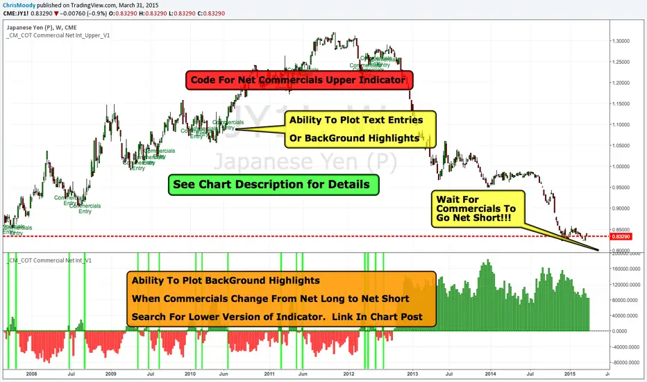
_CM_COT Commercial Net Interest_Upper_V1Overview.
-This is the Beginning of a Educational Series from Jake Bernstein to the TradingView Community.
-Many Traders use the COT Data Incorrectly.
-Jake Discovered if You Look at the Net Commercials and Take Note When Commercials net Buying is Either At All Time Highs, Or Net Buying = Longest Period of Buying Look for an Extreme Move To the Upside.
-In The Future We Will Show Precise Entry Signals…But a Basic Entry Signal Is When Commercials Go From Net Long to Net Short.
-Full Credit in Methodology goes to Jake Bernstein at www.Trade-Futures.com and www.2Chimps.net
Thought Process:
-Commercials Represent Large (Typically Billion Dollar) Companies.
-Take Note - When Commercials Are Buying at Record High
-Take Note - When Commercials Are Buying For Record Long Periods of Time
***Note…Commercials Can Buy For Extended Periods Dollar Cost Averaging…
***Basic Entry Listed In Overview.
***More Precise Entries Will Be Introduced Soon.
Indicator Shows Net Commercials
-Full Credit goes to Greeny for Creating Original Code. I only made slight modifications.
Modifications include
-Added Ability to Plot Text Entries when Commercials Switch From Net Long To Short
-Added Optional Background Highlighting when Commercials Switch from Long to Short
-Added Optional Alert Capability If Commercials Go From Net Long to Short
***Additional Indicators and Updates Coming Soon
***Link To Lower Indicator:
_CM_COT Commercial Net Interest_V1Overview.
-This is the Beginning of a Educational Series from Jake Bernstein to the TradingView Community.
-Many Traders use the COT Data Incorrectly.
-Jake Discovered if You Look at the Net Commercials and Take Note When Commercials net Buying is Either At All Time Highs, Or Net Buying = Longest Period of Buying Look for an Extreme Move To the Upside.
-In The Future We Will Show Precise Entry Signals…But a Basic Entry Signal Is When Commercials Go From Net Long to Net Short.
-Full Credit in Methodology goes to Jake Bernstein at www.Trade-Futures.com and www.2Chimps.net
Thought Process:
-Commercials Represent Large (Typically Billion Dollar) Companies.
-Take Note - When Commercials Are Buying at Record High
-Take Note - When Commercials Are Buying For Record Long Periods of Time
***Note…Commercials Can Buy For Extended Periods Dollar Cost Averaging…
***Basic Entry Listed In Overview.
***More Precise Entries Will Be Introduced Soon.
Indicator Shows Net Commercials
-Full Credit goes to Greeny for Creating Original Code. I only made slight modifications.
Modifications include
-Took Off Net Long and Short Individual Plots
-Added Optional Background Highlighting when Commercials Switch from Long to Short
-Added Optional Alert Capability If Commercials Go From Net Long to Short
-Ability to Show INVERSE - This makes it Easier for some Traders to See…Since the Signals look similar to MacD/RSI Type Indicators.
***Additional Indicators and Updates Coming Soon
***Link To Upper Indicator:

VX Term StructureThe VX Term Structure Monitor is an advanced visualization tool designed specifically for volatility traders who need to instantly recognize shifts in market structure. By comparing the current VIX Futures Term Structure against the previous trading day's close, this indicator provides a clear, real-time* view of the VIX Spot Index and the next available VX futures contracts. A key visual feature is the "Daily Drift" analysis, which automatically highlights the difference between today's curve (Cyan) and yesterday's curve (Gray/Dashed) with red or green fills, allowing you to immediately spot whether volatility is rising or falling across the term structure.
Unlike standard indicators that rely solely on the Spot price, this script utilizes professional-grade logic to classify market stress into three distinct stages. It identifies a normal Contango environment (Green) when the Front Month (M1) is trading below the Second Month (M2), indicating a calm market where long volatility positions typically suffer from negative roll yield. The system issues a Spot Warning (Orange) if the Spot index overheats and exceeds M1 while the futures curve remains in Contango, often an early signal of building stress. Finally, it detects critical Backwardation (Red) when the futures curve physically inverts (M1 > M2), signaling that market participants are paying a premium for immediate protection.
Usage Note: Due to technical limitations in detecting contract expirations automatically, users must manually select the current "Front Month" contract (e.g., "G (Feb)") in the indicator settings to ensure correct alignment. Users can also configure server-side alerts to trigger specifically when the market flips into Backwardation.
*Note: To view real-time data for VX futures, a paid data subscription to CBOE (CFE) is required on TradingView. Otherwise, the data may be delayed.
Disclaimer: This tool is for educational and informational purposes only and does not constitute financial advice.

NQ-Market Momentum CompassNQ-Market Momentum Compass: User Guide
Overview
NQ-Market Momentum Compass is a comparative momentum tool that helps you visualize the relative strength between Nasdaq futures (NQ) and a volume-weighted composite of other major US index futures (ES, RTY, and YM). This indicator plots two oscillator lines that move above and below zero, making it easy to identify momentum shifts and potential divergences between tech-heavy Nasdaq and the broader market.
What You're Looking At
The indicator displays two main components:
NQ Oscillator (Blue Line): Shows the percentage change in NQ futures over your selected lookback period.
Composite Oscillator (Orange Line): Shows the volume-weighted average percentage change of S&P 500 (ES), Russell 2000 (RTY), and Dow Jones (YM) futures over the same period.
Zero Line (Gray): The center reference line dividing positive and negative momentum.
How It Works
Core Calculation
The indicator calculates percentage change over a lookback period:
For each index, it computes: (current_price - price_n_bars_ago) / price_n_bars_ago * 100
The NQ line shows this calculation for Nasdaq futures
The composite line weights the other indices by their relative trading volumes
Volume Weighting
Instead of a simple average, the composite line incorporates trading volume to give more weight to indices with higher participation. This provides a more accurate representation of overall market momentum.
How to Interpret the Indicator
Basic Interpretation
Above Zero: Price is higher than it was at the lookback period ago (positive momentum)
Below Zero: Price is lower than it was at the lookback period ago (negative momentum)
Steepness: Indicates the strength of the momentum (steeper = stronger momentum)
Comparative Analysis
When Lines Move Together: NQ is moving in harmony with the broader market
When Lines Diverge:
NQ above composite: Tech/growth is outperforming the broader market
Composite above NQ: Broader market is outperforming tech/growth
Key Signals to Watch
Crossovers Between Lines: Potential shift in sector leadership
NQ crossing above composite: Tech starting to outperform
NQ crossing below composite: Tech starting to underperform
Zero-Line Crossovers: Change in overall momentum direction
Crossing above zero: Shift to positive momentum
Crossing below zero: Shift to negative momentum
Divergences: When one line makes a new high/low while the other doesn't, suggesting potential reversal
Practical Applications
Market Rotation Analysis: Identify shifts between tech and broader market leadership
Trend Confirmation: Validate trends by checking if both oscillators are in agreement
Early Warning System: Spot when tech starts to diverge from the broader market
Relative Strength Analysis: Determine which segment of the market has stronger momentum
Customization Options
The indicator offers two main customization groups:
Calculation Settings:
Momentum Window: The lookback period for calculating percentage change (default: 20)
Price Smoothing: EMA smoothing applied to prices before calculation (default: 5)
Display Settings:
NQ Line Color: Customize the color of the NQ oscillator line
Composite Line Color: Customize the color of the composite oscillator line
Tips for New Users
Start with the Defaults: The default settings (20-period momentum window, 5-period smoothing) work well across most timeframes
Focus on Relationships: The absolute values matter less than the relationship between the two lines
Use Multiple Timeframes: Check the oscillator on both short and longer timeframes for confirmation
Watch for Extremes: When either line reaches unusually high or low values, expect potential reversion
Combine with Other Indicators: For best results, use alongside trend and volatility indicators
This oscillator is particularly useful for traders who want to understand the intermarket dynamics between tech stocks and the broader market, helping to identify sector rotation and potential trading opportunities.

Session ATR Progression Tracker📊 Session ATR Progression Tracker - SIYL Regression Trading Tool
Track how much of your instrument's 7-day Average True Range (ATR) has been covered during the current trading session. This indicator is specifically designed for regression traders who follow the "Stay In Your Lane" (SIYL) methodology, helping you identify when the probability of mean reversion significantly increases. If you are interested in more on that check out Rod Casselli and tradersdevgroup.com.
🎯 Key Features:
• Real-time ATR Coverage Percentage - See at a glance what percentage of the 7-day ATR has been covered in the current session
• SIYL-Optimized Thresholds - See at a glance when the instrument has achieved 80% and 100% ATR coverage, the proven thresholds where mean reversion probability increases (customizable)
• Flexible Session Modes:
- Daily: Resets at calendar day change
- Session: Uses exchange-defined trading sessions
- Custom Session: Set your exact session start/end times (perfect for futures traders and international markets)
• Visual Alerts - Color-coded display (gray → orange → red) and optional background highlighting
• Repositionable Display - Choose from 9 screen positions to avoid chart clutter
• Session Markers - Green triangles mark the start of each new session
• Detailed Stats - View current range, ATR value, session high/low, and session status
💡 Why Use This Indicator?
This tool is built around a proven concept: regression trading becomes significantly more effective once a session has achieved at least 80% of its 7-day ATR. At this threshold, the probability of price reverting to mean increases substantially, creating higher-probability trade setups for SIYL practitioners.
Benefits for regression traders:
- Identify optimal entry points when mean reversion probability is highest (≥80% ATR coverage)
- Avoid premature regression entries before adequate range has been established
- Recognize when daily moves have "earned their range" and are ripe for reversal
- Time fade-the-move and counter-trend strategies with statistical backing
- Improve win rates by trading only after proven probability thresholds are met
⚙️ Setup Instructions:
1. Add the indicator to your chart
2. Select your preferred "Reset Mode" (recommend "Custom Session" for futures/international markets)
3. If using Custom Session, enter your session times in 24-hour format (e.g., 0930-1600 for US stocks, 1700-1600 for CME futures)
4. Adjust alert thresholds if desired (default: 80% and 100% - proven SIYL thresholds)
5. Position the display where it's most visible on your chart
📈 Works Across All Markets:
Stocks • Futures • Forex • Indices • Crypto • Commodities
Perfect for regression traders, mean reversion specialists, and SIYL practitioners who want to trade with probability on their side by entering only after the session has "earned its range."
---
Tip: For futures contracts with overnight sessions that span calendar days (like MES, MNQ, MYM), use "Custom Session" mode with your exchange's official session times for accurate tracking.

Fixed Dollar Risk Lines V2*This is a small update to the original concept that adds greater customization of the visual elements of the script. Since some folks have liked the original I figured I'd put this out there.*
Fixed Dollar Risk Lines is a utility indicator that converts a user-defined dollar risk into price distance and plots risk lines above and below the current price for popular futures contracts. It helps you place stops or entries at a consistent dollar risk per trade, regardless of the market’s tick value or tick size.
What it does:
-You choose a dollar amount to risk (e.g., $100) and a futures contract (ES, NQ, GC, YM, RTY, PL, SI, CL, BTC).
The script automatically:
-Looks up the contract’s tick value and tick size
-Converts your dollar risk into number of ticks
-Converts ticks into price distance
Plots:
-Long Risk line below current price
-Short Risk line above current price
-Optional labels show exact price levels and an information table summarizes your settings.
Key features
-Consistent dollar risk across instruments
-Supports major futures contracts with built‑in tick values and sizes
-Toggle Long and Short risk lines independently
-Customizable line width and colors (lines and labels)
-Right‑axis price level display for quick reading
-Compact info table with contract, risk, and computed prices
Typical use
-Long setups: use the green line as a stop level below entry to match your chosen dollar risk.
-Short setups: use the red line as a stop level above entry to match your chosen dollar risk.
-Quickly compare how the same dollar risk translates to distance on different contracts.
Inputs
-Risk Amount (USD)
-Futures Contract (ES, NQ, GC, YM, RTY, PL, SI, CL, BTC)
-Show Long/Short lines (toggles)
-Line Width
-Colors for lines and labels
Notes
-Designed for futures symbols that match the listed contracts’ tick specs. If your symbol has different tick value/size than the defaults, results will differ.
-Intended for educational/informational use; not financial advice.
-This tool streamlines risk placement so you can focus on execution while keeping dollar risk consistent across markets.
