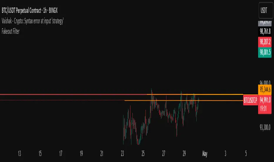
Fakeout Filter📈 Fakeout Filter by ARV
🔍 Overview:
The Fakeout Filter is a smart breakout validation tool designed to help traders avoid false breakouts and focus only on high-probability breakout trades. This indicator combines price action, volume analysis, RSI divergence detection, and OBV trend confirmation to filter out noise and improve your entries.
⚙️ Key Features:
✅ Breakout Detection
Detects when the price closes above a user-defined resistance level.
✅ Volume Spike Confirmation
Confirms breakouts only if there’s a significant increase in volume (customizable via settings).
✅ RSI Bearish Divergence Filter
Warns you of bearish RSI divergence, which often signals fakeouts during breakouts.
✅ OBV Trend Confirmation
Ensures On-Balance Volume (OBV) is rising, aligning volume flow with price movement.
✅ EMA Filter (Trend Confirmation)
Adds a safety filter using Exponential Moving Average (EMA) to ensure price action aligns with the short-term trend.
📌 How to Use:
Set Resistance Level:
In the indicator settings, input a key resistance level (manual input based on your chart analysis).
Watch for Signals:
A green background and “Breakout” label appear when:
Price closes above the resistance.
Volume is significantly higher than average.
OBV is rising.
No bearish RSI divergence is detected.
Price is above the EMA (trend confirmation).
Entry Suggestion:
Consider entering long positions only when the breakout label appears.
For additional confirmation, wait for a retest of the resistance as support before entering.
🔧 Settings:
Resistance Level – Manually set the level you're watching.
Volume Multiplier – Adjusts sensitivity to volume spikes (default: 1.5x average).
RSI Period – RSI used for divergence detection (default: 14).
EMA Period – For trend direction confirmation (default: 21).
✅ Best Use Cases:
Scalpers and intraday traders avoiding fakeouts on 5m–1H timeframes.
Swing traders validating breakout setups.
BTC, ETH, and major altcoins in consolidation or breakout zones.
⚠️ Disclaimer:
This tool is for educational purposes only. Always combine it with your own market analysis and risk management.
Cerca negli script per "OBV"
J Weighted Average Price📘 How to Use the OBV VWAP Reentry Signal Effectively
This indicator plots a VWAP based on OBV (On-Balance Volume), along with dynamic bands to identify overbought and oversold conditions in volume flow.
🔺 Red Triangle Up: Appears when OBV crosses back below the upper band → Potential reversal from overbought → Watch for short opportunities.
🔻 Blue Triangle Down: Appears when OBV crosses back above the lower band → Potential reversal from oversold → Watch for long opportunities.
📌 Tip: Use these signals in confluence with price action or trend confirmation to filter false signals. For example:
Enter short after a reentry from upper band and a lower high in price.
Enter long after a reentry from lower band and a bullish candle structure.
This setup helps you catch mean reversion moves based on volume flow, not just price.
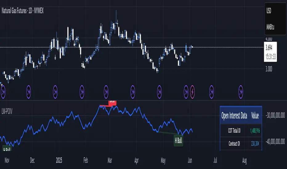
Larry Williams POIV A/D [tradeviZion]Larry Williams' POIV A/D - Release Notes v1.0
=================================================
Release Date: 01 April 2025
OVERVIEW
--------
The Larry Williams POIV A/D (Price, Open Interest, Volume Accumulation/Distribution) indicator implements Williams' original formula while adding advanced divergence detection capabilities. This powerful tool combines price movement, open interest, and volume data to identify potential trend reversals and continuations.
FEATURES
--------
- Implements Larry Williams' original POIV A/D formula
- Divergence detection system:
* Regular divergences for trend reversal signals
* Hidden divergences for trend continuation signals
- Fast Mode option for earlier pivot detection
- Customizable sensitivity for divergence filtering
- Dynamic color visualization based on indicator direction
- Adjustable smoothing to reduce noise
- Automatic fallback to OBV when Open Interest is unavailable
FORMULA
-------
POIV A/D = CumulativeSum(Open Interest * (Close - Close ) / (True High - True Low)) + OBV
Where:
- Open Interest: Current period's open interest
- Close - Close : Price change from previous period
- True High - True Low: True Range
- OBV: On Balance Volume
DIVERGENCE TYPES
---------------
1. Regular Divergences (Reversal Signals):
- Bullish: Price makes lower lows while indicator makes higher lows
- Bearish: Price makes higher highs while indicator makes lower highs
2. Hidden Divergences (Continuation Signals):
- Bullish: Price makes higher lows while indicator makes lower lows
- Bearish: Price makes lower highs while indicator makes higher highs
REQUIREMENTS
-----------
- Works best with futures and other instruments that provide Open Interest data
- Automatically adapts to work with any instrument by using OBV when OI is unavailable
USAGE GUIDE
-----------
1. Apply the indicator to any chart
2. Configure settings:
- Adjust sensitivity for divergence detection
- Enable/disable Fast Mode for earlier signals
- Customize visual settings as needed
3. Look for divergence signals:
- Regular divergences for potential trend reversals
- Hidden divergences for trend continuation opportunities
4. Use the alerts system for automated divergence detection
KNOWN LIMITATIONS
----------------
- Requires Open Interest data for full functionality
- Fast Mode may generate more signals but with lower reliability
ACKNOWLEDGEMENTS
---------------
This indicator is based on Larry Williams' work on Open Interest analysis. The implementation includes additional features for divergence detection while maintaining the integrity of the original formula.
Advanced Physics Financial Indicator Each component represents a scientific theory and is applied to the price data in a way that reflects key principles from that theory.
Detailed Explanation
1. Fractal Geometry - High/Low Signal
Concept: Fractal geometry studies self-similar patterns that repeat at different scales. In markets, fractals can be used to detect recurring patterns or turning points.
Implementation: The script detects pivot highs and lows using ta.pivothigh and ta.pivotlow, representing local turning points in price. The fractalSignal is set to 1 for a pivot high, -1 for a pivot low, and 0 if there is no signal. This logic reflects the cyclical, self-similar nature of price movements.
Practical Use: This signal is useful for identifying local tops and bottoms, allowing traders to spot potential reversals or consolidation points where fractal patterns emerge.
2. Quantum Mechanics - Probabilistic Monte Carlo Simulation
Concept: Quantum mechanics introduces uncertainty and probability into systems, much like how future price movements are inherently uncertain. Monte Carlo simulations are used to model a range of possible outcomes based on random inputs.
Implementation: In this script, we simulate 100 random outcomes by generating a random number between -1 and 1 for each iteration. These random values are stored in an array, and the average of these values is calculated to represent the Quantum Signal.
Practical Use: This probabilistic signal provides a sense of randomness and uncertainty in the market, reflecting the possibility of price movement in either direction. It simulates the market’s chaotic nature by considering multiple possible outcomes and their average.
3. Thermodynamics - Efficiency Ratio Signal
Concept: Thermodynamics deals with energy efficiency and entropy in systems. The efficiency ratio in financial terms can be used to measure how efficiently the price is moving relative to volatility.
Implementation: The Efficiency Ratio is calculated as the absolute price change over n periods divided by the sum of absolute changes for each period within n. This ratio shows how much of the price movement is directional versus random, mimicking the concept of efficiency in thermodynamic systems.
Practical Use: A high efficiency ratio suggests that the market is trending smoothly (high efficiency), while a low ratio indicates choppy, non-directional movement (low efficiency, or high entropy).
4. Chaos Theory - ATR Signal
Concept: Chaos theory studies how complex systems are highly sensitive to initial conditions, leading to unpredictable behavior. In markets, chaotic price movements can often be captured through volatility indicators.
Implementation: The script uses a very long ATR period (1000) to reflect slow-moving chaos over time. The Chaos Signal is computed by measuring the deviation of the current price from its long-term average (SMA), normalized by ATR. This captures price deviations over time, hinting at chaotic market behavior.
Practical Use: The signal measures how far the price deviates from its long-term average, which can signal the degree of chaos or extreme behavior in the market. High deviations indicate chaotic or volatile conditions, while low deviations suggest stability.
5. Network Theory - Correlation with BTC
Concept: Network theory studies how different components within a system are interconnected. In markets, assets are often correlated, meaning that price movements in one asset can influence or be influenced by another.
Implementation: This indicator calculates the correlation between the asset’s price and the price of Bitcoin (BTC) over 30 periods. The Network Signal shows how connected the asset is to BTC, reflecting broader market dynamics.
Practical Use: In a highly correlated market, BTC can act as a leading indicator for other assets. A strong correlation with BTC might suggest that the asset is likely to move in line with Bitcoin, while a weak or negative correlation might indicate that the asset is moving independently.
6. String Theory - RSI & MACD Interaction
Concept: String theory attempts to unify the fundamental forces of nature into a single framework. In trading, we can view the RSI and MACD as interacting forces that provide insights into momentum and trend.
Implementation: The script calculates the RSI and MACD and combines them into a single signal. The formula for String Signal is (RSI - 50) / 100 + (MACD Line - Signal Line) / 100, normalizing both indicators to a scale where their contributions are additive. The RSI represents momentum, and MACD shows trend direction and strength.
Practical Use: This signal helps in detecting moments where momentum (RSI) and trend strength (MACD) align, giving a clearer picture of the asset's direction and overbought/oversold conditions. It unifies these two indicators to create a more holistic view of market behavior.
7. Fluid Dynamics - On-Balance Volume (OBV) Signal
Concept: Fluid dynamics studies how fluids move and flow. In markets, volume can be seen as a "flow" that drives price movement, much like how fluid dynamics describe the flow of liquids.
Implementation: The script uses the OBV (On-Balance Volume) indicator to track the cumulative flow of volume based on price changes. The signal is further normalized by its moving average to smooth out fluctuations and make it more reflective of price pressure over time.
Practical Use: The Fluid Signal shows how the flow of volume is driving price action. If the OBV rises significantly, it suggests that there is strong buying pressure, while a falling OBV indicates selling pressure. It’s analogous to how pressure builds in a fluid system.
8. Final Signal - Combining All Physics-Based Indicators
Implementation: Each of the seven physics-inspired signals is combined into a single Final Signal by averaging their values. This approach blends different market insights from various scientific domains, creating a comprehensive view of the market’s condition.
Practical Use: The final signal gives you a holistic, multi-dimensional view of the market by merging different perspectives (fractal behavior, quantum probability, efficiency, chaos, correlation, momentum/trend, and volume flow). This approach helps traders understand the market's dynamics from multiple angles, offering deeper insights than any single indicator.
9. Color Coding Based on Signal Extremes
Concept: The color of the final signal plot dynamically reflects whether the market is in an extreme state.
Implementation: The signal color is determined using percentiles. If the Final Signal is in the top 55th percentile of its range, the signal is green (bullish). If it is between the 45th and 55th percentiles, it is orange (neutral). If it falls below the 45th percentile, it is red (bearish).
Practical Use: This visual representation helps traders quickly identify the strength of the signal. Bullish conditions (green), neutral conditions (orange), and bearish conditions (red) are clearly distinguished, simplifying decision-making.

MyLibrary_functions_D_S_3D_D_T_PART_1Library "MyLibrary_functions_D_S_3D_D_T_PART_1"
TODO: add library description here
color_(upcolor_txt, upcolor, dncolor_txt, dncolor, theme)
Parameters:
upcolor_txt (color)
upcolor (color)
dncolor_txt (color)
dncolor (color)
theme (string)
Source_Zigzag_F(Source)
Parameters:
Source (string)
p_lw_hg(Source_low, Source_high, Depth)
Parameters:
Source_low (float)
Source_high (float)
Depth (int)
lowing_highing(Source_low, Source_high, p_lw, p_hg, Deviation)
Parameters:
Source_low (float)
Source_high (float)
p_lw (int)
p_hg (int)
Deviation (int)
ll_lh(lowing, highing)
Parameters:
lowing (bool)
highing (bool)
down_ll_down_lh(ll, lh, Backstep)
Parameters:
ll (int)
lh (int)
Backstep (int)
down(down_ll, down_lh, lw, hg)
Parameters:
down_ll (bool)
down_lh (bool)
lw (int)
hg (int)
f_x_P_S123_lw(lw_, hg_, p_lw_, down, Source_low)
Parameters:
lw_ (int)
hg_ (int)
p_lw_ (int)
down (int)
Source_low (float)
f_x_P_S123_hg(lw_, hg_, p_hg_, down, Source_high)
Parameters:
lw_ (int)
hg_ (int)
p_hg_ (int)
down (int)
Source_high (float)
Update_lw_hg_last_l_last_h(lw, hg, last_l, last_h, p_lw, p_hg, down, Source_low, Source_high)
Parameters:
lw (int)
hg (int)
last_l (int)
last_h (int)
p_lw (int)
p_hg (int)
down (int)
Source_low (float)
Source_high (float)
x1_P_y1_P_x2_P_y2_P_x3_P_y3_P_x4_P_y4_P(lw, hg, last_l, last_h, Source)
Parameters:
lw (int)
hg (int)
last_l (int)
last_h (int)
Source (string)
x1_P_os(lw, hg, x2_D, Diverjence_MACD_Line_, Diverjence_MACD_Histagram_, Diverjence_RSI_, Diverjence_Stochastic_, Diverjence_volume_, Diverjence_CCI_, Diverjence_MFI_, Diverjence_Momentum_, Diverjence_OBV_, Diverjence_ADX_, MACD, hist_MACD, RSI, volume_ok, Stochastic_K, CCI, MFI, momentum, OBV, adx)
Parameters:
lw (int)
hg (int)
x2_D (int)
Diverjence_MACD_Line_ (bool)
Diverjence_MACD_Histagram_ (bool)
Diverjence_RSI_ (bool)
Diverjence_Stochastic_ (bool)
Diverjence_volume_ (bool)
Diverjence_CCI_ (bool)
Diverjence_MFI_ (bool)
Diverjence_Momentum_ (bool)
Diverjence_OBV_ (bool)
Diverjence_ADX_ (bool)
MACD (float)
hist_MACD (float)
RSI (float)
volume_ok (float)
Stochastic_K (float)
CCI (float)
MFI (float)
momentum (float)
OBV (float)
adx (float)
x3_P_os(lw, hg, x2_D, x4_D, Diverjence_MACD_Line_, Diverjence_MACD_Histagram_, Diverjence_RSI_, Diverjence_Stochastic_, Diverjence_volume_, Diverjence_CCI_, Diverjence_MFI_, Diverjence_Momentum_, Diverjence_OBV_, Diverjence_ADX_, MACD, hist_MACD, RSI, volume_ok, Stochastic_K, CCI, MFI, momentum, OBV, adx)
Parameters:
lw (int)
hg (int)
x2_D (int)
x4_D (int)
Diverjence_MACD_Line_ (bool)
Diverjence_MACD_Histagram_ (bool)
Diverjence_RSI_ (bool)
Diverjence_Stochastic_ (bool)
Diverjence_volume_ (bool)
Diverjence_CCI_ (bool)
Diverjence_MFI_ (bool)
Diverjence_Momentum_ (bool)
Diverjence_OBV_ (bool)
Diverjence_ADX_ (bool)
MACD (float)
hist_MACD (float)
RSI (float)
volume_ok (float)
Stochastic_K (float)
CCI (float)
MFI (float)
momentum (float)
OBV (float)
adx (float)
Err_test(lw, hg, x1, y1, x2, y2, y_d, start, finish, Err_Rate)
Parameters:
lw (int)
hg (int)
x1 (int)
y1 (float)
x2 (int)
y2 (float)
y_d (float)
start (int)
finish (int)
Err_Rate (float)
divergence_calculation(Feasibility_RD, Feasibility_HD, Feasibility_ED, lw, hg, Source_low, Source_high, x1_P_pr, x3_P_pr, x1_P_os, x3_P_os, x2_P_pr, x4_P_pr, oscillator, Fix_Err_Mid_Point_Pr, Fix_Err_Mid_Point_Os, Err_Rate_permissible_Mid_Line_Pr, Err_Rate_permissible_Mid_Line_Os, Number_of_price_periods_R_H, Permissible_deviation_factor_in_Pr_R_H, Number_of_oscillator_periods_R_H, Permissible_deviation_factor_in_OS_R_H, Number_of_price_periods_E, Permissible_deviation_factor_in_Pr_E, Number_of_oscillator_periods_E, Permissible_deviation_factor_in_OS_E)
Parameters:
Feasibility_RD (bool)
Feasibility_HD (bool)
Feasibility_ED (bool)
lw (int)
hg (int)
Source_low (float)
Source_high (float)
x1_P_pr (int)
x3_P_pr (int)
x1_P_os (int)
x3_P_os (int)
x2_P_pr (int)
x4_P_pr (int)
oscillator (float)
Fix_Err_Mid_Point_Pr (bool)
Fix_Err_Mid_Point_Os (bool)
Err_Rate_permissible_Mid_Line_Pr (float)
Err_Rate_permissible_Mid_Line_Os (float)
Number_of_price_periods_R_H (int)
Permissible_deviation_factor_in_Pr_R_H (float)
Number_of_oscillator_periods_R_H (int)
Permissible_deviation_factor_in_OS_R_H (float)
Number_of_price_periods_E (int)
Permissible_deviation_factor_in_Pr_E (float)
Number_of_oscillator_periods_E (int)
Permissible_deviation_factor_in_OS_E (float)
label_txt(label_ID, zigzag_Indicator_1_, zigzag_Indicator_2_, zigzag_Indicator_3_)
Parameters:
label_ID (string)
zigzag_Indicator_1_ (bool)
zigzag_Indicator_2_ (bool)
zigzag_Indicator_3_ (bool)
delet_scan_item_1(string_, NO_1, GAP)
Parameters:
string_ (string)
NO_1 (int)
GAP (int)
delet_scan_item_2(string_, NO_1, GAP)
Parameters:
string_ (string)
NO_1 (int)
GAP (int)
calculation_Final_total(MS_MN, Scan_zigzag_NO, zigzag_Indicator, zigzag_Indicator_1, zigzag_Indicator_2, zigzag_Indicator_3, LW_hg_P2, LW_hg_P1, lw_1, lw_2, lw_3, hg_1, hg_2, hg_3, lw_hg_D_POINT_ad_Array, lw_hg_D_POINT_id_Array, Array_Regular_MS, Array_Hidden_MS, Array_Exaggerated_MS, Array_Regular_MN, Array_Hidden_MN, Array_Exaggerated_MN)
Parameters:
MS_MN (string)
Scan_zigzag_NO (string)
zigzag_Indicator (bool)
zigzag_Indicator_1 (bool)
zigzag_Indicator_2 (bool)
zigzag_Indicator_3 (bool)
LW_hg_P2 (int)
LW_hg_P1 (int)
lw_1 (int)
lw_2 (int)
lw_3 (int)
hg_1 (int)
hg_2 (int)
hg_3 (int)
lw_hg_D_POINT_ad_Array (array)
lw_hg_D_POINT_id_Array (array)
Array_Regular_MS (array)
Array_Hidden_MS (array)
Array_Exaggerated_MS (array)
Array_Regular_MN (array)
Array_Hidden_MN (array)
Array_Exaggerated_MN (array)
Search_piote_1(array_id_7, scan_no)
Parameters:
array_id_7 (array)
scan_no (int)

Volume and Price Z-Score [Multi-Asset] - By LeviathanThis script offers in-depth Z-Score analytics on price and volume for 200 symbols. Utilizing visualizations such as scatter plots, histograms, and heatmaps, it enables traders to uncover potential trade opportunities, discern market dynamics, pinpoint outliers, delve into the relationship between price and volume, and much more.
A Z-Score is a statistical measurement indicating the number of standard deviations a data point deviates from the dataset's mean. Essentially, it provides insight into a value's relative position within a group of values (mean).
- A Z-Score of zero means the data point is exactly at the mean.
- A positive Z-Score indicates the data point is above the mean.
- A negative Z-Score indicates the data point is below the mean.
For instance, a Z-Score of 1 indicates that the data point is 1 standard deviation above the mean, while a Z-Score of -1 indicates that the data point is 1 standard deviation below the mean. In simple terms, the more extreme the Z-Score of a data point, the more “unusual” it is within a larger context.
If data is normally distributed, the following properties can be observed:
- About 68% of the data will lie within ±1 standard deviation (z-score between -1 and 1).
- About 95% will lie within ±2 standard deviations (z-score between -2 and 2).
- About 99.7% will lie within ±3 standard deviations (z-score between -3 and 3).
Datasets like price and volume (in this context) are most often not normally distributed. While the interpretation in terms of percentage of data lying within certain ranges of z-scores (like the ones mentioned above) won't hold, the z-score can still be a useful measure of how "unusual" a data point is relative to the mean.
The aim of this indicator is to offer a unique way of screening the market for trading opportunities by conveniently visualizing where current volume and price activity stands in relation to the average. It also offers features to observe the convergent/divergent relationships between asset’s price movement and volume, observe a single symbol’s activity compared to the wider market activity and much more.
Here is an overview of a few important settings.
Z-SCORE TYPE
◽️ Z-Score Type: Current Z-Score
Calculates the z-score by comparing current bar’s price and volume data to the mean (moving average with any custom length, default is 20 bars). This indicates how much the current bar’s price and volume data deviates from the average over the specified period. A positive z-score suggests that the current bar's price or volume is above the mean of the last 20 bars (or the custom length set by the user), while a negative z-score means it's below that mean.
Example: Consider an asset whose current price and volume both show deviations from their 20-bar averages. If the price's Z-Score is +1.5 and the volume's Z-Score is +2.0, it means the asset's price is 1.5 standard deviations above its average, and its trading volume is 2 standard deviations above its average. This might suggest a significant upward move with strong trading activity.
◽️ Z-Score Type: Average Z-Score
Calculates the custom-length average of symbol's z-score. Think of it as a smoothed version of the Current Z-Score. Instead of just looking at the z-score calculated on the latest bar, it considers the average behavior over the last few bars. By doing this, it helps reduce sudden jumps and gives a clearer, steadier view of the market.
Example: Instead of a single bar, imagine the average price and volume of an asset over the last 5 bars. If the price's 5-bar average Z-Score is +1.0 and the volume's is +1.5, it tells us that, over these recent bars, both the price and volume have been consistently above their longer-term averages, indicating sustained increase.
◽️ Z-Score Type: Relative Z-Score
Calculates a relative z-score by comparing symbol’s current bar z-score to the mean (average z-score of all symbols in the group). This is essentially a z-score of a z-score, and it helps in understanding how a particular symbol's activity stands out not just in its own historical context, but also in relation to the broader set of symbols being analyzed. In other words, while the primary z-score tells you how unusual a bar's activity is for that specific symbol, the relative z-score informs you how that "unusualness" ranks when compared to the entire group's deviations. This can be particularly useful in identifying symbols that are outliers even among outliers, indicating exceptionally unique behaviors or opportunities.
Example: If one asset's price Z-Score is +2.5 and volume Z-Score is +3.0, but the group's average Z-Scores are +0.5 for price and +1.0 for volume, this asset’s Relative Z-Score would be high and therefore stand out. This means that asset's price and volume activities are notably high, not just by its own standards, but also when compared to other symbols in the group.
DISPLAY TYPE
◽️ Display Type: Scatter Plot
The Scatter Plot is a visual tool designed to represent values for two variables, in this case the Z-Scores of price and volume for multiple symbols. Each symbol has it's own dot with x and y coordinates:
X-Axis: Represents the Z-Score of price. A symbol further to the right indicates a higher positive deviation in its price from its average, while a symbol to the left indicates a negative deviation.
Y-Axis: Represents the Z-Score of volume. A symbol positioned higher up on the plot suggests a higher positive deviation in its trading volume from its average, while one lower down indicates a negative deviation.
Here are some guideline insights of plot positioning:
- Top-Right Quadrant (High Volume-High Price): Symbols in this quadrant indicate a scenario where both the trading volume and price are higher than their respective mean.
- Top-Left Quadrant (High Volume-Low Price): Symbols here reflect high trading volumes but prices lower than the mean.
- Bottom-Left Quadrant (Low Volume-Low Price): Assets in this quadrant have both low trading volume and price compared to their mean.
- Bottom-Right Quadrant (Low Volume-High Price): Symbols positioned here have prices that are higher than their mean, but the trading volume is low compared to the mean.
The plot also integrates a set of concentric squares which serve as visual guides:
- 1st Square (1SD): Encapsulates symbols that have Z-Scores within ±1 standard deviation for both price and volume. Symbols within this square are typically considered to be displaying normal behavior or within expected range.
- 2nd Square (2SD): Encapsulates those with Z-Scores within ±2 standard deviations. Symbols within this boundary, but outside the 1 SD square, indicate a moderate deviation from the norm.
- 3rd Square (3SD): Represents symbols with Z-Scores within ±3 standard deviations. Any symbol outside this square is deemed to be a significant outlier, exhibiting extreme behavior in terms of either its price, its volume, or both.
By assessing the position of symbols relative to these squares, traders can swiftly identify which assets are behaving typically and which are showing unusual activity. This visualization simplifies the process of spotting potential outliers or unique trading opportunities within the market. The farther a symbol is from the center, the more it deviates from its typical behavior.
◽️ Display Type: Columns
In this visualization, z-scores are represented using columns, where each symbol is presented horizontally. Each symbol has two distinct nodes:
- Left Node: Represents the z-score of volume.
- Right Node: Represents the z-score of price.
The height of these nodes can vary along the y-axis between -4 and 4, based on the z-score value:
- Large Positive Columns: Signify a high or positive z-score, indicating that the price or volume is significantly above its average.
- Large Negative Columns: Represent a low or negative z-score, suggesting that the price or volume is considerably below its average.
- Short Columns Near 0: Indicate that the price or volume is close to its mean, showcasing minimal deviation.
This columnar representation provides a clear, intuitive view of how each symbol's price and volume deviate from their respective averages.
◽️ Display Type: Circles
In this visualization style, z-scores are depicted using circles. Each symbol is horizontally aligned and represented by:
- Solid Circle: Represents the z-score of price.
- Transparent Circle: Represents the z-score of volume.
The vertical position of these circles on the y-axis ranges between -4 and 4, reflecting the z-score value:
- Circles Near the Top: Indicate a high or positive z-score, suggesting the price or volume is well above its average.
- Circles Near the Bottom: Represent a low or negative z-score, pointing to the price or volume being notably below its average.
- Circles Around the Midline (0): Highlight that the price or volume is close to its mean, with minimal deviation.
◽️ Display Type: Delta Columns
There's also an option to utilize Z-Score Delta Columns. For each symbol, a single column is presented, depicting the difference between the z-score of price and the z-score of volume.
The z-score delta essentially captures the disparity between how much the price and volume deviate from their respective mean:
- Positive Delta: Indicates that the z-score of price is greater than the z-score of volume. This suggests that the price has deviated more from its average than the volume has from its own average. Such a scenario could point to price movements being more significant or pronounced compared to the changes in volume.
- Negative Delta: Represents that the z-score of volume is higher than the z-score of price. This might mean that there are substantial volume changes, yet the price hasn't moved as dramatically. This can be indicative of potential build-up in trading interest without an equivalent impact on price.
- Delta Close to 0: Means that the z-scores for price and volume are almost equal, indicating their deviations from the average are in sync.
◽️ Display Type: Z-Volume/Z-Price Heatmap
This visualization offers a heatmap either for volume z-scores or price z-scores across all symbols. Here's how it's presented:
Each symbol is allocated its own horizontal row. Within this row, bar-by-bar data is displayed using a color gradient to represent the z-score values. The heatmap employs a user-defined gradient scale, where a chosen "cold" color represents low z-scores and a chosen "hot" color signifies high z-scores. As the z-score increases or decreases, the colors transition smoothly along this gradient, providing an intuitive visual indication of the z-score's magnitude.
- Cold Colors: Indicate values significantly below the mean (negative z-score)
- Mild Colors: Represent values close to the mean, suggesting minimal deviation.
- Hot Colors: Indicate values significantly above the mean (positive z-score)
This heatmap format provides a rapid, visually impactful means to discern how each symbol's price or volume is behaving relative to its average. The color-coded rows allow you to quickly spot outliers.
VOLUME TYPE
The "Volume Type" input allows you to choose the nature of volume data that will be factored into the volume z-score calculation. The interpretation of indicator’s data changes based on this input. You can opt between:
- Volume (Regular Volume): This is the classic measure of trading volume, which represents the volume traded in a given time period - bar.
- OBV (On-Balance Volume): OBV is a momentum indicator that accumulates volume on up bars and subtracts it on down bars, making it a cumulative indicator that sort of measures buying and selling pressure.
Interpretation Implications:
- For Volume Type: Regular Volume:
Positive Z-Score: Indicates that the trading volume is above its average, meaning there's unusually high trading activity .
Negative Z-Score: Suggests that the trading volume is below its average, signifying unusually low trading activity.
- For Volume Type: OBV:
Positive Z-Score: Signifies that “buying pressure” is above its average.
Negative Z-Score: Signifies that “selling pressure” is above its average.
When comparing Z-Score of OBV to Z-Score of price, we can observe several scenarios. If Z-Price and Z-Volume are convergent (have similar z-scores), we can say that the directional price movement is supported by volume. If Z-Price and Z-Volume are divergent (have very different z-scores or one of them being zero), it suggests a potential misalignment between price movement and volume support, which might hint at possible reversals or weakness.

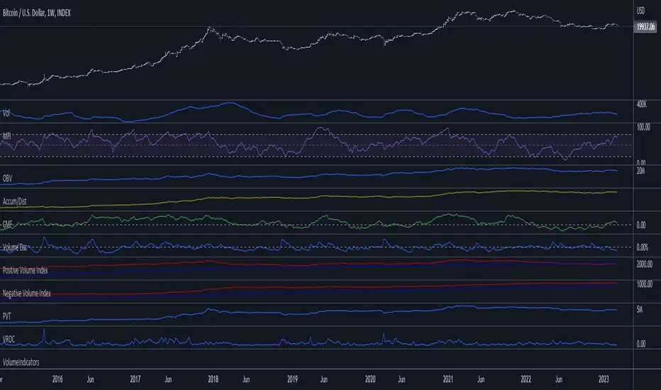
VolumeIndicatorsLibrary "VolumeIndicators"
This is a library of 'Volume Indicators'.
It aims to facilitate the grouping of this category of indicators, and also offer the customized supply of the source, not being restricted to just the closing price.
Indicators:
1. Volume Moving Average (VMA):
Moving average of volume. Identify trends in trading volume.
2. Money Flow Index (MFI): Measures volume pressure in a range of 0 to 100.
Calculates the ratio of volume when the price goes up and when the price goes down
3. On-Balance Volume (OBV):
Identify divergences between trading volume and an asset's price.
Sum of trading volume when the price rises and subtracts volume when the price falls.
4. Accumulation/Distribution (A/D):
Identifies buying and selling pressure by tracking the flow of money into and out of an asset based on volume patterns.
5. Chaikin Money Flow (CMF):
A variation of A/D that takes into account the daily price variation and weighs trading volume accordingly.
6. Volume Oscillator (VO):
Identify divergences between trading volume and an asset's price. Ratio of change of volume, from a fast period in relation to a long period.
7. Positive Volume Index (PVI):
Identify the upward strength of an asset. Volume when price rises divided by total volume.
8. Negative Volume Index (NVI):
Identify the downward strength of an asset. Volume when price falls divided by total volume.
9. Price-Volume Trend (PVT):
Identify the strength of an asset's price trend based on its trading volume. Cumulative change in price with volume factor
vma(length, maType, almaOffset, almaSigma, lsmaOffSet)
@description Volume Moving Average (VMA)
Parameters:
length : (int) Length for moving average
maType : (int) Type of moving average for smoothing
almaOffset : (float) Offset for Arnauld Legoux Moving Average
almaSigma : (float) Sigma for Arnauld Legoux Moving Average
lsmaOffSet : (float) Offset for Least Squares Moving Average
Returns: (float) Moving average of Volume
mfi(source, length)
@description MFI (Money Flow Index).
Uses both price and volume to measure buying and selling pressure in an asset.
Parameters:
source : (float) Source of series (close, high, low, etc.)
length
Returns: (float) Money Flow series
obv(source)
@description On Balance Volume (OBV)
Same as ta.obv(), but with customized type of source
Parameters:
source : (float) Series
Returns: (float) OBV
ad()
@description Accumulation/Distribution (A/D)
Returns: (float) Accumulation/Distribution (A/D) series
cmf(length)
@description CMF (Chaikin Money Flow).
Measures the flow of money into or out of an asset over time, using a combination of price and volume, and is used to identify the strength and direction of a trend.
Parameters:
length
Returns: (float) Chaikin Money Flow series
vo(shortLen, longLen, maType, almaOffset, almaSigma, lsmaOffSet)
@description Volume Oscillator (VO)
Parameters:
shortLen : (int) Fast period for volume
longLen : (int) Slow period for volume
maType : (int) Type of moving average for smoothing
almaOffset
almaSigma
lsmaOffSet
Returns: (float) Volume oscillator
pvi(source)
@description Positive Volume Index (PVI)
Same as ta.pvi(), but with customized type of source
Parameters:
source : (float) Series
Returns: (float) PVI
nvi(source)
@description Negative Volume Index (NVI)
Same as ta.nvi(), but with customized type of source
Parameters:
source : (float) Series
Returns: (float) PVI
pvt(source)
@description Price-Volume Trend (PVT)
Same as ta.pvt(), but with customized type of source
Parameters:
source : (float) Series
Returns: (float) PVI
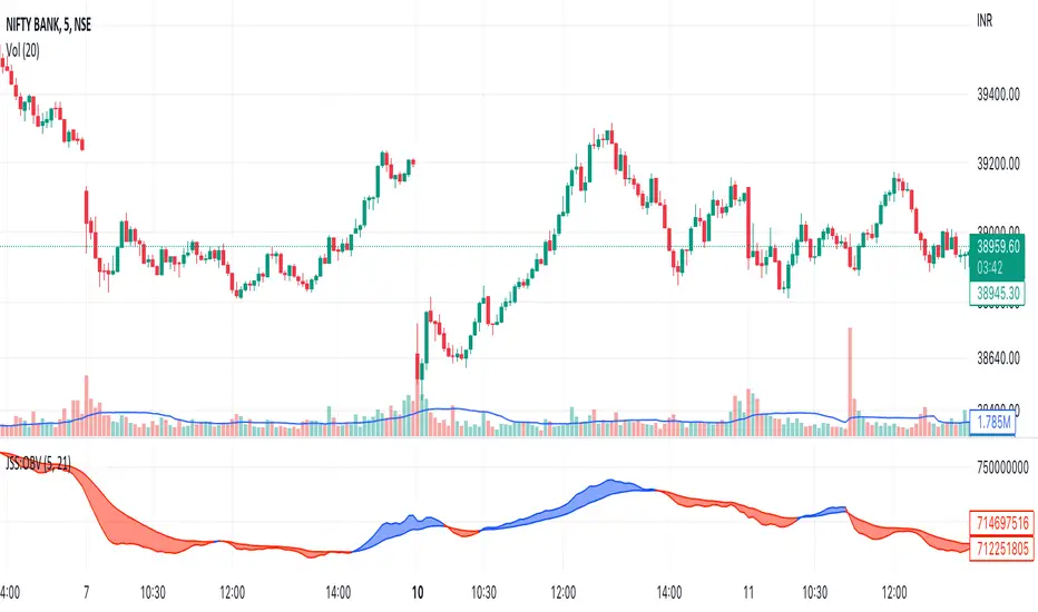
JSS: On Balance Volume//Date: 11-Oct-22
//Author: Jatinder Sodhi
OBV Indicator with colour coding.
Blue - Long
Red - Short
Best used for Intraday on 5 minute charts. Works well on other timeframes as well.
@Inspired by Asit Baran's RankDelta:OBV Indicator
//Not an exact replica as I have found one line correctly ema(obv,21)
//Whereas second line ema(obv,5) corresponds closely with Asit's indicator values but not exact.
//Advisable to use along with my RSI indicator based on Asit Baran's RankDelta:RSI indicator.
On-Balance Volume Oscillator with Divergence and PivotsThis is On-Balance Volume recalculated to be an Oscillator, a Divergence hunter was added, also Pivot Points and Alerts.
On-Balance Volume, or OBV is considered a "leading indicator" - in contrast to a "lagging indicator" just as Moving Averages it does not show a confirmation what already happened, but it shows what can happen in the future. For example: The chart is climbing while the OBV oscillator is slowly declining, gets weaker and weaker, maybe even prints bearish divergences? That means that a reversal might be occurring soon. Leading indicators are best paired with Stop and Resistance Lines, general Trendlines, Fib Retracements etc...Your chart is approaching a very important Resistance Trendline but the OBV shows a very positive signal? That means there is a high probability that the Resistance is going to be pushed though and becomes Support in the future.
What are those circles?
-These are Divergences. Red for Regular-Bearish. Orange for Hidden-Bearish. Green for Regular-Bullish. Aqua for Hidden-Bullish.
What are those triangles?
- These are Pivots. They show when the OBV oscillator might reverse, this is important to know because many times the price action follows this move.
Please keep in mind that this indicator is a tool and not a strategy, do not blindly trade signals, do your own research first! Use this indicator in conjunction with other indicators to get multiple confirmations.
On Balance Volume HLOC with AverageI am playing OBV now.
The original OBV is only calculate CLOSE.
I got an idea about XOBV with HLOC.
A bar has 5 periods:
- Open--Low--Open--Close--High--Close or
- Open--High--Open--Close--Low--Close
Assume that volume will evenly distributed on these 5 periods. Only Open--Close period has effective changed volume.
So XOBV = OBV * abs(close-open)/(2*(high-low)-abs(close-open)))
Better use XOBV and OBV both. Divergence and same price comparison are worth to watching.

On Balance Volume + Trend + DivergencesModification of original OBV indicator, with addition of Divergences identification & coloring OBV Line based on line (OBV either above or below EMA20 applied to OBV). Indicator works great in correlation with Volume, Stochastic and DMI and shows potential reversals earlier.

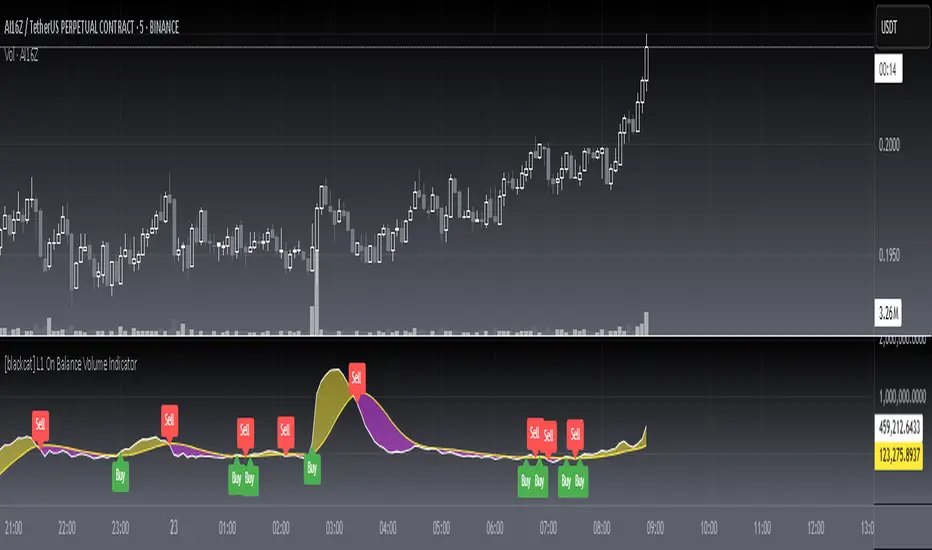
L1 On Balance Volume IndicatorLevel: 1
Background
On Balance Volume (OBV) is a simple indicator that uses volume and price to measure buying and selling pressure. The buying pressure is evident when the positive volume exceeds the negative volume and the OBV line rises.
Function
L1 On Balance Volume Indicator is a simple but improved OBV by using alma and more input parameters
Key Signal
OBV and its ALMA
Pros and Cons
Pros:
1. More freedom to tune with more input parameters
2. ALMA can make better tradeoff between response and smooth
Cons:
1. No details of volume generation can be disclosed
2. It may help to judge trend but not the short-term price movements.
Remarks
NA
Readme
In real life, I am a prolific inventor. I have successfully applied for more than 60 international and regional patents in the past 12 years. But in the past two years or so, I have tried to transfer my creativity to the development of trading strategies. Tradingview is the ideal platform for me. I am selecting and contributing some of the hundreds of scripts to publish in Tradingview community. Welcome everyone to interact with me to discuss these interesting pine scripts.
The scripts posted are categorized into 5 levels according to my efforts or manhours put into these works.
Level 1 : interesting script snippets or distinctive improvement from classic indicators or strategy. Level 1 scripts can usually appear in more complex indicators as a function module or element.
Level 2 : composite indicator/strategy. By selecting or combining several independent or dependent functions or sub indicators in proper way, the composite script exhibits a resonance phenomenon which can filter out noise or fake trading signal to enhance trading confidence level.
Level 3 : comprehensive indicator/strategy. They are simple trading systems based on my strategies. They are commonly containing several or all of entry signal, close signal, stop loss, take profit, re-entry, risk management, and position sizing techniques. Even some interesting fundamental and mass psychological aspects are incorporated.
Level 4 : script snippets or functions that do not disclose source code. Interesting element that can reveal market laws and work as raw material for indicators and strategies. If you find Level 1~2 scripts are helpful, Level 4 is a private version that took me far more efforts to develop.
Level 5 : indicator/strategy that do not disclose source code. private version of Level 3 script with my accumulated script processing skills or a large number of custom functions. I had a private function library built in past two years. Level 5 scripts use many of them to achieve private trading strategy.
PVT Osc - Price Volume Trend Oscillator [UTS]The oscillator version of the Price Volume Trend indicator (PVT) can be considered as a leading indicator of future price movements. The PVT Indicator is similar to the On Balance Volume indicator as it is also used to measure the strength of a trend.
The difference between the OBV and the PVT is that where the OBV adds all volumes when price achieves higher daily closes and subtracts them when price registers a lower daily close, the PVT adds or subtracts only a portion of the volume from the cumulative total in relation to a percentage change in price.
The general market consensus is that this difference enables the PVT to more accurately represent money flow volumes in and out of a stock or commodity.
The PVT has been designed so that it is capable of forecasting directional changes in price. For instance, if the price of a stock is rising and the PVT begins to fall, then this is indicative that a price reversal could occur very soon.
The general consensus is that the PVT is more accurate at detecting new trading opportunities than the OBV because of the differences in their construction. The OBV is designed so that it adds the same amount of volume whether the price closes upwards by just a small fraction or by multiples of its day opening value. On the other hand, the PVT adds volume proportional to the amount the price closed higher.
General Usage
Plain old PVT can be used to confirm trends, as well as spot possible trading signals due to divergences.
A benefit of the oscillator version is that it can produce LONG or SHORT signals on zero line cross.
Or controversy, disallow LONG trades in bearish territory and disallow SHORT trades in bullish territory.
Moving Averages
4 different Moving Averages are available:
EMA (Exponential Moving Average)
SMA (Simple Moving Average)
VWMA (Volume Weighted Moving Average)
WMA (Weighted Moving Average)

TA-Money Flow-Version5This is the MACD of a stochastic OBV movement indicator, Squeeze Momentum Indicator, and addition coloring for Market Direction Indicator . It is good (right) to work with both price and volume.
In this version we've moved the divergence highlighting to symbols at the ends of the histograms. Same coloring scheme as previous, yellow is divergence of either OBV or SQZ , red is both divergence. In the previous version we added in the "squeeze on - blue" highlighting to show follow through of divergence (or just squeeze/stall). We also added in another old script, but colors so well, Lazybears (Market Direction Indicator, linked below). Also incorporated a 3 color or 5 color scheme from the MDI script as a bool. It works great on any time frame, but you need to have volume data. Not sure where I originally got this (stoch-OBV, somewhere off Tradingview several years ago, thanks to the person who shared), Squeeze/MDI is Lazybear, links below.
Enjoy.
Version 5:
Moved divergence highlighting to symbols on histogram
Added coloring based on MDI
TA-Money-Flow-Version4
TA-Money-Flow-Version3
TA-Money-Flow-Version2
Squeeze-Momentum-Indicator-LazyBear
Market-Direction-Indicator-LazyBear
TA-Money Flow-Version3This is the MACD of a stochastic OBV movement indicator. It is good (right) to work with both price and volume. I've included highlighting based on price divergence. It works great on any time frame, but you need to have volume data. Not sure where I originally got this (stoch-OBV, somewhere off Tradingview several years ago, thanks to the person who shared), just publishing because of a request.
Enjoy.
Version 2 - TA-Money-Flow-v2-Stochastic-OBV

Markov Chain [3D] | FractalystWhat exactly is a Markov Chain?
This indicator uses a Markov Chain model to analyze, quantify, and visualize the transitions between market regimes (Bull, Bear, Neutral) on your chart. It dynamically detects these regimes in real-time, calculates transition probabilities, and displays them as animated 3D spheres and arrows, giving traders intuitive insight into current and future market conditions.
How does a Markov Chain work, and how should I read this spheres-and-arrows diagram?
Think of three weather modes: Sunny, Rainy, Cloudy.
Each sphere is one mode. The loop on a sphere means “stay the same next step” (e.g., Sunny again tomorrow).
The arrows leaving a sphere show where things usually go next if they change (e.g., Sunny moving to Cloudy).
Some paths matter more than others. A more prominent loop means the current mode tends to persist. A more prominent outgoing arrow means a change to that destination is the usual next step.
Direction isn’t symmetric: moving Sunny→Cloudy can behave differently than Cloudy→Sunny.
Now relabel the spheres to markets: Bull, Bear, Neutral.
Spheres: market regimes (uptrend, downtrend, range).
Self‑loop: tendency for the current regime to continue on the next bar.
Arrows: the most common next regime if a switch happens.
How to read: Start at the sphere that matches current bar state. If the loop stands out, expect continuation. If one outgoing path stands out, that switch is the typical next step. Opposite directions can differ (Bear→Neutral doesn’t have to match Neutral→Bear).
What states and transitions are shown?
The three market states visualized are:
Bullish (Bull): Upward or strong-market regime.
Bearish (Bear): Downward or weak-market regime.
Neutral: Sideways or range-bound regime.
Bidirectional animated arrows and probability labels show how likely the market is to move from one regime to another (e.g., Bull → Bear or Neutral → Bull).
How does the regime detection system work?
You can use either built-in price returns (based on adaptive Z-score normalization) or supply three custom indicators (such as volume, oscillators, etc.).
Values are statistically normalized (Z-scored) over a configurable lookback period.
The normalized outputs are classified into Bull, Bear, or Neutral zones.
If using three indicators, their regime signals are averaged and smoothed for robustness.
How are transition probabilities calculated?
On every confirmed bar, the algorithm tracks the sequence of detected market states, then builds a rolling window of transitions.
The code maintains a transition count matrix for all regime pairs (e.g., Bull → Bear).
Transition probabilities are extracted for each possible state change using Laplace smoothing for numerical stability, and frequently updated in real-time.
What is unique about the visualization?
3D animated spheres represent each regime and change visually when active.
Animated, bidirectional arrows reveal transition probabilities and allow you to see both dominant and less likely regime flows.
Particles (moving dots) animate along the arrows, enhancing the perception of regime flow direction and speed.
All elements dynamically update with each new price bar, providing a live market map in an intuitive, engaging format.
Can I use custom indicators for regime classification?
Yes! Enable the "Custom Indicators" switch and select any three chart series as inputs. These will be normalized and combined (each with equal weight), broadening the regime classification beyond just price-based movement.
What does the “Lookback Period” control?
Lookback Period (default: 100) sets how much historical data builds the probability matrix. Shorter periods adapt faster to regime changes but may be noisier. Longer periods are more stable but slower to adapt.
How is this different from a Hidden Markov Model (HMM)?
It sets the window for both regime detection and probability calculations. Lower values make the system more reactive, but potentially noisier. Higher values smooth estimates and make the system more robust.
How is this Markov Chain different from a Hidden Markov Model (HMM)?
Markov Chain (as here): All market regimes (Bull, Bear, Neutral) are directly observable on the chart. The transition matrix is built from actual detected regimes, keeping the model simple and interpretable.
Hidden Markov Model: The actual regimes are unobservable ("hidden") and must be inferred from market output or indicator "emissions" using statistical learning algorithms. HMMs are more complex, can capture more subtle structure, but are harder to visualize and require additional machine learning steps for training.
A standard Markov Chain models transitions between observable states using a simple transition matrix, while a Hidden Markov Model assumes the true states are hidden (latent) and must be inferred from observable “emissions” like price or volume data. In practical terms, a Markov Chain is transparent and easier to implement and interpret; an HMM is more expressive but requires statistical inference to estimate hidden states from data.
Markov Chain: states are observable; you directly count or estimate transition probabilities between visible states. This makes it simpler, faster, and easier to validate and tune.
HMM: states are hidden; you only observe emissions generated by those latent states. Learning involves machine learning/statistical algorithms (commonly Baum–Welch/EM for training and Viterbi for decoding) to infer both the transition dynamics and the most likely hidden state sequence from data.
How does the indicator avoid “repainting” or look-ahead bias?
All regime changes and matrix updates happen only on confirmed (closed) bars, so no future data is leaked, ensuring reliable real-time operation.
Are there practical tuning tips?
Tune the Lookback Period for your asset/timeframe: shorter for fast markets, longer for stability.
Use custom indicators if your asset has unique regime drivers.
Watch for rapid changes in transition probabilities as early warning of a possible regime shift.
Who is this indicator for?
Quants and quantitative researchers exploring probabilistic market modeling, especially those interested in regime-switching dynamics and Markov models.
Programmers and system developers who need a probabilistic regime filter for systematic and algorithmic backtesting:
The Markov Chain indicator is ideally suited for programmatic integration via its bias output (1 = Bull, 0 = Neutral, -1 = Bear).
Although the visualization is engaging, the core output is designed for automated, rules-based workflows—not for discretionary/manual trading decisions.
Developers can connect the indicator’s output directly to their Pine Script logic (using input.source()), allowing rapid and robust backtesting of regime-based strategies.
It acts as a plug-and-play regime filter: simply plug the bias output into your entry/exit logic, and you have a scientifically robust, probabilistically-derived signal for filtering, timing, position sizing, or risk regimes.
The MC's output is intentionally "trinary" (1/0/-1), focusing on clear regime states for unambiguous decision-making in code. If you require nuanced, multi-probability or soft-label state vectors, consider expanding the indicator or stacking it with a probability-weighted logic layer in your scripting.
Because it avoids subjectivity, this approach is optimal for systematic quants, algo developers building backtested, repeatable strategies based on probabilistic regime analysis.
What's the mathematical foundation behind this?
The mathematical foundation behind this Markov Chain indicator—and probabilistic regime detection in finance—draws from two principal models: the (standard) Markov Chain and the Hidden Markov Model (HMM).
How to use this indicator programmatically?
The Markov Chain indicator automatically exports a bias value (+1 for Bullish, -1 for Bearish, 0 for Neutral) as a plot visible in the Data Window. This allows you to integrate its regime signal into your own scripts and strategies for backtesting, automation, or live trading.
Step-by-Step Integration with Pine Script (input.source)
Add the Markov Chain indicator to your chart.
This must be done first, since your custom script will "pull" the bias signal from the indicator's plot.
In your strategy, create an input using input.source()
Example:
//@version=5
strategy("MC Bias Strategy Example")
mcBias = input.source(close, "MC Bias Source")
After saving, go to your script’s settings. For the “MC Bias Source” input, select the plot/output of the Markov Chain indicator (typically its bias plot).
Use the bias in your trading logic
Example (long only on Bull, flat otherwise):
if mcBias == 1
strategy.entry("Long", strategy.long)
else
strategy.close("Long")
For more advanced workflows, combine mcBias with additional filters or trailing stops.
How does this work behind-the-scenes?
TradingView’s input.source() lets you use any plot from another indicator as a real-time, “live” data feed in your own script (source).
The selected bias signal is available to your Pine code as a variable, enabling logical decisions based on regime (trend-following, mean-reversion, etc.).
This enables powerful strategy modularity : decouple regime detection from entry/exit logic, allowing fast experimentation without rewriting core signal code.
Integrating 45+ Indicators with Your Markov Chain — How & Why
The Enhanced Custom Indicators Export script exports a massive suite of over 45 technical indicators—ranging from classic momentum (RSI, MACD, Stochastic, etc.) to trend, volume, volatility, and oscillator tools—all pre-calculated, centered/scaled, and available as plots.
// Enhanced Custom Indicators Export - 45 Technical Indicators
// Comprehensive technical analysis suite for advanced market regime detection
//@version=6
indicator('Enhanced Custom Indicators Export | Fractalyst', shorttitle='Enhanced CI Export', overlay=false, scale=scale.right, max_labels_count=500, max_lines_count=500)
// |----- Input Parameters -----| //
momentum_group = "Momentum Indicators"
trend_group = "Trend Indicators"
volume_group = "Volume Indicators"
volatility_group = "Volatility Indicators"
oscillator_group = "Oscillator Indicators"
display_group = "Display Settings"
// Common lengths
length_14 = input.int(14, "Standard Length (14)", minval=1, maxval=100, group=momentum_group)
length_20 = input.int(20, "Medium Length (20)", minval=1, maxval=200, group=trend_group)
length_50 = input.int(50, "Long Length (50)", minval=1, maxval=200, group=trend_group)
// Display options
show_table = input.bool(true, "Show Values Table", group=display_group)
table_size = input.string("Small", "Table Size", options= , group=display_group)
// |----- MOMENTUM INDICATORS (15 indicators) -----| //
// 1. RSI (Relative Strength Index)
rsi_14 = ta.rsi(close, length_14)
rsi_centered = rsi_14 - 50
// 2. Stochastic Oscillator
stoch_k = ta.stoch(close, high, low, length_14)
stoch_d = ta.sma(stoch_k, 3)
stoch_centered = stoch_k - 50
// 3. Williams %R
williams_r = ta.stoch(close, high, low, length_14) - 100
// 4. MACD (Moving Average Convergence Divergence)
= ta.macd(close, 12, 26, 9)
// 5. Momentum (Rate of Change)
momentum = ta.mom(close, length_14)
momentum_pct = (momentum / close ) * 100
// 6. Rate of Change (ROC)
roc = ta.roc(close, length_14)
// 7. Commodity Channel Index (CCI)
cci = ta.cci(close, length_20)
// 8. Money Flow Index (MFI)
mfi = ta.mfi(close, length_14)
mfi_centered = mfi - 50
// 9. Awesome Oscillator (AO)
ao = ta.sma(hl2, 5) - ta.sma(hl2, 34)
// 10. Accelerator Oscillator (AC)
ac = ao - ta.sma(ao, 5)
// 11. Chande Momentum Oscillator (CMO)
cmo = ta.cmo(close, length_14)
// 12. Detrended Price Oscillator (DPO)
dpo = close - ta.sma(close, length_20)
// 13. Price Oscillator (PPO)
ppo = ta.sma(close, 12) - ta.sma(close, 26)
ppo_pct = (ppo / ta.sma(close, 26)) * 100
// 14. TRIX
trix_ema1 = ta.ema(close, length_14)
trix_ema2 = ta.ema(trix_ema1, length_14)
trix_ema3 = ta.ema(trix_ema2, length_14)
trix = ta.roc(trix_ema3, 1) * 10000
// 15. Klinger Oscillator
klinger = ta.ema(volume * (high + low + close) / 3, 34) - ta.ema(volume * (high + low + close) / 3, 55)
// 16. Fisher Transform
fisher_hl2 = 0.5 * (hl2 - ta.lowest(hl2, 10)) / (ta.highest(hl2, 10) - ta.lowest(hl2, 10)) - 0.25
fisher = 0.5 * math.log((1 + fisher_hl2) / (1 - fisher_hl2))
// 17. Stochastic RSI
stoch_rsi = ta.stoch(rsi_14, rsi_14, rsi_14, length_14)
stoch_rsi_centered = stoch_rsi - 50
// 18. Relative Vigor Index (RVI)
rvi_num = ta.swma(close - open)
rvi_den = ta.swma(high - low)
rvi = rvi_den != 0 ? rvi_num / rvi_den : 0
// 19. Balance of Power (BOP)
bop = (close - open) / (high - low)
// |----- TREND INDICATORS (10 indicators) -----| //
// 20. Simple Moving Average Momentum
sma_20 = ta.sma(close, length_20)
sma_momentum = ((close - sma_20) / sma_20) * 100
// 21. Exponential Moving Average Momentum
ema_20 = ta.ema(close, length_20)
ema_momentum = ((close - ema_20) / ema_20) * 100
// 22. Parabolic SAR
sar = ta.sar(0.02, 0.02, 0.2)
sar_trend = close > sar ? 1 : -1
// 23. Linear Regression Slope
lr_slope = ta.linreg(close, length_20, 0) - ta.linreg(close, length_20, 1)
// 24. Moving Average Convergence (MAC)
mac = ta.sma(close, 10) - ta.sma(close, 30)
// 25. Trend Intensity Index (TII)
tii_sum = 0.0
for i = 1 to length_20
tii_sum += close > close ? 1 : 0
tii = (tii_sum / length_20) * 100
// 26. Ichimoku Cloud Components
ichimoku_tenkan = (ta.highest(high, 9) + ta.lowest(low, 9)) / 2
ichimoku_kijun = (ta.highest(high, 26) + ta.lowest(low, 26)) / 2
ichimoku_signal = ichimoku_tenkan > ichimoku_kijun ? 1 : -1
// 27. MESA Adaptive Moving Average (MAMA)
mama_alpha = 2.0 / (length_20 + 1)
mama = ta.ema(close, length_20)
mama_momentum = ((close - mama) / mama) * 100
// 28. Zero Lag Exponential Moving Average (ZLEMA)
zlema_lag = math.round((length_20 - 1) / 2)
zlema_data = close + (close - close )
zlema = ta.ema(zlema_data, length_20)
zlema_momentum = ((close - zlema) / zlema) * 100
// |----- VOLUME INDICATORS (6 indicators) -----| //
// 29. On-Balance Volume (OBV)
obv = ta.obv
// 30. Volume Rate of Change (VROC)
vroc = ta.roc(volume, length_14)
// 31. Price Volume Trend (PVT)
pvt = ta.pvt
// 32. Negative Volume Index (NVI)
nvi = 0.0
nvi := volume < volume ? nvi + ((close - close ) / close ) * nvi : nvi
// 33. Positive Volume Index (PVI)
pvi = 0.0
pvi := volume > volume ? pvi + ((close - close ) / close ) * pvi : pvi
// 34. Volume Oscillator
vol_osc = ta.sma(volume, 5) - ta.sma(volume, 10)
// 35. Ease of Movement (EOM)
eom_distance = high - low
eom_box_height = volume / 1000000
eom = eom_box_height != 0 ? eom_distance / eom_box_height : 0
eom_sma = ta.sma(eom, length_14)
// 36. Force Index
force_index = volume * (close - close )
force_index_sma = ta.sma(force_index, length_14)
// |----- VOLATILITY INDICATORS (10 indicators) -----| //
// 37. Average True Range (ATR)
atr = ta.atr(length_14)
atr_pct = (atr / close) * 100
// 38. Bollinger Bands Position
bb_basis = ta.sma(close, length_20)
bb_dev = 2.0 * ta.stdev(close, length_20)
bb_upper = bb_basis + bb_dev
bb_lower = bb_basis - bb_dev
bb_position = bb_dev != 0 ? (close - bb_basis) / bb_dev : 0
bb_width = bb_dev != 0 ? (bb_upper - bb_lower) / bb_basis * 100 : 0
// 39. Keltner Channels Position
kc_basis = ta.ema(close, length_20)
kc_range = ta.ema(ta.tr, length_20)
kc_upper = kc_basis + (2.0 * kc_range)
kc_lower = kc_basis - (2.0 * kc_range)
kc_position = kc_range != 0 ? (close - kc_basis) / kc_range : 0
// 40. Donchian Channels Position
dc_upper = ta.highest(high, length_20)
dc_lower = ta.lowest(low, length_20)
dc_basis = (dc_upper + dc_lower) / 2
dc_position = (dc_upper - dc_lower) != 0 ? (close - dc_basis) / (dc_upper - dc_lower) : 0
// 41. Standard Deviation
std_dev = ta.stdev(close, length_20)
std_dev_pct = (std_dev / close) * 100
// 42. Relative Volatility Index (RVI)
rvi_up = ta.stdev(close > close ? close : 0, length_14)
rvi_down = ta.stdev(close < close ? close : 0, length_14)
rvi_total = rvi_up + rvi_down
rvi_volatility = rvi_total != 0 ? (rvi_up / rvi_total) * 100 : 50
// 43. Historical Volatility
hv_returns = math.log(close / close )
hv = ta.stdev(hv_returns, length_20) * math.sqrt(252) * 100
// 44. Garman-Klass Volatility
gk_vol = math.log(high/low) * math.log(high/low) - (2*math.log(2)-1) * math.log(close/open) * math.log(close/open)
gk_volatility = math.sqrt(ta.sma(gk_vol, length_20)) * 100
// 45. Parkinson Volatility
park_vol = math.log(high/low) * math.log(high/low)
parkinson = math.sqrt(ta.sma(park_vol, length_20) / (4 * math.log(2))) * 100
// 46. Rogers-Satchell Volatility
rs_vol = math.log(high/close) * math.log(high/open) + math.log(low/close) * math.log(low/open)
rogers_satchell = math.sqrt(ta.sma(rs_vol, length_20)) * 100
// |----- OSCILLATOR INDICATORS (5 indicators) -----| //
// 47. Elder Ray Index
elder_bull = high - ta.ema(close, 13)
elder_bear = low - ta.ema(close, 13)
elder_power = elder_bull + elder_bear
// 48. Schaff Trend Cycle (STC)
stc_macd = ta.ema(close, 23) - ta.ema(close, 50)
stc_k = ta.stoch(stc_macd, stc_macd, stc_macd, 10)
stc_d = ta.ema(stc_k, 3)
stc = ta.stoch(stc_d, stc_d, stc_d, 10)
// 49. Coppock Curve
coppock_roc1 = ta.roc(close, 14)
coppock_roc2 = ta.roc(close, 11)
coppock = ta.wma(coppock_roc1 + coppock_roc2, 10)
// 50. Know Sure Thing (KST)
kst_roc1 = ta.roc(close, 10)
kst_roc2 = ta.roc(close, 15)
kst_roc3 = ta.roc(close, 20)
kst_roc4 = ta.roc(close, 30)
kst = ta.sma(kst_roc1, 10) + 2*ta.sma(kst_roc2, 10) + 3*ta.sma(kst_roc3, 10) + 4*ta.sma(kst_roc4, 15)
// 51. Percentage Price Oscillator (PPO)
ppo_line = ((ta.ema(close, 12) - ta.ema(close, 26)) / ta.ema(close, 26)) * 100
ppo_signal = ta.ema(ppo_line, 9)
ppo_histogram = ppo_line - ppo_signal
// |----- PLOT MAIN INDICATORS -----| //
// Plot key momentum indicators
plot(rsi_centered, title="01_RSI_Centered", color=color.purple, linewidth=1)
plot(stoch_centered, title="02_Stoch_Centered", color=color.blue, linewidth=1)
plot(williams_r, title="03_Williams_R", color=color.red, linewidth=1)
plot(macd_histogram, title="04_MACD_Histogram", color=color.orange, linewidth=1)
plot(cci, title="05_CCI", color=color.green, linewidth=1)
// Plot trend indicators
plot(sma_momentum, title="06_SMA_Momentum", color=color.navy, linewidth=1)
plot(ema_momentum, title="07_EMA_Momentum", color=color.maroon, linewidth=1)
plot(sar_trend, title="08_SAR_Trend", color=color.teal, linewidth=1)
plot(lr_slope, title="09_LR_Slope", color=color.lime, linewidth=1)
plot(mac, title="10_MAC", color=color.fuchsia, linewidth=1)
// Plot volatility indicators
plot(atr_pct, title="11_ATR_Pct", color=color.yellow, linewidth=1)
plot(bb_position, title="12_BB_Position", color=color.aqua, linewidth=1)
plot(kc_position, title="13_KC_Position", color=color.olive, linewidth=1)
plot(std_dev_pct, title="14_StdDev_Pct", color=color.silver, linewidth=1)
plot(bb_width, title="15_BB_Width", color=color.gray, linewidth=1)
// Plot volume indicators
plot(vroc, title="16_VROC", color=color.blue, linewidth=1)
plot(eom_sma, title="17_EOM", color=color.red, linewidth=1)
plot(vol_osc, title="18_Vol_Osc", color=color.green, linewidth=1)
plot(force_index_sma, title="19_Force_Index", color=color.orange, linewidth=1)
plot(obv, title="20_OBV", color=color.purple, linewidth=1)
// Plot additional oscillators
plot(ao, title="21_Awesome_Osc", color=color.navy, linewidth=1)
plot(cmo, title="22_CMO", color=color.maroon, linewidth=1)
plot(dpo, title="23_DPO", color=color.teal, linewidth=1)
plot(trix, title="24_TRIX", color=color.lime, linewidth=1)
plot(fisher, title="25_Fisher", color=color.fuchsia, linewidth=1)
// Plot more momentum indicators
plot(mfi_centered, title="26_MFI_Centered", color=color.yellow, linewidth=1)
plot(ac, title="27_AC", color=color.aqua, linewidth=1)
plot(ppo_pct, title="28_PPO_Pct", color=color.olive, linewidth=1)
plot(stoch_rsi_centered, title="29_StochRSI_Centered", color=color.silver, linewidth=1)
plot(klinger, title="30_Klinger", color=color.gray, linewidth=1)
// Plot trend continuation
plot(tii, title="31_TII", color=color.blue, linewidth=1)
plot(ichimoku_signal, title="32_Ichimoku_Signal", color=color.red, linewidth=1)
plot(mama_momentum, title="33_MAMA_Momentum", color=color.green, linewidth=1)
plot(zlema_momentum, title="34_ZLEMA_Momentum", color=color.orange, linewidth=1)
plot(bop, title="35_BOP", color=color.purple, linewidth=1)
// Plot volume continuation
plot(nvi, title="36_NVI", color=color.navy, linewidth=1)
plot(pvi, title="37_PVI", color=color.maroon, linewidth=1)
plot(momentum_pct, title="38_Momentum_Pct", color=color.teal, linewidth=1)
plot(roc, title="39_ROC", color=color.lime, linewidth=1)
plot(rvi, title="40_RVI", color=color.fuchsia, linewidth=1)
// Plot volatility continuation
plot(dc_position, title="41_DC_Position", color=color.yellow, linewidth=1)
plot(rvi_volatility, title="42_RVI_Volatility", color=color.aqua, linewidth=1)
plot(hv, title="43_Historical_Vol", color=color.olive, linewidth=1)
plot(gk_volatility, title="44_GK_Volatility", color=color.silver, linewidth=1)
plot(parkinson, title="45_Parkinson_Vol", color=color.gray, linewidth=1)
// Plot final oscillators
plot(rogers_satchell, title="46_RS_Volatility", color=color.blue, linewidth=1)
plot(elder_power, title="47_Elder_Power", color=color.red, linewidth=1)
plot(stc, title="48_STC", color=color.green, linewidth=1)
plot(coppock, title="49_Coppock", color=color.orange, linewidth=1)
plot(kst, title="50_KST", color=color.purple, linewidth=1)
// Plot final indicators
plot(ppo_histogram, title="51_PPO_Histogram", color=color.navy, linewidth=1)
plot(pvt, title="52_PVT", color=color.maroon, linewidth=1)
// |----- Reference Lines -----| //
hline(0, "Zero Line", color=color.gray, linestyle=hline.style_dashed, linewidth=1)
hline(50, "Midline", color=color.gray, linestyle=hline.style_dotted, linewidth=1)
hline(-50, "Lower Midline", color=color.gray, linestyle=hline.style_dotted, linewidth=1)
hline(25, "Upper Threshold", color=color.gray, linestyle=hline.style_dotted, linewidth=1)
hline(-25, "Lower Threshold", color=color.gray, linestyle=hline.style_dotted, linewidth=1)
// |----- Enhanced Information Table -----| //
if show_table and barstate.islast
table_position = position.top_right
table_text_size = table_size == "Tiny" ? size.tiny : table_size == "Small" ? size.small : size.normal
var table info_table = table.new(table_position, 3, 18, bgcolor=color.new(color.white, 85), border_width=1, border_color=color.gray)
// Headers
table.cell(info_table, 0, 0, 'Category', text_color=color.black, text_size=table_text_size, bgcolor=color.new(color.blue, 70))
table.cell(info_table, 1, 0, 'Indicator', text_color=color.black, text_size=table_text_size, bgcolor=color.new(color.blue, 70))
table.cell(info_table, 2, 0, 'Value', text_color=color.black, text_size=table_text_size, bgcolor=color.new(color.blue, 70))
// Key Momentum Indicators
table.cell(info_table, 0, 1, 'MOMENTUM', text_color=color.purple, text_size=table_text_size, bgcolor=color.new(color.purple, 90))
table.cell(info_table, 1, 1, 'RSI Centered', text_color=color.purple, text_size=table_text_size)
table.cell(info_table, 2, 1, str.tostring(rsi_centered, '0.00'), text_color=color.purple, text_size=table_text_size)
table.cell(info_table, 0, 2, '', text_color=color.blue, text_size=table_text_size)
table.cell(info_table, 1, 2, 'Stoch Centered', text_color=color.blue, text_size=table_text_size)
table.cell(info_table, 2, 2, str.tostring(stoch_centered, '0.00'), text_color=color.blue, text_size=table_text_size)
table.cell(info_table, 0, 3, '', text_color=color.red, text_size=table_text_size)
table.cell(info_table, 1, 3, 'Williams %R', text_color=color.red, text_size=table_text_size)
table.cell(info_table, 2, 3, str.tostring(williams_r, '0.00'), text_color=color.red, text_size=table_text_size)
table.cell(info_table, 0, 4, '', text_color=color.orange, text_size=table_text_size)
table.cell(info_table, 1, 4, 'MACD Histogram', text_color=color.orange, text_size=table_text_size)
table.cell(info_table, 2, 4, str.tostring(macd_histogram, '0.000'), text_color=color.orange, text_size=table_text_size)
table.cell(info_table, 0, 5, '', text_color=color.green, text_size=table_text_size)
table.cell(info_table, 1, 5, 'CCI', text_color=color.green, text_size=table_text_size)
table.cell(info_table, 2, 5, str.tostring(cci, '0.00'), text_color=color.green, text_size=table_text_size)
// Key Trend Indicators
table.cell(info_table, 0, 6, 'TREND', text_color=color.navy, text_size=table_text_size, bgcolor=color.new(color.navy, 90))
table.cell(info_table, 1, 6, 'SMA Momentum %', text_color=color.navy, text_size=table_text_size)
table.cell(info_table, 2, 6, str.tostring(sma_momentum, '0.00'), text_color=color.navy, text_size=table_text_size)
table.cell(info_table, 0, 7, '', text_color=color.maroon, text_size=table_text_size)
table.cell(info_table, 1, 7, 'EMA Momentum %', text_color=color.maroon, text_size=table_text_size)
table.cell(info_table, 2, 7, str.tostring(ema_momentum, '0.00'), text_color=color.maroon, text_size=table_text_size)
table.cell(info_table, 0, 8, '', text_color=color.teal, text_size=table_text_size)
table.cell(info_table, 1, 8, 'SAR Trend', text_color=color.teal, text_size=table_text_size)
table.cell(info_table, 2, 8, str.tostring(sar_trend, '0'), text_color=color.teal, text_size=table_text_size)
table.cell(info_table, 0, 9, '', text_color=color.lime, text_size=table_text_size)
table.cell(info_table, 1, 9, 'Linear Regression', text_color=color.lime, text_size=table_text_size)
table.cell(info_table, 2, 9, str.tostring(lr_slope, '0.000'), text_color=color.lime, text_size=table_text_size)
// Key Volatility Indicators
table.cell(info_table, 0, 10, 'VOLATILITY', text_color=color.yellow, text_size=table_text_size, bgcolor=color.new(color.yellow, 90))
table.cell(info_table, 1, 10, 'ATR %', text_color=color.yellow, text_size=table_text_size)
table.cell(info_table, 2, 10, str.tostring(atr_pct, '0.00'), text_color=color.yellow, text_size=table_text_size)
table.cell(info_table, 0, 11, '', text_color=color.aqua, text_size=table_text_size)
table.cell(info_table, 1, 11, 'BB Position', text_color=color.aqua, text_size=table_text_size)
table.cell(info_table, 2, 11, str.tostring(bb_position, '0.00'), text_color=color.aqua, text_size=table_text_size)
table.cell(info_table, 0, 12, '', text_color=color.olive, text_size=table_text_size)
table.cell(info_table, 1, 12, 'KC Position', text_color=color.olive, text_size=table_text_size)
table.cell(info_table, 2, 12, str.tostring(kc_position, '0.00'), text_color=color.olive, text_size=table_text_size)
// Key Volume Indicators
table.cell(info_table, 0, 13, 'VOLUME', text_color=color.blue, text_size=table_text_size, bgcolor=color.new(color.blue, 90))
table.cell(info_table, 1, 13, 'Volume ROC', text_color=color.blue, text_size=table_text_size)
table.cell(info_table, 2, 13, str.tostring(vroc, '0.00'), text_color=color.blue, text_size=table_text_size)
table.cell(info_table, 0, 14, '', text_color=color.red, text_size=table_text_size)
table.cell(info_table, 1, 14, 'EOM', text_color=color.red, text_size=table_text_size)
table.cell(info_table, 2, 14, str.tostring(eom_sma, '0.000'), text_color=color.red, text_size=table_text_size)
// Key Oscillators
table.cell(info_table, 0, 15, 'OSCILLATORS', text_color=color.purple, text_size=table_text_size, bgcolor=color.new(color.purple, 90))
table.cell(info_table, 1, 15, 'Awesome Osc', text_color=color.blue, text_size=table_text_size)
table.cell(info_table, 2, 15, str.tostring(ao, '0.000'), text_color=color.blue, text_size=table_text_size)
table.cell(info_table, 0, 16, '', text_color=color.red, text_size=table_text_size)
table.cell(info_table, 1, 16, 'Fisher Transform', text_color=color.red, text_size=table_text_size)
table.cell(info_table, 2, 16, str.tostring(fisher, '0.000'), text_color=color.red, text_size=table_text_size)
// Summary Statistics
table.cell(info_table, 0, 17, 'SUMMARY', text_color=color.black, text_size=table_text_size, bgcolor=color.new(color.gray, 70))
table.cell(info_table, 1, 17, 'Total Indicators: 52', text_color=color.black, text_size=table_text_size)
regime_color = rsi_centered > 10 ? color.green : rsi_centered < -10 ? color.red : color.gray
regime_text = rsi_centered > 10 ? "BULLISH" : rsi_centered < -10 ? "BEARISH" : "NEUTRAL"
table.cell(info_table, 2, 17, regime_text, text_color=regime_color, text_size=table_text_size)
This makes it the perfect “indicator backbone” for quantitative and systematic traders who want to prototype, combine, and test new regime detection models—especially in combination with the Markov Chain indicator.
How to use this script with the Markov Chain for research and backtesting:
Add the Enhanced Indicator Export to your chart.
Every calculated indicator is available as an individual data stream.
Connect the indicator(s) you want as custom input(s) to the Markov Chain’s “Custom Indicators” option.
In the Markov Chain indicator’s settings, turn ON the custom indicator mode.
For each of the three custom indicator inputs, select the exported plot from the Enhanced Export script—the menu lists all 45+ signals by name.
This creates a powerful, modular regime-detection engine where you can mix-and-match momentum, trend, volume, or custom combinations for advanced filtering.
Backtest regime logic directly.
Once you’ve connected your chosen indicators, the Markov Chain script performs regime detection (Bull/Neutral/Bear) based on your selected features—not just price returns.
The regime detection is robust, automatically normalized (using Z-score), and outputs bias (1, -1, 0) for plug-and-play integration.
Export the regime bias for programmatic use.
As described above, use input.source() in your Pine Script strategy or system and link the bias output.
You can now filter signals, control trade direction/size, or design pairs-trading that respect true, indicator-driven market regimes.
With this framework, you’re not limited to static or simplistic regime filters. You can rigorously define, test, and refine what “market regime” means for your strategies—using the technical features that matter most to you.
Optimize your signal generation by backtesting across a universe of meaningful indicator blends.
Enhance risk management with objective, real-time regime boundaries.
Accelerate your research: iterate quickly, swap indicator components, and see results with minimal code changes.
Automate multi-asset or pairs-trading by integrating regime context directly into strategy logic.
Add both scripts to your chart, connect your preferred features, and start investigating your best regime-based trades—entirely within the TradingView ecosystem.
References & Further Reading
Ang, A., & Bekaert, G. (2002). “Regime Switches in Interest Rates.” Journal of Business & Economic Statistics, 20(2), 163–182.
Hamilton, J. D. (1989). “A New Approach to the Economic Analysis of Nonstationary Time Series and the Business Cycle.” Econometrica, 57(2), 357–384.
Markov, A. A. (1906). "Extension of the Limit Theorems of Probability Theory to a Sum of Variables Connected in a Chain." The Notes of the Imperial Academy of Sciences of St. Petersburg.
Guidolin, M., & Timmermann, A. (2007). “Asset Allocation under Multivariate Regime Switching.” Journal of Economic Dynamics and Control, 31(11), 3503–3544.
Murphy, J. J. (1999). Technical Analysis of the Financial Markets. New York Institute of Finance.
Brock, W., Lakonishok, J., & LeBaron, B. (1992). “Simple Technical Trading Rules and the Stochastic Properties of Stock Returns.” Journal of Finance, 47(5), 1731–1764.
Zucchini, W., MacDonald, I. L., & Langrock, R. (2017). Hidden Markov Models for Time Series: An Introduction Using R (2nd ed.). Chapman and Hall/CRC.
On Quantitative Finance and Markov Models:
Lo, A. W., & Hasanhodzic, J. (2009). The Heretics of Finance: Conversations with Leading Practitioners of Technical Analysis. Bloomberg Press.
Patterson, S. (2016). The Man Who Solved the Market: How Jim Simons Launched the Quant Revolution. Penguin Press.
TradingView Pine Script Documentation: www.tradingview.com
TradingView Blog: “Use an Input From Another Indicator With Your Strategy” www.tradingview.com
GeeksforGeeks: “What is the Difference Between Markov Chains and Hidden Markov Models?” www.geeksforgeeks.org
What makes this indicator original and unique?
- On‑chart, real‑time Markov. The chain is drawn directly on your chart. You see the current regime, its tendency to stay (self‑loop), and the usual next step (arrows) as bars confirm.
- Source‑agnostic by design. The engine runs on any series you select via input.source() — price, your own oscillator, a composite score, anything you compute in the script.
- Automatic normalization + regime mapping. Different inputs live on different scales. The script standardizes your chosen source and maps it into clear regimes (e.g., Bull / Bear / Neutral) without you micromanaging thresholds each time.
- Rolling, bar‑by‑bar learning. Transition tendencies are computed from a rolling window of confirmed bars. What you see is exactly what the market did in that window.
- Fast experimentation. Switch the source, adjust the window, and the Markov view updates instantly. It’s a rapid way to test ideas and feel regime persistence/switch behavior.
Integrate your own signals (using input.source())
- In settings, choose the Source . This is powered by input.source() .
- Feed it price, an indicator you compute inside the script, or a custom composite series.
- The script will automatically normalize that series and process it through the Markov engine, mapping it to regimes and updating the on‑chart spheres/arrows in real time.
Credits:
Deep gratitude to @RicardoSantos for both the foundational Markov chain processing engine and inspiring open-source contributions, which made advanced probabilistic market modeling accessible to the TradingView community.
Special thanks to @Alien_Algorithms for the innovative and visually stunning 3D sphere logic that powers the indicator’s animated, regime-based visualization.
Disclaimer
This tool summarizes recent behavior. It is not financial advice and not a guarantee of future results.

VN30 Effort-vs-Result Multi-Scanner — LinhVN30 Effort-vs-Result Multi-Scanner (Pine v5)
Cross-section scanner for Vietnam’s VN30 stocks that surfaces Effort vs Result footprints and related accumulation/distribution and volatility tells. It renders a ranked table (Top-N) with per-ticker signals and key metrics.
What it does
Scans up to 30 tickers (editable input.symbol slots) using one security() call per symbol → stays under Pine’s 40-call limit and runs reliably on any chart.
Scores each ticker by counting active signals, then ranks and lists the top names.
Optional metrics columns: zVol(60), zTR(60), ATR(20), HL/ATR(20).
Signals (toggleable)
Price/Volume – Effort vs Result
EVR Squeeze (stealth): z(Vol,60) > 4 & z(TR,60) < −0.5
5σ Vol, ≤1σ Ret: z(Vol,60) > 5 & |z(Return,60)| < 1
Wide Effort, Opposite Result: z(Vol,60) > 3 & close < open & z(CLV×Vol,60) > 1
Spread Compression, Heavy Tape: (H−L)/ATR(20) < 0.6 & z(Vol,60) > 3
No-Supply / No-Demand: close < close & range < 0.6×ATR(20) & vol < 0.5×SMA(20)
Momentum & Volatility
Vol-of-Vol Kink: z(ATR20,200) rising & z(ATR5,60) falling
BB Squeeze → Expansion: BBWidth(20) in low regime (z<−1.3) then close > upper band & z(Vol,60) > 2
RSI Non-Confirmation: Price LL/HH with RSI HL/LH & z(Vol,60) > 1
Accumulation/Distribution
OBV Divergence w/ Flat Price: OBV slope > 0 & |z(ret20,260)| < 0.3
Accumulation Days Cluster: ≥3/5 bars: up close, higher vol, close near high
Effort-Result Inversion (Down): big vol on down day then next day close > prior high
How to use
Set the timeframe (works best on 1D for EOD scans).
Edit the 30 symbol slots to your VN30 constituents.
Choose Top N, toggle Show metrics/Only matches and enable/disable scenarios.
Read the table: Rank, Ticker, (metrics), Score, and comma-separated Signals fired.
Method notes
Z-scores use a population-std estimate; CLV×Vol is used for effort/location.
Rolling counts avoid ta.sum; OBV is computed manually; all logic is Pine v5-safe.
Intraday-only ideas (true VWAP magnets, auction volume, flows, futures/options) are not included—Pine can’t cross-scan those datasets.
Disclaimer: Educational tool, not financial advice. Always confirm signals on the chart and with your process.

Market Matrix ViewThis technical indicator is designed to provide traders with a quick and integrated view of market dynamics by combining several popular indicators into a single tool. It's not a magic bullet, but a practical aid for analyzing buying/selling pressure, trends, volume, and divergences, saving you time in the decision-making process. Built for flexibility, the indicator adapts to various trading styles (scalping, swing, or long-term) and offers customizable settings to suit your needs.
🟡 Multi-Timeframe Trends
➤ This section displays the trend direction (bullish, bearish, or neutral) across 15-minute, 1-hour, 4-hour, and Daily timeframes, providing multi-timeframe market context. Timeframes lower than the one currently selected will show "N/A."
➤It utilizes fast and slow Exponential Moving Averages (EMAs) for each timeframe:
15m: Fast EMA 42, Slow EMA 170
1h: Fast EMA 40, Slow EMA 100
4h: Fast EMA 36, Slow EMA 107
Daily: Fast EMA 20, Slow EMA 60
🟡 Smart Flow & RVOL
➤ This section displays "Buying Pressure" or "Selling Pressure" signals based on indicator confluence, alongside volume activity ("High Activity," "Normal Activity," or "Low Activity").
➤ Smart Flow combines Chaikin Money Flow (CMF) and Money Flow Index (MFI) to detect buying/selling pressure. CMF measures money flow based on price position within the high-low range, while MFI analyzes money flow considering typical price and volume. A signal is generated only when both indicators simultaneously increase/decrease beyond an adjustable threshold ("Buy/Sell Sensitivity") and volume exceeds a Simple Moving Average (SMA) scaled by the "Volume Multiplier."
➤ RVOL (Relative Volume) calculates relative volume separately for bullish and bearish candles, comparing recent volume (fast SMA) with a reference volume (slow SMA). Thresholds are adjusted based on the selected mode.
🟡 ADX & RSI
This section displays trend strength ("Strong," "Moderate," or "Weak"), its direction ("Bullish" or "Bearish"), and the RSI momentum status ("Overbought," "Oversold," "Buy/Sell Momentum," or "Neutral").
➤ ADX (Average Directional Index) measures trend strength (above 40 = "Strong," 20–40 = "Moderate," below 20 = "Weak"). Direction is determined by comparing +DI (upward movement) with -DI (downward movement). Additionally, an arrow indicates whether the trend's strength is decreasing or increasing.
➤RSI (Relative Strength Index) evaluates price momentum. Extreme levels (above 80/85 = "Overbought," below 15/20 = "Oversold") and intermediate zones (47–53 = "Neutral," above 53 = "Buy Momentum," below 47 = "Sell Momentum") are adjusted based on the selected mode.
🟡 When these signals are active for a potential trade setup, the table's background lights up green or red, respectively.
🟡 Volume Spikes
➤This feature highlights bars with significantly higher volume than the recent average, coloring them yellow on the chart to draw attention to intense market activity.
➤It uses the Z-Score method to detect volume anomalies. Current volume is compared to a 10-bar Simple Moving Average (SMA) and the standard deviation of volume over the same period. If the Z-Score exceeds a certain threshold, the bar is marked as a volume spike.
🟡 Divergences (Volume Divergence Detection)
➤ This feature marks divergences between price and technical indicators on the chart, using diamond-shaped labels (green for bullish divergences, red for bearish divergences) to signal potential trend reversals.
➤ It compares price deviations from a Simple Moving Average (SMA) with deviations of three indicators: Chaikin Money Flow (CMF), Money Flow Index (MFI), and On-Balance Volume (OBV). A bullish divergence occurs when price falls below its average, but CMF, MFI, and OBV rise above their averages, indicating hidden accumulation. A bearish divergence occurs when price rises above its average, but CMF, MFI, and OBV fall, suggesting distribution. The length of the moving averages is adjustable (default 13/10/5 bars for Scalping/Balanced/Swing), and detection thresholds are scaled by "Divergence Sensitivity" (default 1.0).
🟡 Adaptive Stop-Loss (ATR)
➤Draws dynamic stop-loss lines (red, dashed) on the chart for buy or sell signals, helping traders manage risk.Uses the Average True Range (ATR) to calculate stop-loss levels, set at low/high ± ATR × multiplier
🟡 Alerts for trend direction changes in the Info Panel:
➤ Triggers notifications when the trend shifts to Bullish (when +DI crosses above -DI) or Bearish (when +DI crosses below -DI), helping you stay informed about key market shifts.
How to use: Set alerts in Trading View for “Trend Changed to Bullish” or “Trend Changed to Bearish” with “Once Per Bar Close” for reliable signals.
🟡 Settings (Inputs)
➤ The indicator offers customizable settings to fit your trading style, but it's already optimized for Scalping (1m–15m), Balanced (16m–3h59m), and Swing (4h–Daily) modes, which automatically adjust based on the selected timeframe. The visible inputs allow you to adjust the following parameters:
Show Info Panel: Enables/disables the information panel (default: enabled).
Show Volume Spikes: Turns on/off coloring for volume spike bars (default: enabled).
Spike Sensitivity: Controls the Z-Score threshold for detecting volume spikes (default: 2.0; lower values increase signal frequency).
Show Divergence: Enables/disables the display of divergence labels (default: enabled).
Divergence Sensitivity: Adjusts the thresholds for divergence detection (default: 1.0; higher values reduce sensitivity).
Divergence Lookback Length: Sets the length of the moving averages used for divergences (default: 5, automatically adjusted to 13/10/5 for Scalping/Balanced/Swing).
RVOL Reference Period: Defines the reference period for relative volume (default: 20, automatically adjusted to 7/15/20).
RSI Length: Sets the RSI length (default: 14, automatically adjusted to 5/10/14).
Buy Sensitivity: Controls the increase threshold for Buying Pressure signals (default: 0.007; higher values reduce frequency).
Sell Sensitivity: Controls the decrease threshold for Selling Pressure signals (default: 0.007; higher values reduce frequency).
Volume Multiplier (B/S Pressure): Adjusts the volume threshold for Smart Flow signals (default: 0.6; higher values require greater volume).
🟡 This indicator is created to simplify market analysis, but I am not a professional in Pine Script or technical indicators. This indicator is not a standalone solution. For optimal results, it must be integrated into a well-defined trading strategy that includes risk management and other confirmations.
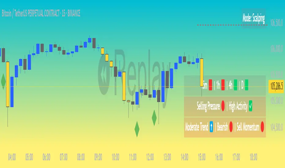
[blackcat] L2 Enhanced MACD Trend█ OVERVIEW
The Enhanced MACD Trend script combines traditional Moving Average Convergence Divergence (MACD) analysis with On-Balance Volume (OBV) insights to provide traders with a comprehensive understanding of market trends. By examining both price momentum and volume fluctuations, this tool aids in identifying potential upward or downward market transitions.
█ LOGICAL FRAMEWORK
Initially, the script prompts users to configure fundamental parameters such as the speed of moving averages. It subsequently utilizes a specialized auxiliary function named calculate_macd_obv_signals to perform intricate computations. This function calculates the discrepancy between two distinct types of moving averages (captured via MACD analysis), evaluates the direction of capital inflows and outflows within securities (using OBV), and applies smoothing techniques to mitigate undue influence from minor fluctuations. Ultimately, visual representations of these calculations are rendered on an additional chart pane for enhanced interpretability.
█ CUSTOM FUNCTIONS
Function: calculate_macd_obv_signals
• Purpose: Determines critical aspects associated with MACD and OBV.
• Parameters:
• fastLength (int): Dictates the responsiveness of the shorter Exponential Moving Average (EMA) to price variations.
• slowLength (int): Specifies the reactivity of the longer EMA.
• signalSmoothing (int): Defines the degree of smoothness applied to the divergence between EMAs.
• Functionality:
• macd_diff: Illustrates whether price increases have accelerated relative to previous levels or decelerated, providing insight into existing momentum.
• macd_signal_line: Smoothens macd_diff values, serving akin to a trailing indicator for macd_diff.
• macd_histogram: Visually accentuates disparities between macd_diff and macd_signal_line employing color-coded bars, facilitating identification of significant divergences.
• obv_signal: Represents a refined variant of short-term OBV concentrating solely on periods characterized by elevated buying interest, aiding in reduction of extraneous signals.
• moving_average_short: Analyzes recent closing prices across several sessions to corroborate burgeoning bullish or bearish tendencies.
• Returns: An array encompassing .
█ KEY POINTS AND TECHNIQUES
Advanced Features: Employs sophisticated functions including ta.ema() and ta.sma(), enabling accurate calculation of EMAs and SMAs respectively, thus enhancing precision in trend detection.
Optimization Techniques: Incorporates customizable inputs (input.int) permitting strategic adjustments alongside scrutiny of escalating or declining volumes to accurately gauge genuine sentiment shifts while discounting insignificant anomalies.
Best Practices: Maintains separation between algorithmic processes and graphical outputs, preserving organizational clarity; hence simplifying debugging efforts and future enhancements.
Unique Approaches: Integrates multifaceted assessments simultaneously – amalgamating candlestick formations and volumetric activities – offering a holistic perspective instead of reliance on singular indicators. Consequently, delivers astute recommendations grounded in diverse analytical underpinnings rather than speculative forecasts.
█ EXTENDED KNOWLEDGE AND APPLICATIONS
Potential Modifications:
1 — Implement automated alert mechanisms signaling crossover events pinpointing optimal buy/sell junctures to fine-tune timing preemptively minimizing losses proactively.
2 — Enable user customization of sensitivity criteria governing trigger intensity thereby eliminating trivial aberrations and emphasizing substantial patterns exclusively.
Application Scenarios:
Beneficial for high-frequency trading aiming to capitalize on fleeting price movements swiftly. Suitable for dynamic environments necessitating rapid responses due to frequent market volatility demanding prompt reactions. Perfect for individuals engaging in regular transactions seeking unparalleled accuracy navigating fluctuating circumstances ensuring consistent profitability amidst disturbances maintaining steady yields irrespective of upheavals.
Related Concepts:
Contemplate interactions among oscillators (such as MACD) and volume metrics detecting instances wherein they oppose each other (indicative of divergences) or concur (signaling crossovers). Profound comprehension of these interrelationships substantially refines trading strategies integrating broader economic factors, seasonal influences guiding overarching plans resulting in heightened predictive capabilities elevating trading effectiveness leveraging cumulative information transforming unprocessed statistics into actionable intelligence empowering informed decisions advancing confidently toward objectives effortlessly scaling achievements seamlessly realizing aspirations effortlessly.

Ultimate Multi-Physics Financial IndicatorThe Ultimate Multi-Physics Financial Indicator is an advanced Pine Script designed to combine various complex theories from physics, mathematics, and statistical mechanics to create a holistic, multi-dimensional approach to market analysis. Let’s break down the core concepts and how they’re applied in this script:
1. Fractal Geometry: Recursive Pattern Recognition
Purpose: This part of the script uses fractal geometry to recursively analyze price pivots (highs and lows) for detecting patterns.
Fractals: The fractalHigh and fractalLow signals represent key turning points in the market. The script goes deeper by recursively analyzing layers of pivot sequences, adding "depth" to the recognition of patterns.
Recursive Depth: It breaks down each detected pivot into smaller components, giving more nuance to market pattern recognition. This provides a broader context for how prices have behaved historically at various levels of recursion.
2. Quantum Mechanics: Adaptive Probabilistic Monte Carlo with Correlation
Purpose: This component integrates randomness (from Monte Carlo simulations) with current market behavior using correlation.
Randomness Weighted by Correlation: By generating random probabilities and weighting them based on how well the market aligns with recent trends, it creates a probabilistic signal. The random values are scaled by a correlation factor (close prices and their moving average), adding adaptive elements where randomness is adjusted by current market conditions.
3. Thermodynamics: Adaptive Efficiency Ratio (Entropy-Like Decay)
Purpose: This section uses principles from thermodynamics, where efficiency in price movement is dynamically adjusted by recent volatility and changes.
Efficiency Ratio: It calculates how efficiently the market is moving over a certain period. The "entropy decay factor" reflects how stable the market is. Higher entropy (chaos) results in lower efficiency, while stable periods maintain higher efficiency.
4. Chaos Theory: Lorenz-Driven Market Oscillation
Purpose: Instead of using a basic Average True Range (ATR) indicator, this section applies chaos theory (using a Lorenz attractor analogy) to describe complex market oscillations.
Lorenz Attractor: This models market behavior with a chaotic system that depends on the historical price changes at different time intervals. The attractor value quantifies the level of "chaos" or unpredictability in the market.
5. String Theory: Multi-Layered Dimensional Analysis of RSI and MACD
Purpose: Combines traditional indicators like the RSI (Relative Strength Index) and MACD (Moving Average Convergence Divergence) with momentum for multi-dimensional analysis.
Interaction of Layers: Each layer (RSI, MACD, and momentum) is treated as part of a multi-dimensional structure, where they influence one another. The final signal is a blended outcome of these key metrics, weighted and averaged for complexity.
6. Fluid Dynamics: Adaptive OBV (Pressure-Based)
Purpose: This section uses fluid dynamics to understand how price movement and volume create pressure over time, similar to how fluids behave under different forces.
Adaptive OBV: Traditional OBV (On-Balance Volume) is adapted by using statistical smoothing to measure the "pressure" exerted by volume over time. The result is a signal that shows where there might be building momentum or pressure in the market based on volume dynamics.
7. Recursive Synthesis of Signals
Purpose: After calculating all the individual signals (fractal, quantum, thermodynamic, chaos, string, and fluid), the script synthesizes them into one cohesive signal.
Recursive Feedback Loop: Each signal is recursively influenced by others, forming a feedback loop that allows the indicator to continuously learn from new data and self-adjust.
8. Signal Smoothing and Final Output
Purpose: To avoid noise in the output, the final combined signal is smoothed using an Exponential Moving Average (EMA), which helps stabilize the output for easier interpretation.
9. Dynamic Color Coding Based on Signal Extremes
Purpose: Visual clarity is enhanced by using color to highlight different levels of signal strength.
Color Coding: The script dynamically adjusts colors (green, orange, red) based on the strength of the final signal relative to its percentile ranking in historical data, making it easier to spot bullish, neutral, or bearish signals.
The "Ultimate Multi-Physics Financial Indicator" integrates a diverse array of scientific principles — fractal geometry, quantum mechanics, thermodynamics, chaos theory, string theory, and fluid dynamics — to provide a comprehensive market analysis tool. By combining probabilistic simulations, multi-dimensional technical indicators, and recursive feedback loops, this indicator adapts dynamically to evolving market conditions, giving traders a holistic view of market behavior across various dimensions. The result is an adaptive and flexible tool that responds to both short-term and long-term market changes

TASC 2024.08 Volume Confirmation For A Trend System█ OVERVIEW
This script demonstrates the use of volume data to validate price movements based on the techniques Buff Pelz Dormeier discusses in his "Volume Confirmation For A Trend System" article from the August 2024 edition of TASC's Traders' Tips . It presents a trend-following system implementation that utilizes a combination of three indicators: the Average Directional Index (ADX), the Trend Thrust Indicator (TTI), and the Volume Price Confirmation Indicator (VPCI).
█ CONCEPTS
In his article, Buff Pelz Dormeier recounts his search for an optimal trend-following strategy enhanced with volume data, starting with a simple system combining the ADX , MACD , and OBV indicators. Even in these early tests, the author observed that the volume confirmation from OBV notably improved trading performance. Subsequently, the author replaced OBV with his VPCI, which considers the proportional weights of volume and price, to enhance the validation of trend momentum. Lastly, the author explored the inclusion of his TTI, a modified MACD that features volume-based enhancements, as a strategy component for improved trend-following performance.
According to the author's research, the ADX+TTI+VPCI system outperformed similar strategies he tested in the article, yielding significantly higher returns and enhanced perceived reliability. Because the system's design revolves around catching pronounced trends, it performs best with a portfolio of individual stocks. The author applies the system in the article by allocating 5% of the equity to long positions in S&P 500 components that meet the ADX+TTI+VPCI entry criteria (see the Calculations section below for details). He uses the proceeds from closing positions to enter new positions in other stocks meeting the screening criteria, holding any excess proceeds in cash.
█ CALCULATIONS
The TTI is similar to the MACD. Its calculation entails the following steps:
Calculate fast (short-term) and slow (long-term) volume-weighted moving averages (VWMAs).
Compute the volume multiple (VM) as the square of the ratio of the fast VWMA to the slow VWMA.
Adjust these averages by multiplying the fast VWMA by the VM and dividing the slow VWMA by the VM.
Calculate the difference between the adjusted VWMAs to determine the TTI value, and take the average of that series to determine the signal line value.
The VPCI utilizes differences and ratios between VWMAs and corresponding simple moving averages (SMAs) to provide an alternative volume-price confirmation tool. Its calculation is as follows:
Subtract the slow SMA from the VWMA of the same length to calculate the volume-price confirmation/contradiction (VPC) value.
Divide the fast VWMA by the corresponding fast SMA to determine the volume-price ratio (VPR).
Divide the short-term VWMA by the long-term VWMA to calculate the VM.
Compute the VPCI as the product of the VPC, VPR, and VM values.
The long entry criteria of the ADX+TTI+VPCI system are as follows:
The ADX is above 30.
The TTI crosses above its signal line.
The VPCI is above 0, confirming the trend.
Signals to close positions occur when the VPCI is below 0, indicating a contradiction .
NOTE: Unlike in the article, this script applies the ADX+TTI+VPCI system to one stock at a time , not a portfolio of S&P 500 constituents.
█ DISCLAIMER
This strategy script educates users on the trading system outlined by the TASC article. By default, it uses 10% of equity as the order size and a slippage amount of 5 ticks. Traders should adjust these settings and the commission amount when using this script.

The On Balance Volume & Accumulation Distribution RibbonMedic trades using "Smart Money Concepts", and Medic's system revolves around the one taught by MentFX (i.e. Structure, Supply/ Demand Zone , and Confirmation). While this system per se doesn't require the use of a volume indicator, Medic has come to respect the OBV and Accumulation / Distribution .
The OBV Ribbon is available in many a shape and form, but Medic wanted something more responsive, and the OBVAD is just that.
This ribbon works across all time frames, and allows users to visualize what is happening behind the scenes of The Trigger indicator.
The Ribbon applies 11 DEMA of different periods to the cumulative sum of SpaceTrader's OBV/AD formula: volume*(close-open)/( high-low )*hlc3.
The Ribbon is able to identify the general trend, and changes into a blu ein an uptrend, and purple in a downtrend, and also potential reversals by means of divergences.

Profile Any Indicator [Kioseff Trading]Create a visible-range profile for almost any indicator!
Hello!
This script "Profile Any Indicator" allows you to create a visible-range profile for *almost* any indicator hosted on TradingView.
Therefore, the only requirement:
1. Indicator must have a retrievable plot value.
Should your indicator have a retrievable plot value (most indicators do), you can use this script to create a visible-range profile of its values!
Consequently, the profile's always oriented to the left-most or right-most side of your chart - updating as you scroll left or right.
The image above shows me using the indicator to create a profile for MACD. I am largely zoomed out and the profile has adjusted to chart orientation.
Let's zoom in and see what happens!
Voila!
The indicator adjusted to my chart positioning and created a new visible-range profile! No manual adjustments are required (:
Instructions
1. Load the indicator you'd like to profile on the chart.
The image above shows me applying the OBV indicator to the chart. Additionally, the "Profile Any Indicator" script is also loaded on the chart, instructing me to add an indicator to its settings.
2. From the settings for "Profile Any indicator", locate the "Indicator" setting and select the indicator you would like to profile.
The image above shows me selecting the OBV indicator in the settings for "Profile Any Indicator".
Once steps 1 and 2 are complete you'll have a visible-range profile for the selected indicator on your chart!
The image above shows the completion of the process.
3. Merge the indicator pane or select to plot the selected indicator in the current pane.
From here, you can select to plot the value of the selected indicator in the current pane or merge the selected indicator's pane (which must stay on the chart) with the pane designated to the "Profile Any Indicator" script.
The image above shows the two panes merged.
The image above shows the two panes separate. Alternatively, in the settings for "Profile Any Indicator", I selected to plot OBV in its pane.
You can select to populate the visible-range profile on the right of the chart!
Additionally, you can modify the POC line, value area %, and, essentially, any parameter you'd find for a volume-profile-like indicator!
Thanks for checking this out (: