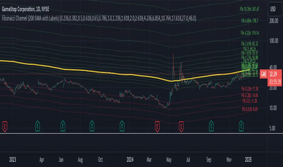
Fibonacci Channel Standard Deviation levels based off 200MAThis script dynamically combines Fibonacci levels with the 200-period simple moving average (SMA), offering a powerful tool for identifying high-probability support and resistance zones. By adjusting to the changing 200 SMA, the script remains relevant across different market phases.
Key Features:
Dynamic Fibonacci Levels:
The script automatically calculates Fibonacci retracements and extensions relative to the 200 SMA.
These levels adapt to market trends, offering more relevant zones compared to static Fibonacci tools.
Support and Resistance Zones:
In uptrends, price often respects retracement levels above the 200 SMA (e.g., 38.2%, 50%, 61.8%).
In downtrends, price may interact with retracements and extensions below the 200 SMA (e.g., 23.6%, 1.618).
Customizable Confluence Zones:
Key levels such as the golden pocket (61.8%–65%) are highlighted as high-probability zones for reversals or continuations.
Extensions (e.g., 1.618) can serve as profit targets or bearish continuation points.
Practical Applications:
Identifying Reversal Zones:
Look for confluence between Fibonacci levels and the 200 SMA to identify potential reversal points.
Example: A pullback to the 61.8%–65% golden pocket near the 200 SMA often signals a bullish reversal.
Trend Confirmation:
In uptrends, price respecting Fibonacci retracements above the 200 SMA (e.g., 38.2%, 50%) confirms strength.
Use Fibonacci extensions (e.g., 1.618) as profit targets during strong trends.
Dynamic Risk Management:
Place stop-losses just below key Fibonacci retracement levels near the 200 SMA to minimize risk.
Bearish Scenarios:
Below the 200 SMA, Fibonacci retracements and extensions act as resistance levels and bearish targets.
How to Use:
Volume Confirmation: Watch for volume spikes near Fibonacci levels to confirm support or resistance.
Price Action: Combine with candlestick patterns (e.g., engulfing candles, pin bars) for precise entries.
Trend Indicators: Use in conjunction with shorter moving averages or RSI to confirm market direction.
Example Setup:
Scenario: Price retraces to the 61.8% Fibonacci level while holding above the 200 SMA.
Confirmation: Volume spikes, and a bullish engulfing candle forms.
Action: Enter long with a stop-loss just below the 200 SMA and target extensions like 1.618.
Key Takeaways:
The 200 SMA serves as a reliable long-term trend anchor.
Fibonacci retracements and extensions provide dynamic zones for trade entries, exits, and risk management.
Combining this tool with volume, price action, or other indicators enhances its effectiveness.
Cerca negli script per "TAKE"
Milvetti_TraderPost_LibraryLibrary "Milvetti_TraderPost_Library"
This library has methods that provide practical signal transmission for traderpost.Developed By Milvetti
cancelOrders(symbol)
This method generates a signal in JSON format that cancels all orders for the specified pair. (If you want to cancel stop loss and takeprofit orders together, use the “exitOrder” method.
Parameters:
symbol (string)
exitOrders(symbol)
This method generates a signal in JSON format that close all orders for the specified pair.
Parameters:
symbol (string)
createOrder(ticker, positionType, orderType, entryPrice, signalPrice, qtyType, qty, stopLoss, stopType, stopValue, takeProfit, profitType, profitValue, timeInForce)
This function is designed to send buy or sell orders to traderpost. It can create customized orders by flexibly specifying parameters such as order type, position type, entry price, quantity calculation method, stop-loss, and take-profit. The purpose of the function is to consolidate all necessary details for opening a position into a single structure and present it as a structured JSON output. This format can be sent to trading platforms via webhooks.
Parameters:
ticker (string) : The ticker symbol of the instrument. Default value is the current chart's ticker (syminfo.ticker).
positionType (string) : Determines the type of order (e.g., "long" or "buy" for buying and "short" or "sell" for selling).
orderType (string) : Defines the order type for execution. Options: "market", "limit", "stop". Default is "market"
entryPrice (float) : The price level for entry orders. Only applicable for limit or stop orders. Default is 0 (market orders ignore this).
signalPrice (float) : Optional. Only necessary when using relative take profit or stop losses, and the broker does not support fetching quotes to perform the calculation. Default is 0
qtyType (string) : Determines how the order quantity is calculated. Options: "fixed_quantity", "dollar_amount", "percent_of_equity", "percent_of_position".
qty (float) : Quantity value. Can represent units of shares/contracts or a dollar amount, depending on qtyType.
stopLoss (bool) : Enable or disable stop-loss functionality. Set to `true` to activate.
stopType (string) : Specifies the stop-loss calculation type. Options: percent, "amount", "stopPrice", "trailPercent", "trailAmount". Default is "stopPrice"
stopValue (float) : Stop-loss value based on stopType. Can be a percentage, dollar amount, or a specific stop price. Default is "stopPrice"
takeProfit (bool) : Enable or disable take-profit functionality. Set to `true` to activate.
profitType (string) : Specifies the take-profit calculation type. Options: "percent", "amount", "limitPrice". Default is "limitPrice"
profitValue (float) : Take-profit value based on profitType. Can be a percentage, dollar amount, or a specific limit price. Default is 0
timeInForce (string) : The time in force for your order. Options: day, gtc, opg, cls, ioc and fok
Returns: Return result in Json format.
addTsl(symbol, stopType, stopValue, price)
This method adds trailing stop loss to the current position. “Price” is the trailing stop loss starting level. You can leave price blank if you want it to start immediately
Parameters:
symbol (string)
stopType (string) : Specifies the trailing stoploss calculation type. Options: "trailPercent", "trailAmount".
stopValue (float) : Stop-loss value based on stopType. Can be a percentage, dollar amount.
price (float) : The trailing stop loss starting level. You can leave price blank if you want it to start immediately. Default is current price.
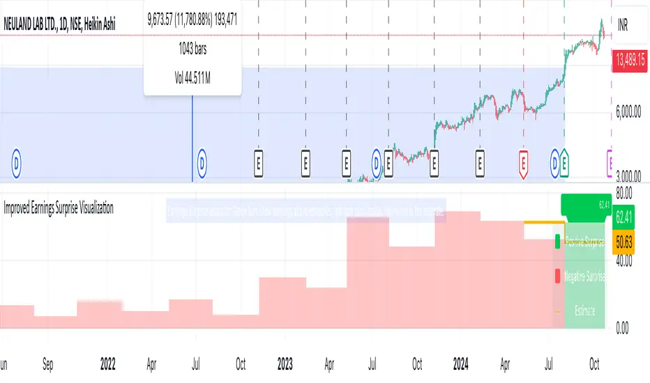
Earnings Surprise Indicator (Post-Earnings Announcement Drift)What It Does:
- Displays a company's actual earnings vs. analysts' estimates over time
- Shows "earnings surprises" - when actual results beat or miss expectations
- Helps identify trends in a company's financial performance
How It Works:
- Green bars: Positive surprise (earnings beat estimates)
- Red bars: Negative surprise (earnings missed estimates)
- Yellow line: Analysts' earnings estimates
Correlation with Post Earnings Announcement Drift (PEAD): PEAD is the tendency for a stock's price to drift in the direction of an earnings surprise for several weeks or months after the announcement.
Why It Matters:
- Positive surprises often lead to upward price drift
- Negative surprises often lead to downward price drift
- This drift can create trading opportunities
How to Use It:
1. Spot Trends:
- Consistent beats may indicate strong company performance
- Consistent misses may signal underlying issues
2. Gauge Market Expectations:
- Large surprises may lead to significant price movements
3. Timing Decisions:
- Consider long positions after positive surprises
- Consider short positions or exits after negative surprises
4. Risk Management:
- Be cautious of reversal if the drift seems excessive
- Use in conjunction with other technical and fundamental analysis
Key Takeaways:
- Earnings surprises can be fundamental-leading indicators of future stock performance, especially when correlated with analyst projections
- PEAD suggests that markets often underreact to earnings news initially
- This indicator helps visualize the magnitude and direction of surprises
- It can be a valuable tool for timing entry and exit points in trades
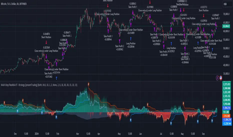
Multi-Step FlexiMA - Strategy [presentTrading]It's time to come back! hope I can not to be busy for a while.
█ Introduction and How It Is Different
The FlexiMA Variance Tracker is a unique trading strategy that calculates a series of deviations between the price (or another indicator source) and a variable-length moving average (MA). Unlike traditional strategies that use fixed-length moving averages, the length of the MA in this system varies within a defined range. The length changes dynamically based on a starting factor and an increment factor, creating a more adaptive approach to market conditions.
This strategy integrates Multi-Step Take Profit (TP) levels, allowing for partial exits at predefined price increments. It enables traders to secure profits at different stages of a trend, making it ideal for volatile markets where taking full profits at once might lead to missed opportunities if the trend continues.
BTCUSD 6hr Performance
█ Strategy, How It Works: Detailed Explanation
🔶 FlexiMA Concept
The FlexiMA (Flexible Moving Average) is at the heart of this strategy. Unlike traditional MA-based strategies where the MA length is fixed (e.g., a 50-period SMA), the FlexiMA varies its length with each iteration. This is done using a **starting factor** and an **increment factor**.
The formula for the moving average length at each iteration \(i\) is:
`MA_length_i = indicator_length * (starting_factor + i * increment_factor)`
Where:
- `indicator_length` is the user-defined base length.
- `starting_factor` is the initial multiplier of the base length.
- `increment_factor` increases the multiplier in each iteration.
Each iteration applies a **simple moving average** (SMA) to the chosen **indicator source** (e.g., HLC3) with a different length based on the above formula. The deviation between the current price and the moving average is then calculated as follows:
`deviation_i = price_current - MA_i`
These deviations are normalized using one of the following methods:
- **Max-Min normalization**:
`normalized_i = (deviation_i - min(deviations)) / range(deviations)`
- **Absolute Sum normalization**:
`normalized_i = deviation_i / sum(|deviation_i|)`
The **median** and **standard deviation (stdev)** of the normalized deviations are then calculated as follows:
`median = median(normalized deviations)`
For the standard deviation:
`stdev = sqrt((1/(N-1)) * sum((normalized_i - mean)^2))`
These values are plotted to provide a clear indication of how the price is deviating from its variable-length moving averages.
For more detail:
🔶 Multi-Step Take Profit
This strategy uses a multi-step take profit system, allowing for exits at different stages of a trade based on the percentage of price movement. Three take-profit levels are defined:
- Take Profit Level 1 (TP1): A small, quick profit level (e.g., 2%).
- Take Profit Level 2 (TP2): A medium-level profit target (e.g., 8%).
- Take Profit Level 3 (TP3): A larger, more ambitious target (e.g., 18%).
At each level, a corresponding percentage of the trade is exited:
- TP Percent 1: E.g., 30% of the position.
- TP Percent 2: E.g., 20% of the position.
- TP Percent 3: E.g., 15% of the position.
This approach ensures that profits are locked in progressively, reducing the risk of market reversals wiping out potential gains.
Local
🔶 Trade Entry and Exit Conditions
The entry and exit signals are determined by the interaction between the **SuperTrend Polyfactor Oscillator** and the **median** value of the normalized deviations:
- Long entry: The SuperTrend turns bearish, and the median value of the deviations is positive.
- Short entry: The SuperTrend turns bullish, and the median value is negative.
Similarly, trades are exited when the SuperTrend flips direction.
* The SuperTrend Toolkit is made by @EliCobra
█ Trade Direction
The strategy allows users to specify the desired trade direction:
- Long: Only long positions will be taken.
- Short: Only short positions will be taken.
- Both: Both long and short positions are allowed based on the conditions.
This flexibility allows the strategy to adapt to different market conditions and trading styles, whether you're looking to buy low and sell high, or sell high and buy low.
█ Usage
This strategy can be applied across various asset classes, including stocks, cryptocurrencies, and forex. The primary use case is to take advantage of market volatility by using a flexible moving average and multiple take-profit levels to capture profits incrementally as the market moves in your favor.
How to Use:
1. Configure the Inputs: Start by adjusting the **Indicator Length**, **Starting Factor**, and **Increment Factor** to suit your chosen asset. The defaults work well for most markets, but fine-tuning them can improve performance.
2. Set the Take Profit Levels: Adjust the three **TP levels** and their corresponding **percentages** based on your risk tolerance and the expected volatility of the market.
3. Monitor the Strategy: The SuperTrend and the FlexiMA variance tracker will provide entry and exit signals, automatically managing the positions and taking profits at the pre-set levels.
█ Default Settings
The default settings for the strategy are configured to provide a balanced approach that works across different market conditions:
Indicator Length (10):
This controls the base length for the moving average. A lower length makes the moving average more responsive to price changes, while a higher length smooths out fluctuations, making the strategy less sensitive to short-term price movements.
Starting Factor (1.0):
This determines the initial multiplier applied to the moving average length. A higher starting factor will increase the average length, making it slower to react to price changes.
Increment Factor (1.0):
This increases the moving average length in each iteration. A larger increment factor creates a wider range of moving average lengths, allowing the strategy to track both short-term and long-term trends simultaneously.
Normalization Method ('None'):
Three methods of normalization can be applied to the deviations:
- None: No normalization applied, using raw deviations.
- Max-Min: Normalizes based on the range between the maximum and minimum deviations.
- Absolute Sum: Normalizes based on the total sum of absolute deviations.
Take Profit Levels:
- TP1 (2%): A quick exit to capture small price movements.
- TP2 (8%): A medium-term profit target for stronger trends.
- TP3 (18%): A long-term target for strong price moves.
Take Profit Percentages:
- TP Percent 1 (30%): Exits 30% of the position at TP1.
- TP Percent 2 (20%): Exits 20% of the position at TP2.
- TP Percent 3 (15%): Exits 15% of the position at TP3.
Effect of Variables on Performance:
- Short Indicator Lengths: More responsive to price changes but prone to false signals.
- Higher Starting Factor: Slows down the response, useful for longer-term trend following.
- Higher Increment Factor: Widens the variability in moving average lengths, making the strategy adapt to both short-term and long-term price trends.
- Aggressive Take Profit Levels: Allows for quick profit-taking in volatile markets but may exit positions prematurely in strong trends.
The default configuration offers a moderate balance between short-term responsiveness and long-term trend capturing, suitable for most traders. However, users can adjust these variables to optimize performance based on market conditions and personal preferences.
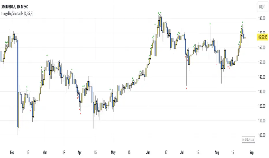
Longable/ShortableThis indicator advises intraday traders which direction NOT to take trades in, based on recent action in the daily chart. Works on any timeframe.
This is not a buy/sell indicator - it is a FILTER that is meant to SUPPRESS trades you may have wanted to take. Like a Daily Bias, but with a neutral position (no bias).
The indicator shows when NOT to take longs and when NOT to take shorts.
So you need an existing strategy to combine this with.
By default, the last 3 days are taken into account (smoothing=3). Change the threshold to get fewer or more warning signals.
The symbols are very simple:
Green triangle = Longs only
Red triangle = Shorts only
(Each signal is valid for the next candle. After that it expires.)
The current bias is also shown in the bottom right corner.
How it works: We look at which parts of the last candle overlap with the current one. When the new candle's low is far above the last candle's low, it is an indication not to go short. Similarly, when the new candle's high is far below the last candle's high, it is an indication not to go long.
For each direction, we calculate this as a percentage value (what percentage of the last candle is not overlapping the new one), smooth the value and give a signal when we are above the set threshold.
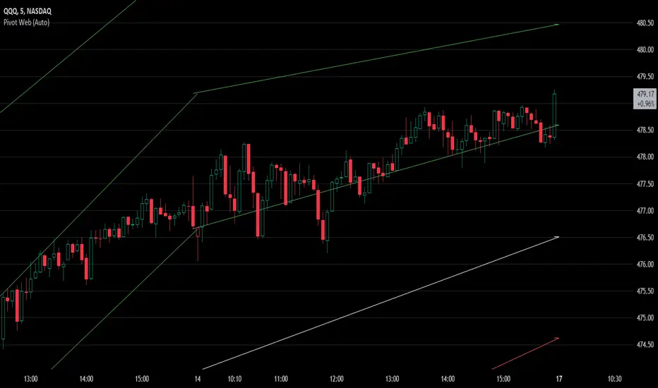
Pivot WebThe Pivot Web is a prototype with its base derived from TradingView's standard pivot point indicator plus inspiration from LuxAlgo's trendline work alongside my own observations/experiences.
The theory is that there's legitimacy, from a technical standpoint, pivot point calculations are an adequate gauge of momentum and sentiment because the same math was used under pressure by floor traders themselves. That calculation is centered on the average of high, low, and closing prices. This indicator creates trendlines connecting the last pivot, support, and resistance levels to the current ones. A dynamic visual cue could make it easier to assess if the price will continue or reverse the current trajectory. This method also shows us an excellent visual for volatility.
Key Takeaways:
This indicator draws new dynamic trendlines.
These new trendlines connect the past and present pivot point levels based on the timeframe you select.
Shorter timeframes = More trendlines
Price adherence to the path of these lines may offer insight for trading.
Lastly, note the first set of data in each new timeframe displays the current original pivot point levels along with the trendlines attached to their ending point. Most of the time this indicator leaves room by briefly highlighting the original static levels with all levels also being optional displays. Also note that a more stable asset may not require the outermost support and resistance levels. Like most time series analysis tools, the Pivot Web requires current data to function properly.
"Nature is pleased with simplicity, and nature is no dummy."
One Setup for Life ICTGuided by ICT tutoring, I create this versatile 'One Trading Set Up For Life' indicator
This indicator shows a different way of viewing the "Highs and Lows" of Previous Sessions, drawing from the current day until 09:30 AM, the time at which the Highs and Lows of the previous day's sessions can be taken into consideration for a Reversal or for a Take profit.
Levels tested after 9.30am will be blocked so you have a good and clear view of the levels affected
Timing Session =
London: 02:00 to 05:00
New York: 9.30am to 12.30pm
Lunch: 12.30pm to 1pm
PM Session: 1.30pm to 4pm
The user has the possibility to:
- Choose to view sessions or not
- Choose to show levels from previous sessions
- Choose to show today's session levels
- Choose between 08:30 and 09:30 the starting time for the Liquidity taken
- Choose to view High and Low only from the previous day
- See both the name of the Sessions and the price of the levels
The indicator must be used as ICT shows in its concepts, the indicator takes into consideration both previous sessions and today's sessions, and the session levels can be used both for a reversal and for a possible Take Profit like the example here under
Reversal =
Possible Take Profit =
If something is not clear, comment below and I will reply as soon as possible.

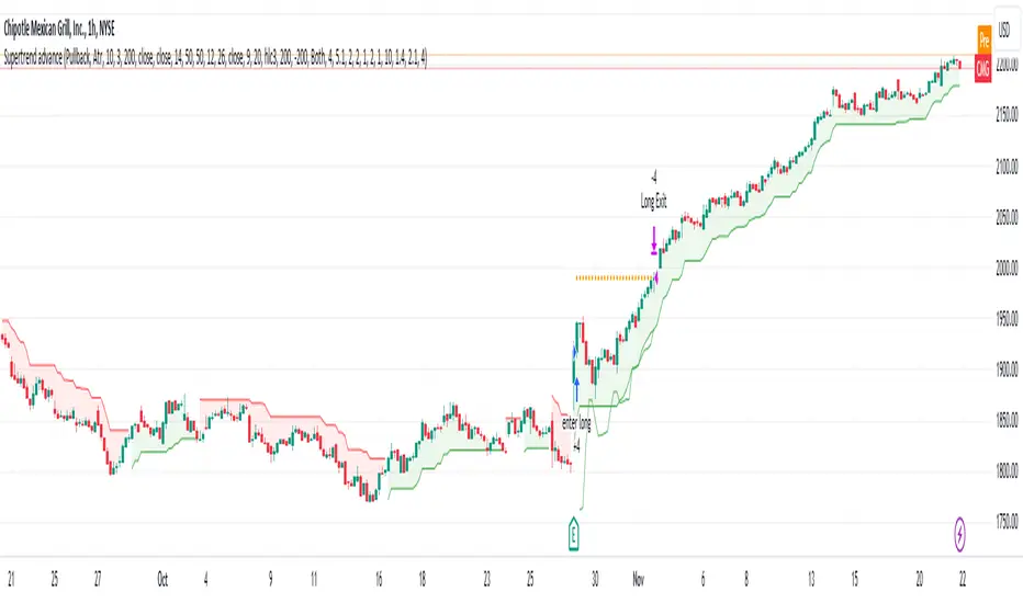
Supertrend Advance Pullback StrategyHandbook for the Supertrend Advance Strategy
1. Introduction
Purpose of the Handbook:
The main purpose of this handbook is to serve as a comprehensive guide for traders and investors who are looking to explore and harness the potential of the Supertrend Advance Strategy. In the rapidly changing financial market, having the right tools and strategies at one's disposal is crucial. Whether you're a beginner hoping to dive into the world of trading or a seasoned investor aiming to optimize and diversify your portfolio, this handbook offers the insights and methodologies you need. By the end of this guide, readers should have a clear understanding of how the Supertrend Advance Strategy works, its benefits, potential pitfalls, and practical application in various trading scenarios.
Overview of the Supertrend Advance Pullback Strategy:
At its core, the Supertrend Advance Strategy is an evolution of the popular Supertrend Indicator. Designed to generate buy and sell signals in trending markets, the Supertrend Indicator has been a favorite tool for many traders around the world. The Advance Strategy, however, builds upon this foundation by introducing enhanced mechanisms, filters, and methodologies to increase precision and reduce false signals.
1. Basic Concept:
The Supertrend Advance Strategy relies on a combination of price action and volatility to determine the potential trend direction. By assessing the average true range (ATR) in conjunction with specific price points, this strategy aims to highlight the potential starting and ending points of market trends.
2. Methodology:
Unlike the traditional Supertrend Indicator, which primarily focuses on closing prices and ATR, the Advance Strategy integrates other critical market variables, such as volume, momentum oscillators, and perhaps even fundamental data, to validate its signals. This multidimensional approach ensures that the generated signals are more reliable and are less prone to market noise.
3. Benefits:
One of the main benefits of the Supertrend Advance Strategy is its ability to filter out false breakouts and minor price fluctuations, which can often lead to premature exits or entries in the market. By waiting for a confluence of factors to align, traders using this advanced strategy can increase their chances of entering or exiting trades at optimal points.
4. Practical Applications:
The Supertrend Advance Strategy can be applied across various timeframes, from intraday trading to swing trading and even long-term investment scenarios. Furthermore, its flexible nature allows it to be tailored to different asset classes, be it stocks, commodities, forex, or cryptocurrencies.
In the subsequent sections of this handbook, we will delve deeper into the intricacies of this strategy, offering step-by-step guidelines on its application, case studies, and tips for maximizing its efficacy in the volatile world of trading.
As you journey through this handbook, we encourage you to approach the Supertrend Advance Strategy with an open mind, testing and tweaking it as per your personal trading style and risk appetite. The ultimate goal is not just to provide you with a new tool but to empower you with a holistic strategy that can enhance your trading endeavors.
2. Getting Started
Navigating the financial markets can be a daunting task without the right tools. This section is dedicated to helping you set up the Supertrend Advance Strategy on one of the most popular charting platforms, TradingView. By following the steps below, you'll be able to integrate this strategy into your charts and start leveraging its insights in no time.
Setting up on TradingView:
TradingView is a web-based platform that offers a wide range of charting tools, social networking, and market data. Before you can apply the Supertrend Advance Strategy, you'll first need a TradingView account. If you haven't set one up yet, here's how:
1. Account Creation:
• Visit TradingView's official website.
• Click on the "Join for free" or "Sign up" button.
• Follow the registration process, providing the necessary details and setting up your login credentials.
2. Navigating the Dashboard:
• Once logged in, you'll be taken to your dashboard. Here, you'll see a variety of tools, including watchlists, alerts, and the main charting window.
• To begin charting, type in the name or ticker of the asset you're interested in the search bar at the top.
3. Configuring Chart Settings:
• Before integrating the Supertrend Advance Strategy, familiarize yourself with the chart settings. This can be accessed by clicking the 'gear' icon on the top right of the chart window.
• Adjust the chart type, time intervals, and other display settings to your preference.
Integrating the Strategy into a Chart:
Now that you're set up on TradingView, it's time to integrate the Supertrend Advance Strategy.
1. Accessing the Pine Script Editor:
• Located at the top-center of your screen, you'll find the "Pine Editor" tab. Click on it.
• This is where custom strategies and indicators are scripted or imported.
2. Loading the Supertrend Advance Strategy Script:
• Depending on whether you have the script or need to find it, there are two paths:
• If you have the script: Copy the Supertrend Advance Strategy script, and then paste it into the Pine Editor.
• If searching for the script: Click on the “Indicators” icon (looks like a flame) at the top of your screen, and then type “Supertrend Advance Strategy” in the search bar. If available, it will show up in the list. Simply click to add it to your chart.
3. Applying the Strategy:
• After pasting or selecting the Supertrend Advance Strategy in the Pine Editor, click on the “Add to Chart” button located at the top of the editor. This will overlay the strategy onto your main chart window.
4. Configuring Strategy Settings:
• Once the strategy is on your chart, you'll notice a small settings ('gear') icon next to its name in the top-left of the chart window. Click on this to access settings.
• Here, you can adjust various parameters of the Supertrend Advance Strategy to better fit your trading style or the specific asset you're analyzing.
5. Interpreting Signals:
• With the strategy applied, you'll now see buy/sell signals represented on your chart. Take time to familiarize yourself with how these look and behave over various timeframes and market conditions.
3. Strategy Overview
What is the Supertrend Advance Strategy?
The Supertrend Advance Strategy is a refined version of the classic Supertrend Indicator, which was developed to aid traders in spotting market trends. The strategy utilizes a combination of data points, including average true range (ATR) and price momentum, to generate buy and sell signals.
In essence, the Supertrend Advance Strategy can be visualized as a line that moves with the price. When the price is above the Supertrend line, it indicates an uptrend and suggests a potential buy position. Conversely, when the price is below the Supertrend line, it hints at a downtrend, suggesting a potential selling point.
Strategy Goals and Objectives:
1. Trend Identification: At the core of the Supertrend Advance Strategy is the goal to efficiently and consistently identify prevailing market trends. By recognizing these trends, traders can position themselves to capitalize on price movements in their favor.
2. Reducing Noise: Financial markets are often inundated with 'noise' - short-term price fluctuations that can mislead traders. The Supertrend Advance Strategy aims to filter out this noise, allowing for clearer decision-making.
3. Enhancing Risk Management: With clear buy and sell signals, traders can set more precise stop-loss and take-profit points. This leads to better risk management and potentially improved profitability.
4. Versatility: While primarily used for trend identification, the strategy can be integrated with other technical tools and indicators to create a comprehensive trading system.
Type of Assets/Markets to Apply the Strategy:
1. Equities: The Supertrend Advance Strategy is highly popular among stock traders. Its ability to capture long-term trends makes it particularly useful for those trading individual stocks or equity indices.
2. Forex: Given the 24-hour nature of the Forex market and its propensity for trends, the Supertrend Advance Strategy is a valuable tool for currency traders.
3. Commodities: Whether it's gold, oil, or agricultural products, commodities often move in extended trends. The strategy can help in identifying and capitalizing on these movements.
4. Cryptocurrencies: The volatile nature of cryptocurrencies means they can have pronounced trends. The Supertrend Advance Strategy can aid crypto traders in navigating these often tumultuous waters.
5. Futures & Options: Traders and investors in derivative markets can utilize the strategy to make more informed decisions about contract entries and exits.
It's important to note that while the Supertrend Advance Strategy can be applied across various assets and markets, its effectiveness might vary based on market conditions, timeframe, and the specific characteristics of the asset in question. As always, it's recommended to use the strategy in conjunction with other analytical tools and to backtest its effectiveness in specific scenarios before committing to trades.
4. Input Settings
Understanding and correctly configuring input settings is crucial for optimizing the Supertrend Advance Strategy for any specific market or asset. These settings, when tweaked correctly, can drastically impact the strategy's performance.
Grouping Inputs:
Before diving into individual input settings, it's important to group similar inputs. Grouping can simplify the user interface, making it easier to adjust settings related to a specific function or indicator.
Strategy Choice:
This input allows traders to select from various strategies that incorporate the Supertrend indicator. Options might include "Supertrend with RSI," "Supertrend with MACD," etc. By choosing a strategy, the associated input settings for that strategy become available.
Supertrend Settings:
1. Multiplier: Typically, a default value of 3 is used. This multiplier is used in the ATR calculation. Increasing it makes the Supertrend line further from prices, while decreasing it brings the line closer.
2. Period: The number of bars used in the ATR calculation. A common default is 7.
EMA Settings (Exponential Moving Average):
1. Period: Defines the number of previous bars used to calculate the EMA. Common periods are 9, 21, 50, and 200.
2. Source: Allows traders to choose which price (Open, Close, High, Low) to use in the EMA calculation.
RSI Settings (Relative Strength Index):
1. Length: Determines how many periods are used for RSI calculation. The standard setting is 14.
2. Overbought Level: The threshold at which the asset is considered overbought, typically set at 70.
3. Oversold Level: The threshold at which the asset is considered oversold, often at 30.
MACD Settings (Moving Average Convergence Divergence):
1. Short Period: The shorter EMA, usually set to 12.
2. Long Period: The longer EMA, commonly set to 26.
3. Signal Period: Defines the EMA of the MACD line, typically set at 9.
CCI Settings (Commodity Channel Index):
1. Period: The number of bars used in the CCI calculation, often set to 20.
2. Overbought Level: Typically set at +100, denoting overbought conditions.
3. Oversold Level: Usually set at -100, indicating oversold conditions.
SL/TP Settings (Stop Loss/Take Profit):
1. SL Multiplier: Defines the multiplier for the average true range (ATR) to set the stop loss.
2. TP Multiplier: Defines the multiplier for the average true range (ATR) to set the take profit.
Filtering Conditions:
This section allows traders to set conditions to filter out certain signals. For example, one might only want to take buy signals when the RSI is below 30, ensuring they buy during oversold conditions.
Trade Direction and Backtest Period:
1. Trade Direction: Allows traders to specify whether they want to take long trades, short trades, or both.
2. Backtest Period: Specifies the time range for backtesting the strategy. Traders can choose from options like 'Last 6 months,' 'Last 1 year,' etc.
It's essential to remember that while default settings are provided for many of these tools, optimal settings can vary based on the market, timeframe, and trading style. Always backtest new settings on historical data to gauge their potential efficacy.
5. Understanding Strategy Conditions
Developing an understanding of the conditions set within a trading strategy is essential for traders to maximize its potential. Here, we delve deep into the logic behind these conditions, using the Supertrend Advance Strategy as our focal point.
Basic Logic Behind Conditions:
Every strategy is built around a set of conditions that provide buy or sell signals. The conditions are based on mathematical or statistical methods and are rooted in the study of historical price data. The fundamental idea is to recognize patterns or behaviors that have been profitable in the past and might be profitable in the future.
Buy and Sell Conditions:
1. Buy Conditions: Usually formulated around bullish signals or indicators suggesting upward price momentum.
2. Sell Conditions: Centered on bearish signals or indicators indicating downward price momentum.
Simple Strategy:
The simple strategy could involve using just the Supertrend indicator. Here:
• Buy: When price closes above the Supertrend line.
• Sell: When price closes below the Supertrend line.
Pullback Strategy:
This strategy capitalizes on price retracements:
• Buy: When the price retraces to the Supertrend line after a bullish signal and is supported by another bullish indicator.
• Sell: When the price retraces to the Supertrend line after a bearish signal and is confirmed by another bearish indicator.
Indicators Used:
EMA (Exponential Moving Average):
• Logic: EMA gives more weight to recent prices, making it more responsive to current price movements. A shorter-period EMA crossing above a longer-period EMA can be a bullish sign, while the opposite is bearish.
RSI (Relative Strength Index):
• Logic: RSI measures the magnitude of recent price changes to analyze overbought or oversold conditions. Values above 70 are typically considered overbought, and values below 30 are considered oversold.
MACD (Moving Average Convergence Divergence):
• Logic: MACD assesses the relationship between two EMAs of a security’s price. The MACD line crossing above the signal line can be a bullish signal, while crossing below can be bearish.
CCI (Commodity Channel Index):
• Logic: CCI compares a security's average price change with its average price variation. A CCI value above +100 may mean the price is overbought, while below -100 might signify an oversold condition.
And others...
As the strategy expands or contracts, more indicators might be added or removed. The crucial point is to understand the core logic behind each, ensuring they align with the strategy's objectives.
Logic Behind Each Indicator:
1. EMA: Emphasizes recent price movements; provides dynamic support and resistance levels.
2. RSI: Indicates overbought and oversold conditions based on recent price changes.
3. MACD: Showcases momentum and direction of a trend by comparing two EMAs.
4. CCI: Measures the difference between a security's price change and its average price change.
Understanding strategy conditions is not just about knowing when to buy or sell but also about comprehending the underlying market dynamics that those conditions represent. As you familiarize yourself with each condition and indicator, you'll be better prepared to adapt and evolve with the ever-changing financial markets.
6. Trade Execution and Management
Trade execution and management are crucial aspects of any trading strategy. Efficient execution can significantly impact profitability, while effective management can preserve capital during adverse market conditions. In this section, we'll explore the nuances of position entry, exit strategies, and various Stop Loss (SL) and Take Profit (TP) methodologies within the Supertrend Advance Strategy.
Position Entry:
Effective trade entry revolves around:
1. Timing: Enter at a point where the risk-reward ratio is favorable. This often corresponds to confirmatory signals from multiple indicators.
2. Volume Analysis: Ensure there's adequate volume to support the movement. Volume can validate the strength of a signal.
3. Confirmation: Use multiple indicators or chart patterns to confirm the entry point. For instance, a buy signal from the Supertrend indicator can be confirmed with a bullish MACD crossover.
Position Exit Strategies:
A successful exit strategy will lock in profits and minimize losses. Here are some strategies:
1. Fixed Time Exit: Exiting after a predetermined period.
2. Percentage-based Profit Target: Exiting after a certain percentage gain.
3. Indicator-based Exit: Exiting when an indicator gives an opposing signal.
Percentage-based SL/TP:
• Stop Loss (SL): Set a fixed percentage below the entry price to limit potential losses.
• Example: A 2% SL on an entry at $100 would trigger a sell at $98.
• Take Profit (TP): Set a fixed percentage above the entry price to lock in gains.
• Example: A 5% TP on an entry at $100 would trigger a sell at $105.
Supertrend-based SL/TP:
• Stop Loss (SL): Position the SL at the Supertrend line. If the price breaches this line, it could indicate a trend reversal.
• Take Profit (TP): One could set the TP at a point where the Supertrend line flattens or turns, indicating a possible slowdown in momentum.
Swing high/low-based SL/TP:
• Stop Loss (SL): For a long position, set the SL just below the recent swing low. For a short position, set it just above the recent swing high.
• Take Profit (TP): For a long position, set the TP near a recent swing high or resistance. For a short position, near a swing low or support.
And other methods...
1. Trailing Stop Loss: This dynamic SL adjusts with the price movement, locking in profits as the trade moves in your favor.
2. Multiple Take Profits: Divide the position into segments and set multiple TP levels, securing profits in stages.
3. Opposite Signal Exit: Exit when another reliable indicator gives an opposite signal.
Trade execution and management are as much an art as they are a science. They require a blend of analytical skill, discipline, and intuition. Regularly reviewing and refining your strategies, especially in light of changing market conditions, is crucial to maintaining consistent trading performance.
7. Visual Representations
Visual tools are essential for traders, as they simplify complex data into an easily interpretable format. Properly analyzing and understanding the plots on a chart can provide actionable insights and a more intuitive grasp of market conditions. In this section, we’ll delve into various visual representations used in the Supertrend Advance Strategy and their significance.
Understanding Plots on the Chart:
Charts are the primary visual aids for traders. The arrangement of data points, lines, and colors on them tell a story about the market's past, present, and potential future moves.
1. Data Points: These represent individual price actions over a specific timeframe. For instance, a daily chart will have data points showing the opening, closing, high, and low prices for each day.
2. Colors: Used to indicate the nature of price movement. Commonly, green is used for bullish (upward) moves and red for bearish (downward) moves.
Trend Lines:
Trend lines are straight lines drawn on a chart that connect a series of price points. Their significance:
1. Uptrend Line: Drawn along the lows, representing support. A break below might indicate a trend reversal.
2. Downtrend Line: Drawn along the highs, indicating resistance. A break above might suggest the start of a bullish trend.
Filled Areas:
These represent a range between two values on a chart, usually shaded or colored. For instance:
1. Bollinger Bands: The area between the upper and lower band is filled, giving a visual representation of volatility.
2. Volume Profile: Can show a filled area representing the amount of trading activity at different price levels.
Stop Loss and Take Profit Lines:
These are horizontal lines representing pre-determined exit points for trades.
1. Stop Loss Line: Indicates the level at which a trade will be automatically closed to limit losses. Positioned according to the trader's risk tolerance.
2. Take Profit Line: Denotes the target level to lock in profits. Set according to potential resistance (for long trades) or support (for short trades) or other technical factors.
Trailing Stop Lines:
A trailing stop is a dynamic form of stop loss that moves with the price. On a chart:
1. For Long Trades: Starts below the entry price and moves up with the price but remains static if the price falls, ensuring profits are locked in.
2. For Short Trades: Starts above the entry price and moves down with the price but remains static if the price rises.
Visual representations offer traders a clear, organized view of market dynamics. Familiarity with these tools ensures that traders can quickly and accurately interpret chart data, leading to more informed decision-making. Always ensure that the visual aids used resonate with your trading style and strategy for the best results.
8. Backtesting
Backtesting is a fundamental process in strategy development, enabling traders to evaluate the efficacy of their strategy using historical data. It provides a snapshot of how the strategy would have performed in past market conditions, offering insights into its potential strengths and vulnerabilities. In this section, we'll explore the intricacies of setting up and analyzing backtest results and the caveats one must be aware of.
Setting Up Backtest Period:
1. Duration: Determine the timeframe for the backtest. It should be long enough to capture various market conditions (bullish, bearish, sideways). For instance, if you're testing a daily strategy, consider a period of several years.
2. Data Quality: Ensure the data source is reliable, offering high-resolution and clean data. This is vital to get accurate backtest results.
3. Segmentation: Instead of a continuous period, sometimes it's helpful to backtest over distinct market phases, like a particular bear or bull market, to see how the strategy holds up in different environments.
Analyzing Backtest Results:
1. Performance Metrics: Examine metrics like the total return, annualized return, maximum drawdown, Sharpe ratio, and others to gauge the strategy's efficiency.
2. Win Rate: It's the ratio of winning trades to total trades. A high win rate doesn't always signify a good strategy; it should be evaluated in conjunction with other metrics.
3. Risk/Reward: Understand the average profit versus the average loss per trade. A strategy might have a low win rate but still be profitable if the average gain far exceeds the average loss.
4. Drawdown Analysis: Review the periods of losses the strategy could incur and how long it takes, on average, to recover.
9. Tips and Best Practices
Successful trading requires more than just knowing how a strategy works. It necessitates an understanding of when to apply it, how to adjust it to varying market conditions, and the wisdom to recognize and avoid common pitfalls. This section offers insightful tips and best practices to enhance the application of the Supertrend Advance Strategy.
When to Use the Strategy:
1. Market Conditions: Ideally, employ the Supertrend Advance Strategy during trending market conditions. This strategy thrives when there are clear upward or downward trends. It might be less effective during consolidative or sideways markets.
2. News Events: Be cautious around significant news events, as they can cause extreme volatility. It might be wise to avoid trading immediately before and after high-impact news.
3. Liquidity: Ensure you are trading in assets/markets with sufficient liquidity. High liquidity ensures that the price movements are more reflective of genuine market sentiment and not due to thin volume.
Adjusting Settings for Different Markets/Timeframes:
1. Markets: Each market (stocks, forex, commodities) has its own characteristics. It's essential to adjust the strategy's parameters to align with the market's volatility and liquidity.
2. Timeframes: Shorter timeframes (like 1-minute or 5-minute charts) tend to have more noise. You might need to adjust the settings to filter out false signals. Conversely, for longer timeframes (like daily or weekly charts), you might need to be more responsive to genuine trend changes.
3. Customization: Regularly review and tweak the strategy's settings. Periodic adjustments can ensure the strategy remains optimized for the current market conditions.
10. Frequently Asked Questions (FAQs)
Given the complexities and nuances of the Supertrend Advance Strategy, it's only natural for traders, both new and seasoned, to have questions. This section addresses some of the most commonly asked questions regarding the strategy.
1. What exactly is the Supertrend Advance Strategy?
The Supertrend Advance Strategy is an evolved version of the traditional Supertrend indicator. It's designed to provide clearer buy and sell signals by incorporating additional indicators like EMA, RSI, MACD, CCI, etc. The strategy aims to capitalize on market trends while minimizing false signals.
2. Can I use the Supertrend Advance Strategy for all asset types?
Yes, the strategy can be applied to various asset types like stocks, forex, commodities, and cryptocurrencies. However, it's crucial to adjust the settings accordingly to suit the specific characteristics and volatility of each asset type.
3. Is this strategy suitable for day trading?
Absolutely! The Supertrend Advance Strategy can be adjusted to suit various timeframes, making it versatile for both day trading and long-term trading. Remember to fine-tune the settings to align with the timeframe you're trading on.
4. How do I deal with false signals?
No strategy is immune to false signals. However, by combining the Supertrend with other indicators and adhering to strict risk management protocols, you can minimize the impact of false signals. Always use stop-loss orders and consider filtering trades with additional confirmation signals.
5. Do I need any prior trading experience to use this strategy?
While the Supertrend Advance Strategy is designed to be user-friendly, having a foundational understanding of trading and market analysis can greatly enhance your ability to employ the strategy effectively. If you're a beginner, consider pairing the strategy with further education and practice on demo accounts.
6. How often should I review and adjust the strategy settings?
There's no one-size-fits-all answer. Some traders adjust settings weekly, while others might do it monthly. The key is to remain responsive to changing market conditions. Regular backtesting can give insights into potential required adjustments.
7. Can the Supertrend Advance Strategy be automated?
Yes, many traders use algorithmic trading platforms to automate their strategies, including the Supertrend Advance Strategy. However, always monitor automated systems regularly to ensure they're operating as intended.
8. Are there any markets or conditions where the strategy shouldn't be used?
The strategy might generate more false signals in markets that are consolidative or range-bound. During significant news events or times of unexpected high volatility, it's advisable to tread with caution or stay out of the market.
9. How important is backtesting with this strategy?
Backtesting is crucial as it allows traders to understand how the strategy would have performed in the past, offering insights into potential profitability and areas of improvement. Always backtest any new setting or tweak before applying it to live trades.
10. What if the strategy isn't working for me?
No strategy guarantees consistent profits. If it's not working for you, consider reviewing your settings, seeking expert advice, or complementing the Supertrend Advance Strategy with other analysis methods. Remember, continuous learning and adaptation are the keys to trading success.
Other comments
Value of combining several indicators in this script and how they work together
Diversification of Signals: Just as diversifying an investment portfolio can reduce risk, using multiple indicators can offer varied perspectives on potential price movements. Each indicator can capture a different facet of the market, ensuring that traders are not overly reliant on a single data point.
Confirmation & Reduced False Signals: A common challenge with many indicators is the potential for false signals. By requiring confirmation from multiple indicators before acting, the chances of acting on a false signal can be significantly reduced.
Flexibility Across Market Conditions: Different indicators might perform better under different market conditions. For example, while moving averages might excel in trending markets, oscillators like RSI might be more useful during sideways or range-bound conditions. A mashup strategy can potentially adapt better to varying market scenarios.
Comprehensive Analysis: With multiple indicators, traders can gauge trend strength, momentum, volatility, and potential market reversals all at once, providing a holistic view of the market.
How do the different indicators in the Supertrend Advance Strategy work together?
Supertrend: This is primarily a trend-following indicator. It provides traders with buy and sell signals based on the volatility of the price. When combined with other indicators, it can filter out noise and give more weight to strong, confirmed trends.
EMA (Exponential Moving Average): EMA gives more weight to recent price data. It can be used to identify the direction and strength of a trend. When the price is above the EMA, it's generally considered bullish, and vice versa.
RSI (Relative Strength Index): An oscillator that measures the magnitude of recent price changes to evaluate overbought or oversold conditions. By cross-referencing with other indicators like EMA or MACD, traders can spot potential reversals or confirmations of a trend.
MACD (Moving Average Convergence Divergence): This indicator identifies changes in the strength, direction, momentum, and duration of a trend in a stock's price. When the MACD line crosses above the signal line, it can be a bullish sign, and when it crosses below, it can be bearish. Pairing MACD with Supertrend can provide dual confirmation of a trend.
CCI (Commodity Channel Index): Initially developed for commodities, CCI can indicate overbought or oversold conditions. It can be used in conjunction with other indicators to determine entry and exit points.
In essence, the synergy of these indicators provides a balanced, comprehensive approach to trading. Each indicator offers its unique lens into market conditions, and when they align, it can be a powerful indication of a trading opportunity. This combination not only reduces the potential drawbacks of each individual indicator but leverages their strengths, aiming for more consistent and informed trading decisions.
Backtesting and Default Settings
• This indicator has been optimized to be applied for 1 hour-charts. However, the underlying principles of this strategy are supply and demand in the financial markets and the strategy can be applied to all timeframes. Daytraders can use the 1min- or 5min charts, swing-traders can use the daily charts.
• This strategy has been designed to identify the most promising, highest probability entries and trades for each stock or other financial security.
• The combination of the qualifiers results in a highly selective strategy which only considers the most promising swing-trading entries. As a result, you will normally only find a low number of trades for each stock or other financial security per year in case you apply this strategy for the daily charts. Shorter timeframes will result in a higher number of trades / year.
• Consequently, traders need to apply this strategy for a full watchlist rather than just one financial security.
• Default properties: RSI on (length 14, RSI buy level 50, sell level 50), EMA, RSI, MACD on, type of strategy pullback, SL/TP type: ATR (length 10, factor 3), trade direction both, quantity 5, take profit swing hl 5.1, highest / lowest lookback 2, enable ATR trail (ATR length 10, SL ATR multiplier 1.4, TP multiplier 2.1, lookback = 4, trade direction = both).
TradeLibrary "Trade"
A Trade Tracking Library
Monitor conditions with less code by using Arrays. When your conditions are met in chronologically, a signal is returned and the scanning starts again.
Create trades automatically with Stop Loss, Take Profit and Entry. The trades will automatically track based on the market movement and update when the targets are hit.
Sample Usage
Enter a buy trade when RSI crosses below 70 then crosses above 80 before it crosses 40.
Note: If RSI crosses 40 before 80, No trade will be entered.
rsi = ta.rsi(close, 21)
buyConditions = array.new_bool()
buyConditions.push(ta.crossunder(rsi, 70))
buyConditions.push(ta.crossover(rsi, 80))
buy = Trade.signal(buyConditions, ta.crossunder(rsi, 40))
trade = Trade.new(close-(100*syminfo.mintick), close +(200*syminfo.mintick), condition=buy)
plot(trade.takeprofit, "TP", style=plot.style_circles, linewidth=4, color=color.lime)
alertcondition(trade.tp_hit, "TP Hit")
method signal(conditions, reset)
Signal Conditions
Namespace types: bool
Parameters:
conditions (bool )
reset (bool)
Returns: Boolean: True when all the conditions have occured
method update(this, stoploss, takeprofit, entry)
Update Trade Parameters
Namespace types: Trade
Parameters:
this (Trade)
stoploss (float)
takeprofit (float)
entry (float)
Returns: nothing
method clear(this)
Clear Trade Parameters
Namespace types: Trade
Parameters:
this (Trade)
Returns: nothing
method track(this, _high, _low)
Track Trade Parameters
Namespace types: Trade
Parameters:
this (Trade)
_high (float)
_low (float)
Returns: nothing
new(stoploss, takeprofit, entry, _high, _low, condition, update)
New Trade with tracking
Parameters:
stoploss (float)
takeprofit (float)
entry (float)
_high (float)
_low (float)
condition (bool)
update (bool)
Returns: a Trade with targets and updates if stoploss or takeprofit is hit
new()
New Empty Trade
Returns: an empty trade
Trade
Fields:
stoploss (series__float)
takeprofit (series__float)
entry (series__float)
sl_hit (series__bool)
tp_hit (series__bool)
open (series__integer)

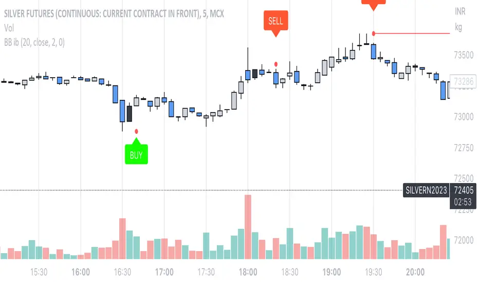
Bollinger Bands Inside barthe indicator name is Bollinger Band inside bar because it uses Bollinger Band and inside bar to take counter-trend positions in the market. whenever this pattern is formed then it can be used to take an entry into the market. the candlestick pattern recognizes 3 candle candlestick. first the mother bar i.e. the medium to the big size candle that intersects with the upper and the lower levels of the Bollinger band. the second candle should be an inside bar i.e. the high and low of the current bar should be less than the previous bar. finally, the last bar who's low should be less than the mother bar in case of the mother bar is at upper levels and if the mother bar is at lower levels then the candle's high should be more than the mother bar. the stop-loss should be high and low of the mother bar respectively. entry should be taken as soon as the low and high of the mother bar is taken out respectively. target should be 1:1 or 20 sma or lower Bollinger band in case the entry is taken from the top. works best if there is a trend and the market takes a pullback and this pattern is formed.
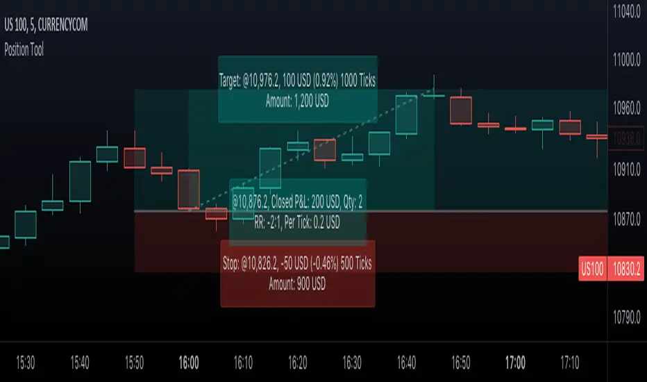
Position Tool█ OVERVIEW
This script is an interactive measurement tool that can be used to evaluate or keep track of trades. Like the long and short position drawing tools, it calculates a risk reward ratio and a risk-adjusted position size from the entry, stop and take profit levels, but it also does much more:
• It can be used to configure long or short trades.
• All monetary values can be expressed in any number of currencies.
• The value of tick/pip movement (which varies with the position's size) is displayed in the currency you have selected.
• The CAGR ( Compound Annual Growth Rate ) for the trade can be displayed.
• It does live tracking of the position.
• You can configure alerts on entries and exits.
█ HOW TO USE IT
Load the indicator on an active chart (see here if you don't know how).
When you first load this script on a chart, you will enter an interactive selection mode where the script asks you to pick three points in price and time on your chart by clicking on the chart. Directions will appear in a blue box at the bottom of the screen with each click of the mouse. The first selection is the entry point for the trade you are considering, which takes into account both the time and level you choose, the next are the take profit and stop levels. Once you have selected all three points, the script will draw trade zones and labels containing the trade metrics. The script determines if the trade is a long or short from the position of the take profit and stop loss levels in relation to the entry price. If the take profit level is above the entry price, the stop must be below and vice versa, otherwise an error occurs.
You can change levels by dragging the handles that appear when you select the indicator, or by entering new values in the script's settings. The only way to re-enter interactive mode is to re-add the indicator to your chart.
Once you place the position tool on a chart, it will appear at the same levels on all symbols you use. If your scale is not set to "Scale price chart only", the position tool's levels will be taken into account when scaling the chart, which can cause the symbol's bars to be compressed. If your scale is set to "Scale price chart only", the position tool will still be there, but it will not impact the scale of the chart's bars, so you won't see it if it sits outside the symbol's price scale.
If you select the position tool on your chart and delete it, this will also delete the indicator from the chart. You will need to re-add it if you want to draw another position tool. You can add multiple instances of the indicator if you need a position tool on more than one of your charts.
█ FEATURES
Display
The position tool displays the following information for entries:
• The entry's price level with an '@' sign before it.
• Open or Closed P&L : For an open trade, the "Open P&L" displays the difference in money value between the entry level and the chart's current price.
For a closed trade, the "Closed P&L" displays the realized P&L on the trade.
• Quantity : The trade size, which takes into account the risk tolerance you set in the script's settings.
• RR : The reward to risk ratio expresses the relationship of the distance between the entry and the take profit level vs the entry and the stop level.
Example: A $100 stop with a $100 target will have a ratio of 1:1, whereas a $200 target with the same stop will have a 2:1 ratio.
• Per tick/pip : Represents the money value of a tick or pip movement.
• CAGR : The Compound Annual Growth Rate will be displayed on the main order label on trades that exceed one day in duration.
This value is calculated the same way as in our CAGR Custom Range indicator.
If the trade duration is less than one day, the metric will not be present in the display.
The stop and take profit levels display:
• Their price level with an '@' sign before it.
• Their distance from the entry in money value, percentage and ticks/pips.
• The projected end money value of the position if the level is reached. These values are calculated based on the trade size and the currency.
Currency adjustments
This indicator modifies the trade label's colors and values based on the final Profit and Loss (P&L), which considers the dynamic exchange rate between base and conversion currencies in its calculations when the conversion currency is a specified value other than the default. Depending on the cross rate between the base and account currencies, this process can yield a negative P&L on an otherwise successful simulated trade.
For instance, if your account is in currency XYZ, you might buy 10 Apple shares at $150 each, with the XYZ to USD exchange rate being 2:1. This purchase would cost you 3000 units of XYZ. Suppose that later on, the shares appreciate to $170 each, and you decide to sell. One might expect this trade to result in profit. However, if the exchange rate has now equalized to 1:1, the return on selling the shares, calculated in XYZ, would only be 1700 units, resulting in a loss of 1300 units XYZ.
The indicator will mark the P&L and the target labels in red in such cases, regardless of whether the market price reached the profit target, as the trade produced a net loss due to reduced funds after currency conversion. Conversely, an otherwise unsuccessful position can result in a net profit in the account currency due to conversion rate fluctuations. The final losses or gains appear in the label metrics, and the corresponding color coding reflects the trade's success or failure.
Settings
The settings in the "Trade sizing" section are used to calculate the position size and the monetary value of trades. Two types of risk can be chosen from the menu; a percentage based risk calculation, or a fixed money value. The risk is used to calculate the quantity of units to purchase to achieve that level of risk exposure. Example: An account size of $1000 and 10% risk will have a projected end amount of $900 if the stop loss is hit. The quantity is a product of this relationship; a projected number of units to allow for the equivalent of $100 of risk exposure over the change in price from the entry to the stop value.
The "Trade levels" allow you to manually set the entry, take profit and stop levels of an existing position tool on your chart.
You can control the appearance of the tool and the values it displays in the settings following these first two sections.
Alerts
Three alerts that will trigger when you configure an alert on this indicator. The first will send an alert when the entry price is breached by price action if that price has not already been breached in the previous price history. This is dependant on the entry location you select when placing the indicator on the chart. The other two alerts will trigger when either the stop loss or the take profit level is breached to signal that a trade exit has occurred.
█ NOTES FOR Pine Script™ CODERS
• Interactive inputs are implemented for input.time() and input.price() . These specialized input functions allow users to interact with a script.
You can create one interactive input for both time and price values by using the same `inline` argument in a pair of input.time() and input.price() function calls.
• We use the `cagr()` function from our ta library.
• The script uses the runtime.error() function to throw an error if the stop and limit prices are not placed on opposing sides of the entry price.
• We use the `currency` parameter in a request.security() call to convert currencies.
Look first. Then leap.
Bitfinex Shorts StratOverview
This strat applies the data from BITFINEX:USDSHORTS to the RSI indicator in order to provide SHORT/LONG entries as the number of contracts goes up and down. Although Bitfinex has lost relevance over the years its generally considered an exchange dominated by smart money rather than retail. I'd like to see if any insights can be gained by following their trading behaviour.
How to use
Select the underlying security you wish to trade and load the indicator. Select the appropriate short security by searching in the Bitfinex Short Symbol. RSI settings apply to short symbol not the actual asset. Strategy shorts the underlying asset when shorts rise and longs when they drop. The shorts symbol will follow the value of the loaded chart. Works best on 4 hour chart.
Why use shorts only rather than both long/shorts?
Bitfinex longs seem to be on a long-term uptrend accounting for 25x the number of shorts. Might be enormous confidence on part of the whales, but more likely reflects selling spot and buying perp. Given the size disparity and price action I don't think longs info is adding much.
Problems with script:
a) We don't really know the intentions of short players (e.g. speculation or hedging spot)
b) The script uses a decline in shorts as a long signal
c) RSI is a blunt tool there are probably better options for calculating high/lows in shorts
d) Shorts are accumulated both at highs and also when BTC price is already heavily trending down. This suggests some are speculative (at the highs) or protective/hedging during a decline
Takeaways:
Based on this strat Bitfinex whales are more wrong than right.
Results don't carry across well into altcoins using the accompanying short symbol. However, what is interesting is that applying the BITFINEX:BTCUSDSHORTS to altcoin charts does work pretty well.
Strat needs some refinement to control for entries under different circumstances.
Probably not a great idea to use this as a strategy in isolation, but highlights how Bitfinex whale behaviour is a good gauge to follow.

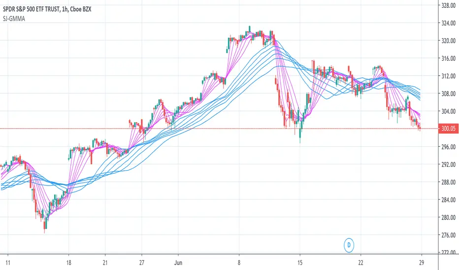
JSun - Guppy Multiple Moving AverAgeThe Guppy Multiple Moving Average (GMMA) is a technical indicator that identifies changing trends, breakouts, and trading opportunities in the price of an asset by combining two groups of moving averages (MA) with different time periods. There is a short-term group of MAs, and a long-term group of MA. Both contain six MAs, for a total of 12. The term gets its name from Daryl Guppy, an Australian trader who is credited with its development.
Key Takeaways:
1. The Gruppy Multiple Moving Average (GMMA) is applied as an overlay on the price chart of an asset.
2. The short-term MAs are typically set at 3, 5, 8, 10, 12, and 15 periods. The longer-term MAs are typically set at 30, 35, 40, 45, 50, and 60.
3. When the short-term group of averages moves above the longer-term group, it indicates a price uptrend in the asset could be emerging.
4. When the short-term group falls below the longer-term group of MAs, a price downtrend in the asset could be starting.
5. When there is lots of separation between the MAs, this helps confirm the price trend in the current direction.
6. If both groups become compressed with each other, or crisscross, it indicates the price has paused and a price trend reversal is possible.
7. Traders often trade in the direction the longer-term MA group is moving, and use the short-term group for trade signals to enter or exit.
Liquidity Sweep & Reversal MapLiquidity Sweep & Reversal Map (LSRM) is a visual tool designed to help traders study how price interacts with key liquidity areas such as daily highs, daily lows, previous-day levels, and potential sweep zones. Its purpose is to map structure, highlight volatility around major reference points, and visualize how price behaves after taking liquidity.
This indicator does not attempt to predict market direction. It simply identifies conditions where price has interacted with a known reference level and marks that interaction for user analysis.
🔍 What This Indicator Shows
1. Key Liquidity Reference Levels
The script automatically draws and updates the following levels:
TH — Today’s High
TL — Today’s Low
PDH — Previous Day High
PDL — Previous Day Low
These levels are widely monitored by many traders and can be helpful when studying liquidity behavior and intraday volatility.
2. Liquidity Sweeps
A liquidity sweep occurs when:
Price briefly moves beyond a major high or low
And then closes back within the prior range
The indicator marks detected sweep interactions with:
BS (Bullish Sweep) when liquidity is taken below a low
SS (Bearish Sweep) when liquidity is taken above a high
A sweep only appears after the bar has closed, helping users analyze completed price structure.
3. Optional Sweep Zones
When enabled, the tool draws a shaded zone between:
The swept wick
The reference level
This can help highlight areas where liquidity was taken.
4. Volume & Candle Filters
The indicator includes optional filters such as:
Relative volume spikes
Strong candle body requirement
These filters are provided only to refine the visual highlight of sweeps; they do not constitute trading signals.
🎛 Customization
Users can configure:
Instrument presets
Sweep buffers
Volume sensitivity
Line visibility and thickness
Label display
Zone visibility
All settings are optional and intended for chart annotation only.
⚠️ Important Notes
This tool is not a trading system, signal generator, or strategy.
It does not provide buy/sell advice or predict future price movement.
All markings are visual aids for chart study and structural analysis only.
Users should rely on their own judgment and independent analysis when making trading decisions.

Volatility-Targeted Momentum Portfolio [BackQuant]Volatility-Targeted Momentum Portfolio
A complete momentum portfolio engine that ranks assets, targets a user-defined volatility, builds long, short, or delta-neutral books, and reports performance with metrics, attribution, Monte Carlo scenarios, allocation pie, and efficiency scatter plots. This description explains the theory and the mechanics so you can configure, validate, and deploy it with intent.
Table of contents
What the script does at a glance
Momentum, what it is, how to know if it is present
Volatility targeting, why and how it is done here
Portfolio construction modes: Long Only, Short Only, Delta Neutral
Regime filter and when the strategy goes to cash
Transaction cost modelling in this script
Backtest metrics and definitions
Performance attribution chart
Monte Carlo simulation
Scatter plot analysis modes
Asset allocation pie chart
Inputs, presets, and deployment checklist
Suggested workflow
1) What the script does at a glance
Pulls a list of up to 15 tickers, computes a simple momentum score on each over a configurable lookback, then volatility-scales their bar-to-bar return stream to a target annualized volatility.
Ranks assets by raw momentum, selects the top 3 and bottom 3, builds positions according to the chosen mode, and gates exposure with a fast regime filter.
Accumulates a portfolio equity curve with risk and performance metrics, optional benchmark buy-and-hold for comparison, and a full alert suite.
Adds visual diagnostics: performance attribution bars, Monte Carlo forward paths, an allocation pie, and scatter plots for risk-return and factor views.
2) Momentum: definition, detection, and validation
Momentum is the tendency of assets that have performed well to continue to perform well, and of underperformers to continue underperforming, over a specific horizon. You operationalize it by selecting a horizon, defining a signal, ranking assets, and trading the leaders versus laggards subject to risk constraints.
Signal choices . Common signals include cumulative return over a lookback window, regression slope on log-price, or normalized rate-of-change. This script uses cumulative return over lookback bars for ranking (variable cr = price/price - 1). It keeps the ranking simple and lets volatility targeting handle risk normalization.
How to know momentum is present .
Leaders and laggards persist across adjacent windows rather than flipping every bar.
Spread between average momentum of leaders and laggards is materially positive in sample.
Cross-sectional dispersion is non-trivial. If everything is flat or highly correlated with no separation, momentum selection will be weak.
Your validation should include a diagnostic that measures whether returns are explained by a momentum regression on the timeseries.
Recommended diagnostic tool . Before running any momentum portfolio, verify that a timeseries exhibits stable directional drift. Use this indicator as a pre-check: It fits a regression to price, exposes slope and goodness-of-fit style context, and helps confirm if there is usable momentum before you force a ranking into a flat regime.
3) Volatility targeting: purpose and implementation here
Purpose . Volatility targeting seeks a more stable risk footprint. High-vol assets get sized down, low-vol assets get sized up, so each contributes more evenly to total risk.
Computation in this script (per asset, rolling):
Return series ret = log(price/price ).
Annualized volatility estimate vol = stdev(ret, lookback) * sqrt(tradingdays).
Leverage multiplier volMult = clamp(targetVol / vol, 0.1, 5.0).
This caps sizing so extremely low-vol assets don’t explode weight and extremely high-vol assets don’t go to zero.
Scaled return stream sr = ret * volMult. This is the per-bar, risk-adjusted building block used in the portfolio combinations.
Interpretation . You are not levering your account on the exchange, you are rescaling the contribution each asset’s daily move has on the modeled equity. In live trading you would reflect this with position sizing or notional exposure.
4) Portfolio construction modes
Cross-sectional ranking . Assets are sorted by cr over the chosen lookback. Top and bottom indices are extracted without ties.
Long Only . Averages the volatility-scaled returns of the top 3 assets: avgRet = mean(sr_top1, sr_top2, sr_top3). Position table shows per-asset leverages and weights proportional to their current volMult.
Short Only . Averages the negative of the volatility-scaled returns of the bottom 3: avgRet = mean(-sr_bot1, -sr_bot2, -sr_bot3). Position table shows short legs.
Delta Neutral . Long the top 3 and short the bottom 3 in equal book sizes. Each side is sized to 50 percent notional internally, with weights within each side proportional to volMult. The return stream mixes the two sides: avgRet = mean(sr_top1,sr_top2,sr_top3, -sr_bot1,-sr_bot2,-sr_bot3).
Notes .
The selection metric is raw momentum, the execution stream is volatility-scaled returns. This separation is deliberate. It avoids letting volatility dominate ranking while still enforcing risk parity at the return contribution stage.
If everything rallies together and dispersion collapses, Long Only may behave like a single beta. Delta Neutral is designed to extract cross-sectional momentum with low net beta.
5) Regime filter
A fast EMA(12) vs EMA(21) filter gates exposure.
Long Only active when EMA12 > EMA21. Otherwise the book is set to cash.
Short Only active when EMA12 < EMA21. Otherwise cash.
Delta Neutral is always active.
This prevents taking long momentum entries during obvious local downtrends and vice versa for shorts. When the filter is false, equity is held flat for that bar.
6) Transaction cost modelling
There are two cost touchpoints in the script.
Per-bar drag . When the regime filter is active, the per-bar return is reduced by fee_rate * avgRet inside netRet = avgRet - (fee_rate * avgRet). This models proportional friction relative to traded impact on that bar.
Turnover-linked fee . The script tracks changes in membership of the top and bottom baskets (top1..top3, bot1..bot3). The intent is to charge fees when composition changes. The template counts changes and scales a fee by change count divided by 6 for the six slots.
Use case: increase fee_rate to reflect taker fees and slippage if you rebalance every bar or trade illiquid assets. Reduce it if you rebalance less often or use maker orders.
Practical advice .
If you rebalance daily, start with 5–20 bps round-trip per switch on liquid futures and adjust per venue.
For crypto perp microcaps, stress higher cost assumptions and add slippage buffers.
If you only rotate on lookback boundaries or at signals, use alert-driven rebalances and lower per-bar drag.
7) Backtest metrics and definitions
The script computes a standard set of portfolio statistics once the start date is reached.
Net Profit percent over the full test.
Max Drawdown percent, tracked from running peaks.
Annualized Mean and Stdev using the chosen trading day count.
Variance is the square of annualized stdev.
Sharpe uses daily mean adjusted by risk-free rate and annualized.
Sortino uses downside stdev only.
Omega ratio of sum of gains to sum of losses.
Gain-to-Pain total gains divided by total losses absolute.
CAGR compounded annual growth from start date to now.
Alpha, Beta versus a user-selected benchmark. Beta from covariance of daily returns, Alpha from CAPM.
Skewness of daily returns.
VaR 95 linear-interpolated 5th percentile of daily returns.
CVaR average of the worst 5 percent of daily returns.
Benchmark Buy-and-Hold equity path for comparison.
8) Performance attribution
Cumulative contribution per asset, adjusted for whether it was held long or short and for its volatility multiplier, aggregated across the backtest. You can filter to winners only or show both sides. The panel is sorted by contribution and includes percent labels.
9) Monte Carlo simulation
The panel draws forward equity paths from either a Normal model parameterized by recent mean and stdev, or non-parametric bootstrap of recent daily returns. You control the sample length, number of simulations, forecast horizon, visibility of individual paths, confidence bands, and a reproducible seed.
Normal uses Box-Muller with your seed. Good for quick, smooth envelopes.
Bootstrap resamples realized returns, preserving fat tails and volatility clustering better than a Gaussian assumption.
Bands show 10th, 25th, 75th, 90th percentiles and the path mean.
10) Scatter plot analysis
Four point-cloud modes, each plotting all assets and a star for the current portfolio position, with quadrant guides and labels.
Risk-Return Efficiency . X is risk proxy from leverage, Y is expected return from annualized momentum. The star shows the current book’s composite.
Momentum vs Volatility . Visualizes whether leaders are also high vol, a cue for turnover and cost expectations.
Beta vs Alpha . X is a beta proxy, Y is risk-adjusted excess return proxy. Useful to see if leaders are just beta.
Leverage vs Momentum . X is volMult, Y is momentum. Shows how volatility targeting is redistributing risk.
11) Asset allocation pie chart
Builds a wheel of current allocations.
Long Only, weights are proportional to each long asset’s current volMult and sum to 100 percent.
Short Only, weights show the short book as positive slices that sum to 100 percent.
Delta Neutral, 50 percent long and 50 percent short books, each side leverage-proportional.
Labels can show asset, percent, and current leverage.
12) Inputs and quick presets
Core
Portfolio Strategy . Long Only, Short Only, Delta Neutral.
Initial Capital . For equity scaling in the panel.
Trading Days/Year . 252 for stocks, 365 for crypto.
Target Volatility . Annualized, drives volMult.
Transaction Fees . Per-bar drag and composition change penalty, see the modelling notes above.
Momentum Lookback . Ranking horizon. Shorter is more reactive, longer is steadier.
Start Date . Ensure every symbol has data back to this date to avoid bias.
Benchmark . Used for alpha, beta, and B&H line.
Diagnostics
Metrics, Equity, B&H, Curve labels, Daily return line, Rolling drawdown fill.
Attribution panel. Toggle winners only to focus on what matters.
Monte Carlo mode with Normal or Bootstrap and confidence bands.
Scatter plot type and styling, labels, and portfolio star.
Pie chart and labels for current allocation.
Presets
Crypto Daily, Long Only . Lookback 25, Target Vol 50 percent, Fees 10 bps, Regime filter on, Metrics and Drawdown on. Monte Carlo Bootstrap with Recent 200 bars for bands.
Crypto Daily, Delta Neutral . Lookback 25, Target Vol 50 percent, Fees 15–25 bps, Regime filter always active for this mode. Use Scatter Risk-Return to monitor efficiency and keep the star near upper left quadrants without drifting rightward.
Equities Daily, Long Only . Lookback 60–120, Target Vol 15–20 percent, Fees 5–10 bps, Regime filter on. Use Benchmark SPX and watch Alpha and Beta to keep the book from becoming index beta.
13) Suggested workflow
Universe sanity check . Pick liquid tickers with stable data. Thin assets distort vol estimates and fees.
Check momentum existence . Run on your timeframe. If slope and fit are weak, widen lookback or avoid that asset or timeframe.
Set risk budget . Choose a target volatility that matches your drawdown tolerance. Higher target increases turnover and cost sensitivity.
Pick mode . Long Only for bull regimes, Short Only for sustained downtrends, Delta Neutral for cross-sectional harvesting when index direction is unclear.
Tune lookback . If leaders rotate too often, lengthen it. If entries lag, shorten it.
Validate cost assumptions . Increase fee_rate and stress Monte Carlo. If the edge vanishes with modest friction, refine selection or lengthen rebalance cadence.
Run attribution . Confirm the strategy’s winners align with intuition and not one unstable outlier.
Use alerts . Enable position change, drawdown, volatility breach, regime, momentum shift, and crash alerts to supervise live runs.
Important implementation details mapped to code
Momentum measure . cr = price / price - 1 per symbol for ranking. Simplicity helps avoid overfitting.
Volatility targeting . vol = stdev(log returns, lookback) * sqrt(tradingdays), volMult = clamp(targetVol / vol, 0.1, 5), sr = ret * volMult.
Selection . Extract indices for top1..top3 and bot1..bot3. The arrays rets, scRets, lev_vals, and ticks_arr track momentum, scaled returns, leverage multipliers, and display tickers respectively.
Regime filter . EMA12 vs EMA21 switch determines if the strategy takes risk for Long or Short modes. Delta Neutral ignores the gate.
Equity update . Equity multiplies by 1 + netRet only when the regime was active in the prior bar. Buy-and-hold benchmark is computed separately for comparison.
Tables . Position tables show current top or bottom assets with leverage and weights. Metric table prints all risk and performance figures.
Visualization panels . Attribution, Monte Carlo, scatter, and pie use the last bars to draw overlays that update as the backtest proceeds.
Final notes
Momentum is a portfolio effect. The edge comes from cross-sectional dispersion, adequate risk normalization, and disciplined turnover control, not from a single best asset call.
Volatility targeting stabilizes path but does not fix selection. Use the momentum regression link above to confirm structure exists before you size into it.
Always test higher lag costs and slippage, then recheck metrics, attribution, and Monte Carlo envelopes. If the edge persists under stress, you have something robust.

3/4-Bar GRG / RGR Pattern (Conditional 4th Candle)This indicator can be used to identify the Green-Red-Green or Red-Green-Red pattern.
It is a price action indicator where a price action which identifies the defeat of buyers and sellers.
If the buyers comprehensively defeat the sellers then the price moves up and if the sellers defeat the buyers then the price moves down.
In my trading experience this is what defines the price movement.
It is a 3 or 4 candle pattern, beyond that i.e, 5 or more candles could mean a very sideways market and unnecessary signal generation.
How does it work?
Upside/Green signal
Say candle 1 is Green, which means buyers stepped in, then candle 2 is Red or a Doji, that means sellers brought the price down. Then if candle 3 is forming to be Green and breaks the closing of the 1st candle and opening of the 2nd candle, then a green arrow will appear and that is the place where you want to take your trade.
Here the buyers defeated the sellers.
Sometimes candle 3 falls short but candle 4 breaks candle 1's closing and candle 2's opening price. We can enter on candle 4.
Important - We need to enter the trade as soon as the price moves above the candle 1 and 2's body and should not wait for the 3rd or 4th candle to close. Ignore wicks.
I have restricted it to 4 candles and that is all that is needed. More than that is a longer sideways market.
I call it the +-+ or GRG pattern.
Stop loss can be candle 2's mid for safe traders (that includes me) or candle 2's body low for risky traders.
Back testing suggests that body low will be useless and result in more points in loss because for the bigger move this point will not be touched, so why not get out faster.
Downside/Red signal
Say candle 1 is Red, which means sellers stepped in, then candle 2 is Green or a Doji, that means buyers took the price up. Then if candle 3 is forming to be Red and breaks the closing of the 1st candle and opening of the 2nd candle then a Red arrow will appear and that is the place where you want to take your trade.
Sometimes candle 3 falls short but candle 4 breaks candle 1's closing and candle 2's opening price. We can enter on candle 4.
We need to enter the trade as soon as the price moves below the candle 1 and 2's body and should not wait for the 3rd or 4th candle to close.
I have restricted it to 4 candles and that is all that is needed. More than that is a longer sideways market.
I call it the -+- or RGR pattern.
Stop loss can be candle 2's mid for safe traders ( that includes me) or candle 2's body high for risky traders.
Back testing suggests that body high will be useless and result in more points in loss because for the bigger move this point will not be touched, so why not get out faster.
Important Settings
You can enable or disable the 4th candle signal to avoid the noise, but at times I have noticed that the 4th candle gives a very strong signal or I can say that the strong signal falls on the 4th candle. This is mostly a coincidence.
You can also configure how many previous bars should the signal be generated for. 10 to 30 is good enough. To backtest increase it to 2000 or 5000 for example.
Rest are self explanatory.
Pointers
If after taking the trade, the next candle moves in your direction and closes strong bullish or bearish, then move SL to break even and after that you can trail it.
If a upside trade hits SL and immediately a down side trade signal is generated on the next candle then take it. Vice versa is true.
Trades need to be taken on previous 2 candle's body high or low combined and not the wicks.
The most losses a trader takes is on a sideways day and because in our strategy the stop loss is so small that even on a sideways day we'll get out with a little profit or worst break even.
Hold targets for longer targets and don't panic.
If last 3-4 days have been sideways then there is a good probability that day will be trending so we can hold our trade for longer targets. Target to hold the trade for whole day and not exit till the day closes.
In general avoid trading in the middle of the day for index and stocks. Divide the day into 3 parts and avoid the middle.
Use Support/Resistance, 10, 20, 50, 200 EMA/SMA, Gaps, Whole/Round numbers(very imp) for identifying targets.
Trail your SL.
For indexes I would use 5 min and 15 min timeframe.
For commodities and crypto we can use higher timeframe as well. Look for signals during volatile time durations and avoid trading the whole day. Signal usually gives good targets on those times.
If a GRG or RGR pattern appears on a daily timeframe then this is our time to go big.
Minimum Risk to Reward should be 1:2 and for longer targets can be 1:4 to 1:10.
Trade with small lot size. Money management will happen automatically.
With small lot size and correct Risk-Re ward we can be very profitable. Don't trade with big lot size.
Stay in the market for longer and collect points not money.
Very imp - Watch market and learn to generate a market view.
Very imp - Only 4 candles are needed in trading - strong bullish, strong bearish, hammer, inverse hammer and doji.
Go big on bearish days for option traders. Puts are better bought and Calls are better sold.
Cluster of green signals can lead to bigger move on the upside and vice versa for red signals.
Most of this is what I learned from successful traders (from the top 2%) only the indicator is mine.
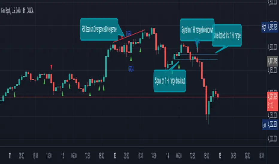
Wolf Exit Oscillator Enhanced
# Wolf Exit Oscillator Enhanced
## What it is (quick take)
**Wolf Exit Oscillator Enhanced** is a clean, rules-first **exit timing tool** built on the **True Strength Index (TSI)** with two optional safeguards:
1. **Signal-line crossover** (to avoid bailing on shallow dips), and
2. **EMA confirmation** (price-based “is the trend actually weakening/strengthening?” check).
Use it to standardize when you **take profits, cut losers, or scale out**—especially after momentum runs hot or cold.
> Works best **paired** with:
>
> * **ABS NR — Fail-Safe Confirm (v4.2.2)** for entries
> * **ABS Companion Oscillator — Trend / Exhaustion / New Trend** for trend/exhaustion context
---
## How to use it (operational workflow)
1. **Set your bands**
* `exitHigh` and `exitLow` mark “overcooked” zones on the TSI scale (default: +60 / –60).
* Above `exitHigh` = momentum stretched **up** (good place to **exit shorts** or **take long profits**).
* Below `exitLow` = momentum stretched **down** (good place to **exit longs** or **take short profits**).
2. **Choose strictness**
* **Base mode**: the moment TSI crosses out of a band, you get an exit signal.
* **Add Signal-Line Cross** (`enableSignalX = true`): require TSI to cross its signal in the same direction → **fewer, cleaner exits**.
* **Add EMA Filter** (`enableEMAFilter = true`): also require **price** to confirm (e.g., long exit only if price < EMA). This avoids bailing during healthy trends.
3. **Execute with structure**
* **Full exit** when a signal fires, or
* **Scale out** (e.g., 50% on first signal, remainder on trail/secondary signal), or
* **Move stop** to lock gains once an exit signal prints.
4. **Alerts**
* Set to **“Once per bar close”** to avoid intrabar flip-flop.
* Use the two provided alert names for automation (see “Alerts” below).
---
## Signals & visuals
* **TSI line** (solid) and **Signal line** (dashed) with optional **histogram** (TSI − Signal).
* **Horizontal bands** at `exitHigh` and `exitLow`.
* **Labels**:
* **Exit Long** appears when long-side momentum breaks down (below `exitLow`, plus any enabled filters).
* **Exit Short** appears when short-side momentum breaks down (above `exitHigh`, plus any enabled filters).
**Alerts (stable names):**
* **WolfExit — Exit Long**
* **WolfExit — Exit Short**
---
## Non-repainting behavior (what to expect)
* The oscillator is computed with **EMAs on current timeframe**—no higher-timeframe lookahead, no repaint.
* **Intrabar**: TSI/Signal can fluctuate; use **bar-close evaluation** (and alert setting “Once per bar close”) to lock signals.
* If you enable the EMA filter, that check is also evaluated at bar close.
---
## Every input explained (and how changing it alters behavior)
### Momentum engine (TSI)
* **TSI Long EMA Length (`tsiLongLen`, default 25)**
Higher = smoother, slower momentum; fewer signals. Lower = twitchier, more signals.
* **TSI Short EMA Length (`tsiShortLen`, default 13)**
Fine-tunes responsiveness on top of the long length. Lower short → snappier TSI.
* **TSI Signal Line Length (`tsisigLen`, default 7)**
Higher = slower signal line (harder to cross) → fewer signals. Lower = easier crosses → more signals.
### Thresholds (the bands)
* **Exit Threshold High (`exitHigh`, default +60)**
Raise to demand **stronger** overbought before signaling short exits / long profit-takes. Lower to trigger sooner.
* **Exit Threshold Low (`exitLow`, default −60)**
Raise (toward 0) to trigger **earlier** on longs; lower (more negative) to wait for deeper downside stretch.
### Confirmation layers
* **Require Signal Line Crossover (`enableSignalX`, default true)**
On = TSI must cross its signal (same direction as exit) → **filters out shallow wiggles**. Off = faster, more frequent exits.
* **Enable EMA Confirmation Filter (`enableEMAFilter`, default true)**
On = require **price < EMA** for **Exit Long** and **price > EMA** for **Exit Short**.
* **EMA Exit Confirmation Length (`exitEMALen`, default 50)**
Higher = **trendier** filter (harder to flip) → fewer exits; Lower = more reactive → more exits.
### Visuals
* **Show Histogram (`showHist`)**
On = quick visual for TSI–Signal spread (helps spot weakening momentum before a cross).
* **Plot Exit Signals (`showSignals`)**
Toggle labels if you only want the lines/bands with alerts.
---
## Tuning recipes (quick, practical)
* **Strong trend days (avoid premature exits)**
* Keep **`enableSignalX = true`** and **`enableEMAFilter = true`**
* Increase **`exitEMALen`** (e.g., 80)
* Consider raising **`exitHigh`** to 65–70 (and lowering **`exitLow`** to −65/−70)
* **Choppy/range days (exit faster, take the cash)**
* **`enableEMAFilter = false`** (don’t wait for price filter)
* **`enableSignalX`** optional; try off for quicker responses
* Bring bands closer to **±50** to take profits earlier
* **Scalping / lower timeframes**
* Shorten **TSI lengths** a bit (e.g., 21/9/5)
* Consider **`exitHigh=55 / exitLow=-55`**
* Keep **histogram on** to visualize momentum flip risk
* **Swing trading / higher timeframes**
* Lengthen **TSI** (e.g., 35/21/9) and **`exitEMALen`** (e.g., 100)
* Wider bands (±65 to ±75) to catch bigger moves before exiting
---
## Playbooks (how to actually trade it)
* **Entry from ABS NR FS, exit with Wolf**
* Take entries from **ABS NR — Fail-Safe Confirm** (triangle).
* Use **Wolf Exit** to scale out: 50% on first exit label, trail remainder with price/EMA or your stop logic.
* **Pyramid & protect**
* Add on re-accelerations (TSI pulls back toward zero without breaching the opposite band).
* The first **Exit** signal → take partial, raise stop to last higher low / lower high.
* **Mean-reversion fade management**
* When fading with ABS NR (KC band pokes + stretched |Z|), target the first opposite **Exit** signal as your “don’t overstay” cue.
---
## Suggested starting points
* **Day trading (5–15m):**
* TSI: **25 / 13 / 7** (default)
* Bands: **+60 / −60**
* Confirmations: **SignalX = on**, **EMA Filter = on**, **EMA Len = 50**
* Alerts: **Once per bar close**
* **Scalping (1–3m):**
* TSI: **21 / 9 / 5**
* Bands: **±55**
* Confirmations: **SignalX = on**, **EMA Filter = off** (optional for speed)
* **Swing (1h–D):**
* TSI: **35 / 21 / 9**
* Bands: **+65 / −65** (or ±70)
* Confirmations: **SignalX = on**, **EMA Filter = on**, **EMA Len = 100**
---
## Best-practice pairings
* **Entries:** **ABS NR — Fail-Safe Confirm (v4.2.2)**
* Take ABS triangles; let Wolf standardize exits so you’re not guessing.
* **Context:** **ABS Companion Oscillator**
* Prefer holding longer when the companion stays above (for longs) or below (for shorts) its neutral band and **no EXH tag** prints.
* If companion flags **EXH** against your position, tighten stops; Wolf’s next exit signal becomes high priority.
---
## Notes & disclaimers
* This is an **exit signal tool**, not a strategy or broker.
* Signals are strongest when aligned with your **entry logic** and a **risk framework** (position sizing, stops, partials).
* All evaluations are **current timeframe**; no higher-timeframe lookahead is used.
* Markets change—tune the bands and confirmations per symbol/timeframe.
---
**Tip:** Keep your alerts simple—one for **Exit Long**, one for **Exit Short**, **Once per bar close**. Use partial exits on the first signal, and let your stop/trailing logic handle the rest.

Gold Breakout Strategy - RR 4Strategy Name: Gold Breakout Strategy - RR 4
🧠 Main Objective
This strategy aims to capitalize on breakouts from the Donchian Channel on Gold (XAU/USD) by filtering trades with:
Volume confirmation,
A custom momentum indicator (LWTI - Linear Weighted Trend Index),
And a specific trading session (8 PM to 8 AM Quebec time — GMT-5).
It takes only one trade per day, either a buy or a sell, using a fixed stop-loss at the wick of the breakout candle and a 4:1 reward-to-risk (RR) ratio.
📊 Indicators Used
Donchian Channel
Length: 96
Detects breakouts of recent highs or lows.
Volume
Simple Moving Average (SMA) over 30 bars.
A breakout is only valid if the current volume is above the SMA.
LWTI (Linear Weighted Trend Index)
Measures momentum using price differences over 25 bars, smoothed over 5.
Used to confirm trend direction:
Buy when LWTI > its smoothed version (uptrend).
Sell when LWTI < its smoothed version (downtrend).
⏰ Time Filter
The strategy only allows entries between 8 PM and 8 AM (GMT-5 / Quebec time).
A timestamp-based filter ensures the system recognizes the correct trading session even across midnight.
📌 Entry Conditions
🟢 Buy (Long)
Price breaks above the previous Donchian Channel high.
The current channel high is higher than the previous one.
Volume is above its moving average.
LWTI confirms an uptrend.
The time is within the trading session (20:00 to 08:00).
No trade has been taken yet today.
🔴 Sell (Short)
Price breaks below the previous Donchian Channel low.
The current channel low is lower than the previous one.
Volume is above its moving average.
LWTI confirms a downtrend.
The time is within the trading session.
No trade has been taken yet today.
💸 Trade Management
Stop-Loss (SL):
For long entries: placed below the wick low of the breakout candle.
For short entries: placed above the wick high of the breakout candle.
Take-Profit (TP):
Set at a fixed 4:1 reward-to-risk ratio.
Calculated as 4x the distance between the entry price and stop-loss.
No trailing stop, no break-even, no scaling in/out.
🎨 Visuals
Green triangle appears below the candle on a buy signal.
Red triangle appears above the candle on a sell signal.
Donchian Channel lines are plotted on the chart.
The strategy is designed for the 5-minute timeframe.
🔄 One Trade Per Day Rule
Once a trade is taken (buy or sell), no more trades will be executed for the rest of the day. This prevents overtrading and limits exposure.

Enigma Sniper 369The "Enigma Sniper 369" is a custom-built Pine Script indicator designed for TradingView, tailored specifically for forex traders seeking high-probability entries during high-volatility market sessions.
Unlike generic trend-following or scalping tools, this indicator uniquely combines session-based "kill zones" (London and US sessions), momentum-based candle analysis, and an optional EMA trend filter to pinpoint liquidity grabs and reversal opportunities.
Its originality lies in its focus on liquidity hunting—identifying levels where stop losses are likely clustered (around swing highs/lows and wick midpoints)—and providing visual entry zones that are dynamically removed once price breaches them, reducing clutter and focusing on actionable signals.
The name "369" reflects the structured approach of three key components (session timing, candle logic, and trend filter) working in harmony to snipe precise entries.
What It Does
"Enigma Sniper 369" identifies potential buy and sell opportunities by drawing two types of horizontal lines on the chart during user-defined London and US
session kill zones:
Solid Lines: Mark the swing low (for buys) or swing high (for sells) of a trigger candle, indicating a potential entry point where stop losses might be clustered.
Dotted Lines: Mark the 50% level of the candle’s wick (lower wick for buys, upper wick for sells), serving as a secondary confirmation zone for entries or tighter stop-loss placement.
These lines are plotted only when specific candle conditions are met within the kill zones, and they are automatically deleted once the price crosses them, signaling that the liquidity at that level has likely been grabbed. The indicator also includes an optional EMA filter to ensure trades align with the broader trend, reducing false signals in choppy markets.
How It Works
The indicator’s logic is built on a multi-layered approach:
Kill Zone Timing: Trades are only considered during user-defined London and US session hours (e.g., London from 02:00 to 12:00 UTC, as seen in the screenshots). These sessions are known for high volatility and liquidity, making them ideal for capturing institutional moves.
Candle-Based Momentum Logic:
Buy Signal: A candle must close above its midpoint (indicating bullish momentum) and have a lower low than the previous candle (suggesting a potential liquidity grab below the previous swing low). This is expressed as close > (high + low) / 2 and low < low .
Sell Signal: A candle must close below its midpoint (bearish momentum) and have a higher high than the previous candle (indicating a potential liquidity grab above the previous swing high), expressed as close < (high + low) / 2 and high > high .
These conditions ensure the indicator targets candles that break recent structure to hunt stop losses while showing directional momentum.
Optional EMA Filter: A 50-period EMA (customizable) can be enabled to filter signals based on trend direction.
Buy signals are only generated if the EMA is trending upward (ema_value > ema_value ), and sell signals require a downward EMA trend (ema_value < ema_value ). This reduces noise by aligning entries with the broader market trend.
Liquidity Levels and Deletion Logic:
For a buy signal, a solid green line is drawn at the candle’s low, and a dotted green line at the 50% level of the lower wick (from the candle body’s bottom to the low).
For a sell signal, a solid red line is drawn at the candle’s high, and a dotted red line at the 50% level of the upper wick (from the body’s top to the high).
These lines extend to the right until the price crosses them, at which point they are deleted, indicating the liquidity at that level has been taken (e.g., stop losses triggered).
Alerts: The indicator includes alert conditions for buy and sell signals, notifying traders when a new setup is identified.
Underlying Concepts
The indicator is grounded in the concept of liquidity hunting, a strategy often employed by institutional traders. Markets frequently move to levels where stop losses are clustered—typically just beyond swing highs or lows—before reversing in the opposite direction. The "Enigma Sniper 369" targets these moves by identifying candles that break structure (e.g., a lower low or higher high) during high-volatility sessions, suggesting a potential sweep of stop losses. The 50% wick level acts as a secondary confirmation, as this midpoint often represents a zone where tighter stop losses are placed by retail traders. The optional EMA filter adds a trend-following element, ensuring entries are taken in the direction of the broader market momentum, which is particularly useful on lower timeframes like the 15-minute chart shown in the screenshots.
How to Use It
Here’s a step-by-step guide based on the provided usage example on the GBP/USD 15-minute chart:
Setup the Indicator: Add "Enigma Sniper 369" to your TradingView chart. Adjust the London and US session hours to match your timezone (e.g., London from 02:00 to 12:00 UTC, US from 13:00 to 22:00 UTC). Customize the EMA period (default 50) and line styles/colors if desired.
Identify Kill Zones: The indicator highlights the London session in light green and the US session in light purple, as seen in the screenshots. Focus on these periods for signals, as they are the most volatile and likely to produce liquidity grabs.
Wait for a Signal: Look for solid and dotted lines to appear during the kill zones:
Buy Setup: A solid green line at the swing low and a dotted green line at the 50% lower wick level indicate a potential buy. This suggests the market may have grabbed liquidity below the swing low and is now poised to move higher.
Sell Setup: A solid red line at the swing high and a dotted red line at the 50% upper wick level indicate a potential sell, suggesting liquidity was taken above the swing high.
Place Your Trade:
For a buy, set a buy limit order at the dotted green line (50% wick level), as this is a more conservative entry point. Place your stop loss just below the solid green line (swing low) to cover the full swing. For example, in the screenshots, the market retraces to the dotted line at 1.32980 after a liquidity grab below the swing low, triggering a buy limit order.
For a sell, set a sell limit order at the dotted red line, with a stop loss just above the solid red line.
Monitor Price Action: Once the price crosses a line, it is deleted, indicating the liquidity at that level has been taken. In the screenshots, after the buy limit is triggered, the market moves higher, confirming the setup. The caption notes, “The market returns and tags us in long with a buy limit,” highlighting this retracement strategy.
Additional Context: Use the indicator to identify liquidity levels that may be targeted later. For example, the screenshot notes, “If a new session is about to open I will wait for the grab liquidity to go long,” showing how the indicator can be used to anticipate future moves at session opens (e.g., London open at 1.32980).
Risk Management: Always set a stop loss below the swing low (for buys) or above the swing high (for sells) to protect against adverse moves. The 50% wick level helps tighten entries, improving the risk-reward ratio.
Practical Example
On the GBP/USD 15-minute chart, during the London session (02:00 UTC), the indicator identifies a buy setup with a solid green line at 1.32901 (swing low) and a dotted green line at 1.32980 (50% wick level). The market initially dips below the swing low, grabbing liquidity, then retraces to the dotted line, triggering a buy limit order. The price subsequently rises to 1.33404, yielding a profitable trade. The user notes, “The logic is in the last candle it provides new level to go long,” emphasizing the indicator’s ability to identify fresh levels after a liquidity sweep.
Customization Tips
Adjust the EMA period to suit your timeframe (e.g., a shorter period like 20 for faster signals on lower timeframes).
Modify the session hours to align with your broker’s timezone or specific market conditions.
Use the alert feature to get notified of new setups without constantly monitoring the chart.
Why It’s Useful for Traders
The "Enigma Sniper 369" stands out by combining session timing, momentum-based candle analysis, and liquidity hunting into a single tool. It provides clear, actionable levels for entries and stop losses, removes invalid signals dynamically, and aligns trades with high-probability market conditions. Whether you’re a scalper looking for quick moves during London open or a swing trader targeting session-based reversals, this indicator offers a structured, data-driven approach to trading.
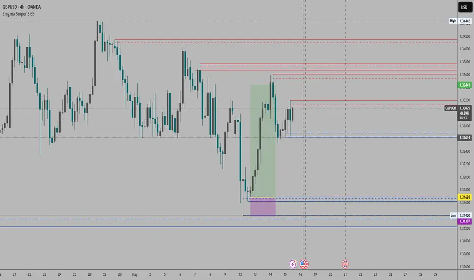
EXODUS EXODUS by (DAFE) Trading Systems
EXODUS is a sophisticated trading algorithm built by Dskyz (DAFE) Trading Systems for competitive and competition purposes, designed to identify high-probability trades with robust risk management. this strategy leverages a multi-signal voting system, combining three core components—SPR, VWMO, and VEI—alongside ADX, choppiness filters, and ATR-based volatility gates to ensure trades are taken only in favorable market conditions. the algo uses a take-profit to stop-loss ratio, dynamic position sizing, and a strict voting mechanism requiring all signals to align before entering a trade.
EXODUS was not overfitted for any specific symbol. instead, it uses a generic tuned setting, making it versatile across various markets. while it can trade futures, it’s not currently set up for it but has the potential to do more with further development. visuals are intentionally minimal due to its competition focus, prioritizing performance over aesthetics. a more visually stunning version may be released in the future with enhanced graphics.
The Unique Core Components Developed for EXODUS
SPR (Session Price Recalibration)
SPR measures momentum during regular trading hours (RTH, 0930-1600, America/New_York) to catch session-specific trends.
spr_lookback = input.int(15, "SPR Lookback") this sets how many bars back SPR looks to calculate momentum (default 15 bars). it compares the current session’s price-volume score to the score 15 bars ago to gauge momentum strength.
how it works: a longer lookback smooths out the signal, focusing on bigger trends. a shorter one makes SPR more sensitive to recent moves.
how to adjust: on a 1-hour chart, 15 bars is 15 hours (about 2 trading days). if you’re on a shorter timeframe like 5 minutes, 15 bars is just 75 minutes, so you might want to increase it to 50 or 100 to capture more meaningful trends. if you’re trading a choppy stock, a shorter lookback (like 5) can help catch quick moves, but it might give more false signals.
spr_threshold = input.float (0.7, "SPR Threshold")
this is the cutoff for SPR to vote for a trade (default 0.7). if SPR’s normalized value is above 0.7, it votes for a long; below -0.7, it votes for a short.
how it works: SPR normalizes its momentum score by ATR, so this threshold ensures only strong moves count. a higher threshold means fewer trades but higher conviction.
how to adjust: if you’re getting too few trades, lower it to 0.5 to let more signals through. if you’re seeing too many false entries, raise it to 1.0 for stricter filtering. test on your chart to find a balance.
spr_atr_length = input.int(21, "SPR ATR Length") this sets the ATR period (default 21 bars) used to normalize SPR’s momentum score. ATR measures volatility, so this makes SPR’s signal relative to market conditions.
how it works: a longer ATR period (like 21) smooths out volatility, making SPR less jumpy. a shorter one makes it more reactive.
how to adjust: if you’re trading a volatile stock like TSLA, a longer period (30 or 50) can help avoid noise. for a calmer stock, try 10 to make SPR more responsive. match this to your timeframe—shorter timeframes might need a shorter ATR.
rth_session = input.session("0930-1600","SPR: RTH Sess.") rth_timezone = "America/New_York" this defines the session SPR uses (0930-1600, New York time). SPR only calculates momentum during these hours to focus on RTH activity.
how it works: it ignores pre-market or after-hours noise, ensuring SPR captures the main market action.
how to adjust: if you trade a different session (like London hours, 0300-1200 EST), change the session to match. you can also adjust the timezone if you’re in a different region, like "Europe/London". just make sure your chart’s timezone aligns with this setting.
VWMO (Volume-Weighted Momentum Oscillator)
VWMO measures momentum weighted by volume to spot sustained, high-conviction moves.
vwmo_momlen = input.int(21, "VWMO Momentum Length") this sets how many bars back VWMO looks to calculate price momentum (default 21 bars). it takes the price change (close minus close 21 bars ago).
how it works: a longer period captures bigger trends, while a shorter one reacts to recent swings.
how to adjust: on a daily chart, 21 bars is about a month—good for trend trading. on a 5-minute chart, it’s just 105 minutes, so you might bump it to 50 or 100 for more meaningful moves. if you want faster signals, drop it to 10, but expect more noise.
vwmo_volback = input.int(30, "VWMO Volume Lookback") this sets the period for calculating average volume (default 30 bars). VWMO weights momentum by volume divided by this average.
how it works: it compares current volume to the average to see if a move has strong participation. a longer lookback smooths the average, while a shorter one makes it more sensitive.
how to adjust: for stocks with spiky volume (like NVDA on earnings), a longer lookback (50 or 100) avoids overreacting to one-off spikes. for steady volume stocks, try 20. match this to your timeframe—shorter timeframes might need a shorter lookback.
vwmo_smooth = input.int(9, "VWMO Smoothing")
this sets the SMA period to smooth VWMO’s raw momentum (default 9 bars).
how it works: smoothing reduces noise in the signal, making VWMO more reliable for voting. a longer smoothing period cuts more noise but adds lag.
how to adjust: if VWMO is too jumpy (lots of false votes), increase to 15. if it’s too slow and missing trades, drop to 5. test on your chart to see what keeps the signal clean but responsive.
vwmo_threshold = input.float(10, "VWMO Threshold") this is the cutoff for VWMO to vote for a trade (default 10). above 10, it votes for a long; below -10, a short.
how it works: it ensures only strong momentum signals count. a higher threshold means fewer but stronger trades.
how to adjust: if you want more trades, lower it to 5. if you’re getting too many weak signals, raise it to 15. this depends on your market—volatile stocks might need a higher threshold to filter noise.
VEI (Velocity Efficiency Index)
VEI measures market efficiency and velocity to filter out choppy moves and focus on strong trends.
vei_eflen = input.int(14, "VEI Efficiency Smoothing") this sets the EMA period for smoothing VEI’s efficiency calc (bar range / volume, default 14 bars).
how it works: efficiency is how much price moves per unit of volume. smoothing it with an EMA reduces noise, focusing on consistent efficiency. a longer period smooths more but adds lag.
how to adjust: for choppy markets, increase to 20 to filter out noise. for faster markets, drop to 10 for quicker signals. this should match your timeframe—shorter timeframes might need a shorter period.
vei_momlen = input.int(8, "VEI Momentum Length") this sets how many bars back VEI looks to calculate momentum in efficiency (default 8 bars).
how it works: it measures the change in smoothed efficiency over 8 bars, then adjusts for inertia (volume-to-range). a longer period captures bigger shifts, while a shorter one reacts faster.
how to adjust: if VEI is missing quick reversals, drop to 5. if it’s too noisy, raise to 12. test on your chart to see what catches the right moves without too many false signals.
vei_threshold = input.float(4.5, "VEI Threshold") this is the cutoff for VEI to vote for a trade (default 4.5). above 4.5, it votes for a long; below -4.5, a short.
how it works: it ensures only strong, efficient moves count. a higher threshold means fewer trades but higher quality.
how to adjust: if you’re not getting enough trades, lower to 3. if you’re seeing too many false entries, raise to 6. this depends on your market—fast stocks like NQ1 might need a lower threshold.
Features
Multi-Signal Voting: requires all three signals (SPR, VWMO, VEI) to align for a trade, ensuring high-probability setups.
Risk Management: uses ATR-based stops (2.1x) and take-profits (4.1x), with dynamic position sizing based on a risk percentage (default 0.4%).
Market Filters: ADX (default 27) ensures trending conditions, choppiness index (default 54.5) avoids sideways markets, and ATR expansion (default 1.12) confirms volatility.
Dashboard: provides real-time stats like SPR, VWMO, VEI values, net P/L, win rate, and streak, with a clean, functional design.
Visuals
EXODUS prioritizes performance over visuals, as it was built for competitive and competition purposes. entry/exit signals are marked with simple labels and shapes, and a basic heatmap highlights market regimes. a more visually stunning update may be released later, with enhanced graphics and overlays.
Usage
EXODUS is designed for stocks and ETFs but can be adapted for futures with adjustments. it performs best in trending markets with sufficient volatility, as confirmed by its generic tuning across symbols like TSLA, AMD, NVDA, and NQ1. adjust inputs like SPR threshold, VWMO smoothing, or VEI momentum length to suit specific assets or timeframes.
Setting I used: (Again, these are a generic setting, each security needs to be fine tuned)
SPR LB = 19 SPR TH = 0.5 SPR ATR L= 21 SPR RTH Sess: 9:30 – 16:00
VWMO L = 21 VWMO LB = 18 VWMO S = 6 VWMO T = 8
VEI ES = 14 VEI ML = 21 VEI T = 4
R % = 0.4
ATR L = 21 ATR M (S) =1.1 TP Multi = 2.1 ATR min mult = 0.8 ATR Expansion = 1.02
ADX L = 21 Min ADX = 25
Choppiness Index = 14 Chop. Max T = 55.5
Backtesting: TSLA
Frame: Jan 02, 2018, 08:00 — May 01, 2025, 09:00
Slippage: 3
Commission .01
Disclaimer
this strategy is for educational purposes. past performance is not indicative of future results. trading involves significant risk, and you should only trade with capital you can afford to lose. always backtest and validate any strategy before using it in live markets.
(This publishing will most likely be taken down do to some miscellaneous rule about properly displaying charting symbols, or whatever. Once I've identified what part of the publishing they want to pick on, I'll adjust and repost.)
About the Author
Dskyz (DAFE) Trading Systems is dedicated to building high-performance trading algorithms. EXODUS is a product of rigorous research and development, aimed at delivering consistent, and data-driven trading solutions.
Use it with discipline. Use it with clarity. Trade smarter.
**I will continue to release incredible strategies and indicators until I turn this into a brand or until someone offers me a contract.
2025 Created by Dskyz, powered by DAFE Trading Systems. Trade smart, trade bold.

Dskyz (DAFE) Quantum Sentiment Flux - Beginners Dskyz (DAFE) Quantum Sentiment Flux - Beginners:
Welcome to the Dskyz (DAFE) Quantum Sentiment Flux - Beginners , a strategy and concept that’s your ultimate wingman for trading futures like MNQ, NQ, MES, and ES. This gem combines lightning-fast momentum signals, market sentiment smarts, and bulletproof risk management into a system so intuitive, even newbies can trade like pros. With clean DAFE visuals, preset modes for every vibe, and a revamped dashboard that’s basically a market GPS, this strategy makes futures trading feel like a high-octane sci-fi mission.
Built on the Dskyz (DAFE) legacy of Aurora Divergence, the Quantum Sentiment Flux is designed to empower beginners while giving seasoned traders a lean, sentiment-driven edge. It uses fast/slow EMA crossovers for entries, filters trades with VIX, SPX trends, and sector breadth, and keeps your account safe with adaptive stops and cooldowns. Tuned for more action with faster signals and a slick bottom-left dashboard, this updated version is ready to light up your charts and outsmart institutional traps. Let’s dive into why this strat’s a must-have and break down its brilliance.
Why Traders Need This Strategy
Futures markets are a wild ride—fast moves, volatility spikes (like the April 28, 2025 NQ 1k-point drop), and institutional games that can wreck unprepared traders. Beginners often get lost in complex systems or burned by impulsive trades. The Quantum Sentiment Flux is the antidote, offering:
Dead-Simple Setup: Preset modes (Aggressive, Balanced, Conservative) auto-tune signals, risk, and sizing, so you can trade without a quant degree.
Sentiment Superpower: VIX filter, SPX trend, and sector breadth visuals keep you aligned with market health, dodging chop and riding trends.
Ironclad Safety: Tighter ATR-based stops, 2:1 take-profits, and preset cooldowns protect your capital, even in chaotic sessions.
Next-Level Visuals: Green/red entry triangles, vibrant EMAs, a sector breadth background, and a beefed-up dashboard make signals and context pop.
DAFE Swagger: The clean aesthetics, sleek dashboard—ties it to Dskyz’s elite brand, making your charts a work of art.
Traders need this because it’s a plug-and-play system that blends beginner-friendly simplicity with pro-level market awareness. Whether you’re just starting or scalping 5min MNQ, this strat’s your key to trading with confidence and style.
Strategy Components
1. Core Signal Logic (High-Speed Momentum)
The strategy’s engine is a momentum-based system using fast and slow Exponential Moving Averages (EMAs), now tuned for faster, more frequent trades.
How It Works:
Fast/Slow EMAs: Fast EMA (Aggressive: 5, Balanced: 7, Conservative: 9 bars) and slow EMA (12/14/18 bars) track short-term vs. longer-term momentum.
Crossover Signals:
Buy: Fast EMA crosses above slow EMA, and trend_dir = 1 (fast EMA > slow EMA + ATR * strength threshold).
Sell: Fast EMA crosses below slow EMA, and trend_dir = -1 (fast EMA < slow EMA - ATR * strength threshold).
Strength Filter: ma_strength = fast EMA - slow EMA must exceed an ATR-scaled threshold (Aggressive: 0.15, Balanced: 0.18, Conservative: 0.25) for robust signals.
Trend Direction: trend_dir confirms momentum, filtering out weak crossovers in choppy markets.
Evolution:
Faster EMAs (down from 7–10/21–50) catch short-term trends, perfect for active futures markets.
Lower strength thresholds (0.15–0.25 vs. 0.3–0.5) make signals more sensitive, boosting trade frequency without sacrificing quality.
Preset tuning ensures beginners get optimized settings, while pros can tweak via mode selection.
2. Market Sentiment Filters
The strategy leans hard into market sentiment with a VIX filter, SPX trend analysis, and sector breadth visuals, keeping trades aligned with the big picture.
VIX Filter:
Logic: Blocks long entries if VIX > threshold (default: 20, can_long = vix_close < vix_limit). Shorts are always allowed (can_short = true).
Impact: Prevents longs during high-fear markets (e.g., VIX spikes in crashes), while allowing shorts to capitalize on downturns.
SPX Trend Filter:
Logic: Compares S&P 500 (SPX) close to its SMA (Aggressive: 5, Balanced: 8, Conservative: 12 bars). spx_trend = 1 (UP) if close > SMA, -1 (DOWN) if < SMA, 0 (FLAT) if neutral.
Impact: Provides dashboard context, encouraging trades that align with market direction (e.g., longs in UP trend).
Sector Breadth (Visual):
Logic: Tracks 10 sector ETFs (XLK, XLF, XLE, etc.) vs. their SMAs (same lengths as SPX). Each sector scores +1 (bullish), -1 (bearish), or 0 (neutral), summed as breadth (-10 to +10).
Display: Green background if breadth > 4, red if breadth < -4, else neutral. Dashboard shows sector trends (↑/↓/-).
Impact: Faster SMA lengths make breadth more responsive, reflecting sector rotations (e.g., tech surging, energy lagging).
Why It’s Brilliant:
- VIX filter adds pro-level volatility awareness, saving beginners from panic-driven losses.
- SPX and sector breadth give a 360° view of market health, boosting signal confidence (e.g., green BG + buy signal = high-probability trade).
- Shorter SMAs make sentiment visuals react faster, perfect for 5min charts.
3. Risk Management
The risk controls are a fortress, now tighter and more dynamic to support frequent trading while keeping accounts safe.
Preset-Based Risk:
Aggressive: Fast EMAs (5/12), tight stops (1.1x ATR), 1-bar cooldown. High trade frequency, higher risk.
Balanced: EMAs (7/14), 1.2x ATR stops, 1-bar cooldown. Versatile for most traders.
Conservative: EMAs (9/18), 1.3x ATR stops, 2-bar cooldown. Safer, fewer trades.
Impact: Auto-scales risk to match style, making it foolproof for beginners.
Adaptive Stops and Take-Profits:
Logic: Stops = entry ± ATR * atr_mult (1.1–1.3x, down from 1.2–2.0x). Take-profits = entry ± ATR * take_mult (2x stop distance, 2:1 reward/risk). Longs: stop below entry, TP above; shorts: vice versa.
Impact: Tighter stops increase trade turnover while maintaining solid risk/reward, adapting to volatility.
Trade Cooldown:
Logic: Preset-driven (Aggressive/Balanced: 1 bar, Conservative: 2 bars vs. old user-input 2). Ensures bar_index - last_trade_bar >= cooldown.
Impact: Faster cooldowns (especially Aggressive/Balanced) allow more trades, balanced by VIX and strength filters.
Contract Sizing:
Logic: User sets contracts (default: 1, max: 10), no preset cap (unlike old 7/5/3 suggestion).
Impact: Flexible but risks over-leverage; beginners should stick to low contracts.
Built To Be Reliable and Consistent:
- Tighter stops and faster cooldowns make it a high-octane system without blowing up accounts.
- Preset-driven risk removes guesswork, letting newbies trade confidently.
- 2:1 TPs ensure profitable trades outweigh losses, even in volatile sessions like April 27, 2025 ES slippage.
4. Trade Entry and Exit Logic
The entry/exit rules are simple yet razor-sharp, now with VIX filtering and faster signals:
Entry Conditions:
Long Entry: buy_signal (fast EMA crosses above slow EMA, trend_dir = 1), no position (strategy.position_size = 0), cooldown passed (can_trade), and VIX < 20 (can_long). Enters with user-defined contracts.
Short Entry: sell_signal (fast EMA crosses below slow EMA, trend_dir = -1), no position, cooldown passed, can_short (always true).
Logic: Tracks last_entry_bar for visuals, last_trade_bar for cooldowns.
Exit Conditions:
Stop-Loss/Take-Profit: ATR-based stops (1.1–1.3x) and TPs (2x stop distance). Longs exit if price hits stop (below) or TP (above); shorts vice versa.
No Other Exits: Keeps it straightforward, relying on stops/TPs.
5. DAFE Visuals
The visuals are pure DAFE magic, blending clean function with informative metrics utilized by professionals, now enhanced by faster signals and a responsive breadth background:
EMA Plots:
Display: Fast EMA (blue, 2px), slow EMA (orange, 2px), using faster lengths (5–9/12–18).
Purpose: Highlights momentum shifts, with crossovers signaling entries.
Sector Breadth Background:
Display: Green (90% transparent) if breadth > 4, red (90%) if breadth < -4, else neutral.
Purpose: Faster breadth_sma_len (5–12 vs. 10–50) reflects sector shifts in real-time, reinforcing signal strength.
- Visuals are intuitive, turning complex signals into clear buy/sell cues.
- Faster breadth background reacts to market rotations (e.g., tech vs. energy), giving a pro-level edge.
6. Sector Breadth Dashboard
The new bottom-left dashboard is a game-changer, a 3x16 table (black/gray theme) that’s your market command center:
Metrics:
VIX: Current VIX (red if > 20, gray if not).
SPX: Trend as “UP” (green), “DOWN” (red), or “FLAT” (gray).
Trade Longs: “OK” (green) if VIX < 20, “BLOCK” (red) if not.
Sector Breadth: 10 sectors (Tech, Financial, etc.) with trend arrows (↑ green, ↓ red, - gray).
Placeholder Row: Empty for future metrics (e.g., ATR, breadth score).
Purpose: Consolidates regime, volatility, market trend, and sector data, making decisions a breeze.
- VIX and SPX metrics add context, helping beginners avoid bad trades (e.g., no longs if “BLOCK”).
Sector arrows show market health at a glance, like a cheat code for sentiment.
Key Features
Beginner-Ready: Preset modes and clear visuals make futures trading a breeze.
Sentiment-Driven: VIX filter, SPX trend, and sector breadth keep you in sync with the market.
High-Frequency: Faster EMAs, tighter stops, and short cooldowns boost trade volume.
Safe and Smart: Adaptive stops/TPs and cooldowns protect capital while maximizing wins.
Visual Mastery: DAFE’s clean flair, EMAs, dashboard—makes trading fun and clear.
Backtestable: Lean code and fixed qty ensure accurate historical testing.
How to Use
Add to Chart: Load on a 5min MNQ/ES chart in TradingView.
Pick Preset: Aggressive (scalping), Balanced (versatile), or Conservative (safe). Balanced is default.
Set Contracts: Default 1, max 10. Stick low for safety.
Check Dashboard: Bottom-left shows preset, VIX, SPX, and sectors. “OK” + green breadth = strong buy.
Backtest: Run in strategy tester to compare modes.
Live Trade: Connect to Tradovate or similar. Watch for slippage (e.g., April 27, 2025 ES issues).
Replay Test: Try April 28, 2025 NQ drop to see VIX filter and stops in action.
Why It’s Brilliant
The Dskyz (DAFE) Quantum Sentiment Flux - Beginners is a masterpiece of simplicity and power. It takes pro-level tools—momentum, VIX, sector breadth—and wraps them in a system anyone can run. Faster signals and tighter stops make it a trading machine, while the VIX filter and dashboard keep you ahead of market chaos. The DAFE visuals and bottom-left command center turn your chart into a futuristic cockpit, guiding you through every trade. For beginners, it’s a safe entry to futures; for pros, it’s a scalping beast with sentiment smarts. This strat doesn’t just trade—it transforms how you see the market.
Final Notes
This is more than a strategy—it’s your launchpad to mastering futures with Dskyz (DAFE) flair. The Quantum Sentiment Flux blends accessibility, speed, and market savvy to help you outsmart the game. Load it, watch those triangles glow, and let’s make the markets your canvas!
Official Statement from Pine Script Team
(see TradingView help docs and forums):
"This warning may appear when you call functions such as ta.sma inside a request.security in a loop. There is no runtime impact. If you need to loop through a dynamic list of tickers, this cannot be avoided in the present version... Values will still be correct. Ignore this warning in such contexts."
(This publishing will most likely be taken down do to some miscellaneous rule about properly displaying charting symbols, or whatever. Once I've identified what part of the publishing they want to pick on, I'll adjust and repost.)
Use it with discipline. Use it with clarity. Trade smarter.
**I will continue to release incredible strategies and indicators until I turn this into a brand or until someone offers me a contract.
Created by Dskyz, powered by DAFE Trading Systems. Trade fast, trade bold.
Overnight Positioning w EMA - Strategy [presentTrading]I've recently started researching Market Timing strategies, and it’s proving to be quite an interesting area of study. The idea of predicting optimal times to enter and exit the market, based on historical data and various indicators, brings a dynamic edge to trading. Additionally, it is integrated with the 3commas bot for automated trade execution.
I'm still working on it. Welcome to share your point of view.
█ Introduction and How it is Different
The "Overnight Positioning with EMA " is designed to capitalize on market inefficiencies during the overnight trading period. This strategy takes a position shortly before the market closes and exits shortly after it opens the following day. What sets this strategy apart is the integration of an optional Exponential Moving Average (EMA) filter, which ensures that trades are aligned with the underlying trend. The strategy provides flexibility by allowing users to select between different global market sessions, such as the US, Asia, and Europe.
It is integrated with the 3commas bot for automated trade execution and has a built-in mechanism to avoid holding positions over the weekend by force-closing positions on Fridays before the market closes.
BTCUSD 20 mins Performance
█ Strategy, How it Works: Detailed Explanation
The core logic of this strategy is simple: enter trades before market close and exit them after market open, taking advantage of potential price movements during the overnight period. Here’s how it works in more detail:
🔶 Market Timing
The strategy determines the local market open and close times based on the selected market (US, Asia, Europe) and adjusts entry and exit points accordingly. The entry is triggered a specific number of minutes before market close, and the exit is triggered a specific number of minutes after market open.
🔶 EMA Filter
The strategy includes an optional EMA filter to help ensure that trades are taken in the direction of the prevailing trend. The EMA is calculated over a user-defined timeframe and length. The entry is only allowed if the closing price is above the EMA (for long positions), which helps to filter out trades that might go against the trend.
The EMA formula:
```
EMA(t) = +
```
Where:
- EMA(t) is the current EMA value
- Close(t) is the current closing price
- n is the length of the EMA
- EMA(t-1) is the previous period's EMA value
🔶 Entry Logic
The strategy monitors the market time in the selected timezone. Once the current time reaches the defined entry period (e.g., 20 minutes before market close), and the EMA condition is satisfied, a long position is entered.
- Entry time calculation:
```
entryTime = marketCloseTime - entryMinutesBeforeClose * 60 * 1000
```
🔶 Exit Logic
Exits are triggered based on a specified time after the market opens. The strategy checks if the current time is within the defined exit period (e.g., 20 minutes after market open) and closes any open long positions.
- Exit time calculation:
exitTime = marketOpenTime + exitMinutesAfterOpen * 60 * 1000
🔶 Force Close on Fridays
To avoid the risk of holding positions over the weekend, the strategy force-closes any open positions 5 minutes before the market close on Fridays.
- Force close logic:
isFriday = (dayofweek(currentTime, marketTimezone) == dayofweek.friday)
█ Trade Direction
This strategy is designed exclusively for long trades. It enters a long position before market close and exits the position after market open. There is no shorting involved in this strategy, and it focuses on capturing upward momentum during the overnight session.
█ Usage
This strategy is suitable for traders who want to take advantage of price movements that occur during the overnight period without holding positions for extended periods. It automates entry and exit times, ensuring that trades are placed at the appropriate times based on the market session selected by the user. The 3commas bot integration also allows for automated execution, making it ideal for traders who wish to set it and forget it. The strategy is flexible enough to work across various global markets, depending on the trader's preference.
█ Default Settings
1. entryMinutesBeforeClose (Default = 20 minutes):
This setting determines how many minutes before the market close the strategy will enter a long position. A shorter duration could mean missing out on potential movements, while a longer duration could expose the position to greater price fluctuations before the market closes.
2. exitMinutesAfterOpen (Default = 20 minutes):
This setting controls how many minutes after the market opens the position will be exited. A shorter exit time minimizes exposure to market volatility at the open, while a longer exit time could capture more of the overnight price movement.
3. emaLength (Default = 100):
The length of the EMA affects how the strategy filters trades. A shorter EMA (e.g., 50) reacts more quickly to price changes, allowing more frequent entries, while a longer EMA (e.g., 200) smooths out price action and only allows entries when there is a stronger underlying trend.
The effect of using a longer EMA (e.g., 200) would be:
```
EMA(t) = +
```
4. emaTimeframe (Default = 240):
This is the timeframe used for calculating the EMA. A higher timeframe (e.g., 360) would base entries on longer-term trends, while a shorter timeframe (e.g., 60) would respond more quickly to price movements, potentially allowing more frequent trades.
5. useEMA (Default = true):
This toggle enables or disables the EMA filter. When enabled, trades are only taken when the price is above the EMA. Disabling the EMA allows the strategy to enter trades without any trend validation, which could increase the number of trades but also increase risk.
6. Market Selection (Default = US):
This setting determines which global market's open and close times the strategy will use. The selection of the market affects the timing of entries and exits and should be chosen based on the user's preference or geographic focus.

Martingale with MACD+KDJ opening conditionsStrategy Overview:
This strategy is based on a Martingale trading approach, incorporating MACD and KDJ indicators. It features pyramiding, trailing stops, and dynamic profit-taking mechanisms, suitable for both long and short trades. The strategy increases position size progressively using a Multiplier, a key feature of Martingale systems.
Key Concepts:
Martingale Strategy: A trading system where positions are doubled or increased after a loss to recover previous losses with a single successful trade. In this script, the position size is incremented using a Multiplier for each addition.
Pyramiding: Allows adding to existing trades when market conditions are favorable, enhancing profitability during trends.
Settings:
Basic Inputs:
Initial Order: Defines the starting size of the position.
Default: 150.0
MACD Settings: Customize the fast, slow, and signal smoothing lengths.
Default: Fast Length: 9, Slow Length: 26, Signal Smoothing: 9
KDJ Settings: Customize the length and smoothing parameters for KDJ.
Default: Length: 14, Smooth K: 3, Smooth D: 3
Max Additions: Sets the number of additional positions (pyramiding).
Default: 5 (Min: 1, Max: 10)
Position Sizing: Percent to add to positions on favorable conditions.
Default: 1.0%
Martingale Multiplier:
Add Multiplier: This value controls the scaling of additional positions according to the Martingale principle. After each loss, a new position is added, and its size is increased by the Multiplier factor. For example, with a multiplier of 2, each new addition will be twice as large as the previous one, accelerating recovery if the price moves favorably.
Default: 1.0 (no multiplication)
Can be adjusted up to 10x to aggressively increase position size after losses.
Trade Execution:
Long Trades:
Entry Condition: A long position is opened when the MACD line crosses over the signal line, and the KDJ’s %K crosses above %D.
Additions (Martingale): After the initial long position, new positions are added if the price drops by the defined percentage, and each new addition is increased using the Multiplier. This continues up to the set Max Additions.
Short Trades:
Entry Condition: A short position is opened when the MACD line crosses under the signal line, and the KDJ’s %K crosses below %D.
Additions (Martingale): After the initial short position, new positions are added if the price rises by the defined percentage, and each new addition is increased using the Multiplier.
Exit Conditions:
Take Profit: Exits are triggered when the price reaches the take-profit threshold.
Stop Loss: If the price moves unfavorably, the position will be closed at the set stop-loss level.
Trailing Stop: Adjusts dynamically as the price moves in favor of the trade to lock in profits.
On-Chart Visuals:
Long Signals: Blue triangles below the bars indicate long entries, and green triangles mark additional long positions.
Short Signals: Red triangles above the bars indicate short entries, and orange triangles mark additional short positions.
Information Table:
The strategy displays a table with key metrics:
Open Price: The entry price of the trade.
Average Price: The average price of the current position.
Additions: The number of additional positions taken.
Next Add Price: The price level for the next position.
Take Profit: The price at which profits will be taken.
Stop Loss: The stop-loss level to minimize risk.
Usage Instructions:
Adjust the parameters to your trading style using the input settings.
The Multiplier amplifies your position size after each addition, so use it cautiously, especially in volatile markets.
Monitor the signals and table on the chart for entry/exit decisions and trade management.
