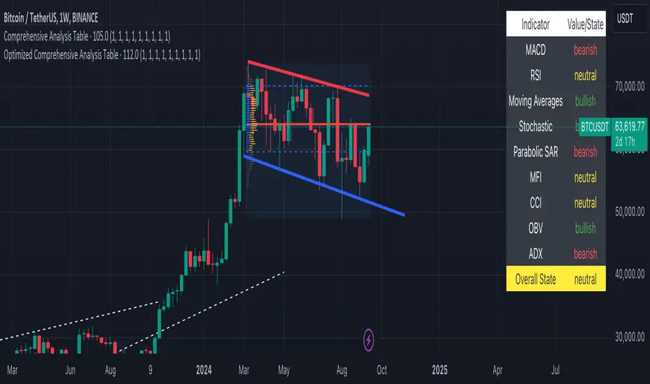
Optimized Comprehensive Analysis Table# Enhanced Comprehensive Analysis Table
This advanced indicator provides a holistic view of market sentiment by analyzing multiple technical indicators simultaneously. It's designed to give traders a quick, at-a-glance summary of market conditions across various timeframes and analysis methods.
## Key Features:
- Analyzes 9 popular technical indicators
- Weighted voting system for overall market sentiment
- Customizable indicator weights
- Clear, color-coded table display
## Indicators Analyzed:
1. MACD (Moving Average Convergence Divergence)
2. RSI (Relative Strength Index)
3. Moving Averages (50, 100, 200-period)
4. Stochastic Oscillator
5. Parabolic SAR
6. MFI (Money Flow Index)
7. CCI (Commodity Channel Index)
8. OBV (On Balance Volume)
9. ADX (Average Directional Index)
## How It Works:
Each indicator's signal is calculated and classified as bullish, bearish, or neutral. These signals are then weighted according to user-defined inputs. The weighted votes are summed to determine an overall market sentiment.
## Interpretation:
- The table displays the state of each indicator and the overall market sentiment.
- Green indicates bullish conditions, red bearish, and yellow neutral.
- The "Overall State" row at the bottom provides a quick summary of the combined analysis.
## Customization:
Users can adjust the weight of each indicator to fine-tune the analysis according to their trading strategy or market conditions.
This indicator is ideal for traders who want a comprehensive overview of market conditions without having to monitor multiple indicators separately. It's particularly useful for confirming trade setups, identifying potential trend reversals, and managing risk.
Note: This indicator is meant to be used as part of a broader trading strategy. Always combine with other forms of analysis and proper risk management.
Cerca negli script per "Table"
Time Matrix TableICT stresses time and liquidity levels in his teachings. This table helps to easily locate these key Time-based price levels. You can use these levels to determine your directional bias and to help generate your narrative for where the market is going.
This indicator creates a table that gives you the price for the following liquidity levels:
PDO - Previous Day Open
PDH - Previous Day High
PDL - Previous Day Low
PDC - Previous Day Close
PDEQ - Equilibrium of the previous day's range. (Calculated by math.abs(((pdh-pdl)/2)+pdl))
PWH - Previous Week High
PWL - Previous Week Low
PDH2 - Two Days Back High
PDL2 - Two Days Back Low
PDH3 - Three Days Back High
PDL3 - Three Days Back Low
And gives you the opening price for the following times:
Daily Open - 6:00pm open for current session
1:30 AM
3:00 AM
4:00 AM
Midnight Open
6:00 AM
7:30 AM
8:30 AM
NY Open
10:00 AM
12:00 PM
NY PM - 1:30pm
2:00 PM
The levels are sorted descending in price in the table, with the background colored based on their relation to price. The prices are also plotted on the chart based on the range you specify in relation to the current price. These lines are also colored based on their relation to price.
This indicator does not give you anything but the price at a specific time, you must determine your own bias and narrative based on the levels that are given.

Time & Sales (Tape) [By MUQWISHI]▋ INTRODUCTION :
The “Time and Sales” (Tape) indicator generates trade data, including time, direction, price, and volume for each executed trade on an exchange. This information is typically delivered in real-time on a tick-by-tick basis or lower timeframe, providing insights into the traded size for a specific security.
_______________________
▋ OVERVIEW:
_______________________
▋ Volume Dynamic Scale Bar:
It's a way for determining dominance on the time and sales table, depending on the selected length (number of rows), indicating whether buyers or sellers are in control in selected length.
_______________________
▋ INDICATOR SETTINGS:
#Section One: Table Settings
#Section Two: Technical Settings
(1) Implement By: Retrieve data by
(1A) Lower Timeframe: Fetch data from the selected lower timeframe.
(1B) Live Tick: Fetch data in real-time on a tick-by-tick basis, capturing data as soon as it's observed by the system.
(2) Length (Number of Rows): User able to select number of rows.
(3) Size Type: Volume OR Price Volume.
_____________________
▋ COMMENT:
The values in a table should not be taken as a major concept to build a trading decision.
Please let me know if you have any questions.
Thank you.

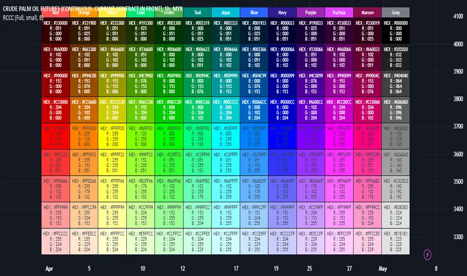
RGB Color Codes Chart█ OVERVIEW
This indicator is an educational indicator to make pine coders easier to input color code.
Color code displayed either in hex or rgb code or both.
█ INSPIRATIONS
RGB Color Codes Chart
Table Color For Pairing Black And White
█ FEATURES
Hover table cell to see all properties of color such as Hex code and RGB code via tooltip.
Cell can be show either Full, HEX, RGB, R, G, B or na.
█ LIMITATION
This code does not consider usage of color.new()
█ CONSIDERATION
Code consideration to be used such as color.r(), color.g(), color.b() and color.rgb()
█ EXAMPLE OF USAGE / EXPLAINATION
Crossing TableCrossing Table V1
I created this indicator as it had been asked for a number of times to create a crossover/under table screen and here it is!!!
The indicator is set up to be selected from SMA, EMA and Volume.
The SMA is defaulted to 2/10 but it is customizable to whatever SMA you choose to use.
Volume is based off a volume formula and the volume settings in the indicators settings, and the table will show either buyers/sellers on the last candle on the volume in the settings.
Just like the SMA the EMA option will be based off the default value of 5/13 but can be customized to your choosing.
If there are any question or comments just let me know :)

Performance Tablethis scrip is modified of Performance Table () of TradingView user @BeeHolder = Thank u very much.
-
@BeeHolder formula is based on daily basis,
but my calculation is based on respective day, week and month.
-
The formula of the calculation is (Current Close - Previous Close) * 100 / Previous Close, where Past value is:
1D = close 1 day before
5D = close 5 day before
1W - close 1 week before
4W = close 4 week before
1M - close 1 month before
3M - close 3 month before
6M - close 6 month before
12M - close 12 month before
52W - close 52 week before
Also table position cane be set.
thank you all
-

[HELPER] Math Constant Helper█ OVERVIEW
This indicator is to show constant in table using built-in math name space, coded in latest Pine Script version 5.
█ CREDITS
Credits to PineCoders.
█ FEATURES
- Display table by changing table position, font size and color.

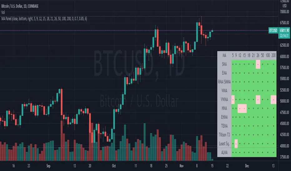
Moving Average PanelThis indicator calculates many different moving averages and displays whether they are increasing or decreasing as a panel/table instead of a plot. Rows/columns can be removed from the table as needed in the options menu, there is also a mobile friendly/compact option as well as a location option.
Note: This script is large and may take a few moments to load.
Note: If there is not enough data, will default to bearish/decreasing.
Value Added
This is the most complete and transparent moving average panel/table indicator. Unlike things such as the Technical Ratings, you can see what components are increasing or decreasing.
There may be some advantage in judging if a trend is likely to reverse or not based on the MA's with less lag.
Good for quick screening of charts.
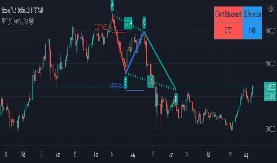
AB=CD Reciprocal Ratios Table (Source Code)This table indicator was intended as helper / reference for using ABCD Pattern.
Indikator berjadual bertujuan sebagai bantuan / rujukan untuk kegunaan ABCD Pattern.
The values shown in table was based on Harmonic Trading : Volume One book written by Scott M Carney.
Details of value, refer Chapter 4 : The AB=CD Pattern (Page 41).
These values are known as AB=CD Reciprocal Ratios.
Nilai yang ditunjukkan dalam jadual adalah berdasarkan buku Harmonic Trading : Volume One ditulis oleh Scott M Carney.
Nilai secara menyeluruh, rujuk Chapter 4 : The AB=CD Pattern (Muka surat 41).
Nilai berikut dipanggil sebagai AB=CD Reciprocal Ratios
Indicator features :
1. List AB=CD Reciprocal Ratios.
2. Font size small for mobile app and font size normal for desktop.
Kemampuan indikator :
1. Senarai AB=CD Reciprocal Ratio.
2. Saiz font kecil untuk mobile app dan saiz size normal untuk desktop.
FAQ
1. Credits / Kredit
Scott M Carney,
2. Code Usage / Penggunaan Kod
Free to use for personal usage but credits are most welcomed especially for credits to Scott M Carney/
Bebas untuk kegunaan peribadi tetapi kredit adalah amat dialu-alukan terutamanya kredit kepada Scott M Carney.
Settings with appropriate value.
Setting dengan nilai yang sesuai.
Default Settings.
Setting asal.
Settings with different table position.
Setting dengan posisi jadual yang berbeza.
⏰Forex Market Clock Table (DST Auto)⏰ Forex Market Clock Table (DST Auto)
Keep track of key forex session times with this clean, real-time table showing local time, market status (open/closed), and automatic Daylight Saving Time (DST) adjustments for Sydney, Tokyo, London, and New York. Displays countdowns to session open/close and highlights weekends. Fully customizable position, colors, and text size—perfect for multi-session traders.

Turtle System 1 Long & Short (Donchian + N-Stop) + MTF Table V6 Turtle Trading Long & Short (System 1 – 20/10 Donchian + True 2N Trailing Stop) + Multi-Timeframe Dashboard – Pine Script v6This indicator is a 100 % faithful implementation of the famous original Turtle Trading System 1 (Richard Dennis & William Eckhardt) with the following genuine rules:Entry: 20-period Donchian Channel breakout (using the high/low of the previous completed bars only → )
Exit: Classic 10-period Donchian opposite breakout OR hit of the volatility-based stop
Risk Management: True 2N trailing stop (N = 20-period ATR). The stop is pulled tighter on every new favorable extreme (real Turtle trailing – not fixed!)
Fully dynamic position tracking (Long / Short / Flat) on the chart’s timeframe
Visual signals: green/red triangles for entries, diamonds for exits, trailing stop line, entry labels with current N and stop price
Unique Feature – Multi-Timeframe (MTF) Status Table
A clean table in the top-right corner instantly shows the current Turtle position status on five higher timeframes simultaneously:Turtle MTF
1H
4H
8H
1D
1W
Status
LONG / SHORT / FLAT (color-coded)
This allows you to see at a glance whether higher timeframes are already in a Turtle trend – perfect for trend confirmation, filtering, or multi-timeframe trading.Key Visual ElementsLime upper Donchian line (20-period high)
Red lower Donchian line (10-period low)
Gray channel fill
Fuchsia trailing 2N stop line (moves only in favorable direction)
Entry labels showing current N-value and exact stop price
Arrows and diamonds for entries/exits
Alerts
Two ready-to-use alert conditions:“Turtle Long Entry”
“Turtle Short Entry”
Works on any market and any chart timeframe (stocks, forex, futures, crypto).
Completely written and tested in Pine Script version 6.A true, clean, no-nonsense Turtle System 1 with real trailing volatility stops and a powerful higher-timeframe dashboard – exactly how the original Turtles traded (only better visualized)! Enjoy the trends!

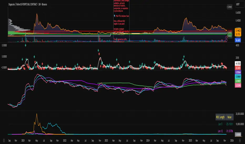
ROC x4 (Multi-Period Overlay) + Table📈 ROC x4 (Multi-Period Momentum Suite) + Compact Table
A clean, powerful momentum indicator that overlays four Rate-of-Change (ROC) periods inside a single pane — without needing to stack multiple separate indicators.
This script is designed for traders who use multi-timeframe momentum confirmation, trend strength validation, and early detection of rotation, compression, or expansion in price behavior.
🔍 What This Indicator Does
Plots 4 different ROC lengths in one panel
Includes a compact real-time ROC table that fits even in small panes
Tracks momentum shifts, trend acceleration, slowdowns, and regime transitions
Allows manual input for all 4 ROC lengths
Optional smoothing to reduce noise
Zero-line toggle for momentum direction clarity
Perfect for traders who want to monitor short-term, mid-term, and long-term ROC simultaneously.
EMA H/L 20-50 Table + RSI - KHALID ALADDIN🧾 Description
EMA H/L 20-50 Table + RSI — by Khalid Aladdin
A clean and minimal indicator designed for traders and analysts who prefer a quick glance at essential EMA values without any extra clutter on the chart.
📊 Features:
Displays precise values of EMA20 (High & Low) and EMA50 (High & Low) in a compact table below the chart.
Automatically updates values based on the current timeframe.
Includes RSI reading for momentum tracking.
Large, clear text with dark-theme friendly colors.
No lines or drawings — only a clean data panel.
✅ Perfect for:
Technical analysts, swing traders, and long-term investors who want an uncluttered view of trend levels and momentum strength.

USD Session 8FX - LDN & NY (TF-invariant, Live + Table)What it is
A USD strength/weakness meter for the London (08:00–08:45) or New York (15:30–16:00/16:15) session. It blends the movement of 8 markets—EURUSD, GBPUSD, AUDUSD, NZDUSD, USDCHF, USDCAD, USDJPY, XAUUSD—into one Score that is timeframe-invariant (it uses a 1-minute “boundary TF” under the hood so changing chart TF doesn’t change the math).
Core logic (simple)
During the chosen session window, it records each symbol’s start and live end prices, computes returns, optionally normalizes by ATR (volatility), applies your weights, and averages anti-USD (EUR/GBP/AUD/NZD/XAU) vs USD-base (CHF/CAD/JPY) groups.
The final Score is the normalized sum of weighted contributions:
Score > 0 → “USD Strong”
Score < 0 → “USD Weak”
At the session close it freezes (“Locked”) the results so you can review them later.
What you see
Main plot: the USD Score line (with a 0 baseline).
Optional lines: Anti-USD average vs USD-base average (post-normalization, pre-weights).
Session background shading (London silver, New York aqua).
Live table with:
Each symbol’s % change, its weight, and its contribution to the Score.
TOP badges for the two biggest drivers (by absolute contribution).
A Side column (only for the two TOPs) showing BUY/SELL aligned with the USD verdict (e.g., if USD Strong → SELL anti-USD pairs like EURUSD, BUY USD-base like USDCHF).
Verdict row with USD Strong/Weak, the Score value, the window text, and whether you’re LIVE / CLOSED / FROZEN.
Trade Gate panel:
Shows Verdict (USD Strong/Weak), Bias OK/weak (|Score| vs your threshold), Top-1/Top-2 VWAP checks, an overall GATE: OK/NO, and an Entry hint string (e.g., “SELL EURUSD, BUY USDCHF”) when conditions align.
VWAP “Trade Gate”
It confirms alignment between the USD bias and price vs VWAP for the top movers:
If USD Strong: anti-USD symbols should be below VWAP (short bias), USD-base symbols above VWAP (long bias).
If USD Weak: the opposite.
Gate = OK only if |Score| ≥ minAbsScore and at least one of the two TOP symbols is on the correct side of VWAP.
Tip: set vwapTF to an intraday value (“1”, “5”, “15”) for reliable VWAP on higher-TF charts.
Alerts
At session close: “USD Strong/Weak – session close”.
Live threshold: alerts when |Score| crosses your intraday threshold up/down.
Entry hint (Gate OK): triggers when the Gate flips from NO → OK inside the window.
If you create an alert of type “Any alert() function call”, you also get a dynamic message like:
ENTRY HINT • Hint: SELL EURUSD, BUY USDCHF
Key inputs you can tweak
Session: London vs New York; NY end time 16:00 or 16:15.
Timezone: default Europe/Tirane.
Boundary TF: default “1” (keeps the indicator TF-invariant).
minAbsScore: sensitivity threshold for “Bias OK”.
ATR normalization (len): stabilizes comparisons across different volatility regimes.
VWAP settings: toggle panel and set vwapTF.
How to use (playbook)
Choose the session (e.g., New York 15:30–16:15), keep Boundary TF = 1.
If you’re on a higher-TF chart, set vwapTF = "1" or "5".
Watch Score and Verdict; when |Score| ≥ minAbsScore, bias is meaningful.
Check Top-1/Top-2 and the Trade Gate:
If Gate = OK, use the Entry hint (e.g., “SELL EURUSD, BUY USDCHF”) as the aligned idea.
Use your own execution rules (e.g., structure, risk, stops) on the suggested symbols.
After close, review the Frozen table to validate behavior and refine thresholds/weights.
Notes & edge cases
If some markets are illiquid/holiday, a few returns may be na; the script handles that gracefully.
If ta.vwap is na on high TFs, the Gate will simply not confirm—set vwapTF intraday.
You can customize weights (e.g., reduce XAUUSD to -0.3 or similar) to suit your basket philosophy.
If you want, I can add toggles to show Side for all 8 symbols, or print a one-line summary (e.g., “USD Strong • Score 0.23 • Gate OK • SELL EURUSD, BUY USDCHF”) in the top-left of the pane.

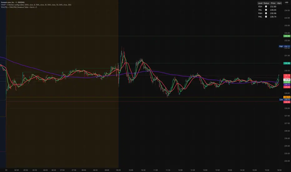
PDH/PDL + PMH/PML Breakout Table + Alerts + 🔔PDH/PDL now come exclusively from the previous day's RTH (9:30–4:00 PM ET) — they no longer include premarket. This avoids the confusion we encountered.
PMH/PML are calculated only during the premarket period (4:00–9:30 AM ET) of the current day.
Employment emojis: 🟢 (upward breakout for PDH/PMH), 🔴 (downward breakout for PDL/PML), ⚪ (no breakout).
The table displays three columns: Level | Status | Price. If you'd like the table to have a different size/position/color, just adjust it quickly.
Weinstein Stage Analyzer — Table Only (more padding)What it does
This indicator applies Stan Weinstein’s Stage Analysis (Stages 1–4) and presents the result in a clean, compact table only—no lines, labels, or overlays. It shows:
• Previous Stage
• Current Stage (with Early / Mature / Late tag)
• Duration (how long price has been in the current stage, in HTF bars)
• Sentiment (Bullish / Bearish / Balanced / Cautious, derived from stage & maturity)
Timeframe-aware logic
• Weekly charts: classic 30-period MA (Weinstein’s original 30-week concept).
• Daily & Intraday: computed on Daily 150 as a practical daily translation of the 30-week idea.
• Monthly: ~7-period MA (~30 weeks ≈ 7 months).
The stage classification itself is evaluated on this HTF context and then displayed on your active chart.
EMA/SMA toggle
Choose EMA (default) or SMA for the trend line used in stage detection.
How stages are decided (practical rules)
• Stage 2 (Advance): MA rising with price above an upper band.
• Stage 4 (Decline): MA falling with price below a lower band.
• Flat MA zones become Stage 1 (Base) or Stage 3 (Top) depending on the prior trend.
“Maturity” tags (Early/Mature/Late) come from run length and extension beyond the band.
Inputs you can tweak
• MA Type: EMA / SMA
• Price Band (±%) and Slope Threshold to tighten/loosen stage flips
• Maturity thresholds: min/max bars & late-extension %
Notes
• Duration is for the entire current stage (e.g., total time in Stage 4), not just the maturity slice.
• A Top Padding Rows input is included to nudge the table lower if it overlaps your OHLC readout.
Disclaimer
For educational use only. Not financial advice. Always confirm with your own analysis, risk management, and market context.

Trend Display Table (with Change Alerts)📌 Indicator: Trend Display Table (with Change Alerts)
This indicator helps identify trend direction based on a 15-minute 20 SMA compared against a 10 EMA applied to that SMA.
Trend Logic:
Bullish → 20 SMA crosses above 10 EMA (on SMA values)
Bearish → 20 SMA crosses below 10 EMA (on SMA values)
Neutral → No crossover (trend continues from previous state)
Display:
A compact trend table appears on the chart (top-right), showing the current trend with customizable colors, font size, and background.
Alerts:
Alerts are triggered only when the trend changes (from Bullish → Bearish or Bearish → Bullish).
This prevents repeated alerts on every bar.
✅ Useful for:
Confirming higher timeframe trend bias
Filtering trades in choppy markets
Getting notified instantly when the trend flips

RSI Z‑Score + TableRSI Z-Score + Table
This script calculates the Z-Score of the RSI (Relative Strength Index), which standardizes RSI based on its own recent history.
What It Shows:
RSI Z-Score = (Current RSI - Mean RSI) / Standard Deviation
This tells you how extreme the current RSI is compared to its historical values.
A table displays:
Current RSI
Rolling Mean
RSI Z-Score
How to Use:
Z-Score > +2 = Statistically overbought
Z-Score < -2 = Statistically oversold
Use it to time reversals or overextension in RSI behavior.
🔒 Based on rolling lookback window — fully customizable.
Author:
Tags: #RSI #ZScore #Momentum #StatisticalEdge #MeanReversion #Crypto

SG CBC Table - Full 10min & 2minBased on SG CBC Table has 10 min and 2 min CBC status and GC. Also customizable table colors of the background can be changed or made transparent. Indicator Updates every 10 minutes on a 10 minute chart and every 2 minutes on a 2 minute chart

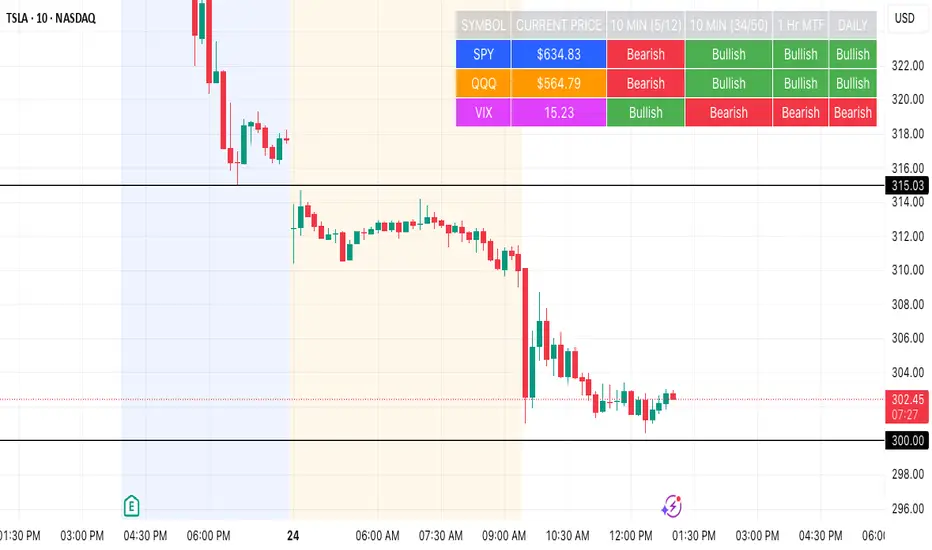
SPY, QQQ, VIX - Multi TF Trend Table***CURRENTLY IN BACKTESTING PHASE***
This TradingView script creates a real-time multi-timeframe trend status table for SPY, QQQ, and VIX using the Ripster-style EMA cloud logic.
🔍 What It Shows:
Current Price (1 Min): Live snapshot of each symbol.
10min Trend (5/12 EMA): Short-term momentum.
10min Trend (34/50 EMA): Intermediate-term direction.
1 Hour Trend: Higher timeframe trend.
Daily Trend: Long-term trend using 5/12 and 34/55 EMA alignment.
Each cell is color-coded:
✅ Green = Bullish
❌ Red = Bearish
Yellow can be used for neutral if customized.
⚙️ How It Works:
Uses request.security() to pull multi-timeframe EMA values for each symbol.
Compares fast/slow EMAs to determine bullish or bearish alignment.
The table is refreshed live and placed in a corner of your choice.
✅ Ideal For:
Trend traders using Ripster EMA clouds
SPY/QQQ/VIX correlation watchers
Traders seeking real-time trend clarity across multiple timeframes

SPY, QQQ, VIX Status TableBased on Ripster EMA and 1 hour MTF Clouds, this custom TradingView indicator displays a visual trend status table for SPY, QQQ, and VIX using multiple timeframes and EMA-based logic to be used on any stock ticker.
🔍 Key Features:
✅ Tracks 3 symbols: SPY, QQQ, and VIX
✅ Multiple trend conditions:
10-min (5/12 EMA) Ripster cloud trend
10-min (34/50 EMA) Ripster cloud trend
1-Hour Multi-Timeframe Ripster EMA trend
Daily open/close trend
✅ Color-coded trend strength:
🟩 Green = Bullish
🟥 Red = Bearish
🟨 Yellow = Sideways
✅ TO save screen space, customizations available:
Show/hide individual rows (SPY, QQQ, VIX)
Show/hide any trend column (10m, 1H MTF, Daily)
Change header/background colors and font color
Bold white top row for readability
✅ Auto-updating table appears on your chart, top-right
This tool is great for active traders looking to quickly scan short-term and longer-term momentum in key market instruments without having to go back and forth market charts.
PCR tableOverview
This indicator displays a multi-period table of forward-looking price projections. It combines normalized directional momentum (Positive Change Ratio, PCR) with volatility (ATR) and presents a forecast for upcoming time intervals, adjusted for your local UTC offset.
Concepts & Calculations
Positive Change Ratio (PCR):
((total positive change)/(total change)-0.5)*2, producing a value between –100 and +100.
Synthetic ATR: Calculates average true range over the same lookbacks to capture volatility.
PCR × ATR: Forms a volatility-weighted directional forecast, indicating expected move magnitude.
Future Price Projection: Adds PCR × ATR value to current close to estimate future price at each lookahead interval.
Table Layout
There are 12 forecast horizons—1× to 12× the chart timeframe (e.g., minutes, hours, days). Each row displays:
1. Future Time: Timestamp of each projection (adjustable via UTC offset)
2. PCR: Directional bias per period (–1 to +1)
3. PCR × ATR: E xpected move magnitude
4. Future Price: Close + (PCR × ATR)
High and low PCR×ATR rows are highlighted green for minimum value in the price forecast (buy signal) or red for maximum value in the price forecast (sell signal).
How to Use
1. Set UTC offset to your time zone for accurate future timestamps.
2. View PCR to assess bullish (positive) or bearish (negative) momentum.
3. Use PCR × ATR to estimate move strength and direction.
4. Reference Future Price for potential levels over upcoming intervals, and for buy and sell signals.
Limitations & Disclaimers
* This model uses linear extrapolation based on recent price behavior. It does not guarantee future prices.
* It uses only current bar data and no lookahead logic—compliant with Pine Script rules.
* Designed for analytical insight, not as an automated signal or trade executor.
* Best used on standard bar/candle charts (avoid non-standard types like Heikin‑Ashi or Renko).
