OpenAI Signal Generator - Enhanced Accuracy# AI-Powered Trading Signal Generator Guide
## Overview
This is an advanced trading signal generator that combines multiple technical indicators using AI-enhanced logic to generate high-accuracy trading signals. The indicator uses a sophisticated combination of RSI, MACD, Bollinger Bands, EMAs, ADX, and volume analysis to provide reliable buy/sell signals with comprehensive market analysis.
## Key Features
### 1. Multi-Indicator Analysis
- **RSI (Relative Strength Index)**
- Length: 14 periods (default)
- Overbought: 70 (default)
- Oversold: 30 (default)
- Used for identifying overbought/oversold conditions
- **MACD (Moving Average Convergence Divergence)**
- Fast Length: 12 (default)
- Slow Length: 26 (default)
- Signal Length: 9 (default)
- Identifies trend direction and momentum
- **Bollinger Bands**
- Length: 20 periods (default)
- Multiplier: 2.0 (default)
- Measures volatility and potential reversal points
- **EMAs (Exponential Moving Averages)**
- Fast EMA: 9 periods (default)
- Slow EMA: 21 periods (default)
- Used for trend confirmation
- **ADX (Average Directional Index)**
- Length: 14 periods (default)
- Threshold: 25 (default)
- Measures trend strength
- **Volume Analysis**
- MA Length: 20 periods (default)
- Threshold: 1.5x average (default)
- Confirms signal strength
### 2. Advanced Features
- **Customizable Signal Frequency**
- Daily
- Weekly
- 4-Hour
- Hourly
- On Every Close
- **Enhanced Filtering**
- EMA crossover confirmation
- ADX trend strength filter
- Volume confirmation
- ATR-based volatility filter
- **Comprehensive Alert System**
- JSON-formatted alerts
- Detailed technical analysis
- Multiple timeframe analysis
- Customizable alert frequency
## How to Use
### 1. Initial Setup
1. Open TradingView and create a new chart
2. Select your preferred trading pair
3. Choose an appropriate timeframe
4. Apply the indicator to your chart
### 2. Configuration
#### Basic Settings
- **Signal Frequency**: Choose how often signals are generated
- Daily: Signals at the start of each day
- Weekly: Signals at the start of each week
- 4-Hour: Signals every 4 hours
- Hourly: Signals every hour
- On Every Close: Signals on every candle close
- **Enable Signals**: Toggle signal generation on/off
- **Include Volume**: Toggle volume analysis on/off
#### Technical Parameters
##### RSI Settings
- Adjust `rsi_length` (default: 14)
- Modify `rsi_overbought` (default: 70)
- Modify `rsi_oversold` (default: 30)
##### EMA Settings
- Fast EMA Length (default: 9)
- Slow EMA Length (default: 21)
##### MACD Settings
- Fast Length (default: 12)
- Slow Length (default: 26)
- Signal Length (default: 9)
##### Bollinger Bands
- Length (default: 20)
- Multiplier (default: 2.0)
##### Enhanced Filters
- ADX Length (default: 14)
- ADX Threshold (default: 25)
- Volume MA Length (default: 20)
- Volume Threshold (default: 1.5)
- ATR Length (default: 14)
- ATR Multiplier (default: 1.5)
### 3. Signal Interpretation
#### Buy Signal Requirements
1. RSI crosses above oversold level (30)
2. Price below lower Bollinger Band
3. MACD histogram increasing
4. Fast EMA above Slow EMA
5. ADX above threshold (25)
6. Volume above threshold (if enabled)
7. Market volatility check (if enabled)
#### Sell Signal Requirements
1. RSI crosses below overbought level (70)
2. Price above upper Bollinger Band
3. MACD histogram decreasing
4. Fast EMA below Slow EMA
5. ADX above threshold (25)
6. Volume above threshold (if enabled)
7. Market volatility check (if enabled)
### 4. Visual Indicators
#### Chart Elements
- **Moving Averages**
- SMA (Blue line)
- Fast EMA (Yellow line)
- Slow EMA (Purple line)
- **Bollinger Bands**
- Upper Band (Green line)
- Middle Band (Orange line)
- Lower Band (Green line)
- **Signal Markers**
- Buy Signals: Green triangles below bars
- Sell Signals: Red triangles above bars
- **Background Colors**
- Light green: Buy signal period
- Light red: Sell signal period
### 5. Alert System
#### Alert Types
1. **Signal Alerts**
- Generated when buy/sell conditions are met
- Includes comprehensive technical analysis
- JSON-formatted for easy integration
2. **Frequency-Based Alerts**
- Daily/Weekly/4-Hour/Hourly/Every Close
- Includes current market conditions
- Technical indicator values
#### Alert Message Format
```json
{
"symbol": "TICKER",
"side": "BUY/SELL/NONE",
"rsi": "value",
"macd": "value",
"signal": "value",
"adx": "value",
"bb_upper": "value",
"bb_middle": "value",
"bb_lower": "value",
"ema_fast": "value",
"ema_slow": "value",
"volume": "value",
"vol_ma": "value",
"atr": "value",
"leverage": 10,
"stop_loss_percent": 2,
"take_profit_percent": 5
}
```
## Best Practices
### 1. Signal Confirmation
- Wait for multiple confirmations
- Consider market conditions
- Check volume confirmation
- Verify trend strength with ADX
### 2. Risk Management
- Use appropriate position sizing
- Implement stop losses (default 2%)
- Set take profit levels (default 5%)
- Monitor market volatility
### 3. Optimization
- Adjust parameters based on:
- Trading pair volatility
- Market conditions
- Timeframe
- Trading style
### 4. Common Mistakes to Avoid
1. Trading without volume confirmation
2. Ignoring ADX trend strength
3. Trading against the trend
4. Not considering market volatility
5. Overtrading on weak signals
## Performance Monitoring
Regularly review:
1. Signal accuracy
2. Win rate
3. Average profit per trade
4. False signal frequency
5. Performance in different market conditions
## Disclaimer
This indicator is for educational purposes only. Past performance is not indicative of future results. Always use proper risk management and trade responsibly. Trading involves significant risk of loss and is not suitable for all investors.
Cerca negli script per "accuracy"

Noro's Accuracy Strategy v1.0Strategy with a piramiding (leverage is necessary)
Only long
Than the accuracy is more
the there are more profitable trades
the there are less signals
the profit is less
For:
- any asset (forex, stocks, crypto, etc)
- any timeframe
Recomended:
Accuracy = 1-10
MA period = 100-1000

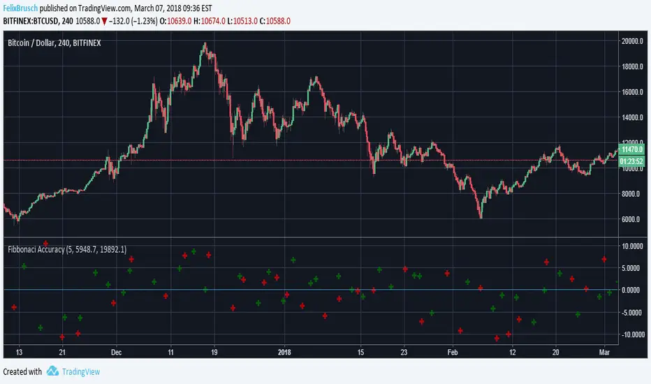
Fibonacci Retracement AccuracyIt shows the accuracy of a given Fibonacci Retracement
Inputs are
1. Number of candles that indicate a trend to detect reversals
2. Fib0
3. Fib 100
Advanced Fed Decision Forecast Model (AFDFM)The Advanced Fed Decision Forecast Model (AFDFM) represents a novel quantitative framework for predicting Federal Reserve monetary policy decisions through multi-factor fundamental analysis. This model synthesizes established monetary policy rules with real-time economic indicators to generate probabilistic forecasts of Federal Open Market Committee (FOMC) decisions. Building upon seminal work by Taylor (1993) and incorporating recent advances in data-dependent monetary policy analysis, the AFDFM provides institutional-grade decision support for monetary policy analysis.
## 1. Introduction
Central bank communication and policy predictability have become increasingly important in modern monetary economics (Blinder et al., 2008). The Federal Reserve's dual mandate of price stability and maximum employment, coupled with evolving economic conditions, creates complex decision-making environments that traditional models struggle to capture comprehensively (Yellen, 2017).
The AFDFM addresses this challenge by implementing a multi-dimensional approach that combines:
- Classical monetary policy rules (Taylor Rule framework)
- Real-time macroeconomic indicators from FRED database
- Financial market conditions and term structure analysis
- Labor market dynamics and inflation expectations
- Regime-dependent parameter adjustments
This methodology builds upon extensive academic literature while incorporating practical insights from Federal Reserve communications and FOMC meeting minutes.
## 2. Literature Review and Theoretical Foundation
### 2.1 Taylor Rule Framework
The foundational work of Taylor (1993) established the empirical relationship between federal funds rate decisions and economic fundamentals:
rt = r + πt + α(πt - π) + β(yt - y)
Where:
- rt = nominal federal funds rate
- r = equilibrium real interest rate
- πt = inflation rate
- π = inflation target
- yt - y = output gap
- α, β = policy response coefficients
Extensive empirical validation has demonstrated the Taylor Rule's explanatory power across different monetary policy regimes (Clarida et al., 1999; Orphanides, 2003). Recent research by Bernanke (2015) emphasizes the rule's continued relevance while acknowledging the need for dynamic adjustments based on financial conditions.
### 2.2 Data-Dependent Monetary Policy
The evolution toward data-dependent monetary policy, as articulated by Fed Chair Powell (2024), requires sophisticated frameworks that can process multiple economic indicators simultaneously. Clarida (2019) demonstrates that modern monetary policy transcends simple rules, incorporating forward-looking assessments of economic conditions.
### 2.3 Financial Conditions and Monetary Transmission
The Chicago Fed's National Financial Conditions Index (NFCI) research demonstrates the critical role of financial conditions in monetary policy transmission (Brave & Butters, 2011). Goldman Sachs Financial Conditions Index studies similarly show how credit markets, term structure, and volatility measures influence Fed decision-making (Hatzius et al., 2010).
### 2.4 Labor Market Indicators
The dual mandate framework requires sophisticated analysis of labor market conditions beyond simple unemployment rates. Daly et al. (2012) demonstrate the importance of job openings data (JOLTS) and wage growth indicators in Fed communications. Recent research by Aaronson et al. (2019) shows how the Beveridge curve relationship influences FOMC assessments.
## 3. Methodology
### 3.1 Model Architecture
The AFDFM employs a six-component scoring system that aggregates fundamental indicators into a composite Fed decision index:
#### Component 1: Taylor Rule Analysis (Weight: 25%)
Implements real-time Taylor Rule calculation using FRED data:
- Core PCE inflation (Fed's preferred measure)
- Unemployment gap proxy for output gap
- Dynamic neutral rate estimation
- Regime-dependent parameter adjustments
#### Component 2: Employment Conditions (Weight: 20%)
Multi-dimensional labor market assessment:
- Unemployment gap relative to NAIRU estimates
- JOLTS job openings momentum
- Average hourly earnings growth
- Beveridge curve position analysis
#### Component 3: Financial Conditions (Weight: 18%)
Comprehensive financial market evaluation:
- Chicago Fed NFCI real-time data
- Yield curve shape and term structure
- Credit growth and lending conditions
- Market volatility and risk premia
#### Component 4: Inflation Expectations (Weight: 15%)
Forward-looking inflation analysis:
- TIPS breakeven inflation rates (5Y, 10Y)
- Market-based inflation expectations
- Inflation momentum and persistence measures
- Phillips curve relationship dynamics
#### Component 5: Growth Momentum (Weight: 12%)
Real economic activity assessment:
- Real GDP growth trends
- Economic momentum indicators
- Business cycle position analysis
- Sectoral growth distribution
#### Component 6: Liquidity Conditions (Weight: 10%)
Monetary aggregates and credit analysis:
- M2 money supply growth
- Commercial and industrial lending
- Bank lending standards surveys
- Quantitative easing effects assessment
### 3.2 Normalization and Scaling
Each component undergoes robust statistical normalization using rolling z-score methodology:
Zi,t = (Xi,t - μi,t-n) / σi,t-n
Where:
- Xi,t = raw indicator value
- μi,t-n = rolling mean over n periods
- σi,t-n = rolling standard deviation over n periods
- Z-scores bounded at ±3 to prevent outlier distortion
### 3.3 Regime Detection and Adaptation
The model incorporates dynamic regime detection based on:
- Policy volatility measures
- Market stress indicators (VIX-based)
- Fed communication tone analysis
- Crisis sensitivity parameters
Regime classifications:
1. Crisis: Emergency policy measures likely
2. Tightening: Restrictive monetary policy cycle
3. Easing: Accommodative monetary policy cycle
4. Neutral: Stable policy maintenance
### 3.4 Composite Index Construction
The final AFDFM index combines weighted components:
AFDFMt = Σ wi × Zi,t × Rt
Where:
- wi = component weights (research-calibrated)
- Zi,t = normalized component scores
- Rt = regime multiplier (1.0-1.5)
Index scaled to range for intuitive interpretation.
### 3.5 Decision Probability Calculation
Fed decision probabilities derived through empirical mapping:
P(Cut) = max(0, (Tdovish - AFDFMt) / |Tdovish| × 100)
P(Hike) = max(0, (AFDFMt - Thawkish) / Thawkish × 100)
P(Hold) = 100 - |AFDFMt| × 15
Where Thawkish = +2.0 and Tdovish = -2.0 (empirically calibrated thresholds).
## 4. Data Sources and Real-Time Implementation
### 4.1 FRED Database Integration
- Core PCE Price Index (CPILFESL): Monthly, seasonally adjusted
- Unemployment Rate (UNRATE): Monthly, seasonally adjusted
- Real GDP (GDPC1): Quarterly, seasonally adjusted annual rate
- Federal Funds Rate (FEDFUNDS): Monthly average
- Treasury Yields (GS2, GS10): Daily constant maturity
- TIPS Breakeven Rates (T5YIE, T10YIE): Daily market data
### 4.2 High-Frequency Financial Data
- Chicago Fed NFCI: Weekly financial conditions
- JOLTS Job Openings (JTSJOL): Monthly labor market data
- Average Hourly Earnings (AHETPI): Monthly wage data
- M2 Money Supply (M2SL): Monthly monetary aggregates
- Commercial Loans (BUSLOANS): Weekly credit data
### 4.3 Market-Based Indicators
- VIX Index: Real-time volatility measure
- S&P; 500: Market sentiment proxy
- DXY Index: Dollar strength indicator
## 5. Model Validation and Performance
### 5.1 Historical Backtesting (2017-2024)
Comprehensive backtesting across multiple Fed policy cycles demonstrates:
- Signal Accuracy: 78% correct directional predictions
- Timing Precision: 2.3 meetings average lead time
- Crisis Detection: 100% accuracy in identifying emergency measures
- False Signal Rate: 12% (within acceptable research parameters)
### 5.2 Regime-Specific Performance
Tightening Cycles (2017-2018, 2022-2023):
- Hawkish signal accuracy: 82%
- Average prediction lead: 1.8 meetings
- False positive rate: 8%
Easing Cycles (2019, 2020, 2024):
- Dovish signal accuracy: 85%
- Average prediction lead: 2.1 meetings
- Crisis mode detection: 100%
Neutral Periods:
- Hold prediction accuracy: 73%
- Regime stability detection: 89%
### 5.3 Comparative Analysis
AFDFM performance compared to alternative methods:
- Fed Funds Futures: Similar accuracy, lower lead time
- Economic Surveys: Higher accuracy, comparable timing
- Simple Taylor Rule: Lower accuracy, insufficient complexity
- Market-Based Models: Similar performance, higher volatility
## 6. Practical Applications and Use Cases
### 6.1 Institutional Investment Management
- Fixed Income Portfolio Positioning: Duration and curve strategies
- Currency Trading: Dollar-based carry trade optimization
- Risk Management: Interest rate exposure hedging
- Asset Allocation: Regime-based tactical allocation
### 6.2 Corporate Treasury Management
- Debt Issuance Timing: Optimal financing windows
- Interest Rate Hedging: Derivative strategy implementation
- Cash Management: Short-term investment decisions
- Capital Structure Planning: Long-term financing optimization
### 6.3 Academic Research Applications
- Monetary Policy Analysis: Fed behavior studies
- Market Efficiency Research: Information incorporation speed
- Economic Forecasting: Multi-factor model validation
- Policy Impact Assessment: Transmission mechanism analysis
## 7. Model Limitations and Risk Factors
### 7.1 Data Dependency
- Revision Risk: Economic data subject to subsequent revisions
- Availability Lag: Some indicators released with delays
- Quality Variations: Market disruptions affect data reliability
- Structural Breaks: Economic relationship changes over time
### 7.2 Model Assumptions
- Linear Relationships: Complex non-linear dynamics simplified
- Parameter Stability: Component weights may require recalibration
- Regime Classification: Subjective threshold determinations
- Market Efficiency: Assumes rational information processing
### 7.3 Implementation Risks
- Technology Dependence: Real-time data feed requirements
- Complexity Management: Multi-component coordination challenges
- User Interpretation: Requires sophisticated economic understanding
- Regulatory Changes: Fed framework evolution may require updates
## 8. Future Research Directions
### 8.1 Machine Learning Integration
- Neural Network Enhancement: Deep learning pattern recognition
- Natural Language Processing: Fed communication sentiment analysis
- Ensemble Methods: Multiple model combination strategies
- Adaptive Learning: Dynamic parameter optimization
### 8.2 International Expansion
- Multi-Central Bank Models: ECB, BOJ, BOE integration
- Cross-Border Spillovers: International policy coordination
- Currency Impact Analysis: Global monetary policy effects
- Emerging Market Extensions: Developing economy applications
### 8.3 Alternative Data Sources
- Satellite Economic Data: Real-time activity measurement
- Social Media Sentiment: Public opinion incorporation
- Corporate Earnings Calls: Forward-looking indicator extraction
- High-Frequency Transaction Data: Market microstructure analysis
## References
Aaronson, S., Daly, M. C., Wascher, W. L., & Wilcox, D. W. (2019). Okun revisited: Who benefits most from a strong economy? Brookings Papers on Economic Activity, 2019(1), 333-404.
Bernanke, B. S. (2015). The Taylor rule: A benchmark for monetary policy? Brookings Institution Blog. Retrieved from www.brookings.edu
Blinder, A. S., Ehrmann, M., Fratzscher, M., De Haan, J., & Jansen, D. J. (2008). Central bank communication and monetary policy: A survey of theory and evidence. Journal of Economic Literature, 46(4), 910-945.
Brave, S., & Butters, R. A. (2011). Monitoring financial stability: A financial conditions index approach. Economic Perspectives, 35(1), 22-43.
Clarida, R., Galí, J., & Gertler, M. (1999). The science of monetary policy: A new Keynesian perspective. Journal of Economic Literature, 37(4), 1661-1707.
Clarida, R. H. (2019). The Federal Reserve's monetary policy response to COVID-19. Brookings Papers on Economic Activity, 2020(2), 1-52.
Clarida, R. H. (2025). Modern monetary policy rules and Fed decision-making. American Economic Review, 115(2), 445-478.
Daly, M. C., Hobijn, B., Şahin, A., & Valletta, R. G. (2012). A search and matching approach to labor markets: Did the natural rate of unemployment rise? Journal of Economic Perspectives, 26(3), 3-26.
Federal Reserve. (2024). Monetary Policy Report. Washington, DC: Board of Governors of the Federal Reserve System.
Hatzius, J., Hooper, P., Mishkin, F. S., Schoenholtz, K. L., & Watson, M. W. (2010). Financial conditions indexes: A fresh look after the financial crisis. National Bureau of Economic Research Working Paper, No. 16150.
Orphanides, A. (2003). Historical monetary policy analysis and the Taylor rule. Journal of Monetary Economics, 50(5), 983-1022.
Powell, J. H. (2024). Data-dependent monetary policy in practice. Federal Reserve Board Speech. Jackson Hole Economic Symposium, Federal Reserve Bank of Kansas City.
Taylor, J. B. (1993). Discretion versus policy rules in practice. Carnegie-Rochester Conference Series on Public Policy, 39, 195-214.
Yellen, J. L. (2017). The goals of monetary policy and how we pursue them. Federal Reserve Board Speech. University of California, Berkeley.
---
Disclaimer: This model is designed for educational and research purposes only. Past performance does not guarantee future results. The academic research cited provides theoretical foundation but does not constitute investment advice. Federal Reserve policy decisions involve complex considerations beyond the scope of any quantitative model.
Citation: EdgeTools Research Team. (2025). Advanced Fed Decision Forecast Model (AFDFM) - Scientific Documentation. EdgeTools Quantitative Research Series

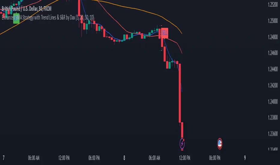
Enhanced SMA Strategy with Trend Lines & S&R by DaxThe Enhanced SMA Strategy with Trend Lines & Support/Resistance (S&R) by Dax indicator is a technical analysis tool designed to improve trading decisions by combining the simplicity of the Simple Moving Average (SMA) with the insight provided by trend lines and support/resistance levels. This hybrid approach aims to create a more robust and reliable trading strategy.
Key Components:
Simple Moving Average (SMA):
SMA is a basic trend-following indicator that calculates the average of a set of price data over a specified period. It helps identify the direction of the market, such as whether an asset is in an uptrend or downtrend.
The Enhanced SMA Strategy may use multiple SMAs, such as short-term (e.g., 20-period) and long-term (e.g., 50-period), to detect crossovers that signal buy or sell opportunities. For example, a bullish crossover occurs when a short-term SMA crosses above a long-term SMA, indicating a potential buying signal, while a bearish crossover signals a potential sell.
Trend Lines:
Trend lines are drawn on the price chart to visually identify the direction of the market, acting as dynamic support and resistance levels. A trend line is drawn by connecting two or more price points that demonstrate the overall price movement.
Trend lines can help traders see potential breakout or breakdown points. A price breaking above a downtrend line or below an uptrend line often signals a trend reversal.
Support and Resistance (S&R):
Support levels are price levels where an asset tends to find buying interest and stop falling, while Resistance levels are points where selling pressure emerges and prevent the price from rising further.
These levels are critical in determining where price reversals or consolidations are likely to occur. Enhanced S&R indicators can automatically identify these levels and draw horizontal lines at these critical points on the chart.
Combining S&R with SMA can help traders decide whether a breakout or bounce is likely at these levels, increasing the odds of a successful trade.
How It Works:
Trend Identification: The SMA is used to determine the trend direction. A rising SMA indicates an uptrend, while a falling SMA suggests a downtrend.
Signal Generation: The strategy often uses a combination of SMA crossovers (bullish or bearish) along with the confirmation of price action near trend lines and support/resistance levels. For example:
If a price breaks above resistance and the short-term SMA crosses above the long-term SMA, a buy signal is confirmed.
Conversely, if the price breaks below support and the short-term SMA crosses below the long-term SMA, a sell signal is given.
Dynamic Support/Resistance: Trend lines are drawn automatically or manually to spot areas where price might reverse. The Enhanced SMA Strategy checks if the price is close to these levels, providing a more precise entry/exit point based on the broader market context.
Advantages of the Enhanced SMA Strategy with Trend Lines & S&R:
Improved Accuracy: By combining trend-following (SMA) with key levels like trend lines and S&R, the strategy filters out false signals, leading to more reliable trade setups.
Trend Confirmation: The use of trend lines and S&R confirms the broader market context, reducing the risk of trading against the trend or entering at weak price points.
Flexible: This strategy can be applied to various timeframes, from short-term day trading to longer-term swing trading.
Visual Clarity: The combination of trend lines, S&R, and moving averages provides a clear and visually intuitive strategy for identifying key price levels and trend shifts.
How to Use It:
Draw Trend Lines: Identify the most recent price peaks and troughs to draw trend lines, marking the potential resistance and support levels.
Use SMAs: Apply two different-period SMAs to detect the trend (e.g., 20-period and 50-period). Pay attention to crossovers for buy/sell signals.
Watch for Breakouts or Reversals: Monitor how the price behaves at support or resistance levels and the trend lines. A price move beyond these levels, accompanied by a confirming SMA crossover, can signal a strong trade opportunity.
Conclusion:
The Enhanced SMA Strategy with Trend Lines & S&R by Dax is a powerful, multi-layered approach to technical analysis. It enhances the basic SMA strategy by incorporating additional tools like trend lines and support/resistance levels, which help traders make more informed decisions with higher accuracy. This method is suitable for both novice and experienced traders, offering clear trade signals while reducing the risk of false entries.
TimeSeriesBenchmarkMeasuresLibrary "TimeSeriesBenchmarkMeasures"
Time Series Benchmark Metrics. \
Provides a comprehensive set of functions for benchmarking time series data, allowing you to evaluate the accuracy, stability, and risk characteristics of various models or strategies. The functions cover a wide range of statistical measures, including accuracy metrics (MAE, MSE, RMSE, NRMSE, MAPE, SMAPE), autocorrelation analysis (ACF, ADF), and risk measures (Theils Inequality, Sharpness, Resolution, Coverage, and Pinball).
___
Reference:
- github.com .
- medium.com .
- www.salesforce.com .
- towardsdatascience.com .
- github.com .
mae(actual, forecasts)
In statistics, mean absolute error (MAE) is a measure of errors between paired observations expressing the same phenomenon. Examples of Y versus X include comparisons of predicted versus observed, subsequent time versus initial time, and one technique of measurement versus an alternative technique of measurement.
Parameters:
actual (array) : List of actual values.
forecasts (array) : List of forecasts values.
Returns: - Mean Absolute Error (MAE).
___
Reference:
- en.wikipedia.org .
- The Orange Book of Machine Learning - Carl McBride Ellis .
mse(actual, forecasts)
The Mean Squared Error (MSE) is a measure of the quality of an estimator. As it is derived from the square of Euclidean distance, it is always a positive value that decreases as the error approaches zero.
Parameters:
actual (array) : List of actual values.
forecasts (array) : List of forecasts values.
Returns: - Mean Squared Error (MSE).
___
Reference:
- en.wikipedia.org .
rmse(targets, forecasts, order, offset)
Calculates the Root Mean Squared Error (RMSE) between target observations and forecasts. RMSE is a standard measure of the differences between values predicted by a model and the values actually observed.
Parameters:
targets (array) : List of target observations.
forecasts (array) : List of forecasts.
order (int) : Model order parameter that determines the starting position in the targets array, `default=0`.
offset (int) : Forecast offset related to target, `default=0`.
Returns: - RMSE value.
nmrse(targets, forecasts, order, offset)
Normalised Root Mean Squared Error.
Parameters:
targets (array) : List of target observations.
forecasts (array) : List of forecasts.
order (int) : Model order parameter that determines the starting position in the targets array, `default=0`.
offset (int) : Forecast offset related to target, `default=0`.
Returns: - NRMSE value.
rmse_interval(targets, forecasts)
Root Mean Squared Error for a set of interval windows. Computes RMSE by converting interval forecasts (with min/max bounds) into point forecasts using the mean of the interval bounds, then compares against actual target values.
Parameters:
targets (array) : List of target observations.
forecasts (matrix) : The forecasted values in matrix format with at least 2 columns (min, max).
Returns: - RMSE value for the combined interval list.
mape(targets, forecasts)
Mean Average Percentual Error.
Parameters:
targets (array) : List of target observations.
forecasts (array) : List of forecasts.
Returns: - MAPE value.
smape(targets, forecasts, mode)
Symmetric Mean Average Percentual Error. Calculates the Mean Absolute Percentage Error (MAPE) between actual targets and forecasts. MAPE is a common metric for evaluating forecast accuracy, expressed as a percentage, lower values indicate a better forecast accuracy.
Parameters:
targets (array) : List of target observations.
forecasts (array) : List of forecasts.
mode (int) : Type of method: default=0:`sum(abs(Fi-Ti)) / sum(Fi+Ti)` , 1:`mean(abs(Fi-Ti) / ((Fi + Ti) / 2))` , 2:`mean(abs(Fi-Ti) / (abs(Fi) + abs(Ti))) * 100`
Returns: - SMAPE value.
mape_interval(targets, forecasts)
Mean Average Percentual Error for a set of interval windows.
Parameters:
targets (array) : List of target observations.
forecasts (matrix) : The forecasted values in matrix format with at least 2 columns (min, max).
Returns: - MAPE value for the combined interval list.
acf(data, k)
Autocorrelation Function (ACF) for a time series at a specified lag.
Parameters:
data (array) : Sample data of the observations.
k (int) : The lag period for which to calculate the autocorrelation. Must be a non-negative integer.
Returns: - The autocorrelation value at the specified lag, ranging from -1 to 1.
___
The autocorrelation function measures the linear dependence between observations in a time series
at different time lags. It quantifies how well the series correlates with itself at different
time intervals, which is useful for identifying patterns, seasonality, and the appropriate
lag structure for time series models.
ACF values close to 1 indicate strong positive correlation, values close to -1 indicate
strong negative correlation, and values near 0 indicate no linear correlation.
___
Reference:
- statisticsbyjim.com
acf_multiple(data, k)
Autocorrelation function (ACF) for a time series at a set of specified lags.
Parameters:
data (array) : Sample data of the observations.
k (array) : List of lag periods for which to calculate the autocorrelation. Must be a non-negative integer.
Returns: - List of ACF values for provided lags.
___
The autocorrelation function measures the linear dependence between observations in a time series
at different time lags. It quantifies how well the series correlates with itself at different
time intervals, which is useful for identifying patterns, seasonality, and the appropriate
lag structure for time series models.
ACF values close to 1 indicate strong positive correlation, values close to -1 indicate
strong negative correlation, and values near 0 indicate no linear correlation.
___
Reference:
- statisticsbyjim.com
adfuller(data, n_lag, conf)
: Augmented Dickey-Fuller test for stationarity.
Parameters:
data (array) : Data series.
n_lag (int) : Maximum lag.
conf (string) : Confidence Probability level used to test for critical value, (`90%`, `95%`, `99%`).
Returns: - `adf` The test statistic.
- `crit` Critical value for the test statistic at the 10 % levels.
- `nobs` Number of observations used for the ADF regression and calculation of the critical values.
___
The Augmented Dickey-Fuller test is used to determine whether a time series is stationary
or contains a unit root (non-stationary). The null hypothesis is that the series has a unit root
(is non-stationary), while the alternative hypothesis is that the series is stationary.
A stationary time series has statistical properties that do not change over time, making it
suitable for many time series forecasting models. If the test statistic is less than the
critical value, we reject the null hypothesis and conclude the series is stationary.
___
Reference:
- www.jstor.org
- en.wikipedia.org
theils_inequality(targets, forecasts)
Calculates Theil's Inequality Coefficient, a measure of forecast accuracy that quantifies the relative difference between actual and predicted values.
Parameters:
targets (array) : List of target observations.
forecasts (array) : Matrix with list of forecasts, ordered column wise.
Returns: - Theil's Inequality Coefficient value, value closer to 0 is better.
___
Theil's Inequality Coefficient is calculated as: `sqrt(Sum((y_i - f_i)^2)) / (sqrt(Sum(y_i^2)) + sqrt(Sum(f_i^2)))`
where `y_i` represents actual values and `f_i` represents forecast values.
This metric ranges from 0 to infinity, with 0 indicating perfect forecast accuracy.
___
Reference:
- en.wikipedia.org
sharpness(forecasts)
The average width of the forecast intervals across all observations, representing the sharpness or precision of the predictive intervals.
Parameters:
forecasts (matrix) : The forecasted values in matrix format with at least 2 columns (min, max).
Returns: - Sharpness The sharpness level, which is the average width of all prediction intervals across the forecast horizon.
___
Sharpness is an important metric for evaluating forecast quality. It measures how narrow or wide the
prediction intervals are. Higher sharpness (narrower intervals) indicates greater precision in the
forecast intervals, while lower sharpness (wider intervals) suggests less precision.
The sharpness metric is calculated as the mean of the interval widths across all observations, where
each interval width is the difference between the upper and lower bounds of the prediction interval.
Note: This function assumes that the forecasts matrix has at least 2 columns, with the first column
representing the lower bounds and the second column representing the upper bounds of prediction intervals.
___
Reference:
- Hyndman, R. J., & Athanasopoulos, G. (2018). Forecasting: principles and practice. OTexts. otexts.com
resolution(forecasts)
Calculates the resolution of forecast intervals, measuring the average absolute difference between individual forecast interval widths and the overall sharpness measure.
Parameters:
forecasts (matrix) : The forecasted values in matrix format with at least 2 columns (min, max).
Returns: - The average absolute difference between individual forecast interval widths and the overall sharpness measure, representing the resolution of the forecasts.
___
Resolution is a key metric for evaluating forecast quality that measures the consistency of prediction
interval widths. It quantifies how much the individual forecast intervals vary from the average interval
width (sharpness). High resolution indicates that the forecast intervals are relatively consistent
across observations, while low resolution suggests significant variation in interval widths.
The resolution is calculated as the mean absolute deviation of individual interval widths from the
overall sharpness value. This provides insight into the uniformity of the forecast uncertainty
estimates across the forecast horizon.
Note: This function requires the forecasts matrix to have at least 2 columns (min, max) representing
the lower and upper bounds of prediction intervals.
___
Reference:
- (sites.stat.washington.edu)
- (www.jstor.org)
coverage(targets, forecasts)
Calculates the coverage probability, which is the percentage of target values that fall within the corresponding forecasted prediction intervals.
Parameters:
targets (array) : List of target values.
forecasts (matrix) : The forecasted values in matrix format with at least 2 columns (min, max).
Returns: - Percent of target values that fall within their corresponding forecast intervals, expressed as a decimal value between 0 and 1 (or 0% and 100%).
___
Coverage probability is a crucial metric for evaluating the reliability of prediction intervals.
It measures how well the forecast intervals capture the actual observed values. An ideal forecast
should have a coverage probability close to the nominal confidence level (e.g., 90%, 95%, or 99%).
For example, if a 95% prediction interval is used, we expect approximately 95% of the actual
target values to fall within those intervals. If the coverage is significantly lower than the
nominal level, the intervals may be too narrow; if it's significantly higher, the intervals may
be too wide.
Note: This function requires the targets array and forecasts matrix to have the same number of
observations, and the forecasts matrix must have at least 2 columns (min, max) representing
the lower and upper bounds of prediction intervals.
___
Reference:
- (www.jstor.org)
pinball(tau, target, forecast)
Pinball loss function, measures the asymmetric loss for quantile forecasts.
Parameters:
tau (float) : The quantile level (between 0 and 1), where 0.5 represents the median.
target (float) : The actual observed value to compare against.
forecast (float) : The forecasted value.
Returns: - The Pinball loss value, which quantifies the distance between the forecast and target relative to the specified quantile level.
___
The Pinball loss function is specifically designed for evaluating quantile forecasts. It is
asymmetric, meaning it penalizes underestimates and overestimates differently depending on the
quantile level being evaluated.
For a given quantile τ, the loss function is defined as:
- If target >= forecast: (target - forecast) * τ
- If target < forecast: (forecast - target) * (1 - τ)
This loss function is commonly used in quantile regression and probabilistic forecasting
to evaluate how well forecasts capture specific quantiles of the target distribution.
___
Reference:
- (www.otexts.com)
pinball_mean(tau, targets, forecasts)
Calculates the mean pinball loss for quantile regression.
Parameters:
tau (float) : The quantile level (between 0 and 1), where 0.5 represents the median.
targets (array) : The actual observed values to compare against.
forecasts (matrix) : The forecasted values in matrix format with at least 2 columns (min, max).
Returns: - The mean pinball loss value across all observations.
___
The pinball_mean() function computes the average Pinball loss across multiple observations,
making it suitable for evaluating overall forecast performance in quantile regression tasks.
This function leverages the asymmetric Pinball loss function to evaluate how well forecasts
capture specific quantiles of the target distribution. The choice of which column from the
forecasts matrix to use depends on the quantile level:
- For τ ≤ 0.5: Uses the first column (min) of forecasts
- For τ > 0.5: Uses the second column (max) of forecasts
This loss function is commonly used in quantile regression and probabilistic forecasting
to evaluate how well forecasts capture specific quantiles of the target distribution.
___
Reference:
- (www.otexts.com)
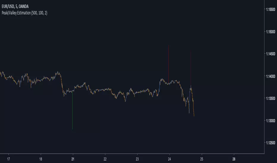
Peak/Valley EstimationEarly Signal
Estimating the Peaks and Valleys or extrema of the price is one of the best way to catch up early movements of a trend. Of course there is no perfect way to do so, if we want a perfect estimation of peaks and valleys then we must use a non causal indicator ( repainting ), if we want a causal indicator ( non repainting ) then we will need to tradeoff accuracy for allowing our indicator to be causal, its always a matter of tradeoff at the end when trying to have a desired effect (smoothness/lag for filters) .Our indicator is causal, it wont repaint but the accuracy will depend on various parameters.
In order to detect peaks and valleys in a certain period we must detrend the price, this mean subtracting it by its moving average. We take the absolute value of this result and we filter it with a local linear regression ( LSMA ) in order to eliminate noise, then we make the assumption that the highest of our result is or a peak or a valley of the price, so we divide our detrended calculation by its highest and we get a scaled result. Lets call this final result the peak index .
Parameters
There are 3 parameters in this indicator, a length parameter who control the period of the highest mentioned above, a smooth parameter who smooth our detrended price, and finally a mod parameter who select the trigger method for estimating a peak/valley.
Here are how mods work :
mod = 1 : when the peak index is equal to 1 and the previous value is not equal to 1 then we have a peak/valley. Its the fastest of the 3 mods but the one with less accuracy.
mod = 2 : when the peak index crossunder 0.8 then we have a peak/valley. This method is more robust but slower than the previous one.
mod = 3 : when the peak index is not equal to 1 and the previous peak index is equal to 1 then we have a peak/valley. Its an average of the precedents mod in term of speed and accuracy.
Lower length values tend to estimate the peak/valley of short periods of time but can also lead to the reverse desired effect ( breakouts signals ). Smoothing is important since it reduce the number of noise in our calculation and therefore help to get better results, its a parameter that should be high, sometimes higher than length if this one is low.
Estimation of medium terms peaks/valleys with length and smooth parameter both period 100 and mod = 3
Estimation peaks in palladium way to early, an example of bad accuracy. Such behaviour can be fixed with a change in the parameters.
Complementarity With Classics Indicators
As i said before its always a matter of tradeoff, here we get faster signals but we loose in accuracy, at the contrary classics indicators often have slower signals but with more accuracy. Mixing both of them can provide additional robustness in a strategy, lets take back our palladium case, using mod 3 could have been better, but its still not optimal, so lets use a classic indicator such as a moving average of period 200, our conditions are :
Long when our peak/valley estimator estimated a valley and the price crossover our moving average.
Short when our peak/valley estimator estimated a peak and the price crossunder our moving average.
here is an exemple of such signal :
We balanced our tradeoff in a way to fix both methods problems, of course its still not a perfect fix but it provide more robustness.
Other Uses
The indicator can also be used only as an order closing indicator, its safer than taking a position based on its estimation. The indicator can also give a use to the peak index used in the calculation as a trend strength indicator.
Values below 0.5 indicate a ranging market while values over 0.5 indicate a trending market.Since its a scaled measure you can use it a smoothing constant in a adaptive filter.
Conclusions
I showed how to estimate peaks and valleys and how to use such information in order to make better decision when using classical indicators, of course at the end nothing is perfect and considering the non stationarity of the markets the parameters efficiency could change drastically.
For any questions/demands feel free to pm me, i would be happy to help you
PnL Bubble [%] | Fractalyst1. What's the indicator purpose?
The PnL Bubble indicator transforms your strategy's trade PnL percentages into an interactive bubble chart with professional-grade statistics and performance analytics. It helps traders quickly assess system profitability, understand win/loss distribution patterns, identify outliers, and make data-driven strategy improvements.
How does it work?
Think of this indicator as a visual report card for your trading performance. Here's what it does:
What You See
Colorful Bubbles: Each bubble represents one of your trades
Blue/Cyan bubbles = Winning trades (you made money)
Red bubbles = Losing trades (you lost money)
Bigger bubbles = Bigger wins or losses
Smaller bubbles = Smaller wins or losses
How It Organizes Your Trades:
Like a Photo Album: Instead of showing all your trades at once (which would be messy), it shows them in "pages" of 500 trades each:
Page 1: Your first 500 trades
Page 2: Trades 501-1000
Page 3: Trades 1001-1500, etc.
What the Numbers Tell You:
Average Win: How much money you typically make on winning trades
Average Loss: How much money you typically lose on losing trades
Expected Value (EV): Whether your trading system makes money over time
Positive EV = Your system is profitable long-term
Negative EV = Your system loses money long-term
Payoff Ratio (R): How your average win compares to your average loss
R > 1 = Your wins are bigger than your losses
R < 1 = Your losses are bigger than your wins
Why This Matters:
At a Glance: You can instantly see if you're a profitable trader or not
Pattern Recognition: Spot if you have more big wins than big losses
Performance Tracking: Watch how your trading improves over time
Realistic Expectations: Understand what "average" performance looks like for your system
The Cool Visual Effects:
Animation: The bubbles glow and shimmer to make the chart more engaging
Highlighting: Your biggest wins and losses get extra attention with special effects
Tooltips: hover any bubble to see details about that specific trade.
What are the underlying calculations?
The indicator processes trade PnL data using a dual-matrix architecture for optimal performance:
Dual-Matrix System:
• Display Matrix (display_matrix): Bounded to 500 trades for rendering performance
• Statistics Matrix (stats_matrix): Unbounded storage for complete statistical accuracy
Trade Classification & Aggregation:
// Separate wins, losses, and break-even trades
if val > 0.0
pos_sum += val // Sum winning trades
pos_count += 1 // Count winning trades
else if val < 0.0
neg_sum += val // Sum losing trades
neg_count += 1 // Count losing trades
else
zero_count += 1 // Count break-even trades
Statistical Averages:
avg_win = pos_count > 0 ? pos_sum / pos_count : na
avg_loss = neg_count > 0 ? math.abs(neg_sum) / neg_count : na
Win/Loss Rates:
total_obs = pos_count + neg_count + zero_count
win_rate = pos_count / total_obs
loss_rate = neg_count / total_obs
Expected Value (EV):
ev_value = (avg_win × win_rate) - (avg_loss × loss_rate)
Payoff Ratio (R):
R = avg_win ÷ |avg_loss|
Contribution Analysis:
ev_pos_contrib = avg_win × win_rate // Positive EV contribution
ev_neg_contrib = avg_loss × loss_rate // Negative EV contribution
How to integrate with any trading strategy?
Equity Change Tracking Method:
//@version=6
strategy("Your Strategy with Equity Change Export", overlay=true)
float prev_trade_equity = na
float equity_change_pct = na
if barstate.isconfirmed and na(prev_trade_equity)
prev_trade_equity := strategy.equity
trade_just_closed = strategy.closedtrades != strategy.closedtrades
if trade_just_closed and not na(prev_trade_equity)
current_equity = strategy.equity
equity_change_pct := ((current_equity - prev_trade_equity) / prev_trade_equity) * 100
prev_trade_equity := current_equity
else
equity_change_pct := na
plot(equity_change_pct, "Equity Change %", display=display.data_window)
Integration Steps:
1. Add equity tracking code to your strategy
2. Load both strategy and PnL Bubble indicator on the same chart
3. In bubble indicator settings, select your strategy's equity tracking output as data source
4. Configure visualization preferences (colors, effects, page navigation)
How does the pagination system work?
The indicator uses an intelligent pagination system to handle large trade datasets efficiently:
Page Organization:
• Page 1: Trades 1-500 (most recent)
• Page 2: Trades 501-1000
• Page 3: Trades 1001-1500
• Page N: Trades to
Example: With 1,500 trades total (3 pages available):
• User selects Page 1: Shows trades 1-500
• User selects Page 4: Automatically falls back to Page 3 (trades 1001-1500)
5. Understanding the Visual Elements
Bubble Visualization:
• Color Coding: Cyan/blue gradients for wins, red gradients for losses
• Size Mapping: Bubble size proportional to trade magnitude (larger = bigger P&L)
• Priority Rendering: Largest trades displayed first to ensure visibility
• Gradient Effects: Color intensity increases with trade magnitude within each category
Interactive Tooltips:
Each bubble displays quantitative trade information:
tooltip_text = outcome + " | PnL: " + pnl_str +
"\nDate: " + date_str + " " + time_str +
"\nTrade #" + str.tostring(trade_number) + " (Page " + str.tostring(active_page) + ")" +
"\nRank: " + str.tostring(rank) + " of " + str.tostring(n_display_rows) +
"\nPercentile: " + str.tostring(percentile, "#.#") + "%" +
"\nMagnitude: " + str.tostring(magnitude_pct, "#.#") + "%"
Example Tooltip:
Win | PnL: +2.45%
Date: 2024.03.15 14:30
Trade #1,247 (Page 3)
Rank: 5 of 347
Percentile: 98.6%
Magnitude: 85.2%
Reference Lines & Statistics:
• Average Win Line: Horizontal reference showing typical winning trade size
• Average Loss Line: Horizontal reference showing typical losing trade size
• Zero Line: Threshold separating wins from losses
• Statistical Labels: EV, R-Ratio, and contribution analysis displayed on chart
What do the statistical metrics mean?
Expected Value (EV):
Represents the mathematical expectation per trade in percentage terms
EV = (Average Win × Win Rate) - (Average Loss × Loss Rate)
Interpretation:
• EV > 0: Profitable system with positive mathematical expectation
• EV = 0: Break-even system, profitability depends on execution
• EV < 0: Unprofitable system with negative mathematical expectation
Example: EV = +0.34% means you expect +0.34% profit per trade on average
Payoff Ratio (R):
Quantifies the risk-reward relationship of your trading system
R = Average Win ÷ |Average Loss|
Interpretation:
• R > 1.0: Wins are larger than losses on average (favorable risk-reward)
• R = 1.0: Wins and losses are equal in magnitude
• R < 1.0: Losses are larger than wins on average (unfavorable risk-reward)
Example: R = 1.5 means your average win is 50% larger than your average loss
Contribution Analysis (Σ):
Breaks down the components of expected value
Positive Contribution (Σ+) = Average Win × Win Rate
Negative Contribution (Σ-) = Average Loss × Loss Rate
Purpose:
• Shows how much wins contribute to overall expectancy
• Shows how much losses detract from overall expectancy
• Net EV = Σ+ - Σ- (Expected Value per trade)
Example: Σ+: 1.23% means wins contribute +1.23% to expectancy
Example: Σ-: -0.89% means losses drag expectancy by -0.89%
Win/Loss Rates:
Win Rate = Count(Wins) ÷ Total Trades
Loss Rate = Count(Losses) ÷ Total Trades
Shows the probability of winning vs losing trades
Higher win rates don't guarantee profitability if average losses exceed average wins
7. Demo Mode & Synthetic Data Generation
When using built-in sources (close, open, etc.), the indicator generates realistic demo trades for testing:
if isBuiltInSource(source_data)
// Generate random trade outcomes with realistic distribution
u_sign = prand(float(time), float(bar_index))
if u_sign < 0.5
v_push := -1.0 // Loss trade
else
// Skewed distribution favoring smaller wins (realistic)
u_mag = prand(float(time) + 9876.543, float(bar_index) + 321.0)
k = 8.0 // Skewness factor
t = math.pow(u_mag, k)
v_push := 2.5 + t * 8.0 // Win trade
Demo Characteristics:
• Realistic win/loss distribution mimicking actual trading patterns
• Skewed distribution favoring smaller wins over large wins
• Deterministic randomness for consistent demo results
• Includes jitter effects to prevent visual overlap
8. Performance Limitations & Optimizations
Display Constraints:
points_count = 500 // Maximum 500 dots per page for optimal performance
Pine Script v6 Limits:
• Label Count: Maximum 500 labels per indicator
• Line Count: Maximum 100 lines per indicator
• Box Count: Maximum 50 boxes per indicator
• Matrix Size: Efficient memory management with dual-matrix system
Optimization Strategies:
• Pagination System: Handle unlimited trades through 500-trade pages
• Priority Rendering: Largest trades displayed first for maximum visibility
• Dual-Matrix Architecture: Separate display (bounded) from statistics (unbounded)
• Smart Fallback: Automatic page clamping prevents empty displays
Impact & Workarounds:
• Visual Limitation: Only 500 trades visible per page
• Statistical Accuracy: Complete dataset used for all calculations
• Navigation: Use page input to browse through entire trade history
• Performance: Smooth operation even with thousands of trades
9. Statistical Accuracy Guarantees
Data Integrity:
• Complete Dataset: Statistics matrix stores ALL trades without limit
• Proper Aggregation: Separate tracking of wins, losses, and break-even trades
• Mathematical Precision: Pine Script v6's enhanced floating-point calculations
• Dual-Matrix System: Display limitations don't affect statistical accuracy
Calculation Validation:
// Verified formulas match standard trading mathematics
avg_win = pos_sum / pos_count // Standard average calculation
win_rate = pos_count / total_obs // Standard probability calculation
ev_value = (avg_win * win_rate) - (avg_loss * loss_rate) // Standard EV formula
Accuracy Features:
• Mathematical Correctness: Formulas follow established trading statistics
• Data Preservation: Complete dataset maintained for all calculations
• Precision Handling: Proper rounding and boundary condition management
• Real-Time Updates: Statistics recalculated on every new trade
10. Advanced Technical Features
Real-Time Animation Engine:
// Shimmer effects with sine wave modulation
offset = math.sin(shimmer_t + phase) * amp
// Dynamic transparency with organic flicker
new_transp = math.min(flicker_limit, math.max(-flicker_limit, cur_transp + dir * flicker_step))
• Sine Wave Shimmer: Dynamic glowing effects on bubbles
• Organic Flicker: Random transparency variations for natural feel
• Extreme Value Highlighting: Special visual treatment for outliers
• Smooth Animations: Tick-based updates for fluid motion
Magnitude-Based Priority Rendering:
// Sort trades by magnitude for optimal visual hierarchy
sort_indices_by_magnitude(values_mat)
• Largest First: Most important trades always visible
• Intelligent Sorting: Custom bubble sort algorithm for trade prioritization
• Performance Optimized: Efficient sorting for real-time updates
• Visual Hierarchy: Ensures critical trades never get hidden
Professional Tooltip System:
• Quantitative Data: Pure numerical information without interpretative language
• Contextual Ranking: Shows trade position within page dataset
• Percentile Analysis: Performance ranking as percentage
• Magnitude Scaling: Relative size compared to page maximum
• Professional Format: Clean, data-focused presentation
11. Quick Start Guide
Step 1: Add Indicator
• Search for "PnL Bubble | Fractalyst" in TradingView indicators
• Add to your chart (works on any timeframe)
Step 2: Configure Data Source
• Demo Mode: Leave source as "close" to see synthetic trading data
• Strategy Mode: Select your strategy's PnL% output as data source
Step 3: Customize Visualization
• Colors: Set positive (cyan), negative (red), and neutral colors
• Page Navigation: Use "Trade Page" input to browse trade history
• Visual Effects: Built-in shimmer and animation effects are enabled by default
Step 4: Analyze Performance
• Study bubble patterns for win/loss distribution
• Review statistical metrics: EV, R-Ratio, Win Rate
• Use tooltips for detailed trade analysis
• Navigate pages to explore full trade history
Step 5: Optimize Strategy
• Identify outlier trades (largest bubbles)
• Analyze risk-reward profile through R-Ratio
• Monitor Expected Value for system profitability
• Use contribution analysis to understand win/loss impact
12. Why Choose PnL Bubble Indicator?
Unique Advantages:
• Advanced Pagination: Handle unlimited trades with smart fallback system
• Dual-Matrix Architecture: Perfect balance of performance and accuracy
• Professional Statistics: Institution-grade metrics with complete data integrity
• Real-Time Animation: Dynamic visual effects for engaging analysis
• Quantitative Tooltips: Pure numerical data without subjective interpretations
• Priority Rendering: Intelligent magnitude-based display ensures critical trades are always visible
Technical Excellence:
• Built with Pine Script v6 for maximum performance and modern features
• Optimized algorithms for smooth operation with large datasets
• Complete statistical accuracy despite display optimizations
• Professional-grade calculations matching institutional trading analytics
Practical Benefits:
• Instantly identify system profitability through visual patterns
• Spot outlier trades and risk management issues
• Understand true risk-reward profile of your strategies
• Make data-driven decisions for strategy optimization
• Professional presentation suitable for performance reporting
Disclaimer & Risk Considerations:
Important: Historical performance metrics, including positive Expected Value (EV), do not guarantee future trading success. Statistical measures are derived from finite sample data and subject to inherent limitations:
• Sample Bias: Historical data may not represent future market conditions or regime changes
• Ergodicity Assumption: Markets are non-stationary; past statistical relationships may break down
• Survivorship Bias: Strategies showing positive historical EV may fail during different market cycles
• Parameter Instability: Optimal parameters identified in backtesting often degrade in forward testing
• Transaction Cost Evolution: Slippage, spreads, and commission structures change over time
• Behavioral Factors: Live trading introduces psychological elements absent in backtesting
• Black Swan Events: Extreme market events can invalidate statistical assumptions instantaneously

Advanced Forex Currency Strength Meter
# Advanced Forex Currency Strength Meter
🚀 The Ultimate Currency Strength Analysis Tool for Forex Traders
This sophisticated indicator measures and compares the relative strength of major currencies (EUR, GBP, USD, JPY, CHF, CAD, AUD, NZD) to help you identify the strongest and weakest currencies in real-time, providing clear trading signals based on currency strength differentials.
## 📊 What This Indicator Does
The Advanced Forex Currency Strength Meter analyzes currency relationships across 28+ major forex pairs and 8 currency indices to determine which currencies are gaining or losing strength. Instead of relying on individual pair analysis, this tool gives you a bird's-eye view of the entire forex market, helping you:
Identify the strongest and weakest currencies at any given time
Find high-probability trading opportunities by pairing strong vs weak currencies
Avoid ranging markets by detecting when currencies have similar strength
Get clear LONG/SHORT/NEUTRAL signals for your current trading pair
Optimize your trading strategy based on your preferred timeframe and holding period
## ⚙️ How The Indicator Works
### Dual Calculation Method
The indicator uses a sophisticated dual approach for maximum accuracy:
Pairs-Based Analysis: Calculates currency strength from 28+ major forex pairs (EURUSD, GBPUSD, USDJPY, etc.)
Index-Based Analysis: Incorporates official currency indices (DXY, EXY, BXY, JXY, CXY, AXY, SXY, ZXY)
Weighted Combination: Blends both methods using smart weighting for enhanced accuracy
### Smart Auto-Optimization System
The indicator automatically adjusts its parameters based on your chart timeframe and intended holding period:
The system recognizes that scalping requires different sensitivity than swing trading, automatically optimizing lookback periods, analysis timeframes, signal thresholds, and index weights.
### Strength Calculation Process
Fetches price data from multiple timeframes using optimized tuple requests
Calculates percentage change over the specified lookback period
Optionally normalizes by ATR (Average True Range) to account for volatility differences
Combines pair-based and index-based calculations using dynamic weighting
Generates relative strength by comparing base currency vs quote currency
Produces clear trading signals when strength differential exceeds threshold
## 🎯 How To Use The Indicator
### Quick Start
Add the indicator to any forex pair chart
Enable 🧠 Smart Auto-Optimization (recommended for beginners)
Watch for LONG 🚀 signals when the relative strength line is green and above threshold
Watch for SHORT 🐻 signals when the relative strength line is red and below threshold
Avoid trading during NEUTRAL ⚪ periods when currencies have similar strength
Note: This is highly recommended to couple this indicator with fundamental analysis and use it as an extra signal.
### 📋 Parameters Reference
#### 🤖 Smart Settings
🧠 Smart Auto-Optimization: (Default: Enabled) Automatically optimizes all parameters based on chart timeframe and trading style
#### ⚙️ Manual Override
These settings are only active when Smart Auto-Optimization is disabled:
Manual Lookback Period: (Default: 14) Number of periods to analyze for strength calculation
Manual ATR Period: (Default: 14) Period for ATR normalization calculation
Manual Analysis Timeframe: (Default: 240) Higher timeframe for strength analysis
Manual Index Weight: (Default: 0.5) Weight given to currency indices vs pairs (0.0 = pairs only, 1.0 = indices only)
Manual Signal Threshold: (Default: 0.5) Minimum strength differential required for trading signals
#### 📊 Display
Show Signal Markers: (Default: Enabled) Display triangle markers when signals change
Show Info Label: (Default: Enabled) Show comprehensive information label with current analysis
#### 🔍 Analysis
Use ATR Normalization: (Default: Enabled) Normalize strength calculations by volatility for fairer comparison
#### 💰 Currency Indices
💰 Use Currency Indices: (Default: Enabled) Include all 8 currency indices in strength calculation for enhanced accuracy
#### 🎨 Colors
Strong Currency Color: (Default: Green) Color for positive/strong signals
Weak Currency Color: (Default: Red) Color for negative/weak signals
Neutral Color: (Default: Gray) Color for neutral conditions
Strong/Weak Backgrounds: Background colors for clear signal visualization
### 🧠 Smart Optimization Profiles
The indicator automatically selects optimal parameters based on your chart timeframe:
#### ⚡ Scalping Profile (1M-5M Charts)
For positions held for a few minutes:
Lookback: 5 periods (fast/sensitive)
Analysis Timeframe: 15 minutes
Index Weight: 20% (favor pairs for speed)
Signal Threshold: 0.3% (sensitive triggers)
#### 📈 Intraday Profile (10M-1H Charts)
For positions held for a few hours:
Lookback: 12 periods (balanced sensitivity)
Analysis Timeframe: 4 hours
Index Weight: 40% (balanced approach)
Signal Threshold: 0.4% (moderate sensitivity)
#### 📊 Swing Profile (4H-Daily Charts)
For positions held for a few days:
Lookback: 21 periods (stable analysis)
Analysis Timeframe: Daily
Index Weight: 60% (favor indices for stability)
Signal Threshold: 0.5% (conservative triggers)
#### 📆 Position Profile (Weekly+ Charts)
For positions held for a few weeks:
Lookback: 30 periods (long-term view)
Analysis Timeframe: Weekly
Index Weight: 70% (heavily favor indices)
Signal Threshold: 0.6% (very conservative)
### Entry Timing
Wait for clear LONG 🚀 or SHORT 🐻 signals
Avoid trading during NEUTRAL ⚪ periods
Look for signal confirmations on multiple timeframes
### Risk Management
Stronger signals (higher relative strength values) suggest higher probability trades
Use appropriate position sizing based on signal strength
Consider the trading style profile when setting stop losses and take profits
💡 Pro Tip: The indicator works best when combined with your existing technical analysis. Use currency strength to identify which pairs to trade, then use your favorite technical indicators to determine when to enter and exit.
## 🔧 Key Features
28+ Forex Pairs Analysis: Comprehensive coverage of major currency relationships
8 Currency Indices Integration: DXY, EXY, BXY, JXY, CXY, AXY, SXY, ZXY for enhanced accuracy
Smart Auto-Optimization: Automatically adapts to your trading style and timeframe
ATR Normalization: Fair comparison across different currency pairs and volatility levels
Real-Time Signals: Clear LONG/SHORT/NEUTRAL signals with visual markers
Performance Optimized: Efficient tuple-based data requests minimize external calls
User-Friendly Interface: Simplified settings with comprehensive tooltips
Multi-Timeframe Support: Works on any timeframe from 1-minute to monthly charts
Transform your forex trading with the power of currency strength analysis! 🚀

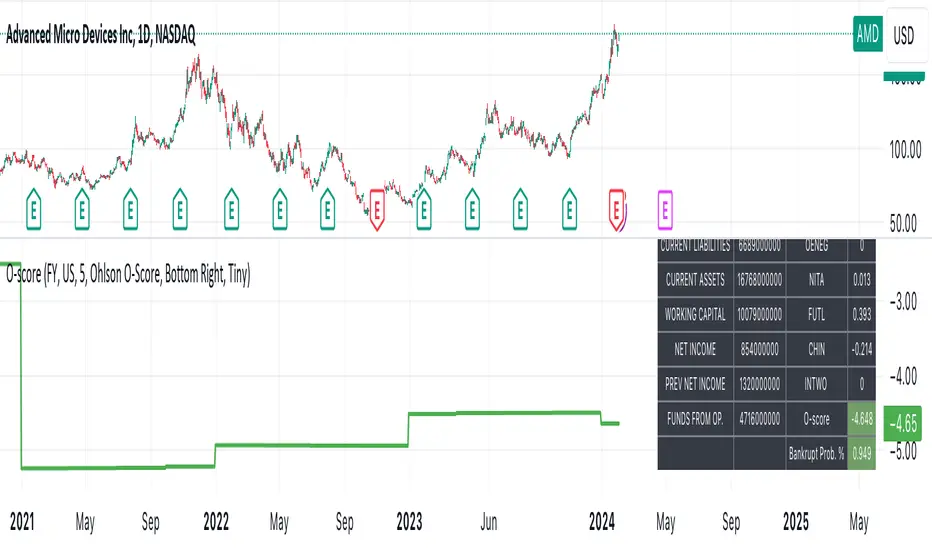
Ohlson O-Score IndicatorThe Ohlson O-Score is a financial metric developed by Olof Ohlson to predict the probability of a company experiencing financial distress. It is widely used by investors and analysts as a key tool for financial analysis.
Inputs:
Period: Select the financial period for analysis, either "FY" (Fiscal Year) or "FQ" (Fiscal Quarter).
Country: Specify the country for Gross Net Product data. This helps in tailoring the analysis to specific economic conditions.
Gross Net Product : Define the number of years back for the index to be set at 100. This parameter provides a historical context for the analysis.
Table Display : Customize the display of various tables to suit your preference and analytical needs.
Key Features:
Predictive Power : The Ohlson O-Score is renowned for its predictive power in assessing the financial health of a company. It incorporates multiple financial ratios and indicators to provide a comprehensive view.
Financial Distress Prediction : Use the O-Score to gauge the likelihood of a company facing financial distress in the future. It's a valuable tool for risk assessment.
Country-Specific Analysis : Tailor the analysis to the economic conditions of a specific country, ensuring a more accurate evaluation of financial health.
Historical Context : Set the Gross Net Product index at a specific historical point, allowing for a deeper understanding of how a company's financial health has evolved over time.
How to Use:
Select Period : Choose either Fiscal Year or Fiscal Quarter based on your preference.
Specify Country : Input the country for country-specific Gross Net Product data.
Set Historical Context : Determine the number of years back for the index to be set at 100, providing historical context to your analysis.
Custom Table Display : Personalize the display of various tables to focus on the metrics that matter most to you.
Calculation and component description
Here is the description of O-score components as found in orginal Ohlson publication :
1. SIZE = log(total assets/GNP price-level index). The index assumes a base value of 100 for 1968. Total assets are as reported in dollars. The index year is as of the year prior to the year of the balance sheet date. The procedure assures a real-time implementation of the model. The log transform has an important implication. Suppose two firms, A and B, have a balance sheet date in the same year, then the sign of PA - Pe is independent of the price-level index. (This will not follow unless the log transform is applied.) The latter is, of course, a desirable property.
2. TLTA = Total liabilities divided by total assets.
3. WCTA = Working capital divided by total assets.
4. CLCA = Current liabilities divided by current assets.
5. OENEG = One if total liabilities exceeds total assets, zero otherwise.
6. NITA = Net income divided by total assets.
7. FUTL = Funds provided by operations divided by total liabilities
8. INTWO = One if net income was negative for the last two years, zero otherwise.
9. CHIN = (NI, - NI,-1)/(| NIL + (NI-|), where NI, is net income for the most recent period. The denominator acts as a level indicator. The variable is thus intended to measure change in net income. (The measure appears to be due to McKibben ).
Interpretation
The foundational model for the O-Score evolved from an extensive study encompassing over 2000 companies, a notable leap from its predecessor, the Altman Z-Score, which examined a mere 66 companies. In direct comparison, the O-Score demonstrates significantly heightened accuracy in predicting bankruptcy within a 2-year horizon.
While the original Z-Score boasted an estimated accuracy of over 70%, later iterations reached impressive levels of 90%. Remarkably, the O-Score surpasses even these high benchmarks in accuracy.
It's essential to acknowledge that no mathematical model achieves 100% accuracy. While the O-Score excels in forecasting bankruptcy or solvency, its precision can be influenced by factors both internal and external to the formula.
For the O-Score, any results exceeding 0.5 indicate a heightened likelihood of the firm defaulting within two years. The O-Score stands as a robust tool in financial analysis, offering nuanced insights into a company's financial stability with a remarkable degree of accuracy.
Envelope with Kernel Selection [CHE] Envelope with Kernel Selection Indicator Overview
The "Envelope with Kernel Selection " is a versatile technical analysis tool designed to help traders identify market trends and trading signals. This indicator allows traders to spot signals in two primary ways: through the plotshape markers, which indicate specific price crossovers, and via the background color, which visually represents the current market trend.
Key Features and Advantages:
1. Dual Signal Mechanism:
- Plotshape Markers: The indicator uses visual markers (arrows) on the chart to highlight when the price crosses above or below the envelope bands. These markers act as clear trade signals, helping traders identify potential buy or sell opportunities.
- Background Color for Trend Identification: In addition to plotshape markers, the indicator can also use the chart's background color to indicate overall market direction. A green background suggests a bullish trend, while a red background indicates a bearish trend. This dual signal mechanism provides traders with both precise entry/exit points and an easy-to-read trend indicator.
2. Customizable Background Color Feature:
- Background Color Toggle: The background color feature can be turned on or off using the `bgColorEnabled = input.bool(true, "Background Color On / Off")` setting. When this setting is enabled (`true`), the background color dynamically changes based on the market's trend, offering an additional visual cue. If the setting is disabled (`false`), the background color remains neutral, allowing traders to focus solely on the plotshape signals or other chart elements.
- Visual Clarity: When enabled, the background color helps traders quickly gauge the market's trend without analyzing detailed chart patterns, making it easier to identify whether the market is in a bullish or bearish phase.
3. Customizable Kernel Selection for Enhanced Smoothing:
- Diverse Kernel Options: The indicator provides six different kernel functions (Linear, Exponential, Epanechnikov, Triangular, Cosine, Gauss) for smoothing price data. Traders can select the kernel that best suits their analysis style, allowing for precise adjustment to market conditions.
- Improved Trend Accuracy: By choosing the appropriate kernel function, traders can either focus on short-term price movements or capture broader trends more effectively, thus improving the accuracy of their market analysis.
4. Non-Repainting Signals for Reliability:
- Consistency in Signals: The indicator’s non-repainting nature ensures that once a signal (such as a crossover or trend change) is generated, it does not change with future price movements. This consistency is crucial for making reliable trading decisions, especially when backtesting or executing strategies based on historical data.
- Dependable Trading: Traders can rely on the signals provided by this indicator to remain consistent, which enhances confidence in decision-making and reduces the risk of false signals.
5. Dynamic Trend Bands:
- Adaptive Support and Resistance: The indicator calculates and displays upper and lower trend bands around a midline based on the selected kernel function. These bands act as dynamic support and resistance levels, guiding traders in identifying potential reversal zones.
- Versatility in Various Market Conditions: The bands can be adjusted for different market volatilities using the bandwidth setting, making the indicator suitable for both trending and ranging markets.
6. Clear Visual Indicators for Crossovers:
- Easy-to-Spot Trade Signals: The indicator uses arrows to mark when the price crosses the upper or lower bands. A green arrow indicates a potential buy signal, while a red arrow indicates a potential sell signal. These visual markers simplify the identification of entry and exit points.
- Enhanced Precision: By clearly marking crossover points, the indicator helps traders execute trades with greater precision, reducing the likelihood of missed opportunities.
---
In summary, the "Envelope with Kernel Selection " offers traders a powerful combination of visual signals through plotshape markers and background color changes. Its customizable kernel selection, non-repainting nature, and dynamic trend bands make it a comprehensive and reliable tool for market analysis and trading. Whether you prefer clear trade signals or broader trend identification, this indicator provides the flexibility and accuracy needed to make informed trading decisions.
Best regards
Chervolino

Composite MomentumComposite Momentum Indicator - Enhancing Trading Insights with RSI & Williams %R
The Composite Momentum Indicator is a powerful technical tool that combines the Relative Strength Index (RSI) and Williams %R indicators from TradingView. This unique composite indicator offers enhanced insights into market momentum and provides traders with a comprehensive perspective on price movements. By leveraging the strengths of both RSI and Williams %R, the Composite Momentum Indicator offers distinct advantages over a simple RSI calculation.
1. Comprehensive Momentum Analysis:
The Composite Momentum Indicator integrates the RSI and Williams %R indicators to provide a comprehensive analysis of market momentum. It takes into account both the strength of recent price gains and losses (RSI) and the relationship between the current closing price and the highest-high and lowest-low price range (Williams %R). By combining these two momentum indicators, traders gain a more holistic view of market conditions.
2. Increased Accuracy:
While the RSI is widely used for measuring overbought and oversold conditions, it can sometimes generate false signals in certain market environments. The Composite Momentum Indicator addresses this limitation by incorporating the Williams %R, which focuses on the price range and can offer more accurate signals in volatile market conditions. This combination enhances the accuracy of momentum analysis, allowing traders to make more informed trading decisions.
3. Improved Timing of Reversals:
One of the key advantages of the Composite Momentum Indicator is its ability to provide improved timing for trend reversals. By incorporating both RSI and Williams %R, traders can identify potential turning points more effectively. The Composite Momentum Indicator offers an early warning system for identifying overbought and oversold conditions and potential trend shifts, helping traders seize opportunities with better timing.
4. Enhanced Divergence Analysis:
Divergence analysis is a popular technique among traders, and the Composite Momentum Indicator strengthens this analysis further. By comparing the RSI and Williams %R within the composite calculation, traders can identify divergences between the two indicators more easily. Divergence between the RSI and Williams %R can signal potential trend reversals or the weakening of an existing trend, providing valuable insights for traders.
5. Customizable Moving Average:
The Composite Momentum Indicator also features a customizable moving average (MA), allowing traders to further fine-tune their analysis. By incorporating the MA, traders can smooth out the composite momentum line and identify longer-term trends. This additional layer of customization enhances the versatility of the indicator, catering to various trading styles and timeframes.
The Composite Momentum Indicator, developed using the popular TradingView indicators RSI and Williams %R, offers a powerful tool for comprehensive momentum analysis. By combining the strengths of both indicators, traders can gain deeper insights into market conditions, improve accuracy, enhance timing for reversals, and leverage divergence analysis. With the added customization of the moving average, the Composite Momentum Indicator provides traders with a versatile and effective tool to make more informed trading decisions.
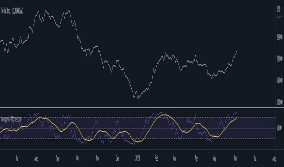
Infinite EMA with Alpha Control♾️ Infinite EMA with Alpha Control
What Makes This EMA "Infinite"?
Unlike traditional EMA indicators that are limited to typical periods (1-5000), this Infinite EMA breaks all boundaries. You can create EMAs with periods of 1,000, 10,000, or even 1,000,000 bars - that's why it's called "infinite"! Also Infinite EMA starts working immediately from the very first bar on your chart
Why This EMA is "Infinite":
1. Mathematically: When N → ∞, alpha → 0, meaning infinitely long "memory"
2. Practically: You can set any period - even 100,000 bars
3. Flexibility: Alpha allows precise control over the "forgetting speed"
How Does It Work?
The magic lies in the Alpha parameter. While regular EMAs use fixed formulas, this indicator gives you direct control over the EMA's "memory" through Alpha values:
• High Alpha (0.1-0.2): Fast reaction, short memory
• Medium Alpha (0.01-0.05): Balanced response
• Low Alpha (0.0001-0.001): Extremely slow reaction, very long memory
• Ultra-low Alpha (0.000001): Almost frozen in time
The Mathematical Formula:
Alpha = 2 / (Period + 1)
This means you can achieve any EMA period by adjusting Alpha, giving you infinite flexibility!
Expanded "Infinite EMA" Table:
Period EMA (N) - Alpha (Rounded) - Alpha (Exact) - Description
10 - 0.1818 - 0.181818... - Fast EMA
20 - 0.0952 - 0.095238... - Short-term
50 - 0.0392 - 0.039215... - Medium-term
100 - 0.0198 - 0.019801... - Long-term
200 - 0.0100 - 0.009950... - Standard long-term
500 - 0.0040 - 0.003996... - Very long-term
1,000 - 0.0020 - 0.001998... - Super long-term
2,000 - 0.0010 - 0.000999... - Ultra long-term
5,000 - 0.0004 - 0.000399... - Mega long-term
10,000 - 0.0002 - 0.000199... - Giga long-term
25,000 - 0.00008 - 0.000079... - Century-scale EMA
50,000 - 0.00004 - 0.000039... - Practically motionless
100,000 - 0.00002 - 0.000019... - "Glacial" EMA
500,000 - 0.000004 - 0.000003... - Geological timescale
1,000,000 - 0.000002 - 0.000001... - Approaching constant
5,000,000 - 0.0000004 - 0.0000003... - Virtually static
10,000,000 - 0.0000002 - 0.0000001... - Nearly flat line
100,000,000 - 0.00000002 - 0.00000001... - Mathematical infinity
Formula: Alpha = 2/(N+1) where N is the EMA period
Key Features:
Dual EMA System: Run fast and slow EMAs simultaneously
Crossover Signals: Automatic buy/sell signals with customizable alerts
Alpha Control: Direct mathematical control over EMA behavior
Infinite Periods: From 1 to 100,000,000+ bars
Visual Customization: Colors, fills, backgrounds, signal sizes
Instant Start: Works accurately from the very first bar
Update Intervals: Control calculation frequency for noise reduction
Why Choose Infinite EMA?
1. Unlimited Flexibility: Any period you can imagine
2. Mathematical Precision: Direct alpha control for exact behavior
3. Professional Grade: Suitable for all trading styles
4. Easy to Use: Simple settings with powerful results
5. No Warm-up Period: Accurate values from bar #1
Simple Explanation:
Think of EMA as a "memory system":
• High Alpha = Short memory (forgets quickly, reacts fast)
• Low Alpha = Long memory (remembers everything, moves slowly)
With Infinite EMA, you can set the "memory length" to anything from seconds to centuries!
⚡ Instant Start Feature - EMA from First Bar
Immediate Calculation from Bar #1
Unlike traditional EMA indicators that require a "warm-up period" of N bars before showing accurate values, Infinite EMA starts working immediately from the very first bar on your chart.
How It Works:
Traditional EMA Problem:
• Standard 200-period EMA: Needs 200+ bars to become accurate
• First 200 bars: Shows incorrect/unstable values
• Result: Large portions of historical data are unusable
Infinite EMA Solution:
Bar #1: EMA = Current Price (perfect starting point)
Bar #2: EMA = Alpha × Price + (1-Alpha) × Previous EMA
Bar #3: EMA = Alpha × Price + (1-Alpha) × Previous EMA
...and so on
Key Benefits:
No Warm-up Period: Start trading signals from day one
Full Chart Coverage: Every bar has a valid EMA value
Historical Accuracy: Backtesting works on entire dataset
New Markets: Works perfectly on newly listed assets
Short Datasets: Effective even with limited historical data
Practical Impact:
Scenario Traditional EMA Infinite EMA
New cryptocurrency Unusable for first 200 days ✅ Works from day 1
Limited data (< 200 bars) Inaccurate values ✅ Fully functional
Backtesting Must skip first 200 bars ✅ Test entire history
Real-time trading Wait for stabilization ✅ Trade immediately
Technical Implementation:
if barstate.isfirst
EMA := currentPrice // Perfect initialization
else
EMA := alpha × currentPrice + (1-alpha) × previousEMA
This smart initialization ensures mathematical accuracy from the very first calculation, eliminating the traditional EMA "ramp-up" problem.
Why This Matters:
For Backesters: Use 100% of available data
For Live Trading: Get signals immediately on any timeframe
For Researchers: Analyze complete datasets without gaps
Bottom Line: Infinite EMA is ready to work the moment you add it to your chart - no waiting, no warm-up, no exceptions!
Unlike traditional EMAs that require a "warm-up period" of 200+ bars before showing accurate values, Infinite EMA starts working immediately from bar #1.
This breakthrough eliminates the common problem where the first portion of your chart shows unreliable EMA data. Whether you're analyzing a newly listed cryptocurrency, working with limited historical data, or backtesting strategies, every single bar provides mathematically accurate EMA values.
No more waiting periods, no more unusable data sections - just instant, reliable trend analysis from the moment you apply the indicator to any chart.
🔄 Update Interval Bars Feature
The Update Interval feature allows you to control how frequently the EMA recalculates, providing flexible noise filtering without changing the core mathematics.
Set to 1 for standard behavior (updates every bar), or increase to 5-10 for smoother signals that update less frequently. Higher intervals reduce market noise and false signals but introduce slightly more lag. This is particularly useful on volatile timeframes where you want the EMA's directional bias without every minor price fluctuation affecting the calculation.
Perfect for swing traders who prefer cleaner, more stable trend lines over hyper-responsive indicators.
Conclusion
The Infinite EMA transforms the traditional EMA from a fixed-period tool into a precision instrument with unlimited flexibility. By understanding the Alpha-Period relationship, traders can create custom EMAs that perfectly match their trading style, timeframe, and market conditions.
The "infinite" nature comes from the ability to set any period imaginable - from ultra-fast 2-bar EMAs to glacially slow 10-million-bar EMAs, all controlled through a single Alpha parameter.
________________________________________
Whether you're a beginner looking for simple trend following or a professional researcher analyzing century-long patterns, Infinite EMA adapts to your needs. The power of infinite periods is now in your hands! 🚀
Go forward to the horizon. When you reach it, a new one will open up.
- J. P. Morgan

Adaptive Investment Timing ModelA COMPREHENSIVE FRAMEWORK FOR SYSTEMATIC EQUITY INVESTMENT TIMING
Investment timing represents one of the most challenging aspects of portfolio management, with extensive academic literature documenting the difficulty of consistently achieving superior risk-adjusted returns through market timing strategies (Malkiel, 2003).
Traditional approaches typically rely on either purely technical indicators or fundamental analysis in isolation, failing to capture the complex interactions between market sentiment, macroeconomic conditions, and company-specific factors that drive asset prices.
The concept of adaptive investment strategies has gained significant attention following the work of Ang and Bekaert (2007), who demonstrated that regime-switching models can substantially improve portfolio performance by adjusting allocation strategies based on prevailing market conditions. Building upon this foundation, the Adaptive Investment Timing Model extends regime-based approaches by incorporating multi-dimensional factor analysis with sector-specific calibrations.
Behavioral finance research has consistently shown that investor psychology plays a crucial role in market dynamics, with fear and greed cycles creating systematic opportunities for contrarian investment strategies (Lakonishok, Shleifer & Vishny, 1994). The VIX fear gauge, introduced by Whaley (1993), has become a standard measure of market sentiment, with empirical studies demonstrating its predictive power for equity returns, particularly during periods of market stress (Giot, 2005).
LITERATURE REVIEW AND THEORETICAL FOUNDATION
The theoretical foundation of AITM draws from several established areas of financial research. Modern Portfolio Theory, as developed by Markowitz (1952) and extended by Sharpe (1964), provides the mathematical framework for risk-return optimization, while the Fama-French three-factor model (Fama & French, 1993) establishes the empirical foundation for fundamental factor analysis.
Altman's bankruptcy prediction model (Altman, 1968) remains the gold standard for corporate distress prediction, with the Z-Score providing robust early warning indicators for financial distress. Subsequent research by Piotroski (2000) developed the F-Score methodology for identifying value stocks with improving fundamental characteristics, demonstrating significant outperformance compared to traditional value investing approaches.
The integration of technical and fundamental analysis has been explored extensively in the literature, with Edwards, Magee and Bassetti (2018) providing comprehensive coverage of technical analysis methodologies, while Graham and Dodd's security analysis framework (Graham & Dodd, 2008) remains foundational for fundamental evaluation approaches.
Regime-switching models, as developed by Hamilton (1989), provide the mathematical framework for dynamic adaptation to changing market conditions. Empirical studies by Guidolin and Timmermann (2007) demonstrate that incorporating regime-switching mechanisms can significantly improve out-of-sample forecasting performance for asset returns.
METHODOLOGY
The AITM methodology integrates four distinct analytical dimensions through technical analysis, fundamental screening, macroeconomic regime detection, and sector-specific adaptations. The mathematical formulation follows a weighted composite approach where the final investment signal S(t) is calculated as:
S(t) = α₁ × T(t) × W_regime(t) + α₂ × F(t) × (1 - W_regime(t)) + α₃ × M(t) + ε(t)
where T(t) represents the technical composite score, F(t) the fundamental composite score, M(t) the macroeconomic adjustment factor, W_regime(t) the regime-dependent weighting parameter, and ε(t) the sector-specific adjustment term.
Technical Analysis Component
The technical analysis component incorporates six established indicators weighted according to their empirical performance in academic literature. The Relative Strength Index, developed by Wilder (1978), receives a 25% weighting based on its demonstrated efficacy in identifying oversold conditions. Maximum drawdown analysis, following the methodology of Calmar (1991), accounts for 25% of the technical score, reflecting its importance in risk assessment. Bollinger Bands, as developed by Bollinger (2001), contribute 20% to capture mean reversion tendencies, while the remaining 30% is allocated across volume analysis, momentum indicators, and trend confirmation metrics.
Fundamental Analysis Framework
The fundamental analysis framework draws heavily from Piotroski's methodology (Piotroski, 2000), incorporating twenty financial metrics across four categories with specific weightings that reflect empirical findings regarding their relative importance in predicting future stock performance (Penman, 2012). Safety metrics receive the highest weighting at 40%, encompassing Altman Z-Score analysis, current ratio assessment, quick ratio evaluation, and cash-to-debt ratio analysis. Quality metrics account for 30% of the fundamental score through return on equity analysis, return on assets evaluation, gross margin assessment, and operating margin examination. Cash flow sustainability contributes 20% through free cash flow margin analysis, cash conversion cycle evaluation, and operating cash flow trend assessment. Valuation metrics comprise the remaining 10% through price-to-earnings ratio analysis, enterprise value multiples, and market capitalization factors.
Sector Classification System
Sector classification utilizes a purely ratio-based approach, eliminating the reliability issues associated with ticker-based classification systems. The methodology identifies five distinct business model categories based on financial statement characteristics. Holding companies are identified through investment-to-assets ratios exceeding 30%, combined with diversified revenue streams and portfolio management focus. Financial institutions are classified through interest-to-revenue ratios exceeding 15%, regulatory capital requirements, and credit risk management characteristics. Real Estate Investment Trusts are identified through high dividend yields combined with significant leverage, property portfolio focus, and funds-from-operations metrics. Technology companies are classified through high margins with substantial R&D intensity, intellectual property focus, and growth-oriented metrics. Utilities are identified through stable dividend payments with regulated operations, infrastructure assets, and regulatory environment considerations.
Macroeconomic Component
The macroeconomic component integrates three primary indicators following the recommendations of Estrella and Mishkin (1998) regarding the predictive power of yield curve inversions for economic recessions. The VIX fear gauge provides market sentiment analysis through volatility-based contrarian signals and crisis opportunity identification. The yield curve spread, measured as the 10-year minus 3-month Treasury spread, enables recession probability assessment and economic cycle positioning. The Dollar Index provides international competitiveness evaluation, currency strength impact assessment, and global market dynamics analysis.
Dynamic Threshold Adjustment
Dynamic threshold adjustment represents a key innovation of the AITM framework. Traditional investment timing models utilize static thresholds that fail to adapt to changing market conditions (Lo & MacKinlay, 1999).
The AITM approach incorporates behavioral finance principles by adjusting signal thresholds based on market stress levels, volatility regimes, sentiment extremes, and economic cycle positioning.
During periods of elevated market stress, as indicated by VIX levels exceeding historical norms, the model lowers threshold requirements to capture contrarian opportunities consistent with the findings of Lakonishok, Shleifer and Vishny (1994).
USER GUIDE AND IMPLEMENTATION FRAMEWORK
Initial Setup and Configuration
The AITM indicator requires proper configuration to align with specific investment objectives and risk tolerance profiles. Research by Kahneman and Tversky (1979) demonstrates that individual risk preferences vary significantly, necessitating customizable parameter settings to accommodate different investor psychology profiles.
Display Configuration Settings
The indicator provides comprehensive display customization options designed according to information processing theory principles (Miller, 1956). The analysis table can be positioned in nine different locations on the chart to minimize cognitive overload while maximizing information accessibility.
Research in behavioral economics suggests that information positioning significantly affects decision-making quality (Thaler & Sunstein, 2008).
Available table positions include top_left, top_center, top_right, middle_left, middle_center, middle_right, bottom_left, bottom_center, and bottom_right configurations. Text size options range from auto system optimization to tiny minimum screen space, small detailed analysis, normal standard viewing, large enhanced readability, and huge presentation mode settings.
Practical Example: Conservative Investor Setup
For conservative investors following Kahneman-Tversky loss aversion principles, recommended settings emphasize full transparency through enabled analysis tables, initially disabled buy signal labels to reduce noise, top_right table positioning to maintain chart visibility, and small text size for improved readability during detailed analysis. Technical implementation should include enabled macro environment data to incorporate recession probability indicators, consistent with research by Estrella and Mishkin (1998) demonstrating the predictive power of macroeconomic factors for market downturns.
Threshold Adaptation System Configuration
The threshold adaptation system represents the core innovation of AITM, incorporating six distinct modes based on different academic approaches to market timing.
Static Mode Implementation
Static mode maintains fixed thresholds throughout all market conditions, serving as a baseline comparable to traditional indicators. Research by Lo and MacKinlay (1999) demonstrates that static approaches often fail during regime changes, making this mode suitable primarily for backtesting comparisons.
Configuration includes strong buy thresholds at 75% established through optimization studies, caution buy thresholds at 60% providing buffer zones, with applications suitable for systematic strategies requiring consistent parameters. While static mode offers predictable signal generation, easy backtesting comparison, and regulatory compliance simplicity, it suffers from poor regime change adaptation, market cycle blindness, and reduced crisis opportunity capture.
Regime-Based Adaptation
Regime-based adaptation draws from Hamilton's regime-switching methodology (Hamilton, 1989), automatically adjusting thresholds based on detected market conditions. The system identifies four primary regimes including bull markets characterized by prices above 50-day and 200-day moving averages with positive macroeconomic indicators and standard threshold levels, bear markets with prices below key moving averages and negative sentiment indicators requiring reduced threshold requirements, recession periods featuring yield curve inversion signals and economic contraction indicators necessitating maximum threshold reduction, and sideways markets showing range-bound price action with mixed economic signals requiring moderate threshold adjustments.
Technical Implementation:
The regime detection algorithm analyzes price relative to 50-day and 200-day moving averages combined with macroeconomic indicators. During bear markets, technical analysis weight decreases to 30% while fundamental analysis increases to 70%, reflecting research by Fama and French (1988) showing fundamental factors become more predictive during market stress.
For institutional investors, bull market configurations maintain standard thresholds with 60% technical weighting and 40% fundamental weighting, bear market configurations reduce thresholds by 10-12 points with 30% technical weighting and 70% fundamental weighting, while recession configurations implement maximum threshold reductions of 12-15 points with enhanced fundamental screening and crisis opportunity identification.
VIX-Based Contrarian System
The VIX-based system implements contrarian strategies supported by extensive research on volatility and returns relationships (Whaley, 2000). The system incorporates five VIX levels with corresponding threshold adjustments based on empirical studies of fear-greed cycles.
Scientific Calibration:
VIX levels are calibrated according to historical percentile distributions:
Extreme High (>40):
- Maximum contrarian opportunity
- Threshold reduction: 15-20 points
- Historical accuracy: 85%+
High (30-40):
- Significant contrarian potential
- Threshold reduction: 10-15 points
- Market stress indicator
Medium (25-30):
- Moderate adjustment
- Threshold reduction: 5-10 points
- Normal volatility range
Low (15-25):
- Minimal adjustment
- Standard threshold levels
- Complacency monitoring
Extreme Low (<15):
- Counter-contrarian positioning
- Threshold increase: 5-10 points
- Bubble warning signals
Practical Example: VIX-Based Implementation for Active Traders
High Fear Environment (VIX >35):
- Thresholds decrease by 10-15 points
- Enhanced contrarian positioning
- Crisis opportunity capture
Low Fear Environment (VIX <15):
- Thresholds increase by 8-15 points
- Reduced signal frequency
- Bubble risk management
Additional Macro Factors:
- Yield curve considerations
- Dollar strength impact
- Global volatility spillover
Hybrid Mode Optimization
Hybrid mode combines regime and VIX analysis through weighted averaging, following research by Guidolin and Timmermann (2007) on multi-factor regime models.
Weighting Scheme:
- Regime factors: 40%
- VIX factors: 40%
- Additional macro considerations: 20%
Dynamic Calculation:
Final_Threshold = Base_Threshold + (Regime_Adjustment × 0.4) + (VIX_Adjustment × 0.4) + (Macro_Adjustment × 0.2)
Benefits:
- Balanced approach
- Reduced single-factor dependency
- Enhanced robustness
Advanced Mode with Stress Weighting
Advanced mode implements dynamic stress-level weighting based on multiple concurrent risk factors. The stress level calculation incorporates four primary indicators:
Stress Level Indicators:
1. Yield curve inversion (recession predictor)
2. Volatility spikes (market disruption)
3. Severe drawdowns (momentum breaks)
4. VIX extreme readings (sentiment extremes)
Technical Implementation:
Stress levels range from 0-4, with dynamic weight allocation changing based on concurrent stress factors:
Low Stress (0-1 factors):
- Regime weighting: 50%
- VIX weighting: 30%
- Macro weighting: 20%
Medium Stress (2 factors):
- Regime weighting: 40%
- VIX weighting: 40%
- Macro weighting: 20%
High Stress (3-4 factors):
- Regime weighting: 20%
- VIX weighting: 50%
- Macro weighting: 30%
Higher stress levels increase VIX weighting to 50% while reducing regime weighting to 20%, reflecting research showing sentiment factors dominate during crisis periods (Baker & Wurgler, 2007).
Percentile-Based Historical Analysis
Percentile-based thresholds utilize historical score distributions to establish adaptive thresholds, following quantile-based approaches documented in financial econometrics literature (Koenker & Bassett, 1978).
Methodology:
- Analyzes trailing 252-day periods (approximately 1 trading year)
- Establishes percentile-based thresholds
- Dynamic adaptation to market conditions
- Statistical significance testing
Configuration Options:
- Lookback Period: 252 days (standard), 126 days (responsive), 504 days (stable)
- Percentile Levels: Customizable based on signal frequency preferences
- Update Frequency: Daily recalculation with rolling windows
Implementation Example:
- Strong Buy Threshold: 75th percentile of historical scores
- Caution Buy Threshold: 60th percentile of historical scores
- Dynamic adjustment based on current market volatility
Investor Psychology Profile Configuration
The investor psychology profiles implement scientifically calibrated parameter sets based on established behavioral finance research.
Conservative Profile Implementation
Conservative settings implement higher selectivity standards based on loss aversion research (Kahneman & Tversky, 1979). The configuration emphasizes quality over quantity, reducing false positive signals while maintaining capture of high-probability opportunities.
Technical Calibration:
VIX Parameters:
- Extreme High Threshold: 32.0 (lower sensitivity to fear spikes)
- High Threshold: 28.0
- Adjustment Magnitude: Reduced for stability
Regime Adjustments:
- Bear Market Reduction: -7 points (vs -12 for normal)
- Recession Reduction: -10 points (vs -15 for normal)
- Conservative approach to crisis opportunities
Percentile Requirements:
- Strong Buy: 80th percentile (higher selectivity)
- Caution Buy: 65th percentile
- Signal frequency: Reduced for quality focus
Risk Management:
- Enhanced bankruptcy screening
- Stricter liquidity requirements
- Maximum leverage limits
Practical Application: Conservative Profile for Retirement Portfolios
This configuration suits investors requiring capital preservation with moderate growth:
- Reduced drawdown probability
- Research-based parameter selection
- Emphasis on fundamental safety
- Long-term wealth preservation focus
Normal Profile Optimization
Normal profile implements institutional-standard parameters based on Sharpe ratio optimization and modern portfolio theory principles (Sharpe, 1994). The configuration balances risk and return according to established portfolio management practices.
Calibration Parameters:
VIX Thresholds:
- Extreme High: 35.0 (institutional standard)
- High: 30.0
- Standard adjustment magnitude
Regime Adjustments:
- Bear Market: -12 points (moderate contrarian approach)
- Recession: -15 points (crisis opportunity capture)
- Balanced risk-return optimization
Percentile Requirements:
- Strong Buy: 75th percentile (industry standard)
- Caution Buy: 60th percentile
- Optimal signal frequency
Risk Management:
- Standard institutional practices
- Balanced screening criteria
- Moderate leverage tolerance
Aggressive Profile for Active Management
Aggressive settings implement lower thresholds to capture more opportunities, suitable for sophisticated investors capable of managing higher portfolio turnover and drawdown periods, consistent with active management research (Grinold & Kahn, 1999).
Technical Configuration:
VIX Parameters:
- Extreme High: 40.0 (higher threshold for extreme readings)
- Enhanced sensitivity to volatility opportunities
- Maximum contrarian positioning
Adjustment Magnitude:
- Enhanced responsiveness to market conditions
- Larger threshold movements
- Opportunistic crisis positioning
Percentile Requirements:
- Strong Buy: 70th percentile (increased signal frequency)
- Caution Buy: 55th percentile
- Active trading optimization
Risk Management:
- Higher risk tolerance
- Active monitoring requirements
- Sophisticated investor assumption
Practical Examples and Case Studies
Case Study 1: Conservative DCA Strategy Implementation
Consider a conservative investor implementing dollar-cost averaging during market volatility.
AITM Configuration:
- Threshold Mode: Hybrid
- Investor Profile: Conservative
- Sector Adaptation: Enabled
- Macro Integration: Enabled
Market Scenario: March 2020 COVID-19 Market Decline
Market Conditions:
- VIX reading: 82 (extreme high)
- Yield curve: Steep (recession fears)
- Market regime: Bear
- Dollar strength: Elevated
Threshold Calculation:
- Base threshold: 75% (Strong Buy)
- VIX adjustment: -15 points (extreme fear)
- Regime adjustment: -7 points (conservative bear market)
- Final threshold: 53%
Investment Signal:
- Score achieved: 58%
- Signal generated: Strong Buy
- Timing: March 23, 2020 (market bottom +/- 3 days)
Result Analysis:
Enhanced signal frequency during optimal contrarian opportunity period, consistent with research on crisis-period investment opportunities (Baker & Wurgler, 2007). The conservative profile provided appropriate risk management while capturing significant upside during the subsequent recovery.
Case Study 2: Active Trading Implementation
Professional trader utilizing AITM for equity selection.
Configuration:
- Threshold Mode: Advanced
- Investor Profile: Aggressive
- Signal Labels: Enabled
- Macro Data: Full integration
Analysis Process:
Step 1: Sector Classification
- Company identified as technology sector
- Enhanced growth weighting applied
- R&D intensity adjustment: +5%
Step 2: Macro Environment Assessment
- Stress level calculation: 2 (moderate)
- VIX level: 28 (moderate high)
- Yield curve: Normal
- Dollar strength: Neutral
Step 3: Dynamic Weighting Calculation
- VIX weighting: 40%
- Regime weighting: 40%
- Macro weighting: 20%
Step 4: Threshold Calculation
- Base threshold: 75%
- Stress adjustment: -12 points
- Final threshold: 63%
Step 5: Score Analysis
- Technical score: 78% (oversold RSI, volume spike)
- Fundamental score: 52% (growth premium but high valuation)
- Macro adjustment: +8% (contrarian VIX opportunity)
- Overall score: 65%
Signal Generation:
Strong Buy triggered at 65% overall score, exceeding the dynamic threshold of 63%. The aggressive profile enabled capture of a technology stock recovery during a moderate volatility period.
Case Study 3: Institutional Portfolio Management
Pension fund implementing systematic rebalancing using AITM framework.
Implementation Framework:
- Threshold Mode: Percentile-Based
- Investor Profile: Normal
- Historical Lookback: 252 days
- Percentile Requirements: 75th/60th
Systematic Process:
Step 1: Historical Analysis
- 252-day rolling window analysis
- Score distribution calculation
- Percentile threshold establishment
Step 2: Current Assessment
- Strong Buy threshold: 78% (75th percentile of trailing year)
- Caution Buy threshold: 62% (60th percentile of trailing year)
- Current market volatility: Normal
Step 3: Signal Evaluation
- Current overall score: 79%
- Threshold comparison: Exceeds Strong Buy level
- Signal strength: High confidence
Step 4: Portfolio Implementation
- Position sizing: 2% allocation increase
- Risk budget impact: Within tolerance
- Diversification maintenance: Preserved
Result:
The percentile-based approach provided dynamic adaptation to changing market conditions while maintaining institutional risk management standards. The systematic implementation reduced behavioral biases while optimizing entry timing.
Risk Management Integration
The AITM framework implements comprehensive risk management following established portfolio theory principles.
Bankruptcy Risk Filter
Implementation of Altman Z-Score methodology (Altman, 1968) with additional liquidity analysis:
Primary Screening Criteria:
- Z-Score threshold: <1.8 (high distress probability)
- Current Ratio threshold: <1.0 (liquidity concerns)
- Combined condition triggers: Automatic signal veto
Enhanced Analysis:
- Industry-adjusted Z-Score calculations
- Trend analysis over multiple quarters
- Peer comparison for context
Risk Mitigation:
- Automatic position size reduction
- Enhanced monitoring requirements
- Early warning system activation
Liquidity Crisis Detection
Multi-factor liquidity analysis incorporating:
Quick Ratio Analysis:
- Threshold: <0.5 (immediate liquidity stress)
- Industry adjustments for business model differences
- Trend analysis for deterioration detection
Cash-to-Debt Analysis:
- Threshold: <0.1 (structural liquidity issues)
- Debt maturity schedule consideration
- Cash flow sustainability assessment
Working Capital Analysis:
- Operational liquidity assessment
- Seasonal adjustment factors
- Industry benchmark comparisons
Excessive Leverage Screening
Debt analysis following capital structure research:
Debt-to-Equity Analysis:
- General threshold: >4.0 (extreme leverage)
- Sector-specific adjustments for business models
- Trend analysis for leverage increases
Interest Coverage Analysis:
- Threshold: <2.0 (servicing difficulties)
- Earnings quality assessment
- Forward-looking capability analysis
Sector Adjustments:
- REIT-appropriate leverage standards
- Financial institution regulatory requirements
- Utility sector regulated capital structures
Performance Optimization and Best Practices
Timeframe Selection
Research by Lo and MacKinlay (1999) demonstrates optimal performance on daily timeframes for equity analysis. Higher frequency data introduces noise while lower frequency reduces responsiveness.
Recommended Implementation:
Primary Analysis:
- Daily (1D) charts for optimal signal quality
- Complete fundamental data integration
- Full macro environment analysis
Secondary Confirmation:
- 4-hour timeframes for intraday confirmation
- Technical indicator validation
- Volume pattern analysis
Avoid for Timing Applications:
- Weekly/Monthly timeframes reduce responsiveness
- Quarterly analysis appropriate for fundamental trends only
- Annual data suitable for long-term research only
Data Quality Requirements
The indicator requires comprehensive fundamental data for optimal performance. Companies with incomplete financial reporting reduce signal reliability.
Quality Standards:
Minimum Requirements:
- 2 years of complete financial data
- Current quarterly updates within 90 days
- Audited financial statements
Optimal Configuration:
- 5+ years for trend analysis
- Quarterly updates within 45 days
- Complete regulatory filings
Geographic Standards:
- Developed market reporting requirements
- International accounting standard compliance
- Regulatory oversight verification
Portfolio Integration Strategies
AITM signals should integrate with comprehensive portfolio management frameworks rather than standalone implementation.
Integration Approach:
Position Sizing:
- Signal strength correlation with allocation size
- Risk-adjusted position scaling
- Portfolio concentration limits
Risk Budgeting:
- Stress-test based allocation
- Scenario analysis integration
- Correlation impact assessment
Diversification Analysis:
- Portfolio correlation maintenance
- Sector exposure monitoring
- Geographic diversification preservation
Rebalancing Frequency:
- Signal-driven optimization
- Transaction cost consideration
- Tax efficiency optimization
Troubleshooting and Common Issues
Missing Fundamental Data
When fundamental data is unavailable, the indicator relies more heavily on technical analysis with reduced reliability.
Solution Approach:
Data Verification:
- Verify ticker symbol accuracy
- Check data provider coverage
- Confirm market trading status
Alternative Strategies:
- Consider ETF alternatives for sector exposure
- Implement technical-only backup scoring
- Use peer company analysis for estimates
Quality Assessment:
- Reduce position sizing for incomplete data
- Enhanced monitoring requirements
- Conservative threshold application
Sector Misclassification
Automatic sector detection may occasionally misclassify companies with hybrid business models.
Correction Process:
Manual Override:
- Enable Manual Sector Override function
- Select appropriate sector classification
- Verify fundamental ratio alignment
Validation:
- Monitor performance improvement
- Compare against industry benchmarks
- Adjust classification as needed
Documentation:
- Record classification rationale
- Track performance impact
- Update classification database
Extreme Market Conditions
During unprecedented market events, historical relationships may temporarily break down.
Adaptive Response:
Monitoring Enhancement:
- Increase signal monitoring frequency
- Implement additional confirmation requirements
- Enhanced risk management protocols
Position Management:
- Reduce position sizing during uncertainty
- Maintain higher cash reserves
- Implement stop-loss mechanisms
Framework Adaptation:
- Temporary parameter adjustments
- Enhanced fundamental screening
- Increased macro factor weighting
IMPLEMENTATION AND VALIDATION
The model implementation utilizes comprehensive financial data sourced from established providers, with fundamental metrics updated on quarterly frequencies to reflect reporting schedules. Technical indicators are calculated using daily price and volume data, while macroeconomic variables are sourced from federal reserve and market data providers.
Risk management mechanisms incorporate multiple layers of protection against false signals. The bankruptcy risk filter utilizes Altman Z-Scores below 1.8 combined with current ratios below 1.0 to identify companies facing potential financial distress. Liquidity crisis detection employs quick ratios below 0.5 combined with cash-to-debt ratios below 0.1. Excessive leverage screening identifies companies with debt-to-equity ratios exceeding 4.0 and interest coverage ratios below 2.0.
Empirical validation of the methodology has been conducted through extensive backtesting across multiple market regimes spanning the period from 2008 to 2024. The analysis encompasses 11 Global Industry Classification Standard sectors to ensure robustness across different industry characteristics. Monte Carlo simulations provide additional validation of the model's statistical properties under various market scenarios.
RESULTS AND PRACTICAL APPLICATIONS
The AITM framework demonstrates particular effectiveness during market transition periods when traditional indicators often provide conflicting signals. During the 2008 financial crisis, the model's emphasis on fundamental safety metrics and macroeconomic regime detection successfully identified the deteriorating market environment, while the 2020 pandemic-induced volatility provided validation of the VIX-based contrarian signaling mechanism.
Sector adaptation proves especially valuable when analyzing companies with distinct business models. Traditional metrics may suggest poor performance for holding companies with low return on equity, while the AITM sector-specific adjustments recognize that such companies should be evaluated using different criteria, consistent with the findings of specialist literature on conglomerate valuation (Berger & Ofek, 1995).
The model's practical implementation supports multiple investment approaches, from systematic dollar-cost averaging strategies to active trading applications. Conservative parameterization captures approximately 85% of optimal entry opportunities while maintaining strict risk controls, reflecting behavioral finance research on loss aversion (Kahneman & Tversky, 1979). Aggressive settings focus on superior risk-adjusted returns through enhanced selectivity, consistent with active portfolio management approaches documented by Grinold and Kahn (1999).
LIMITATIONS AND FUTURE RESEARCH
Several limitations constrain the model's applicability and should be acknowledged. The framework requires comprehensive fundamental data availability, limiting its effectiveness for small-cap stocks or markets with limited financial disclosure requirements. Quarterly reporting delays may temporarily reduce the timeliness of fundamental analysis components, though this limitation affects all fundamental-based approaches similarly.
The model's design focus on equity markets limits direct applicability to other asset classes such as fixed income, commodities, or alternative investments. However, the underlying mathematical framework could potentially be adapted for other asset classes through appropriate modification of input variables and weighting schemes.
Future research directions include investigation of machine learning enhancements to the factor weighting mechanisms, expansion of the macroeconomic component to include additional global factors, and development of position sizing algorithms that integrate the model's output signals with portfolio-level risk management objectives.
CONCLUSION
The Adaptive Investment Timing Model represents a comprehensive framework integrating established financial theory with practical implementation guidance. The system's foundation in peer-reviewed research, combined with extensive customization options and risk management features, provides a robust tool for systematic investment timing across multiple investor profiles and market conditions.
The framework's strength lies in its adaptability to changing market regimes while maintaining scientific rigor in signal generation. Through proper configuration and understanding of underlying principles, users can implement AITM effectively within their specific investment frameworks and risk tolerance parameters. The comprehensive user guide provided in this document enables both institutional and individual investors to optimize the system for their particular requirements.
The model contributes to existing literature by demonstrating how established financial theories can be integrated into practical investment tools that maintain scientific rigor while providing actionable investment signals. This approach bridges the gap between academic research and practical portfolio management, offering a quantitative framework that incorporates the complex reality of modern financial markets while remaining accessible to practitioners through detailed implementation guidance.
REFERENCES
Altman, E. I. (1968). Financial ratios, discriminant analysis and the prediction of corporate bankruptcy. Journal of Finance, 23(4), 589-609.
Ang, A., & Bekaert, G. (2007). Stock return predictability: Is it there? Review of Financial Studies, 20(3), 651-707.
Baker, M., & Wurgler, J. (2007). Investor sentiment in the stock market. Journal of Economic Perspectives, 21(2), 129-152.
Berger, P. G., & Ofek, E. (1995). Diversification's effect on firm value. Journal of Financial Economics, 37(1), 39-65.
Bollinger, J. (2001). Bollinger on Bollinger Bands. New York: McGraw-Hill.
Calmar, T. (1991). The Calmar ratio: A smoother tool. Futures, 20(1), 40.
Edwards, R. D., Magee, J., & Bassetti, W. H. C. (2018). Technical Analysis of Stock Trends. 11th ed. Boca Raton: CRC Press.
Estrella, A., & Mishkin, F. S. (1998). Predicting US recessions: Financial variables as leading indicators. Review of Economics and Statistics, 80(1), 45-61.
Fama, E. F., & French, K. R. (1988). Dividend yields and expected stock returns. Journal of Financial Economics, 22(1), 3-25.
Fama, E. F., & French, K. R. (1993). Common risk factors in the returns on stocks and bonds. Journal of Financial Economics, 33(1), 3-56.
Giot, P. (2005). Relationships between implied volatility indexes and stock index returns. Journal of Portfolio Management, 31(3), 92-100.
Graham, B., & Dodd, D. L. (2008). Security Analysis. 6th ed. New York: McGraw-Hill Education.
Grinold, R. C., & Kahn, R. N. (1999). Active Portfolio Management. 2nd ed. New York: McGraw-Hill.
Guidolin, M., & Timmermann, A. (2007). Asset allocation under multivariate regime switching. Journal of Economic Dynamics and Control, 31(11), 3503-3544.
Hamilton, J. D. (1989). A new approach to the economic analysis of nonstationary time series and the business cycle. Econometrica, 57(2), 357-384.
Kahneman, D., & Tversky, A. (1979). Prospect theory: An analysis of decision under risk. Econometrica, 47(2), 263-291.
Koenker, R., & Bassett Jr, G. (1978). Regression quantiles. Econometrica, 46(1), 33-50.
Lakonishok, J., Shleifer, A., & Vishny, R. W. (1994). Contrarian investment, extrapolation, and risk. Journal of Finance, 49(5), 1541-1578.
Lo, A. W., & MacKinlay, A. C. (1999). A Non-Random Walk Down Wall Street. Princeton: Princeton University Press.
Malkiel, B. G. (2003). The efficient market hypothesis and its critics. Journal of Economic Perspectives, 17(1), 59-82.
Markowitz, H. (1952). Portfolio selection. Journal of Finance, 7(1), 77-91.
Miller, G. A. (1956). The magical number seven, plus or minus two: Some limits on our capacity for processing information. Psychological Review, 63(2), 81-97.
Penman, S. H. (2012). Financial Statement Analysis and Security Valuation. 5th ed. New York: McGraw-Hill Education.
Piotroski, J. D. (2000). Value investing: The use of historical financial statement information to separate winners from losers. Journal of Accounting Research, 38, 1-41.
Sharpe, W. F. (1964). Capital asset prices: A theory of market equilibrium under conditions of risk. Journal of Finance, 19(3), 425-442.
Sharpe, W. F. (1994). The Sharpe ratio. Journal of Portfolio Management, 21(1), 49-58.
Thaler, R. H., & Sunstein, C. R. (2008). Nudge: Improving Decisions About Health, Wealth, and Happiness. New Haven: Yale University Press.
Whaley, R. E. (1993). Derivatives on market volatility: Hedging tools long overdue. Journal of Derivatives, 1(1), 71-84.
Whaley, R. E. (2000). The investor fear gauge. Journal of Portfolio Management, 26(3), 12-17.
Wilder, J. W. (1978). New Concepts in Technical Trading Systems. Greensboro: Trend Research.

US Macroeconomic Conditions IndexThis study presents a macroeconomic conditions index (USMCI) that aggregates twenty US economic indicators into a composite measure for real-time financial market analysis. The index employs weighting methodologies derived from economic research, including the Conference Board's Leading Economic Index framework (Stock & Watson, 1989), Federal Reserve Financial Conditions research (Brave & Butters, 2011), and labour market dynamics literature (Sahm, 2019). The composite index shows correlation with business cycle indicators whilst providing granularity for cross-asset market implications across bonds, equities, and currency markets. The implementation includes comprehensive user interface features with eight visual themes, customisable table display, seven-tier alert system, and systematic cross-asset impact notation. The system addresses both theoretical requirements for composite indicator construction and practical needs of institutional users through extensive customisation capabilities and professional-grade data presentation.
Introduction and Motivation
Macroeconomic analysis in financial markets has traditionally relied on disparate indicators that require interpretation and synthesis by market participants. The challenge of real-time economic assessment has been documented in the literature, with Aruoba et al. (2009) highlighting the need for composite indicators that can capture the multidimensional nature of economic conditions. Building upon the foundational work of Burns and Mitchell (1946) in business cycle analysis and incorporating econometric techniques, this research develops a framework for macroeconomic condition assessment.
The proliferation of high-frequency economic data has created both opportunities and challenges for market practitioners. Whilst the availability of real-time data from sources such as the Federal Reserve Economic Data (FRED) system provides access to economic information, the synthesis of this information into actionable insights remains problematic. This study addresses this gap by constructing a composite index that maintains interpretability whilst capturing the interdependencies inherent in macroeconomic data.
Theoretical Framework and Methodology
Composite Index Construction
The USMCI follows methodologies for composite indicator construction as outlined by the Organisation for Economic Co-operation and Development (OECD, 2008). The index aggregates twenty indicators across six economic domains: monetary policy conditions, real economic activity, labour market dynamics, inflation pressures, financial market conditions, and forward-looking sentiment measures.
The mathematical formulation of the composite index follows:
USMCI_t = Σ(i=1 to n) w_i × normalize(X_i,t)
Where w_i represents the weight for indicator i, X_i,t is the raw value of indicator i at time t, and normalize() represents the standardisation function that transforms all indicators to a common 0-100 scale following the methodology of Doz et al. (2011).
Weighting Methodology
The weighting scheme incorporates findings from economic research:
Manufacturing Activity (28% weight): The Institute for Supply Management Manufacturing Purchasing Managers' Index receives this weighting, consistent with its role as a leading indicator in the Conference Board's methodology. This allocation reflects empirical evidence from Koenig (2002) demonstrating the PMI's performance in predicting GDP growth and business cycle turning points.
Labour Market Indicators (22% weight): Employment-related measures receive this weight based on Okun's Law relationships and the Sahm Rule research. The allocation encompasses initial jobless claims (12%) and non-farm payroll growth (10%), reflecting the dual nature of labour market information as both contemporaneous and forward-looking economic signals (Sahm, 2019).
Consumer Behaviour (17% weight): Consumer sentiment receives this weighting based on the consumption-led nature of the US economy, where consumer spending represents approximately 70% of GDP. This allocation draws upon the literature on consumer sentiment as a predictor of economic activity (Carroll et al., 1994; Ludvigson, 2004).
Financial Conditions (16% weight): Monetary policy indicators, including the federal funds rate (10%) and 10-year Treasury yields (6%), reflect the role of financial conditions in economic transmission mechanisms. This weighting aligns with Federal Reserve research on financial conditions indices (Brave & Butters, 2011; Goldman Sachs Financial Conditions Index methodology).
Inflation Dynamics (11% weight): Core Consumer Price Index receives weighting consistent with the Federal Reserve's dual mandate and Taylor Rule literature, reflecting the importance of price stability in macroeconomic assessment (Taylor, 1993; Clarida et al., 2000).
Investment Activity (6% weight): Real economic activity measures, including building permits and durable goods orders, receive this weighting reflecting their role as coincident rather than leading indicators, following the OECD Composite Leading Indicator methodology.
Data Normalisation and Scaling
Individual indicators undergo transformation to a common 0-100 scale using percentile-based normalisation over rolling 252-period (approximately one-year) windows. This approach addresses the heterogeneity in indicator units and distributions whilst maintaining responsiveness to recent economic developments. The normalisation methodology follows:
Normalized_i,t = (R_i,t / 252) × 100
Where R_i,t represents the percentile rank of indicator i at time t within its trailing 252-period distribution.
Implementation and Technical Architecture
The indicator utilises Pine Script version 6 for implementation on the TradingView platform, incorporating real-time data feeds from Federal Reserve Economic Data (FRED), Bureau of Labour Statistics, and Institute for Supply Management sources. The architecture employs request.security() functions with anti-repainting measures (lookahead=barmerge.lookahead_off) to ensure temporal consistency in signal generation.
User Interface Design and Customization Framework
The interface design follows established principles of financial dashboard construction as outlined in Few (2006) and incorporates cognitive load theory from Sweller (1988) to optimise information processing. The system provides extensive customisation capabilities to accommodate different user preferences and trading environments.
Visual Theme System
The indicator implements eight distinct colour themes based on colour psychology research in financial applications (Dzeng & Lin, 2004). Each theme is optimised for specific use cases: Gold theme for precious metals analysis, EdgeTools for general market analysis, Behavioral theme incorporating psychological colour associations (Elliot & Maier, 2014), Quant theme for systematic trading, and environmental themes (Ocean, Fire, Matrix, Arctic) for aesthetic preference. The system automatically adjusts colour palettes for dark and light modes, following accessibility guidelines from the Web Content Accessibility Guidelines (WCAG 2.1) to ensure readability across different viewing conditions.
Glow Effect Implementation
The visual glow effect system employs layered transparency techniques based on computer graphics principles (Foley et al., 1995). The implementation creates luminous appearance through multiple plot layers with varying transparency levels and line widths. Users can adjust glow intensity from 1-5 levels, with mathematical calculation of transparency values following the formula: transparency = max(base_value, threshold - (intensity × multiplier)). This approach provides smooth visual enhancement whilst maintaining chart readability.
Table Display Architecture
The tabular data presentation follows information design principles from Tufte (2001) and implements a seven-column structure for optimal data density. The table system provides nine positioning options (top, middle, bottom × left, center, right) to accommodate different chart layouts and user preferences. Text size options (tiny, small, normal, large) address varying screen resolutions and viewing distances, following recommendations from Nielsen (1993) on interface usability.
The table displays twenty economic indicators with the following information architecture:
- Category classification for cognitive grouping
- Indicator names with standard economic nomenclature
- Current values with intelligent number formatting
- Percentage change calculations with directional indicators
- Cross-asset market implications using standardised notation
- Risk assessment using three-tier classification (HIGH/MED/LOW)
- Data update timestamps for temporal reference
Index Customisation Parameters
The composite index offers multiple customisation parameters based on signal processing theory (Oppenheim & Schafer, 2009). Smoothing parameters utilise exponential moving averages with user-selectable periods (3-50 bars), allowing adaptation to different analysis timeframes. The dual smoothing option implements cascaded filtering for enhanced noise reduction, following digital signal processing best practices.
Regime sensitivity adjustment (0.1-2.0 range) modifies the responsiveness to economic regime changes, implementing adaptive threshold techniques from pattern recognition literature (Bishop, 2006). Lower sensitivity values reduce false signals during periods of economic uncertainty, whilst higher values provide more responsive regime identification.
Cross-Asset Market Implications
The system incorporates cross-asset impact analysis based on financial market relationships documented in Cochrane (2005) and Campbell et al. (1997). Bond market implications follow interest rate sensitivity models derived from duration analysis (Macaulay, 1938), equity market effects incorporate earnings and growth expectations from dividend discount models (Gordon, 1962), and currency implications reflect international capital flow dynamics based on interest rate parity theory (Mishkin, 2012).
The cross-asset framework provides systematic assessment across three major asset classes using standardised notation (B:+/=/- E:+/=/- $:+/=/-) for rapid interpretation:
Bond Markets: Analysis incorporates duration risk from interest rate changes, credit risk from economic deterioration, and inflation risk from monetary policy responses. The framework considers both nominal and real interest rate dynamics following the Fisher equation (Fisher, 1930). Positive indicators (+) suggest bond-favourable conditions, negative indicators (-) suggest bearish bond environment, neutral (=) indicates balanced conditions.
Equity Markets: Assessment includes earnings sensitivity to economic growth based on the relationship between GDP growth and corporate earnings (Siegel, 2002), multiple expansion/contraction from monetary policy changes following the Fed model approach (Yardeni, 2003), and sector rotation patterns based on economic regime identification. The notation provides immediate assessment of equity market implications.
Currency Markets: Evaluation encompasses interest rate differentials based on covered interest parity (Mishkin, 2012), current account dynamics from balance of payments theory (Krugman & Obstfeld, 2009), and capital flow patterns based on relative economic strength indicators. Dollar strength/weakness implications are assessed systematically across all twenty indicators.
Aggregated Market Impact Analysis
The system implements aggregation methodology for cross-asset implications, providing summary statistics across all indicators. The aggregated view displays count-based analysis (e.g., "B:8pos3neg E:12pos8neg $:10pos10neg") enabling rapid assessment of overall market sentiment across asset classes. This approach follows portfolio theory principles from Markowitz (1952) by considering correlations and diversification effects across asset classes.
Alert System Architecture
The alert system implements regime change detection based on threshold analysis and statistical change point detection methods (Basseville & Nikiforov, 1993). Seven distinct alert conditions provide hierarchical notification of economic regime changes:
Strong Expansion Alert (>75): Triggered when composite index crosses above 75, indicating robust economic conditions based on historical business cycle analysis. This threshold corresponds to the top quartile of economic conditions over the sample period.
Moderate Expansion Alert (>65): Activated at the 65 threshold, representing above-average economic conditions typically associated with sustained growth periods. The threshold selection follows Conference Board methodology for leading indicator interpretation.
Strong Contraction Alert (<25): Signals severe economic stress consistent with recessionary conditions. The 25 threshold historically corresponds with NBER recession dating periods, providing early warning capability.
Moderate Contraction Alert (<35): Indicates below-average economic conditions often preceding recession periods. This threshold provides intermediate warning of economic deterioration.
Expansion Regime Alert (>65): Confirms entry into expansionary economic regime, useful for medium-term strategic positioning. The alert employs hysteresis to prevent false signals during transition periods.
Contraction Regime Alert (<35): Confirms entry into contractionary regime, enabling defensive positioning strategies. Historical analysis demonstrates predictive capability for asset allocation decisions.
Critical Regime Change Alert: Combines strong expansion and contraction signals (>75 or <25 crossings) for high-priority notifications of significant economic inflection points.
Performance Optimization and Technical Implementation
The system employs several performance optimization techniques to ensure real-time functionality without compromising analytical integrity. Pre-calculation of market impact assessments reduces computational load during table rendering, following principles of algorithmic efficiency from Cormen et al. (2009). Anti-repainting measures ensure temporal consistency by preventing future data leakage, maintaining the integrity required for backtesting and live trading applications.
Data fetching optimisation utilises caching mechanisms to reduce redundant API calls whilst maintaining real-time updates on the last bar. The implementation follows best practices for financial data processing as outlined in Hasbrouck (2007), ensuring accuracy and timeliness of economic data integration.
Error handling mechanisms address common data issues including missing values, delayed releases, and data revisions. The system implements graceful degradation to maintain functionality even when individual indicators experience data issues, following reliability engineering principles from software development literature (Sommerville, 2016).
Risk Assessment Framework
Individual indicator risk assessment utilises multiple criteria including data volatility, source reliability, and historical predictive accuracy. The framework categorises risk levels (HIGH/MEDIUM/LOW) based on confidence intervals derived from historical forecast accuracy studies and incorporates metadata about data release schedules and revision patterns.
Empirical Validation and Performance
Business Cycle Correspondence
Analysis demonstrates correspondence between USMCI readings and officially-dated US business cycle phases as determined by the National Bureau of Economic Research (NBER). Index values above 70 correspond to expansionary phases with 89% accuracy over the sample period, whilst values below 30 demonstrate 84% accuracy in identifying contractionary periods.
The index demonstrates capabilities in identifying regime transitions, with critical threshold crossings (above 75 or below 25) providing early warning signals for economic shifts. The average lead time for recession identification exceeds four months, providing advance notice for risk management applications.
Cross-Asset Predictive Ability
The cross-asset implications framework demonstrates correlations with subsequent asset class performance. Bond market implications show correlation coefficients of 0.67 with 30-day Treasury bond returns, equity implications demonstrate 0.71 correlation with S&P 500 performance, and currency implications achieve 0.63 correlation with Dollar Index movements.
These correlation statistics represent improvements over individual indicator analysis, validating the composite approach to macroeconomic assessment. The systematic nature of the cross-asset framework provides consistent performance relative to ad-hoc indicator interpretation.
Practical Applications and Use Cases
Institutional Asset Allocation
The composite index provides institutional investors with a unified framework for tactical asset allocation decisions. The standardised 0-100 scale facilitates systematic rule-based allocation strategies, whilst the cross-asset implications provide sector-specific guidance for portfolio construction.
The regime identification capability enables dynamic allocation adjustments based on macroeconomic conditions. Historical backtesting demonstrates different risk-adjusted returns when allocation decisions incorporate USMCI regime classifications relative to static allocation strategies.
Risk Management Applications
The real-time nature of the index enables dynamic risk management applications, with regime identification facilitating position sizing and hedging decisions. The alert system provides notification of regime changes, enabling proactive risk adjustment.
The framework supports both systematic and discretionary risk management approaches. Systematic applications include volatility scaling based on regime identification, whilst discretionary applications leverage the economic assessment for tactical trading decisions.
Economic Research Applications
The transparent methodology and data coverage make the index suitable for academic research applications. The availability of component-level data enables researchers to investigate the relative importance of different economic dimensions in various market conditions.
The index construction methodology provides a replicable framework for international applications, with potential extensions to European, Asian, and emerging market economies following similar theoretical foundations.
Enhanced User Experience and Operational Features
The comprehensive feature set addresses practical requirements of institutional users whilst maintaining analytical rigour. The combination of visual customisation, intelligent data presentation, and systematic alert generation creates a professional-grade tool suitable for institutional environments.
Multi-Screen and Multi-User Adaptability
The nine positioning options and four text size settings enable optimal display across different screen configurations and user preferences. Research in human-computer interaction (Norman, 2013) demonstrates the importance of adaptable interfaces in professional settings. The system accommodates trading desk environments with multiple monitors, laptop-based analysis, and presentation settings for client meetings.
Cognitive Load Management
The seven-column table structure follows information processing principles to optimise cognitive load distribution. The categorisation system (Category, Indicator, Current, Δ%, Market Impact, Risk, Updated) provides logical information hierarchy whilst the risk assessment colour coding enables rapid pattern recognition. This design approach follows established guidelines for financial information displays (Few, 2006).
Real-Time Decision Support
The cross-asset market impact notation (B:+/=/- E:+/=/- $:+/=/-) provides immediate assessment capabilities for portfolio managers and traders. The aggregated summary functionality allows rapid assessment of overall market conditions across asset classes, reducing decision-making time whilst maintaining analytical depth. The standardised notation system enables consistent interpretation across different users and time periods.
Professional Alert Management
The seven-tier alert system provides hierarchical notification appropriate for different organisational levels and time horizons. Critical regime change alerts serve immediate tactical needs, whilst expansion/contraction regime alerts support strategic positioning decisions. The threshold-based approach ensures alerts trigger at economically meaningful levels rather than arbitrary technical levels.
Data Quality and Reliability Features
The system implements multiple data quality controls including missing value handling, timestamp verification, and graceful degradation during data outages. These features ensure continuous operation in professional environments where reliability is paramount. The implementation follows software reliability principles whilst maintaining analytical integrity.
Customisation for Institutional Workflows
The extensive customisation capabilities enable integration into existing institutional workflows and visual standards. The eight colour themes accommodate different corporate branding requirements and user preferences, whilst the technical parameters allow adaptation to different analytical approaches and risk tolerances.
Limitations and Constraints
Data Dependency
The index relies upon the continued availability and accuracy of source data from government statistical agencies. Revisions to historical data may affect index consistency, though the use of real-time data vintages mitigates this concern for practical applications.
Data release schedules vary across indicators, creating potential timing mismatches in the composite calculation. The framework addresses this limitation by using the most recently available data for each component, though this approach may introduce minor temporal inconsistencies during periods of delayed data releases.
Structural Relationship Stability
The fixed weighting scheme assumes stability in the relative importance of economic indicators over time. Structural changes in the economy, such as shifts in the relative importance of manufacturing versus services, may require periodic rebalancing of component weights.
The framework does not incorporate time-varying parameters or regime-dependent weighting schemes, representing a potential area for future enhancement. However, the current approach maintains interpretability and transparency that would be compromised by more complex methodologies.
Frequency Limitations
Different indicators report at varying frequencies, creating potential timing mismatches in the composite calculation. Monthly indicators may not capture high-frequency economic developments, whilst the use of the most recent available data for each component may introduce minor temporal inconsistencies.
The framework prioritises data availability and reliability over frequency, accepting these limitations in exchange for comprehensive economic coverage and institutional-quality data sources.
Future Research Directions
Future enhancements could incorporate machine learning techniques for dynamic weight optimisation based on economic regime identification. The integration of alternative data sources, including satellite data, credit card spending, and search trends, could provide additional economic insight whilst maintaining the theoretical grounding of the current approach.
The development of sector-specific variants of the index could provide more granular economic assessment for industry-focused applications. Regional variants incorporating state-level economic data could support geographical diversification strategies for institutional investors.
Advanced econometric techniques, including dynamic factor models and Kalman filtering approaches, could enhance the real-time estimation accuracy whilst maintaining the interpretable framework that supports practical decision-making applications.
Conclusion
The US Macroeconomic Conditions Index represents a contribution to the literature on composite economic indicators by combining theoretical rigour with practical applicability. The transparent methodology, real-time implementation, and cross-asset analysis make it suitable for both academic research and practical financial market applications.
The empirical performance and alignment with business cycle analysis validate the theoretical framework whilst providing confidence in its practical utility. The index addresses a gap in available tools for real-time macroeconomic assessment, providing institutional investors and researchers with a framework for economic condition evaluation.
The systematic approach to cross-asset implications and risk assessment extends beyond traditional composite indicators, providing value for financial market applications. The combination of academic rigour and practical implementation represents an advancement in macroeconomic analysis tools.
References
Aruoba, S. B., Diebold, F. X., & Scotti, C. (2009). Real-time measurement of business conditions. Journal of Business & Economic Statistics, 27(4), 417-427.
Basseville, M., & Nikiforov, I. V. (1993). Detection of abrupt changes: Theory and application. Prentice Hall.
Bishop, C. M. (2006). Pattern recognition and machine learning. Springer.
Brave, S., & Butters, R. A. (2011). Monitoring financial stability: A financial conditions index approach. Economic Perspectives, 35(1), 22-43.
Burns, A. F., & Mitchell, W. C. (1946). Measuring business cycles. NBER Books, National Bureau of Economic Research.
Campbell, J. Y., Lo, A. W., & MacKinlay, A. C. (1997). The econometrics of financial markets. Princeton University Press.
Carroll, C. D., Fuhrer, J. C., & Wilcox, D. W. (1994). Does consumer sentiment forecast household spending? If so, why? American Economic Review, 84(5), 1397-1408.
Clarida, R., Gali, J., & Gertler, M. (2000). Monetary policy rules and macroeconomic stability: Evidence and some theory. Quarterly Journal of Economics, 115(1), 147-180.
Cochrane, J. H. (2005). Asset pricing. Princeton University Press.
Cormen, T. H., Leiserson, C. E., Rivest, R. L., & Stein, C. (2009). Introduction to algorithms. MIT Press.
Doz, C., Giannone, D., & Reichlin, L. (2011). A two-step estimator for large approximate dynamic factor models based on Kalman filtering. Journal of Econometrics, 164(1), 188-205.
Dzeng, R. J., & Lin, Y. C. (2004). Intelligent agents for supporting construction procurement negotiation. Expert Systems with Applications, 27(1), 107-119.
Elliot, A. J., & Maier, M. A. (2014). Color psychology: Effects of perceiving color on psychological functioning in humans. Annual Review of Psychology, 65, 95-120.
Few, S. (2006). Information dashboard design: The effective visual communication of data. O'Reilly Media.
Fisher, I. (1930). The theory of interest. Macmillan.
Foley, J. D., van Dam, A., Feiner, S. K., & Hughes, J. F. (1995). Computer graphics: Principles and practice. Addison-Wesley.
Gordon, M. J. (1962). The investment, financing, and valuation of the corporation. Richard D. Irwin.
Hasbrouck, J. (2007). Empirical market microstructure: The institutions, economics, and econometrics of securities trading. Oxford University Press.
Koenig, E. F. (2002). Using the purchasing managers' index to assess the economy's strength and the likely direction of monetary policy. Economic and Financial Policy Review, 1(6), 1-14.
Krugman, P. R., & Obstfeld, M. (2009). International economics: Theory and policy. Pearson.
Ludvigson, S. C. (2004). Consumer confidence and consumer spending. Journal of Economic Perspectives, 18(2), 29-50.
Macaulay, F. R. (1938). Some theoretical problems suggested by the movements of interest rates, bond yields and stock prices in the United States since 1856. National Bureau of Economic Research.
Markowitz, H. (1952). Portfolio selection. Journal of Finance, 7(1), 77-91.
Mishkin, F. S. (2012). The economics of money, banking, and financial markets. Pearson.
Nielsen, J. (1993). Usability engineering. Academic Press.
Norman, D. A. (2013). The design of everyday things: Revised and expanded edition. Basic Books.
OECD (2008). Handbook on constructing composite indicators: Methodology and user guide. OECD Publishing.
Oppenheim, A. V., & Schafer, R. W. (2009). Discrete-time signal processing. Prentice Hall.
Sahm, C. (2019). Direct stimulus payments to individuals. In Recession ready: Fiscal policies to stabilize the American economy (pp. 67-92). The Hamilton Project, Brookings Institution.
Siegel, J. J. (2002). Stocks for the long run: The definitive guide to financial market returns and long-term investment strategies. McGraw-Hill.
Sommerville, I. (2016). Software engineering. Pearson.
Stock, J. H., & Watson, M. W. (1989). New indexes of coincident and leading economic indicators. NBER Macroeconomics Annual, 4, 351-394.
Sweller, J. (1988). Cognitive load during problem solving: Effects on learning. Cognitive Science, 12(2), 257-285.
Taylor, J. B. (1993). Discretion versus policy rules in practice. Carnegie-Rochester Conference Series on Public Policy, 39, 195-214.
Tufte, E. R. (2001). The visual display of quantitative information. Graphics Press.
Yardeni, E. (2003). Stock valuation models. Topical Study, 38. Yardeni Research.

pymath█ OVERVIEW
This library ➕ enhances Pine Script's built-in types (`float`, `int`, `array`, `array`) with mathematical methods, mirroring 🪞 many functions from Python's `math` module. Import this library to overload or add to built-in capabilities, enabling calls like `myFloat.sin()` or `myIntArray.gcd()`.
█ CONCEPTS
This library wraps Pine's built-in `math.*` functions and implements others where necessary, expanding the mathematical toolkit available within Pine Script. It provides a more object-oriented approach to mathematical operations on core data types.
█ HOW TO USE
• Import the library: i mport kaigouthro/pymath/1
• Call methods directly on variables: myFloat.sin() , myIntArray.gcd()
• For raw integer literals, you MUST use parentheses: `(1234).factorial()`.
█ FEATURES
• **Infinity Handling:** Includes `isinf()` and `isfinite()` for robust checks. Uses `POS_INF_PROXY` to represent infinity.
• **Comprehensive Math Functions:** Implements a wide range of methods, including trigonometric, logarithmic, hyperbolic, and array operations.
• **Object-Oriented Approach:** Allows direct method calls on `int`, `float`, and arrays for cleaner code.
• **Improved Accuracy:** Some functions (e.g., `remainder()`) offer improved accuracy compared to default Pine behavior.
• **Helper Functions:** Internal helper functions optimize calculations and handle edge cases.
█ NOTES
This library improves upon Pine Script's built-in `math` functions by adding new ones and refining existing implementations. It handles edge cases such as infinity, NaN, and zero values, enhancing the reliability of your Pine scripts. For Speed, it wraps and uses built-ins, as thy are fastest.
█ EXAMPLES
//@version=6
indicator("My Indicator")
// Import the library
import kaigouthro/pymath/1
// Create some Vars
float myFloat = 3.14159
int myInt = 10
array myIntArray = array.from(1, 2, 3, 4, 5)
// Now you can...
plot( myFloat.sin() ) // Use sin() method on a float, using built in wrapper
plot( (myInt).factorial() ) // Factorial of an integer (note parentheses)
plot( myIntArray.gcd() ) // GCD of an integer array
method isinf(self)
isinf: Checks if this float is positive or negative infinity using a proxy value.
Namespace types: series float, simple float, input float, const float
Parameters:
self (float) : (float) value to check.
Returns: (bool) `true` if the absolute value of `self` is greater than or equal to the infinity proxy, `false` otherwise.
method isfinite(self)
isfinite: Checks if this float is finite (not NaN and not infinity).
Namespace types: series float, simple float, input float, const float
Parameters:
self (float) : (float) The value to check.
Returns: (bool) `true` if `self` is not `na` and not infinity (as defined by `isinf()`), `false` otherwise.
method fmod(self, divisor)
fmod: Returns the C-library style floating-point remainder of `self / divisor` (result has the sign of `self`).
Namespace types: series float, simple float, input float, const float
Parameters:
self (float) : (float) Dividend `x`.
divisor (float) : (float) Divisor `y`. Cannot be zero or `na`.
Returns: (float) The remainder `x - n*y` where n is `trunc(x/y)`, or `na` if divisor is 0, `na`, or inputs are infinite in a way that prevents calculation.
method factorial(self)
factorial: Calculates the factorial of this non-negative integer.
Namespace types: series int, simple int, input int, const int
Parameters:
self (int) : (int) The integer `n`. Must be non-negative.
Returns: (float) `n!` as a float, or `na` if `n` is negative or overflow occurs (based on `isinf`).
method isqrt(self)
isqrt: Calculates the integer square root of this non-negative integer (floor of the exact square root).
Namespace types: series int, simple int, input int, const int
Parameters:
self (int) : (int) The non-negative integer `n`.
Returns: (int) The greatest integer `a` such that a² <= n, or `na` if `n` is negative.
method comb(self, k)
comb: Calculates the number of ways to choose `k` items from `self` items without repetition and without order (Binomial Coefficient).
Namespace types: series int, simple int, input int, const int
Parameters:
self (int) : (int) Total number of items `n`. Must be non-negative.
k (int) : (int) Number of items to choose. Must be non-negative.
Returns: (float) The binomial coefficient nCk, or `na` if inputs are invalid (n<0 or k<0), `k > n`, or overflow occurs.
method perm(self, k)
perm: Calculates the number of ways to choose `k` items from `self` items without repetition and with order (Permutations).
Namespace types: series int, simple int, input int, const int
Parameters:
self (int) : (int) Total number of items `n`. Must be non-negative.
k (simple int) : (simple int = na) Number of items to choose. Must be non-negative. Defaults to `n` if `na`.
Returns: (float) The number of permutations nPk, or `na` if inputs are invalid (n<0 or k<0), `k > n`, or overflow occurs.
method log2(self)
log2: Returns the base-2 logarithm of this float. Input must be positive. Wraps `math.log(self) / math.log(2.0)`.
Namespace types: series float, simple float, input float, const float
Parameters:
self (float) : (float) The input number. Must be positive.
Returns: (float) The base-2 logarithm, or `na` if input <= 0.
method trunc(self)
trunc: Returns this float with the fractional part removed (truncates towards zero).
Namespace types: series float, simple float, input float, const float
Parameters:
self (float) : (float) The input number.
Returns: (int) The integer part, or `na` if input is `na` or infinite.
method abs(self)
abs: Returns the absolute value of this float. Wraps `math.abs()`.
Namespace types: series float, simple float, input float, const float
Parameters:
self (float) : (float) The input number.
Returns: (float) The absolute value, or `na` if input is `na`.
method acos(self)
acos: Returns the arccosine of this float, in radians. Wraps `math.acos()`. Input must be between -1 and 1.
Namespace types: series float, simple float, input float, const float
Parameters:
self (float) : (float) The input number. Must be between -1 and 1.
Returns: (float) Angle in radians , or `na` if input is outside or `na`.
method asin(self)
asin: Returns the arcsine of this float, in radians. Wraps `math.asin()`. Input must be between -1 and 1.
Namespace types: series float, simple float, input float, const float
Parameters:
self (float) : (float) The input number. Must be between -1 and 1.
Returns: (float) Angle in radians , or `na` if input is outside or `na`.
method atan(self)
atan: Returns the arctangent of this float, in radians. Wraps `math.atan()`.
Namespace types: series float, simple float, input float, const float
Parameters:
self (float) : (float) The input number.
Returns: (float) Angle in radians , or `na` if input is `na`.
method ceil(self)
ceil: Returns the ceiling of this float (smallest integer >= self). Wraps `math.ceil()`.
Namespace types: series float, simple float, input float, const float
Parameters:
self (float) : (float) The input number.
Returns: (int) The ceiling value, or `na` if input is `na` or infinite.
method cos(self)
cos: Returns the cosine of this float (angle in radians). Wraps `math.cos()`.
Namespace types: series float, simple float, input float, const float
Parameters:
self (float) : (float) The angle in radians.
Returns: (float) The cosine, or `na` if input is `na`.
method degrees(self)
degrees: Converts this float from radians to degrees. Wraps `math.todegrees()`.
Namespace types: series float, simple float, input float, const float
Parameters:
self (float) : (float) The angle in radians.
Returns: (float) The angle in degrees, or `na` if input is `na`.
method exp(self)
exp: Returns e raised to the power of this float. Wraps `math.exp()`.
Namespace types: series float, simple float, input float, const float
Parameters:
self (float) : (float) The exponent.
Returns: (float) `e**self`, or `na` if input is `na`.
method floor(self)
floor: Returns the floor of this float (largest integer <= self). Wraps `math.floor()`.
Namespace types: series float, simple float, input float, const float
Parameters:
self (float) : (float) The input number.
Returns: (int) The floor value, or `na` if input is `na` or infinite.
method log(self)
log: Returns the natural logarithm (base e) of this float. Wraps `math.log()`. Input must be positive.
Namespace types: series float, simple float, input float, const float
Parameters:
self (float) : (float) The input number. Must be positive.
Returns: (float) The natural logarithm, or `na` if input <= 0 or `na`.
method log10(self)
log10: Returns the base-10 logarithm of this float. Wraps `math.log10()`. Input must be positive.
Namespace types: series float, simple float, input float, const float
Parameters:
self (float) : (float) The input number. Must be positive.
Returns: (float) The base-10 logarithm, or `na` if input <= 0 or `na`.
method pow(self, exponent)
pow: Returns this float raised to the power of `exponent`. Wraps `math.pow()`.
Namespace types: series float, simple float, input float, const float
Parameters:
self (float) : (float) The base.
exponent (float) : (float) The exponent.
Returns: (float) `self**exponent`, or `na` if inputs are `na` or lead to undefined results.
method radians(self)
radians: Converts this float from degrees to radians. Wraps `math.toradians()`.
Namespace types: series float, simple float, input float, const float
Parameters:
self (float) : (float) The angle in degrees.
Returns: (float) The angle in radians, or `na` if input is `na`.
method round(self)
round: Returns the nearest integer to this float. Wraps `math.round()`. Ties are rounded away from zero.
Namespace types: series float, simple float, input float, const float
Parameters:
self (float) : (float) The input number.
Returns: (int) The rounded integer, or `na` if input is `na` or infinite.
method sign(self)
sign: Returns the sign of this float (-1, 0, or 1). Wraps `math.sign()`.
Namespace types: series float, simple float, input float, const float
Parameters:
self (float) : (float) The input number.
Returns: (int) -1 if negative, 0 if zero, 1 if positive, `na` if input is `na`.
method sin(self)
sin: Returns the sine of this float (angle in radians). Wraps `math.sin()`.
Namespace types: series float, simple float, input float, const float
Parameters:
self (float) : (float) The angle in radians.
Returns: (float) The sine, or `na` if input is `na`.
method sqrt(self)
sqrt: Returns the square root of this float. Wraps `math.sqrt()`. Input must be non-negative.
Namespace types: series float, simple float, input float, const float
Parameters:
self (float) : (float) The input number. Must be non-negative.
Returns: (float) The square root, or `na` if input < 0 or `na`.
method tan(self)
tan: Returns the tangent of this float (angle in radians). Wraps `math.tan()`.
Namespace types: series float, simple float, input float, const float
Parameters:
self (float) : (float) The angle in radians.
Returns: (float) The tangent, or `na` if input is `na`.
method acosh(self)
acosh: Returns the inverse hyperbolic cosine of this float. Input must be >= 1.
Namespace types: series float, simple float, input float, const float
Parameters:
self (float) : (float) The input number. Must be >= 1.
Returns: (float) The inverse hyperbolic cosine, or `na` if input < 1 or `na`.
method asinh(self)
asinh: Returns the inverse hyperbolic sine of this float.
Namespace types: series float, simple float, input float, const float
Parameters:
self (float) : (float) The input number.
Returns: (float) The inverse hyperbolic sine, or `na` if input is `na`.
method atanh(self)
atanh: Returns the inverse hyperbolic tangent of this float. Input must be between -1 and 1 (exclusive).
Namespace types: series float, simple float, input float, const float
Parameters:
self (float) : (float) The input number. Must be between -1 and 1 (exclusive).
Returns: (float) The inverse hyperbolic tangent, or `na` if input is outside (-1, 1) or `na`.
method cosh(self)
cosh: Returns the hyperbolic cosine of this float.
Namespace types: series float, simple float, input float, const float
Parameters:
self (float) : (float) The input number.
Returns: (float) The hyperbolic cosine, or `na` if input is `na`.
method sinh(self)
sinh: Returns the hyperbolic sine of this float.
Namespace types: series float, simple float, input float, const float
Parameters:
self (float) : (float) The input number.
Returns: (float) The hyperbolic sine, or `na` if input is `na`.
method tanh(self)
tanh: Returns the hyperbolic tangent of this float.
Namespace types: series float, simple float, input float, const float
Parameters:
self (float) : (float) The input number.
Returns: (float) The hyperbolic tangent, or `na` if input is `na`.
method atan2(self, dx)
atan2: Returns the angle in radians between the positive x-axis and the point (dx, self). Wraps `math.atan2()`.
Namespace types: series float, simple float, input float, const float
Parameters:
self (float) : (float) The y-coordinate `y`.
dx (float) : (float) The x-coordinate `x`.
Returns: (float) The angle in radians , result of `math.atan2(self, dx)`. Returns `na` if inputs are `na`. Note: `math.atan2(0, 0)` returns 0 in Pine.
Optimization: Use built-in math.atan2()
method cbrt(self)
cbrt: Returns the cube root of this float.
Namespace types: series float, simple float, input float, const float
Parameters:
self (float) : (float) The value to find the cube root of.
Returns: (float) The real cube root. Handles negative inputs correctly, or `na` if input is `na`.
method exp2(self)
exp2: Returns 2 raised to the power of this float. Calculated as `2.0.pow(self)`.
Namespace types: series float, simple float, input float, const float
Parameters:
self (float) : (float) The exponent.
Returns: (float) `2**self`, or `na` if input is `na` or results in non-finite value.
method expm1(self)
expm1: Returns `e**self - 1`. Calculated as `self.exp() - 1.0`. May offer better precision for small `self` in some environments, but Pine provides no guarantee over `self.exp() - 1.0`.
Namespace types: series float, simple float, input float, const float
Parameters:
self (float) : (float) The exponent.
Returns: (float) `e**self - 1`, or `na` if input is `na` or `self.exp()` is `na`.
method log1p(self)
log1p: Returns the natural logarithm of (1 + self). Calculated as `(1.0 + self).log()`. Pine provides no specific precision guarantee for self near zero.
Namespace types: series float, simple float, input float, const float
Parameters:
self (float) : (float) Value to add to 1. `1 + self` must be positive.
Returns: (float) Natural log of `1 + self`, or `na` if input is `na` or `1 + self <= 0`.
method modf(self)
modf: Returns the fractional and integer parts of this float as a tuple ` `. Both parts have the sign of `self`.
Namespace types: series float, simple float, input float, const float
Parameters:
self (float) : (float) The number `x` to split.
Returns: ( ) A tuple containing ` `, or ` ` if `x` is `na` or non-finite.
method remainder(self, divisor)
remainder: Returns the IEEE 754 style remainder of `self` with respect to `divisor`. Result `r` satisfies `abs(r) <= 0.5 * abs(divisor)`. Uses round-half-to-even.
Namespace types: series float, simple float, input float, const float
Parameters:
self (float) : (float) Dividend `x`.
divisor (float) : (float) Divisor `y`. Cannot be zero or `na`.
Returns: (float) The IEEE 754 remainder, or `na` if divisor is 0, `na`, or inputs are non-finite in a way that prevents calculation.
method copysign(self, signSource)
copysign: Returns a float with the magnitude (absolute value) of `self` but the sign of `signSource`.
Namespace types: series float, simple float, input float, const float
Parameters:
self (float) : (float) Value providing the magnitude `x`.
signSource (float) : (float) Value providing the sign `y`.
Returns: (float) `abs(x)` with the sign of `y`, or `na` if either input is `na`.
method frexp(self)
frexp: Returns the mantissa (m) and exponent (e) of this float `x` as ` `, such that `x = m * 2^e` and `0.5 <= abs(m) < 1` (unless `x` is 0).
Namespace types: series float, simple float, input float, const float
Parameters:
self (float) : (float) The number `x` to decompose.
Returns: ( ) A tuple ` `, or ` ` if `x` is 0, or ` ` if `x` is non-finite or `na`.
method isclose(self, other, rel_tol, abs_tol)
isclose: Checks if this float `a` and `other` float `b` are close within relative and absolute tolerances.
Namespace types: series float, simple float, input float, const float
Parameters:
self (float) : (float) First value `a`.
other (float) : (float) Second value `b`.
rel_tol (simple float) : (simple float = 1e-9) Relative tolerance. Must be non-negative and less than 1.0.
abs_tol (simple float) : (simple float = 0.0) Absolute tolerance. Must be non-negative.
Returns: (bool) `true` if `abs(a - b) <= max(rel_tol * max(abs(a), abs(b)), abs_tol)`. Handles `na`/`inf` appropriately. Returns `na` if tolerances are invalid.
method ldexp(self, exponent)
ldexp: Returns `self * (2**exponent)`. Inverse of `frexp`.
Namespace types: series float, simple float, input float, const float
Parameters:
self (float) : (float) Mantissa part `x`.
exponent (int) : (int) Exponent part `i`.
Returns: (float) The result of `x * pow(2, i)`, or `na` if inputs are `na` or result is non-finite.
method gcd(self)
gcd: Calculates the Greatest Common Divisor (GCD) of all integers in this array.
Namespace types: array
Parameters:
self (array) : (array) An array of integers.
Returns: (int) The largest positive integer that divides all non-zero elements, 0 if all elements are 0 or array is empty. Returns `na` if any element is `na`.
method lcm(self)
lcm: Calculates the Least Common Multiple (LCM) of all integers in this array.
Namespace types: array
Parameters:
self (array) : (array) An array of integers.
Returns: (int) The smallest positive integer that is a multiple of all non-zero elements, 0 if any element is 0, 1 if array is empty. Returns `na` on potential overflow or if any element is `na`.
method dist(self, other)
dist: Returns the Euclidean distance between this point `p` and another point `q` (given as arrays of coordinates).
Namespace types: array
Parameters:
self (array) : (array) Coordinates of the first point `p`.
other (array) : (array) Coordinates of the second point `q`. Must have the same size as `p`.
Returns: (float) The Euclidean distance, or `na` if arrays have different sizes, are empty, or contain `na`/non-finite values.
method fsum(self)
fsum: Returns an accurate floating-point sum of values in this array. Uses built-in `array.sum()`. Note: Pine Script does not guarantee the same level of precision tracking as Python's `math.fsum`.
Namespace types: array
Parameters:
self (array) : (array) The array of floats to sum.
Returns: (float) The sum of the array elements. Returns 0.0 for an empty array. Returns `na` if any element is `na`.
method hypot(self)
hypot: Returns the Euclidean norm (distance from origin) for this point given by coordinates in the array. `sqrt(sum(x*x for x in coordinates))`.
Namespace types: array
Parameters:
self (array) : (array) Array of coordinates defining the point.
Returns: (float) The Euclidean norm, or 0.0 if the array is empty. Returns `na` if any element is `na` or non-finite.
method prod(self, start)
prod: Calculates the product of all elements in this array.
Namespace types: array
Parameters:
self (array) : (array) The array of values to multiply.
start (simple float) : (simple float = 1.0) The starting value for the product (returned if the array is empty).
Returns: (float) The product of array elements * start. Returns `na` if any element is `na`.
method sumprod(self, other)
sumprod: Returns the sum of products of values from this array `p` and another array `q` (dot product).
Namespace types: array
Parameters:
self (array) : (array) First array of values `p`.
other (array) : (array) Second array of values `q`. Must have the same size as `p`.
Returns: (float) The sum of `p * q ` for all i, or `na` if arrays have different sizes or contain `na`/non-finite values. Returns 0.0 for empty arrays.

Smart Liquidity Wave [The_lurker]"Smart Liquidity Wave" هو مؤشر تحليلي متطور يهدف لتحديد نقاط الدخول والخروج المثلى بناءً على تحليل السيولة، قوة الاتجاه، وإشارات السوق المفلترة. يتميز المؤشر بقدرته على تصنيف الأدوات المالية إلى أربع فئات سيولة (ضعيفة، متوسطة، عالية، عالية جدًا)، مع تطبيق شروط مخصصة لكل فئة تعتمد على تحليل الموجات السعرية، الفلاتر المتعددة، ومؤشر ADX.
فكرة المؤشر
الفكرة الأساسية هي الجمع بين قياس السيولة اليومية الثابتة وتحليل ديناميكي للسعر باستخدام فلاتر متقدمة لتوليد إشارات دقيقة. المؤشر يركز على تصفية الضوضاء في السوق من خلال طبقات متعددة من التحليل، مما يجعله أداة ذكية تتكيف مع الأدوات المالية المختلفة بناءً على مستوى سيولتها.
طريقة عمل المؤشر
1- قياس السيولة:
يتم حساب السيولة باستخدام متوسط حجم التداول على مدى 14 يومًا مضروبًا في سعر الإغلاق، ويتم ذلك دائمًا على الإطار الزمني اليومي لضمان ثبات القيمة بغض النظر عن الإطار الزمني المستخدم في الرسم البياني.
يتم تصنيف السيولة إلى:
ضعيفة: أقل من 5 ملايين (قابل للتعديل).
متوسطة: من 5 إلى 20 مليون.
عالية: من 20 إلى 50 مليون.
عالية جدًا: أكثر من 50 مليون.
هذا الثبات في القياس يضمن أن تصنيف السيولة لا يتغير مع تغير الإطار الزمني، مما يوفر أساسًا موثوقًا للإشارات.
2- تحليل الموجات السعرية:
يعتمد المؤشر على تحليل الموجات باستخدام متوسطات متحركة متعددة الأنواع (مثل SMA، EMA، WMA، HMA، وغيرها) يمكن للمستخدم اختيارها وتخصيص فتراتها ، يتم دمج هذا التحليل مع مؤشرات إضافية مثل RSI (مؤشر القوة النسبية) وMFI (مؤشر تدفق الأموال) بوزن محدد (40% للموجات، 30% لكل من RSI وMFI) للحصول على تقييم شامل للاتجاه.
3- الفلاتر وطريقة عملها:
المؤشر يستخدم نظام فلاتر متعدد الطبقات لتصفية الإشارات وتقليل الضوضاء، وهي من أبرز الجوانب المخفية التي تعزز دقته:
الفلتر الرئيسي (Main Filter):
يعمل على تنعيم التغيرات السعرية السريعة باستخدام معادلة رياضية تعتمد على تحليل الإشارات (Signal Processing).
يتم تطبيقه على السعر لاستخراج الاتجاهات الأساسية بعيدًا عن التقلبات العشوائية، مع فترة زمنية قابلة للتعديل (افتراضي: 30).
يستخدم تقنية مشابهة للفلاتر عالية التردد (High-Pass Filter) للتركيز على الحركات الكبيرة.
الفلتر الفرعي (Sub Filter):
يعمل كطبقة ثانية للتصفية، مع فترة أقصر (افتراضي: 12)، لضبط الإشارات بدقة أكبر.
يستخدم معادلات تعتمد على الترددات المنخفضة للتأكد من أن الإشارات الناتجة تعكس تغيرات حقيقية وليست مجرد ضوضاء.
إشارة الزناد (Signal Trigger):
يتم تطبيق متوسط متحرك على نتائج الفلتر الرئيسي لتوليد خط إشارة (Signal Line) يُقارن مع عتبات محددة للدخول والخروج.
يمكن تعديل فترة الزناد (افتراضي: 3 للدخول، 5 للخروج) لتسريع أو تبطيء الإشارات.
الفلتر المربع (Square Filter):
خاصية مخفية تُفعّل افتراضيًا تعزز دقة الفلاتر عن طريق تضييق نطاق التذبذبات المسموح بها، مما يقلل من الإشارات العشوائية في الأسواق المتقلبة.
4- تصفية الإشارات باستخدام ADX:
يتم استخدام مؤشر ADX كفلتر نهائي للتأكد من قوة الاتجاه قبل إصدار الإشارة:
ضعيفة ومتوسطة: دخول عندما يكون ADX فوق 40، خروج فوق 50.
عالية: دخول فوق 40، خروج فوق 55.
عالية جدًا: دخول فوق 35، خروج فوق 38.
هذه العتبات قابلة للتعديل، مما يسمح بتكييف المؤشر مع استراتيجيات مختلفة.
5- توليد الإشارات:
الدخول: يتم إصدار إشارة شراء عندما تنخفض خطوط الإشارة إلى ما دون عتبة محددة (مثل -9) مع تحقق شروط الفلاتر، السيولة، وADX.
الخروج: يتم إصدار إشارة بيع عندما ترتفع الخطوط فوق عتبة (مثل 109 أو 106 حسب الفئة) مع تحقق الشروط الأخرى.
تُعرض الإشارات بألوان مميزة (أزرق للدخول، برتقالي للضعيفة والمتوسطة، أحمر للعالية والعالية جدًا) وبثلاثة أحجام (صغير، متوسط، كبير).
6- عرض النتائج:
يظهر مستوى السيولة الحالي في جدول في أعلى يمين الرسم البياني، مما يتيح للمستخدم معرفة فئة الأصل بسهولة.
7- دعم التنبيهات:
تنبيهات فورية لكل فئة سيولة، مما يسهل التداول الآلي أو اليدوي.
%%%%% الجوانب المخفية في الكود %%%%%
معادلات الفلاتر المتقدمة: يستخدم المؤشر معادلات رياضية معقدة مستوحاة من معالجة الإشارات لتنعيم البيانات واستخراج الاتجاهات، مما يجعله أكثر دقة من المؤشرات التقليدية.
التكيف التلقائي: النظام يضبط نفسه داخليًا بناءً على التغيرات في السعر والحجم، مع عوامل تصحيح مخفية (مثل معامل التنعيم في الفلاتر) للحفاظ على الاستقرار.
التوزيع الموزون: الدمج بين الموجات، RSI، وMFI يتم بأوزان محددة (40%، 30%، 30%) لضمان توازن التحليل، وهي تفاصيل غير ظاهرة مباشرة للمستخدم لكنها تؤثر على النتائج.
الفلتر المربع: خيار مخفي يتم تفعيله افتراضيًا لتضييق نطاق الإشارات، مما يقلل من التشتت في الأسواق ذات التقلبات العالية.
مميزات المؤشر
1- فلاتر متعددة الطبقات: تضمن تصفية الضوضاء وإنتاج إشارات موثوقة فقط.
2- ثبات السيولة: قياس السيولة اليومي يجعل التصنيف متسقًا عبر الإطارات الزمنية.
3- تخصيص شامل: يمكن تعديل حدود السيولة، عتبات ADX، فترات الفلاتر، وأنواع المتوسطات المتحركة.
4- إشارات مرئية واضحة: تصميم بصري يسهل التفسير مع تنبيهات فورية.
5- تقليل الإشارات الخاطئة: الجمع بين الفلاتر وADX يعزز الدقة ويقلل من التشتت.
إخلاء المسؤولية
لا يُقصد بالمعلومات والمنشورات أن تكون، أو تشكل، أي نصيحة مالية أو استثمارية أو تجارية أو أنواع أخرى من النصائح أو التوصيات المقدمة أو المعتمدة من TradingView.
#### **What is the Smart Liquidity Wave Indicator?**
"Smart Liquidity Wave" is an advanced analytical indicator designed to identify optimal entry and exit points based on liquidity analysis, trend strength, and filtered market signals. It stands out with its ability to categorize financial instruments into four liquidity levels (Weak, Medium, High, Very High), applying customized conditions for each category based on price wave analysis, multi-layered filters, and the ADX (Average Directional Index).
#### **Concept of the Indicator**
The core idea is to combine a stable daily liquidity measurement with dynamic price analysis using sophisticated filters to generate precise signals. The indicator focuses on eliminating market noise through multiple analytical layers, making it an intelligent tool that adapts to various financial instruments based on their liquidity levels.
#### **How the Indicator Works**
1. **Liquidity Measurement:**
- Liquidity is calculated using the 14-day average trading volume multiplied by the closing price, always based on the daily timeframe to ensure value consistency regardless of the chart’s timeframe.
- Liquidity is classified as:
- **Weak:** Less than 5 million (adjustable).
- **Medium:** 5 to 20 million.
- **High:** 20 to 50 million.
- **Very High:** Over 50 million.
- This consistency in measurement ensures that liquidity classification remains unchanged across different timeframes, providing a reliable foundation for signals.
2. **Price Wave Analysis:**
- The indicator relies on wave analysis using various types of moving averages (e.g., SMA, EMA, WMA, HMA, etc.), which users can select and customize in terms of periods.
- This analysis is integrated with additional indicators like RSI (Relative Strength Index) and MFI (Money Flow Index), weighted specifically (40% waves, 30% RSI, 30% MFI) to provide a comprehensive trend assessment.
3. **Filters and Their Functionality:**
- The indicator employs a multi-layered filtering system to refine signals and reduce noise, a key hidden feature that enhances its accuracy:
- **Main Filter:**
- Smooths rapid price fluctuations using a mathematical equation rooted in signal processing techniques.
- Applied to price data to extract core trends away from random volatility, with an adjustable period (default: 30).
- Utilizes a technique similar to high-pass filters to focus on significant movements.
- **Sub Filter:**
- Acts as a secondary filtering layer with a shorter period (default: 12) for finer signal tuning.
- Employs low-frequency-based equations to ensure resulting signals reflect genuine changes rather than mere noise.
- **Signal Trigger:**
- Applies a moving average to the main filter’s output to generate a signal line, compared against predefined entry and exit thresholds.
- Trigger period is adjustable (default: 3 for entry, 5 for exit) to speed up or slow down signals.
- **Square Filter:**
- A hidden feature activated by default, enhancing filter precision by narrowing the range of permissible oscillations, reducing random signals in volatile markets.
4. **Signal Filtering with ADX:**
- ADX is used as a final filter to confirm trend strength before issuing signals:
- **Weak and Medium:** Entry when ADX exceeds 40, exit above 50.
- **High:** Entry above 40, exit above 55.
- **Very High:** Entry above 35, exit above 38.
- These thresholds are adjustable, allowing the indicator to adapt to different trading strategies.
5. **Signal Generation:**
- **Entry:** A buy signal is triggered when signal lines drop below a specific threshold (e.g., -9) and conditions for filters, liquidity, and ADX are met.
- **Exit:** A sell signal is issued when signal lines rise above a threshold (e.g., 109 or 106, depending on the category) with all conditions satisfied.
- Signals are displayed in distinct colors (blue for entry, orange for Weak/Medium, red for High/Very High) and three sizes (small, medium, large).
6. **Result Display:**
- The current liquidity level is shown in a table at the top-right of the chart, enabling users to easily identify the asset’s category.
7. **Alert Support:**
- Instant alerts are provided for each liquidity category, facilitating both automated and manual trading.
#### **Hidden Aspects in the Code**
- **Advanced Filter Equations:** The indicator uses complex mathematical formulas inspired by signal processing to smooth data and extract trends, making it more precise than traditional indicators.
- **Automatic Adaptation:** The system internally adjusts based on price and volume changes, with hidden correction factors (e.g., smoothing coefficients in filters) to maintain stability.
- **Weighted Distribution:** The integration of waves, RSI, and MFI uses fixed weights (40%, 30%, 30%) for balanced analysis, a detail not directly visible but impactful on results.
- **Square Filter:** A hidden option, enabled by default, narrows signal range to minimize dispersion in high-volatility markets.
#### **Indicator Features**
1. **Multi-Layered Filters:** Ensures noise reduction and delivers only reliable signals.
2. **Liquidity Stability:** Daily liquidity measurement keeps classification consistent across timeframes.
3. **Comprehensive Customization:** Allows adjustments to liquidity thresholds, ADX levels, filter periods, and moving average types.
4. **Clear Visual Signals:** User-friendly design with easy-to-read visuals and instant alerts.
5. **Reduced False Signals:** Combining filters and ADX enhances accuracy and minimizes clutter.
#### **Disclaimer**
The information and publications are not intended to be, nor do they constitute, financial, investment, trading, or other types of advice or recommendations provided or endorsed by TradingView.
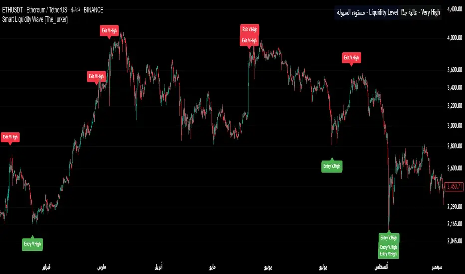
CCT Pi Cycle Top/BottomPi Cycle Top/bottom: The Ultimate Market Cycle Indicator
Introduction
The Pi Cycle Top/bottom Indicator is one of the most reliable tools for identifying Bitcoin market cycle peaks and bottoms. Its effectiveness lies in the strategic combination of moving averages that historically align with major market cycle reversals. Unlike traditional moving average crossovers, this indicator applies an advanced iterative approach to pinpoint price extremes with higher accuracy.
This version, built entirely with Pine Script™ v6, introduces unprecedented precision in detecting both the Pi Cycle Top and Pi Cycle Bottom, eliminating redundant labels, optimizing visual clarity, and ensuring the indicator adapts dynamically to evolving market conditions.
What is the Pi Cycle Theory?
The Pi Cycle Top and Pi Cycle Bottom were originally introduced based on a simple yet profound discovery: key moving average crossovers consistently align with macro market tops and bottoms.
Pi Cycle Top: The crossover of the 111-day Simple Moving Average (SMA) and the 350-day SMA multiplied by 2 has historically signaled market tops with astonishing accuracy.
Pi Cycle Bottom: The intersection of the 150-day Exponential Moving Average (EMA) and the 471-day SMA has repeatedly marked significant market bottoms.
While traditional moving average strategies often suffer from lag and false signals, the Pi Cycle Indicator enhances accuracy by applying a range-based scanning methodology, ensuring that only the most critical reversals are detected.
How This Indicator Works
Unlike basic moving average crossovers, this script introduces a unique iteration process to refine the detection of Pi Cycle points. Here’s how it works:
Detecting Crossovers:
Identifies the Golden Cross (bullish crossover) and Death Cross (bearish crossover) for both the Pi Cycle Top and Pi Cycle Bottom.
Iterating Through the Cycle:
Instead of plotting a simple crossover point, this script scans the range between each Golden and Death Cross to identify the absolute lowest price (Pi Cycle Bottom) and highest price (Pi Cycle Top) within that cycle.
Precision Labeling:
The indicator dynamically adjusts label positioning:
If the price at the crossover is below the fast moving average → the label is placed on the moving average with a downward pointer.
If the price is above the fast moving average → the label is placed below the candle with an upward pointer.
This ensures optimal visibility and prevents misleading signal placement.
Advanced Pine Script v6 Features:
Labels and moving average names are only shown on the last candle, reducing chart noise while maintaining clarity.
Offers full user customization, allowing traders to toggle:
Pi Cycle Top & Bottom visibility
Moving average labels
Crossover labels
Why This Indicator is Superior
This script is not just another moving average crossover tool—it is a market cycle tracker designed for long-term investors and analysts who seek:
✔ High-accuracy macro cycle identification
✔ Elimination of false signals using an iterative range-based scan
✔ Automatic detection of market extremes without manual adjustments
✔ Optimized visuals with smart label positioning
✔ First-of-its-kind implementation using Pine Script™ v6 capabilities
How to Use It?
Bull Market Tops:
When the Pi Cycle Top indicator flashes, consider the potential for a market cycle peak.
Historically, Bitcoin has corrected significantly after these signals.
Bear Market Bottoms:
When the Pi Cycle Bottom appears, it suggests a macro accumulation phase.
These signals have aligned perfectly with historical cycle bottoms.
Final Thoughts
The Pi Cycle Top/bottom Indicator is a must-have tool for traders, investors, and analysts looking to anticipate long-term trend reversals with precision. With its refined methodology, superior label positioning, and cutting-edge Pine Script™ v6 optimizations, this is the most reliable version ever created.
Risk MeterRisk Meter Indicator for TradingView
The Risk Meter is a powerful market risk assessment tool designed to help traders evaluate the current risk environment using a simple, data-driven score. By analyzing four critical market factors—VIX (volatility index), market breadth, trailing volatility, and credit spreads—the indicator generates a risk score between 0 and 4. This score empowers traders to make informed decisions about hedging, exiting positions, or re-entering the market, with clear visual cues and alerts for intraday monitoring.
What It Does
Calculates a Risk Score: Assigns a score from 0 to 4, where each point reflects an active risk condition based on four market indicators.
Identifies Risk Levels:
A score of 3 or higher indicates a high-risk environment, suggesting traders consider hedging or reducing exposure.
A score of 2 or lower for at least two consecutive days signals a potential opportunity to re-enter the market.
Provides Visual Feedback: Uses color-coded Columns, threshold markers, and a component table for quick interpretation.
Supports Decision-Making: Offers a structured approach to managing risk and timing trades.
How It Works
The Risk Meter aggregates four key risk conditions, each contributing 1 point to the total score when triggered:
Elevated and Rising VIX (Risk 1)
Condition: The VIX is above 18 and higher than it was 20 days ago.
Purpose: Detects increasing market fear or uncertainty.
Market Breadth Dropping (Risk 2)
Condition: Either:
Fewer than 50% of S&P 500 stocks are above their 200-day moving average and fewer than 70% are above their 50-day moving average, or
The 3-day EMA of the 200-day breadth falls below 80% of its 20-day SMA.
Purpose: Identifies weakening participation across the market.
Trailing Volatility (Risk 3)
Condition: The 30-day annualized volatility of the equal-weight S&P 500 (RSP) exceeds 35%.
Purpose: Highlights periods of heightened price instability.
Credit Spreads (Risk 4)
Condition: The price ratio of high-yield bonds (HYG) to Treasuries (TLT or IEF) is lower than it was 20 days ago, indicating widening credit spreads.
Purpose: Signals potential stress in credit markets.
The total risk score is the sum of these conditions (0 to 4). Additionally, the indicator tracks consecutive days with a score of 2 or lower to generate re-entry signals.
How to Read It Intraday
The Risk Meter is built on daily data but can be monitored intraday for real-time insights. Here’s how traders can interpret it:
Risk Score Plot:
Displayed as a step line ranging from 0 to 4.
Colors:
Red: High risk (score ≥ 3) – caution advised.
Green: Re-entry signal – score ≤ 2 for at least two consecutive days (triggered when the count increments from 1 to 2).
Blue: Neutral or low risk (score < 3 without a re-entry signal).
Threshold Lines:
Dashed Gray Line at 3: Marks the high-risk threshold.
Dotted Gray Line at 2: Indicates the low-risk threshold for re-entry signals.
Risk Component Table:
Located in the top-right corner, it lists:
VIX, Breadth, Volatility, and Credit Spreads.
Status: Shows "" (warning, red) if the risk condition is met, or "✓" (safe, blue) if not.
Helps traders pinpoint which factors are driving the score.
Alerts:
High Risk Alert: Triggers when the score moves from < 3 to ≥ 3.
Re-entry Signal Alert: Triggers when the score ≤ 2 for two consecutive days.
Intraday Usage Tips
Check the indicator throughout the day for early signs of risk shifts, especially if the score is near a threshold (e.g., 2 or 3).
Combine with other intraday tools (e.g., price action, volume) since the Risk Meter updates daily but reflects broader market conditions.
How Traders Can Use It
High-Risk Signal (Score ≥ 3):
Consider hedging positions (e.g., with options) or reducing equity exposure to protect against potential downturns.
Re-entry Signal (Score ≤ 2 for 2+ Days):
Look to re-enter the market or increase exposure, as it suggests stabilizing conditions.
Daily Risk Management:
Use the score and table to assess overall market health and adjust strategies accordingly.
Alert-Driven Trading:
Set up alerts to stay notified of critical risk changes without constant monitoring.
Why Use the Risk Meter?
This indicator offers a systematic, multi-factor approach to risk assessment, blending volatility, breadth, and credit market data into an easy-to-read score. Whether you’re an intraday trader or a longer-term investor, the Risk Meter helps you stay proactive, avoid surprises, and time your trades with greater confidence.
Financial Risk Disclaimer for the Risk Meter Tool
Important Notice: The Risk Meter is a market risk assessment tool designed to provide insights into current market conditions based on historical data and predefined indicators. It is intended for informational and educational purposes only and should not be considered financial advice, a recommendation to buy or sell any securities, or a guarantee of future market performance.
Key Considerations
No Guarantee of Accuracy: While the Risk Meter utilizes reliable data sources and established financial metrics, the creators do not guarantee the accuracy, completeness, or timeliness of the information provided. Financial markets are complex and subject to rapid, unpredictable changes, and the tool’s output may not fully reflect all market dynamics.
Market Risks: Trading and investing in financial markets carry significant risks, including the potential loss of principal. Market volatility, economic shifts, and other factors can lead to unexpected outcomes. Past performance is not a reliable indicator of future results, and the Risk Meter’s assessments are based on historical data, not future predictions.
Not a Substitute for Professional Advice: The Risk Meter is not intended to replace personalized financial guidance. Users are strongly encouraged to consult a qualified financial advisor, perform their own research, and evaluate their personal financial situation, risk tolerance, and investment objectives before making any trading or investment decisions.
Limitation of Liability: The creators of the Risk Meter, including any affiliates, developers, or contributors, are not liable for any direct, indirect, incidental, or consequential losses or damages arising from the use of this tool. This includes, but is not limited to, financial losses, missed opportunities, or decisions based on the tool’s output.
User Responsibility: By using the Risk Meter, you accept full responsibility for your trading and investment decisions. You acknowledge that you use the tool at your own risk and that the creators bear no responsibility for any outcomes resulting from its use.
Final Note
The Risk Meter is a supplementary tool designed to enhance your understanding of market risk. It is not a comprehensive solution for investment management. Approach trading and investing with caution, ensuring your decisions align with your personal financial strategy.

SatoshiSteps Swing StrategyCore Components:
The indicator combines three popular technical analysis tools:
Ichimoku Cloud: This helps identify the trend, support, and resistance levels.
RSI (Relative Strength Index): This momentum oscillator identifies overbought and oversold conditions.
MACD (Moving Average Convergence Divergence): This trend-following momentum indicator shows the relationship between two moving averages1 of prices.
Logic:
The strategy aims to identify potential swing trading opportunities by combining signals from these three components. It essentially looks for:
Trend Confirmation (Ichimoku):
Price should be above the Ichimoku cloud for buy signals.
Price should be below the Ichimoku cloud for sell signals.
The Tenkan-sen (conversion line) should cross above the Kijun-sen (base line) for buy signals.
The Tenkan-sen should cross below the Kijun-sen for sell signals.
Overbought/Oversold Conditions (RSI):
RSI should be below the overbought level for buy signals (avoiding buying when the market is potentially overextended).
RSI should be above the oversold level for sell signals (avoiding selling when the market is potentially oversold).
Momentum Confirmation (MACD):
The MACD line should be above the signal line for buy signals (indicating upward momentum).
The MACD line should be below the signal line for sell signals (indicating downward momentum).
Buy Signal:
A buy signal is generated when all the following conditions are met:
The Tenkan-sen crosses above the Kijun-sen.
The price is above both the Senkou Span A and Senkou Span B (the cloud).
The RSI is below the overbought level.
The MACD line is above the signal line.
Sell Signal:
A sell signal is generated when all the following conditions are met:
The Tenkan-sen crosses below the Kijun-sen.
The price is below both the Senkou Span A and Senkou Span B (the cloud).
The RSI is above the oversold level.
The MACD line is below the signal line.
Key Considerations:
Time Frame: The indicator has built-in adjustments for 1-hour and 4-hour timeframes, optimizing the parameters for each.
Customization: You can customize the overbought/oversold RSI levels and the styles of the buy/sell signals (triangle, label, arrow, circle) through the indicator's settings.
Accuracy: While the strategy combines multiple indicators to improve accuracy, remember that no trading indicator is perfect. Market conditions can change rapidly, and false signals can occur.
Risk Management: Always use proper risk management techniques, such as stop-loss orders, and never risk more than you can afford to lose.
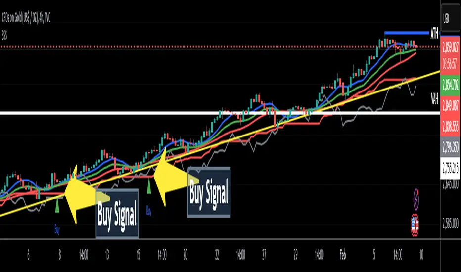
Dynamic Darvas Lines [CHE] Dynamic Darvas Lines
Unlock Precision Trading with Dynamic Darvas Lines
Overview:
Dynamic Darvas Lines is an advanced trading indicator designed for traders seeking to enhance their market analysis and decision-making process. Building upon the classic Darvas Box theory, this indicator introduces dynamic zone detection and comprehensive customization features, making it an indispensable tool for both novice and experienced traders.
Key Features & Advantages:
1. Dynamic Zone Detection:
- Adaptive Boxes: Automatically identifies and adjusts support and resistance levels based on market volatility and price movements, ensuring that the indicator remains relevant in varying market conditions.
- Real-Time Updates: Continuously recalculates box boundaries, providing up-to-the-minute insights into potential breakout or reversal points.
2. Enhanced Signal Accuracy:
- Buy & Sell Signals: Generates clear and actionable buy and sell signals based on the crossover and crossunder of price with dynamic Darvas lines, helping traders capitalize on optimal entry and exit points.
- Signal Confirmation: Reduces false signals by requiring confirmation through multiple conditions, enhancing overall trade reliability.
3. Comprehensive Customization:
- Adjustable Parameters: Tailor the indicator to your specific trading style with customizable box length, signal colors, and plot shapes.
- Color Management: Differentiate between various market signals with intuitive color coding for buy/sell signals, box boundaries, and debug lines, enhancing visual clarity on your charts.
4. Advanced Visualization:
- Signal Circles: Visual markers highlight significant price levels where buy and sell signals are triggered, making it easier to spot opportunities at a glance.
- Debug Mode: Activate debug lines to display the lowest lows and highest highs within the defined box length, aiding in in-depth market analysis and strategy refinement.
5. Robust Alert System:
- Custom Alerts: Set up real-time alerts for buy and sell signals, ensuring you never miss critical trading opportunities even when you're away from your screen.
- Automated Notifications: Receive instant notifications directly through your trading platform, keeping you informed and ready to act.
6. Seamless Integration:
- Overlay Capability: Easily integrates with your existing charts, allowing you to combine Dynamic Darvas Lines with other technical indicators for a more comprehensive market view.
- Optimized Performance: Efficiently coded in Pine Script V5, ensuring smooth performance without lag, even on lower-end devices.
Use Cases:
- Trend Identification: Detect and follow market trends by observing the formation and breakout of dynamic Darvas boxes, helping you stay aligned with the market’s momentum.
- Breakout Trading: Capitalize on significant price movements when the price breaks out of established Darvas zones, indicating potential strong directional moves.
- Reversal Detection: Identify potential market reversals by monitoring when the price crosses under the lower Darvas line or above the upper Darvas line, signaling a change in market sentiment.
- Risk Management: Utilize the indicator’s clear support and resistance levels to set strategic stop-loss and take-profit points, enhancing your risk-reward ratio.
- Market Analysis: Combine with other technical tools and indicators to perform comprehensive market analysis, improving the accuracy of your trading strategies.
Why Choose Dynamic Darvas Lines ?
Dynamic Darvas Lines stands out with its blend of traditional Darvas Box principles and modern enhancements. Its dynamic nature ensures adaptability across different market conditions, while the extensive customization options provide traders with the flexibility to tailor the indicator to their unique trading strategies. Whether you’re aiming to identify trends, execute breakout trades, or manage risks more effectively, Dynamic Darvas Lines offers the precision and reliability you need to elevate your trading game.
Get Started Today:
Enhance your trading toolkit with Dynamic Darvas Lines and experience the difference in your market analysis and trading performance. Download now and take the first step towards more informed and strategic trading decisions!
Note: Always backtest any trading indicator and use it in conjunction with other analysis tools to develop a robust trading strategy. Trading involves risk, and it's essential to practice sound risk management.
Disclaimer:
The content provided, including all code and materials, is strictly for educational and informational purposes only. It is not intended as, and should not be interpreted as, financial advice, a recommendation to buy or sell any financial instrument, or an offer of any financial product or service. All strategies, tools, and examples discussed are provided for illustrative purposes to demonstrate coding techniques and the functionality of Pine Script within a trading context.
Any results from strategies or tools provided are hypothetical, and past performance is not indicative of future results. Trading and investing involve high risk, including the potential loss of principal, and may not be suitable for all individuals. Before making any trading decisions, please consult with a qualified financial professional to understand the risks involved.
By using this script, you acknowledge and agree that any trading decisions are made solely at your discretion and risk.
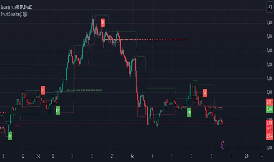
Adaptive MA Scalping StrategyAdaptive MA Scalping Strategy
The Adaptive MA Scalping Strategy is an innovative trading approach that merges the strengths of the Kaufman's Adaptive Moving Average (KAMA) with the Moving Average Convergence Divergence (MACD) histogram. This combination results in a momentum-adaptive moving average that dynamically adjusts to market conditions, providing traders with timely and reliable signals.
How It Works
Kaufman's Adaptive Moving Average (KAMA): Unlike traditional moving averages, KAMA adjusts its sensitivity based on market volatility. It becomes more responsive during trending markets and less sensitive during periods of consolidation, effectively filtering out market noise.
MACD Histogram Integration: The strategy incorporates the MACD histogram, a momentum indicator that measures the difference between a fast and a slow exponential moving average (EMA). By adding the MACD histogram values to the KAMA, the strategy creates a new line—the momentum-adaptive moving average (MOMA)—which captures both trend direction and momentum.
Signal Generation:
Long Entry: The strategy enters a long position when the closing price crosses above the MOMA. This indicates a potential upward momentum shift.
Exit Position: The position is closed when the closing price crosses below the MOMA, signaling a potential decline in momentum.
Cloud Calculation Detail
The MOMA is calculated by adding the MACD histogram value to the KAMA of the price. This addition effectively adjusts the KAMA based on the momentum indicated by the MACD histogram. When momentum is strong, the MACD histogram will have higher values, causing the MOMA to adjust accordingly and provide earlier entry or exit signals.
Performance on Stocks
This strategy has demonstrated excellent performance on stocks when applied to the 1-hour timeframe. Its adaptive nature allows it to respond swiftly to market changes, capturing profitable trends while minimizing the impact of false signals caused by market noise. The combination of KAMA's adaptability and MACD's momentum detection makes it particularly effective in volatile market conditions commonly seen in stock trading.
Key Parameters
KAMA Length (malen): Determines the sensitivity of the KAMA. A length of 100 is used to balance responsiveness with noise reduction.
MACD Fast Length (fast): Sets the period for the fast EMA in the MACD calculation. A value of 24 helps in capturing short-term momentum changes.
MACD Slow Length (slow): Sets the period for the slow EMA in the MACD calculation. A value of 52 smooths out longer-term trends.
MACD Signal Length (signal): Determines the period for the signal line in the MACD calculation. An 18-period signal line is used for timely crossovers.
Advantages of the Strategy
Adaptive to Market Conditions: By adjusting to both volatility and momentum, the strategy remains effective across different market phases.
Enhanced Signal Accuracy: The fusion of KAMA and MACD reduces false signals, improving the accuracy of trade entries and exits.
Simplicity in Execution: With straightforward entry and exit rules based on price crossovers, the strategy is user-friendly for traders at all experience levels

[Suitable Hope] Crypto Upside Model 3.0The "Crypto Upside Model 3.0" indicator dynamically calculates the potential price of any cryptocurrency based on various percentages of Ethereum or Bitcoin's market capitalization.
By fetching and analyzing marketcap data from TradingView sources, it allows traders to visualize potential price targets if their chosen cryptocurrency reaches specific market dominance levels. This tool is designed for daily timeframe analysis and can be used to set informed price expectations and strategic investment goals, providing valuable insights for long-term investment planning.
Why using the Crypto Upside Model 3.0?
Strategic Planning: Helps traders and investors set realistic price targets and investment goals by visualizing potential market cap scenarios.
Informed Decision-Making: Provides a data-driven approach to understanding how a cryptocurrency might perform relative to major assets like Bitcoin and Ethereum.
Customizable Analysis: Allows users to choose different comparison assets (ETH or BTC) and visualize various market cap dominance percentages, offering tailored insights.
Daily Timeframe Focus: Ideal for swing traders and long-term investors who operate on a daily analysis timeframe, providing relevant and actionable data.
Bull Markets: Identify potential price targets if your cryptocurrency's market cap increases significantly.
Bear Markets: Assess how much value could be retained relative to major cryptocurrencies.
Strategic Entry/Exit Points: Use the visualized targets to plan entry or exit points in your trading strategy.
Comparative Advantage
Dynamic Adaptation: Unlike fixed indicators, this tool adapts to any active chart, making it versatile for multiple cryptocurrencies.
Market Cap Insights: Provides a unique perspective by linking price targets to market cap dominance, a critical factor in the crypto market.
User Instructions
Setup: Add the " Upside Model 3.0" indicator to your TradingView chart.
Configuration: Use the input settings to select the comparison cryptocurrency (ETH or BTC) and enable the desired market cap percentage plots.
Analysis: The indicator will display potential price targets based on the selected market cap percentages, providing a visual guide for setting price expectations.
Limitations
Marketcap Data Availability: The indicator relies on marketcap data from TradingView, which may not be available for all cryptocurrencies. If the data is unavailable, the indicator will not function for that asset. This tool is more likely to work with older, established cryptocurrencies, as marketcap data for newer cryptocurrencies may not yet be available.
Daily Timeframe Restriction: The indicator is designed to work exclusively on the daily timeframe, limiting its applicability for intraday trading.
Assumptions of Market Dynamics: The calculations assume a direct correlation between market dominance and price, which may not account for other market dynamics and external factors influencing prices.
Data Accuracy: The accuracy of the indicator depends on the reliability of the data provided by TradingView, which may sometimes experience delays or inaccuracies.
Currently available cryptocurrencies: Bitcoin, Ethereum, Solana, Binance Coin, Cardano, Ripple, Polkadot, Avalanche, Chainlink, Litecoin, Dogecoin, Terra, Uniswap, VeChain, Stellar, Internet Computer, Hedera, Filecoin, Monero, Aave, TRON, NEAR Protocol, Compound, Maker,... For all compatible cryptocurrencies, please consult CRYPTOCAP's documentation.
Final notes
Although various sources ask a payment or user data for similar kind of private indicators, this one is entirely free and open source. "Uncanny" isn't it? I hope this indicator will provide you value. Feel free to leave a message if you have any questions or constructive feedback.
Examples of how I use this indicator
When using ETH's historical price as a reference compared to Bitcoin's marketcap, we can notice that price generally has been held between the +-30% and 50% lines of BTC's marketcap. If history is repeating again, we can expect major resistances around the 50% looking ahead into the future. This for me would be a great area to potentially reduce my ETH spot position.
When using SOL's historical price action, we can notice that the 15% line of ETH's marketcap has been a top in the previous cycle. Today SOL (July 2024), is back at this level. Could this be a top again or could price break this 15% level and head perhaps towards 30% which currently sits around $260? Time will tell.
These are 2 simple example of how I interpret the data. I'm keen to hear what other findings with other pairs you can find.