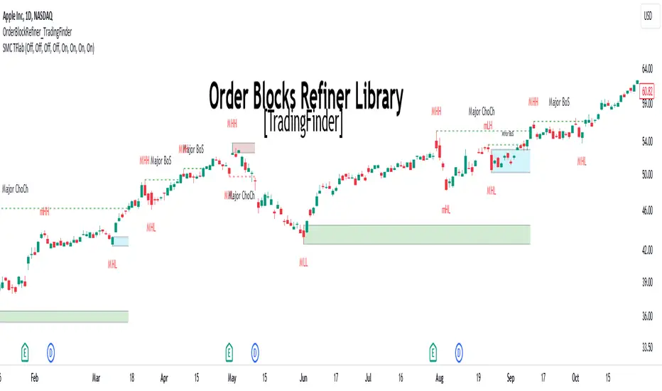
Order Block Refiner [TradingFinder]🔵 Introduction
The "Refinement" feature allows you to adjust the width of the order block according to your strategy. There are two modes, "Aggressive" and "Defensive," in the "Order Block Refine". The difference between "Aggressive" and "Defensive" lies in the width of the order block.
For risk-averse traders, the "Defensive" mode is suitable as it provides a lower loss limit and a greater reward-to-risk ratio. For risk-taking traders, the "Aggressive" mode is more appropriate. These traders prefer to enter trades at higher prices, and this mode, which has a wider order block width, is more suitable for this group of individuals.
Important :
One of the advantages of using this library is increased code accuracy. Not only does it have the capability to create order blocks, but you can also simply define the condition for order block creation (true/false) and "bar_index," and you'll find the primary range without applying any filters.
🟣 Order Block Refinement Algorithm
The order block ranges are filtered in two stages. In the first stage, the "Open," "High," "Low," and "Close" of the current order block candle, its two or three previous candles, and one subsequent candle (if available) are examined. In this stage, minimum and maximum distances are calculated, and logical range filters are applied.
In the second stage, two modes, "Aggressive" and "Defensive," are calculated.
For the "Defensive" mode, the width of these ranges is compared with the "ATR" (Average True Range) of period 55, and if they are smaller than "ATR" or 1 to more than 4 times "ATR," the width of the range is reduced from 0 to 80 percent.
For the "Aggressive" mode, you get the same output as the first filter, which usually has a wider width than the "Defensive" mode.
• Order Block Refiner : Off
• Order Block Refiner : On / "Aggressive Mode"
• Order Block Refiner : On / "Defensive Mode"
🔵 How to Use
OBRefiner(string OBType, string OBRefine, string RefineMethod, bool TriggerCondition, int Index) =>
Parameters:
• OBType (string)
• OBRefine (string)
• RefineMethod (string)
• TriggerCondition (bool)
• Index (int)
To add "Order Block Refiner Library", you must first add the following code to your script.
import TFlab/OrderBlockRefiner_TradingFinder/1
OBType : This parameter receives 2 inputs. If the order block you want to "Refine" is of type demand, you should enter "Demand," and if it's of type supply, you should enter "Supply."
OBRefine : Set to "On" if you want the "Refine" operation to be performed. Otherwise, set to "Off."
RefineMethod : This input receives 2 modes, "Aggressive" and "Defensive." You can switch between these modes according to your needs.
TriggerCondition : Enter the condition with which the order block is formed in this parameter.
Index : Enter the "bar_index" of the candle where the order block is formed in this parameter.
🟣 Function Outputs
This function has 6 outputs: "bar_index" at the beginning of the "Distal" line, "bar_index+1" at the end of the "Distal" line, "Price" at the "Distal" line, "bar_index" at the beginning of the "Proximal" line, "bar_index+1" at the end of the "Proximal" line, and "Price" at the "Proximal" line, which can be used to draw order blocks.
Sample :
= Refiner.OBRefiner('Demand', 'Off', 'Aggressive',BuMChMain_Trigger, BuMChMain_Index)
if BuMChMain_Trigger
BuMChHlineMain := line.new(BuMChMain_Xp1 , BuMChMain_Yp12 , bar_index , BuMChMain_Yp12, color = color.black , style = line.style_dotted)
BuMChLlineMain := line.new(BuMChMain_Xd1 , BuMChMain_Yd12 , bar_index , BuMChMain_Yd12, color = color.black , style = line.style_dotted)
BuMChFilineMain := linefill.new(BuMChHlineMain ,BuMChLlineMain , color = color.rgb(76, 175, 80 , 75 ) )
Cerca negli script per "accuracy"
Unmitigated Liquidity Imbalances [AlgoAlpha]🎉 Introducing the Unmitigated Liquidity Imbalance Indicator by AlgoAlpha! 🎉
Dive into the depths of market analytics with our "Unmitigated Liquidity Imbalance" indicator. This tool harnesses unique algorithms to detect liquidity imbalances between bulls and bears, helping traders spot trends and potential entry and exit points with greater accuracy. 📈🚀
🔍 Key Features:
🌟 Advanced Analysis : Analyses candle direction and length to forecast market peaks and valleys.
🎨 Customizable Visuals : Tailor the chart with your choice of bullish green or bearish red to reflect different market conditions.
🔄 Real-Time Updates : Continuously updates to reflect live market changes.
🔔 Configurable Alerts : Set up alerts for key trading signals such as bullish and bearish reversals, as well as trend shifts.
📐 How to Use:
🛠 Add the Indicator : Add the indicator to your favourites and customize the settings to suite your needs.
📊 Market Analysis : Monitor the oscillator threshold; readings above 0.5 suggest bullish sentiment, while below 0.5 indicate bearish conditions. And reversal signals are displayed to show potential entry points.
🔔 Set Alerts : Enable notifications for reversal conditions or trend changes to seize trading opportunities without constant chart watching.
🧠 How It Works:
The core mechanism of the indicator is based on detecting changes in candlestick size and direction to identify bullish and bearish liquidity levels from the peak & valley indicator's logic. By comparing the length of a current candle to the previous one and checking the change in direction, it pinpoints moments where market sentiment could be shifting, indicating if the liquidity at that point is bullish or bearish. The script then looks at what percentage of the past few unmitigated levels are bullish or bearish based on a customizable lookback and determines the liquidity imbalance which can then be interpreted as trend.
Empower your trading with the Unmitigated Liquidity Imbalance indicator and navigate the markets with confidence and precision. 🌟💹
Happy trading, and may your charts be ever in your favour! 🥳✨
💎 Related Indicator

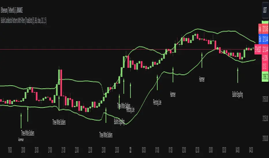
Bullish Candlestick Patterns With Filters [TradeDots]The "Bullish Candlestick Patterns With Filters" is a trading indicator that identifies 6 core bullish candlestick patterns. This is further enhanced by applying channel indicator as filters, designed to further increase the accuracy of the recognized patterns.
6 CANDLESTICK PATTERNS
Hammer
Inverted Hammer
Bullish Engulfing
The Piercing Line
The Morning Star
The 3 White Soldiers
SIGNAL FILTERING
The indicator incorporates with 2 primary methodologies aimed at filtering out lower accuracy signals.
Firstly, it comes with a "Lowest period" parameter that examines whether the trough of the bullish candlestick configuration signifies the lowest point within a specified retrospective bar length. The longer the period, the higher the probability that the price will rebound.
Secondly, the channel indicators, the Keltner Channels or Bollinger Bands. This indicator examines whether the lowest point of the bullish candlestick pattern breaches the lower band, indicating an oversold signal. Users have the flexibility to modify the length and band multiplier, enabling them to custom-tune signal sensitivity.
Without Filtering:
With Filtering
RISK DISCLAIMER
Trading entails substantial risk, and most day traders incur losses. All content, tools, scripts, articles, and education provided by TradeDots serve purely informational and educational purposes. Past performances are not definitive predictors of future results.
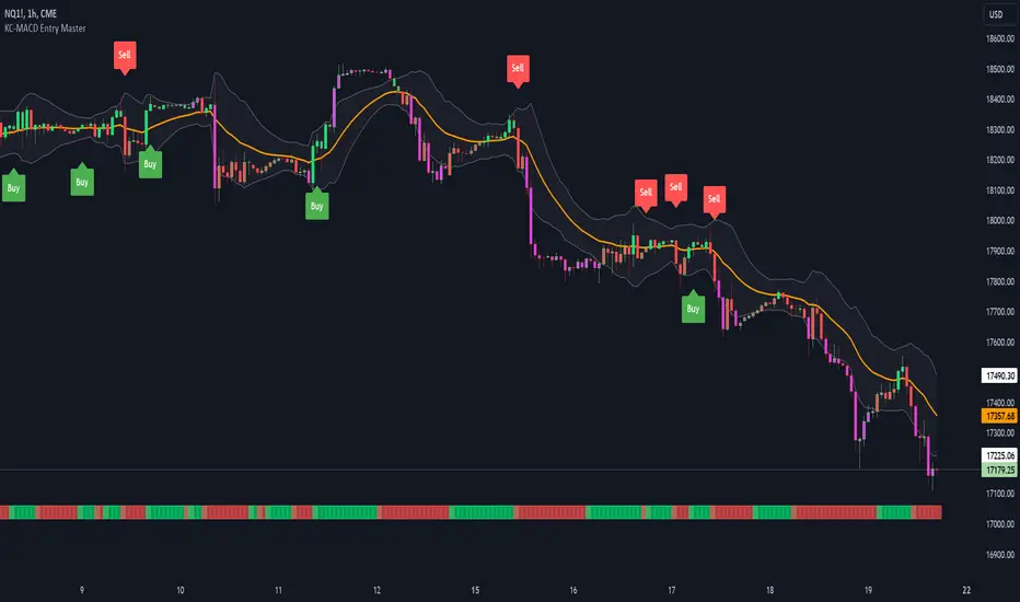
KC-MACD Entry Master @shrilssThe KC-MACD Entry Master is designed to enhance trading strategies by utilizing Keltner Channels and MACD for dynamic market analysis. This indicator excels in visually identifying market conditions with a sophisticated bar coloring system and an informative MACD Traffic Light feature.
Key Features:
- Dynamic Bar Coloring: The core feature of this indicator is its ability to adjust the color of bars based on their positioning relative to the Keltner Channels and the EMA (Exponential Moving Average). It colors bars lime or red when the closing price is within the Keltner Channels but above or below the EMA, respectively. Additionally, it uses a fuchsia color to indicate breakouts when the price extends beyond the Keltner Channels. This visual aid helps traders quickly identify potential buying or selling opportunities based on market volatility and price action.
- MACD Traffic Light: Positioned at the bottom of the chart, this unique feature displays the histogram color of the MACD, set by default to a 3/10/16 configuration—known as the 3-10 Oscillator. This Traffic Light gives traders an at-a-glance view of the underlying momentum and trend shifts, further aiding in decision-making processes.
- MACD-Based Entry Signals: By calculating the fast and slow moving averages specified by the user, the script determines MACD values and their crossover with a smoothed signal line. Entry points are then highlighted with shapes (e.g., "Buy" or "Sell") plotted on the chart when conditions are met, including alignment with the bar colors for enhanced accuracy.
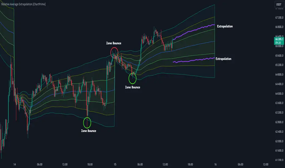
Relative Average Extrapolation [ChartPrime]Relative Average Extrapolation (ChartPrime) is a new take on session averages, like the famous vwap . This indicator leverages patterns in the market by leveraging average-at-time to get a footprint of the average market conditions for the current time. This allows for a great estimate of market conditions throughout the day allowing for predictive forecasting. If we know what the market conditions are at a given time of day we can use this information to make assumptions about future market conditions. This is what allows us to estimate an entire session with fair accuracy. This indicator works on any intra-day time frame and will not work on time frames less than a minute, or time frames that are a day or greater in length. A unique aspect of this indicator is that it allows for analysis of pre and post market sessions independently from regular hours. This results in a cleaner and more usable vwap for each individual session. One drawback of this is that the indicator utilizes an average for the length of a session. Because of this, some after hour sessions will only have a partial estimation. The average and deviation bands will work past the point where it has been extrapolated to in this instance however. On low time frames due to the limited number of data points, the indicator can appear noisy.
Generally crypto doesn't have a consistent footprint making this indicator less suitable in crypto markets. Because of this we have implemented other weighting schemes to allow for more flexibility in the number of use cases for this indicator. Besides volume weighting we have also included time, volatility, and linear (none) weighting. Using any one of these weighting schemes will transform the vwap into a wma, volatility adjusted ma, or a simple moving average. All of the style are still session period and will become longer as the session progresses.
Relative Average Extrapolation (ChartPrime) works by storing data for each time step throughout the day by utilizing a custom indexing system. It takes the a key , ie hour/minute, and transforms it into an array index to stor the current data point in its unique array. From there we can take the current time of day and advance it by one step to retrieve the data point for the next bar index. This allows us to utilize the footprint the extrapolate into the future. We use the relative rate of change for the average, the relative deviation, and relative price position to extrapolate from the current point to the end of the session. This process is fast and effective and possibly easier to use than the built in map feature.
If you have used vwap before you should be familiar with the general settings for this indicator. We have made a point to make it as intuitive for anyone who is already used to using the standard vwap. You can pick the source for the average and adjust/enable the deviation bands multipliers in the settings group. The average period is what determines the number of days to use for the average-at-time. When it is set to 0 it will use all available data. Under "Extrapolation" you will find the settings for the estimation. "Direction Sensitivity" adjusts how sensitive the indicator is to the direction of the vwap. A higher number will allow it to change directions faster, where a lower number will make it more stable throughout the session. Under the "Style" section you will find all of the color and style adjustments to customize the appearance of this indicator.
Relative Average Extrapolation (ChartPrime) is an advanced and customizable session average indicator with the ability to estimate the direction and volatility of intra-day sessions. We hope you will find this script fascinating and useful in your trading and decision making. With its unique take on session weighting and forecasting, we believe it will be a secret weapon for traders for years to come.
Enjoy
US CPIIntroducing "US CPI" Indicator
The "US CPI" indicator, based on the Consumer Price Index (CPI) of the United States, is a valuable tool for analyzing inflation trends in the U.S. economy. This indicator is derived from official data provided by the U.S. Bureau of Labor Statistics (BLS) and is widely recognized as a key measure of inflationary pressures.
What is CPI?
The Consumer Price Index (CPI) is a measure that examines the average change in prices paid by consumers for a basket of goods and services over time. It is an essential economic indicator used to gauge inflationary trends and assess changes in the cost of living.
How is "US CPI" Calculated?
The "US CPI" indicator in this script retrieves CPI data from the Federal Reserve Economic Data (FRED) using the FRED:CPIAUCSL symbol. It calculates the rate of change in CPI over a specified period (typically 12 months) and applies technical analysis tools like moving averages (SMA and EMA) for trend analysis and smoothing.
Why Use "US CPI" Indicator?
1. Inflation Analysis: Monitoring CPI trends provides insights into the rate of inflation, which is crucial for understanding the overall economic health and potential impact on monetary policy.
2. Policy Implications: Changes in CPI influence decisions by policymakers, central banks, and investors regarding interest rates, fiscal policies, and asset allocation.
3. Market Sentiment: CPI data often impacts market sentiment, influencing trading strategies across various asset classes including currencies, bonds, and equities.
Key Features:
1. Customizable Smoothing: The indicator allows users to apply exponential moving average (EMA) smoothing to CPI data for clearer trend identification.
2. Visual Representation: The plotted line visually represents the inflation rate based on CPI data, helping traders and analysts assess inflationary pressures at a glance.
Sources and Data Integrity:
The CPI data used in this indicator is sourced directly from FRED, ensuring reliability and accuracy. The script incorporates robust security protocols to handle data requests and maintain data integrity in a trading environment.
In conclusion, the "US CPI" indicator offers a comprehensive view of inflation dynamics in the U.S. economy, providing traders, economists, and policymakers with valuable insights for informed decision-making and risk management.
Disclaimer: This indicator and accompanying analysis are for informational purposes only and should not be construed as financial advice. Users are encouraged to conduct their own research and consult with professional advisors before making investment decisions.

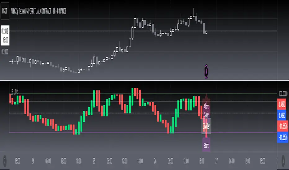
[blackcat] L3 Ultimate Market Sentinel (UMS)Script Introduction
The L3 Ultimate Market Sentinel (UMS) is a technical indicator specifically designed to capture market turning points. This indicator incorporates the principles of the Stochastic Oscillator and provides a clear view of market dynamics through four key boundary lines — the Alert Line, Start Line, Safe Line, and Divider Line. The UMS indicator not only focuses on the absolute movement of prices but also visually displays subtle changes in market sentiment through color changes (green for rise, red for fall), helping traders quickly identify potential buy and sell opportunities.
In the above image, you can see how the UMS indicator labels different market conditions on the chart. Green candlestick charts indicate price increases, while red candlestick charts indicate price decreases. The Alert Line (Alert Line) is typically set at a higher level to warn of potential overheating in the market; the Start Line (Start Line) is in the middle, marking the beginning of market momentum; the Safe Line (Safe Line) is at a lower level, indicating a potential oversold state in the market; the Divider Line (Divider Line) helps traders identify whether the market is in an overbought or oversold area.
Script Usage
1. **Identifying Turning Points**: Traders should pay close attention to the Alert Line and Safe Line in the UMS indicator. When the indicator approaches or touches the Alert Line, it may signal an imminent market reversal; when the indicator touches the Safe Line, it may indicate that the market is oversold and there is a chance for a rebound.
2. **Color Changes**: By observing the color changes in the histogram, traders can quickly judge market trends. The transition from green to red may indicate a weakening of upward momentum, while the shift from red to green could suggest a slowdown in downward momentum.
3. **Trading Strategy**: The UMS indicator is suitable for a variety of trading timeframes, ranging from 1 minute to 1 hour. Short-term traders can use the UMS indicator to capture rapid market fluctuations, while medium-term traders can combine it with other analytical tools to confirm the sustainability of trends.
Advantages and Limitations of the Indicator
**Advantages**:
- Intuitive color coding that is easy to understand and use.
- Multiple boundary lines provide comprehensive market analysis.
- Suitable for a variety of trading timeframes, offering high flexibility.
**Limitations**:
- As a single indicator, it may not cover all market dynamics.
- For novice traders, it may be necessary to use the UMS indicator in conjunction with other indicators to improve accuracy.
- The indicator may lag in extreme market conditions.
Special Note
The L3 Ultimate Market Sentinel (UMS) indicator is a powerful analytical tool, but it is not omnipotent. The market has its inherent risks and uncertainties, so it is recommended that traders use the UMS indicator in conjunction with their own trading strategies and risk management rules. Additionally, it is always recommended to fully test and verify any indicator in a simulated environment before actual application.
Kalman Hull Supertrend [BackQuant]Kalman Hull Supertrend
At its core, this indicator uses a Kalman filter of price, put inside of a hull moving average function (replacing the weighted moving averages) and then using that as a price source for the supertrend instead of the normal hl2 (high+low/2).
Therefore, making it more adaptive to price and also sensitive to recent price action.
PLEASE Read the following, knowing what an indicator does at its core before adding it into a system is pivotal. The core concepts can allow you to include it in a logical and sound manner.
1. What is a Kalman Filter
The Kalman Filter is an algorithm renowned for its efficiency in estimating the states of a linear dynamic system amidst noisy data. It excels in real-time data processing, making it indispensable in fields requiring precise and adaptive filtering, such as aerospace, robotics, and financial market analysis. By leveraging its predictive capabilities, traders can significantly enhance their market analysis, particularly in estimating price movements more accurately.
If you would like this on its own, with a more in-depth description please see our Kalman Price Filter.
2. Hull Moving Average (HMA) and Its Core Calculation
The Hull Moving Average (HMA) improves on traditional moving averages by combining the Weighted Moving Average's (WMA) smoothness and reduced lag. Its core calculation involves taking the WMA of the data set and doubling it, then subtracting the WMA of the full period, followed by applying another WMA on the result over the square root of the period's length. This methodology yields a smoother and more responsive moving average, particularly useful for identifying market trends more rapidly.
3. Combining Kalman Filter with HMA
The innovative combination of the Kalman Filter with the Hull Moving Average (KHMA) offers a unique approach to smoothing price data. By applying the Kalman Filter to the price source before its incorporation into the HMA formula, we enhance the adaptiveness and responsiveness of the moving average. This adaptive smoothing method reduces noise more effectively and adjusts more swiftly to price changes, providing traders with clearer signals for market entries or exits.
The calculation is like so:
KHMA(_src, _length) =>
f_kalman(2 * f_kalman(_src, _length / 2) - f_kalman(_src, _length), math.round(math.sqrt(_length)))
4. Integration with Supertrend
Incorporating this adaptive price smoothing technique into the Supertrend indicator further enhances its efficiency. The Supertrend, known for its proficiency in identifying the prevailing market trend and providing clear buy or sell signals, becomes even more powerful with an adaptive price source. This integration allows the Supertrend to adjust more dynamically to market changes, offering traders more accurate and timely trading signals.
5. Application in a Trading System
In a trading system, the Kalman Hull Supertrend indicator can serve as a critical component for identifying market trends and generating signals for potential entry and exit points. Its adaptiveness and sensitivity to price changes make it particularly useful for traders looking to minimize lag in signal generation and improve the accuracy of their market trend analysis. Whether used as a standalone tool or in conjunction with other indicators, its dynamic nature can significantly enhance trading strategies.
6. Core Calculations and Benefits
The core of this indicator lies in its sophisticated filtering and averaging techniques, starting with the Kalman Filter's predictive adjustments, followed by the adaptive smoothing of the Hull Moving Average, and culminating in the trend-detecting capabilities of the Supertrend. This multi-layered approach not only reduces market noise but also adapts to market volatility more effectively. Benefits include improved signal accuracy, reduced lag, and the ability to discern trend changes more promptly, offering traders a competitive edge.
Thus following all of the key points here are some sample backtests on the 1D Chart
Disclaimer: Backtests are based off past results, and are not indicative of the future.
INDEX:BTCUSD
INDEX:ETHUSD
BINANCE:SOLUSD

TrippleMACDCryptocurrency Scalping Strategy for 1m Timeframe
Introduction:
Welcome to our cutting-edge cryptocurrency scalping strategy tailored specifically for the 1-minute timeframe. By combining three MACD indicators with different parameters and averaging them, along with applying RSI, we've developed a highly effective strategy for maximizing profits in the cryptocurrency market. This strategy is designed for automated trading through our bot, which executes trades using hooks. All trades are calculated for long positions only, ensuring optimal performance in a fast-paced market.
Key Components:
MACD (Moving Average Convergence Divergence):
We've utilized three MACD indicators with varying parameters to capture different aspects of market momentum.
Averaging these MACD indicators helps smooth out noise and provides a more reliable signal for trading decisions.
RSI (Relative Strength Index):
RSI serves as a complementary indicator, providing insights into the strength of bullish trends.
By incorporating RSI, we enhance the accuracy of our entry and exit points, ensuring timely execution of trades.
Strategy Overview:
Long Position Entries:
Initiate long positions when all three MACD indicators signal bullish momentum and the RSI confirms bullish strength.
This combination of indicators increases the probability of successful trades, allowing us to capitalize on uptrends effectively.
Utilizing Linear Regression:
Linear regression is employed to identify consolidation phases in the market.
Recognizing consolidation periods helps us avoid trading during choppy price action, ensuring optimal performance.
Suitability for Grid Trading Bots:
Our strategy is well-suited for grid trading bots due to frequent price fluctuations and opportunities for grid activation.
The strategy's design accounts for price breakthroughs, which are advantageous for grid trading strategies.
Benefits of the Strategy:
Consistent Performance Across Cryptocurrencies:
Through rigorous testing on various cryptocurrency futures contracts, our strategy has demonstrated favorable results across different coins.
Its adaptability makes it a versatile tool for traders seeking consistent profits in the cryptocurrency market.
Integration of Advanced Techniques:
By integrating multiple indicators and employing linear regression, our strategy leverages advanced techniques to enhance trading performance.
This strategic approach ensures a comprehensive analysis of market conditions, leading to well-informed trading decisions.
Conclusion:
Our cryptocurrency scalping strategy offers a sophisticated yet user-friendly approach to trading in the fast-paced environment of the 1-minute timeframe. With its emphasis on automation, accuracy, and adaptability, our strategy empowers traders to navigate the complexities of the cryptocurrency market with confidence. Whether you're a seasoned trader or a novice investor, our strategy provides a reliable framework for achieving consistent profits and maximizing returns on your investment.

Kalman Filtered RSI Oscillator [BackQuant]Kalman Filtered RSI Oscillator
The Kalman Filtered RSI Oscillator is BackQuants new free indicator designed for traders seeking an advanced, empirical approach to trend detection and momentum analysis. By integrating the robustness of a Kalman filter with the adaptability of the Relative Strength Index (RSI), this tool offers a sophisticated method to capture market dynamics. This indicator is crafted to provide a clearer, more responsive insight into price trends and momentum shifts, enabling traders to make informed decisions in fast-moving markets.
Core Principles
Kalman Filter Dynamics:
At its core, the Kalman Filtered RSI Oscillator leverages the Kalman filter, renowned for its efficiency in predicting the state of linear dynamic systems amidst uncertainties. By applying it to the RSI calculation, the tool adeptly filters out market noise, offering a smoothed price source that forms the basis for more accurate momentum analysis. The inclusion of customizable parameters like process noise, measurement noise, and filter order allows traders to fine-tune the filter’s sensitivity to market changes, making it a versatile tool for various trading environments.
RSI Adaptation:
The RSI is a widely used momentum oscillator that measures the speed and change of price movements. By integrating the RSI with the Kalman filter, the oscillator not only identifies the prevailing trend but also provides a smoothed representation of momentum. This synergy enhances the indicator's ability to signal potential reversals and trend continuations with a higher degree of reliability.
Advanced Smoothing Techniques:
The indicator further offers an optional smoothing feature for the RSI, employing a selection of moving averages (HMA, THMA, EHMA, SMA, EMA, WMA, TEMA, VWMA) for traders seeking to reduce volatility and refine signal clarity. This advanced smoothing mechanism is pivotal for traders looking to mitigate the effects of short-term price fluctuations on the RSI's accuracy.
Empirical Significance:
Empirically, the Kalman Filtered RSI Oscillator stands out for its dynamic adjustment to market conditions. Unlike static indicators, the Kalman filter continuously updates its estimates based on incoming price data, making it inherently more responsive to new market information. This dynamic adaptation, combined with the RSI's momentum analysis, offers a powerful approach to understanding market trends and momentum with a depth not available in traditional indicators.
Trend Identification and Momentum Analysis:
Traders can use the Kalman Filtered RSI Oscillator to identify strong trends and momentum shifts. The color-coded RSI columns provide immediate visual cues on the market's direction and strength, aiding in quick decision-making.
Optimal for Various Market Conditions:
The flexibility in tuning the Kalman filter parameters makes this indicator suitable for a wide range of assets and market conditions, from volatile to stable markets. Traders can adjust the settings based on empirical testing to find the optimal configuration for their trading strategy.
Complementary to Other Analytical Tools:
While powerful on its own, the Kalman Filtered RSI Oscillator is best used in conjunction with other analytical tools and indicators. Combining it with volume analysis, price action patterns, or other trend-following indicators can provide a comprehensive view of the market, allowing for more nuanced and informed trading decisions.
The Kalman Filtered RSI Oscillator is a groundbreaking tool that marries empirical precision with advanced trend analysis techniques. Its innovative use of the Kalman filter to enhance the RSI's performance offers traders an unparalleled ability to navigate the complexities of modern financial markets. Whether you're a novice looking to refine your trading approach or a seasoned professional seeking advanced analytical tools, the Kalman Filtered RSI Oscillator represents a significant step forward in technical analysis capabilities.
Thus following all of the key points here are some sample backtests on the 1D Chart
Disclaimer: Backtests are based off past results, and are not indicative of the future.
INDEX:BTCUSD
INDEX:ETHUSD
BINANCE:SOLUSD

Adaptive Moving Average (AMA) Signals (Zeiierman)█ Overview
The Adaptive Moving Average (AMA) Signals indicator, enhances the classic concept of moving averages by making them adaptive to the market's volatility. This adaptability makes the AMA particularly useful in identifying market trends with varying degrees of volatility.
The core of the AMA's adaptability lies in its Efficiency Ratio (ER), which measures the directionality of the market over a given period. The ER is calculated by dividing the absolute change in price over a period by the sum of the absolute differences in daily prices over the same period.
⚪ Why It's Useful
The AMA Signals indicator is particularly useful because of its adaptability to changing market conditions. Unlike static moving averages, it dynamically adjusts, providing more relevant signals that can help traders capture trends earlier or identify reversals with greater accuracy. Its configurability makes it suitable for various trading strategies and timeframes, from day trading to swing trading.
█ How It Works
The AMA Signals indicator operates on the principle of adapting to market efficiency through the calculation of the Efficiency Ratio (ER), which measures the directionality of the market over a specified period. By comparing the net price change to total price movements, the AMA adjusts its sensitivity, becoming faster during trending markets and slower during sideways markets. This adaptability is enhanced by a gamma parameter that filters signals for either trend continuation or reversal, making it versatile across different market conditions.
change = math.abs(close - close )
volatility = math.sum(math.abs(close - close ), n)
ER = change / volatility
Efficiency Ratio (ER) Calculation: The AMA begins with the computation of the Efficiency Ratio (ER), which measures the market's directionality over a specified period. The ER is a ratio of the net price change to the total price movements, serving as a measure of the efficiency of price movements.
Adaptive Smoothing: Based on the ER, the indicator calculates the smoothing constants for the fastest and slowest Exponential Moving Averages (EMAs). These constants are then used to compute a Scaled Smoothing Coefficient (SC) that adapts the moving average to the market's efficiency, making it faster during trending periods and slower in sideways markets.
Signal Generation: The AMA applies a filter, adjusted by a "gamma" parameter, to identify trading signals. This gamma influences the sensitivity towards trend or reversal signals, with options to adjust for focusing on either trend-following or counter-trend signals.
█ How to Use
Trend Identification: Use the AMA to identify the direction of the trend. An upward moving AMA indicates a bullish trend, while a downward moving AMA suggests a bearish trend.
Trend Trading: Look for buy signals when the AMA is trending upwards and sell signals during a downward trend. Adjust the fast and slow EMA lengths to match the desired sensitivity and timeframe.
Reversal Trading: Set the gamma to a positive value to focus on reversal signals, identifying potential market turnarounds.
█ Settings
Period for ER calculation: Defines the lookback period for calculating the Efficiency Ratio, affecting how quickly the AMA responds to changes in market efficiency.
Fast EMA Length and Slow EMA Length: Determine the responsiveness of the AMA to recent price changes, allowing traders to fine-tune the indicator to their trading style.
Signal Gamma: Adjusts the sensitivity of the filter applied to the AMA, with the ability to focus on trend signals or reversal signals based on its value.
AMA Candles: An innovative feature that plots candles based on the AMA calculation, providing visual cues about the market trend and potential reversals.
█ Alerts
The AMA Signals indicator includes configurable alerts for buy and sell signals, as well as positive and negative trend changes.
-----------------
Disclaimer
The information contained in my Scripts/Indicators/Ideas/Algos/Systems does not constitute financial advice or a solicitation to buy or sell any securities of any type. I will not accept liability for any loss or damage, including without limitation any loss of profit, which may arise directly or indirectly from the use of or reliance on such information.
All investments involve risk, and the past performance of a security, industry, sector, market, financial product, trading strategy, backtest, or individual's trading does not guarantee future results or returns. Investors are fully responsible for any investment decisions they make. Such decisions should be based solely on an evaluation of their financial circumstances, investment objectives, risk tolerance, and liquidity needs.
My Scripts/Indicators/Ideas/Algos/Systems are only for educational purposes!

Divergence Toolkit (Real-Time)The Divergence Toolkit is designed to automatically detect divergences between the price of an underlying asset and any other @TradingView built-in or community-built indicator or script. This algorithm provides a comprehensive solution for identifying both regular and hidden divergences, empowering traders with valuable insights into potential trend reversals.
🔲 Methodology
Divergences occur when there is a disagreement between the price action of an asset and the corresponding indicator. Let's review the conditions for regular and hidden divergences.
Regular divergences indicate a potential reversal in the current trend.
Regular Bullish Divergence
Price Action - Forms a lower low.
Indicator - Forms a higher low.
Interpretation - Suggests that while the price is making new lows, the indicator is showing increasing strength, signaling a potential upward reversal.
Regular Bearish Divergence
Price Action - Forms a higher high.
Indicator - Forms a lower high.
Interpretation - Indicates that despite the price making new highs, the indicator is weakening, hinting at a potential downward reversal.
Hidden divergences indicate a potential continuation of the existing trend.
Hidden Bullish Divergence
Price Action - Forms a higher low.
Indicator - Forms a lower low.
Interpretation - Suggests that even though the price is retracing, the indicator shows increasing strength, indicating a potential continuation of the upward trend.
Hidden Bearish Divergence
Price Action - Forms a lower high.
Indicator - Forms a higher high.
Interpretation - Indicates that despite a retracement in price, the indicator is still strong, signaling a potential continuation of the downward trend.
In both regular and hidden divergences, the key is to observe the relationship between the price action and the indicator. Divergences can provide valuable insights into potential trend reversals or continuations.
The methodology employed in this script involves the detection of divergences through conditional price levels rather than relying on detected pivots. Traditionally, divergences are created by identifying pivots in both the underlying asset and the oscillator. However, this script employs a trailing stop on the oscillator to detect potential swings, providing a real-time approach to identifying divergences, you may find more info about it here (SuperTrend Toolkit) . We detect swings or pivots simply by testing for crosses between the indicator and its trailing stop.
type oscillator
float o = Oscillator Value
float s = Trailing Stop Value
oscillator osc = oscillator.new()
bool l = ta.crossunder(osc.o, osc.s) => Utilized as a formed high
bool h = ta.crossover (osc.o, osc.s) => Utilized as a formed low
// Note: these conditions alone could cause repainting when they are met but canceled at a later time before the bar closes. Hence, we wait for a confirmed bar.
// The script also includes the option to immediately alert when the conditions are met, if you choose so.
By testing for conditional price levels, the script achieves similar outcomes without the delays associated with pivot-based methods.
type bar
float o = open
float h = high
float l = low
float c = close
bar b = bar.new()
bool hi = b.h < b.h => A higher price level has been created
bool lo = b.l > b.l => A lower price level has been created
// Note: These conditions do not check for certain price swings hence they may seldom result in inaccurate detection.
🔲 Setup Guide
A simple example on one of my public scripts, Standardized MACD
🔲 Utility
We may auto-detect divergences to spot trend reversals & continuations.
🔲 Settings
Source - Choose an oscillator source of which to base the Toolkit on.
Zeroing - The Mid-Line value of the oscillator, for example RSI & MFI use 50.
Sensitivity - Calibrates the sensitivity of which Divergencies are detected, higher values result in more detections but less accuracy.
Lifetime - Maximum timespan to detect a Divergence.
Repaint - Switched on, the script will trigger Divergencies as they happen in Real-Time, could cause repainting when the conditions are met but canceled at a later time before bar closes.
🔲 Alerts
Bearish Divergence
Bullish Divergence
Bearish Hidden Divergence
Bullish Hidden Divergence
As well as the option to trigger 'any alert' call.
The Divergence Toolkit provides traders with a dynamic tool for spotting potential trend reversals and continuations. Its innovative approach to real-time divergence detection enhances the timeliness of identifying market opportunities.

Auto-magnifier / quantifytools- Overview
Auto-magnifier shows a lower timeframe view of candles and volume bars inside any main timeframe candle by zooming into it. Candles and volume bars as they develop are shown chronologically from left to right. By default, magnifier is triggered when less than 3 candles are visible on the chart.
By default, 20 lower timeframe candles are displayed by splitting main timeframe into 20 parts. The amount of candles displayed is a target rate, meaning the script will use a lower timeframe that has the closest match to 20 candles and therefore will vary a bit. Users can override automatic timeframe calculation and opt in to display any specific lower timeframe or adjust amount of candles shown (e.g. 20 -> 30 candles) per each main timeframe candle.
Example
Main timeframe set to 30 minute, candles displayed set to 20 -> Magnifying using 2 minute candles (30 minute/20 candles = 1.5 min, rounded to 2 min)
Main timeframe set to 30 minute, override set to 5 minutes -> Displaying 5 minute candles
Size of volume bars is calculated using relative volume (volume relative to volume SMA20), lowest bar representing relative volume values of under or equal to 1x the moving average and from there onwards progressively growing.
- Limitations and considerations
Amount of candles shown might flow over from the background on smaller screen sizes, in which case you would want to decrease the amount shown. Opposite is true for bigger screens, this value can be increased as more candles fit.
This indicator involves a lot of tricks with text elements to make it work automatically by zooming in. Size of wicks, bodies and volume bars are calculated by adding more text elements on big candles and less text elements on smaller candles. This means the displayed candles won't be a 100% match, but a rather a fair representation of the view, e.g. candle is green = lower timeframe candle is green, candle has a big wick = lower timeframe candle has a big wick (but not a 100% match).
Example
Magnified lower timeframe chart vs. Actual lower timeframe chart
Most mismatch will be found on the price levels where lower timeframe candles are shown, which is sacrificed for the sake of getting a better readability on the overall shape of lower timeframe price action. Users can alternatively optimize calculations for more accuracy, giving a better representation of the price levels where candles truly originated. This typically comes with the cost of worse readability however.
Example
Optimized for readability vs. Optimized for accuracy
- Visuals
All visual elements are fully customizable.

BAERMThe Bitcoin Auto-correlation Exchange Rate Model: A Novel Two Step Approach
THIS IS NOT FINANCIAL ADVICE. THIS ARTICLE IS FOR EDUCATIONAL AND ENTERTAINMENT PURPOSES ONLY.
If you enjoy this software and information, please consider contributing to my lightning address
Prelude
It has been previously established that the Bitcoin daily USD exchange rate series is extremely auto-correlated
In this article, we will utilise this fact to build a model for Bitcoin/USD exchange rate. But not a model for predicting the exchange rate, but rather a model to understand the fundamental reasons for the Bitcoin to have this exchange rate to begin with.
This is a model of sound money, scarcity and subjective value.
Introduction
Bitcoin, a decentralised peer to peer digital value exchange network, has experienced significant exchange rate fluctuations since its inception in 2009. In this article, we explore a two-step model that reasonably accurately captures both the fundamental drivers of Bitcoin’s value and the cyclical patterns of bull and bear markets. This model, whilst it can produce forecasts, is meant more of a way of understanding past exchange rate changes and understanding the fundamental values driving the ever increasing exchange rate. The forecasts from the model are to be considered inconclusive and speculative only.
Data preparation
To develop the BAERM, we used historical Bitcoin data from Coin Metrics, a leading provider of Bitcoin market data. The dataset includes daily USD exchange rates, block counts, and other relevant information. We pre-processed the data by performing the following steps:
Fixing date formats and setting the dataset’s time index
Generating cumulative sums for blocks and halving periods
Calculating daily rewards and total supply
Computing the log-transformed price
Step 1: Building the Base Model
To build the base model, we analysed data from the first two epochs (time periods between Bitcoin mining reward halvings) and regressed the logarithm of Bitcoin’s exchange rate on the mining reward and epoch. This base model captures the fundamental relationship between Bitcoin’s exchange rate, mining reward, and halving epoch.
where Yt represents the exchange rate at day t, Epochk is the kth epoch (for that t), and epsilont is the error term. The coefficients beta0, beta1, and beta2 are estimated using ordinary least squares regression.
Base Model Regression
We use ordinary least squares regression to estimate the coefficients for the betas in figure 2. In order to reduce the possibility of over-fitting and ensure there is sufficient out of sample for testing accuracy, the base model is only trained on the first two epochs. You will notice in the code we calculate the beta2 variable prior and call it “phaseplus”.
The code below shows the regression for the base model coefficients:
\# Run the regression
mask = df\ < 2 # we only want to use Epoch's 0 and 1 to estimate the coefficients for the base model
reg\_X = df.loc\ [mask, \ \].shift(1).iloc\
reg\_y = df.loc\ .iloc\
reg\_X = sm.add\_constant(reg\_X)
ols = sm.OLS(reg\_y, reg\_X).fit()
coefs = ols.params.values
print(coefs)
The result of this regression gives us the coefficients for the betas of the base model:
\
or in more human readable form: 0.029, 0.996869586, -0.00043. NB that for the auto-correlation/momentum beta, we did NOT round the significant figures at all. Since the momentum is so important in this model, we must use all available significant figures.
Fundamental Insights from the Base Model
Momentum effect: The term 0.997 Y suggests that the exchange rate of Bitcoin on a given day (Yi) is heavily influenced by the exchange rate on the previous day. This indicates a momentum effect, where the price of Bitcoin tends to follow its recent trend.
Momentum effect is a phenomenon observed in various financial markets, including stocks and other commodities. It implies that an asset’s price is more likely to continue moving in its current direction, either upwards or downwards, over the short term.
The momentum effect can be driven by several factors:
Behavioural biases: Investors may exhibit herding behaviour or be subject to cognitive biases such as confirmation bias, which could lead them to buy or sell assets based on recent trends, reinforcing the momentum.
Positive feedback loops: As more investors notice a trend and act on it, the trend may gain even more traction, leading to a self-reinforcing positive feedback loop. This can cause prices to continue moving in the same direction, further amplifying the momentum effect.
Technical analysis: Many traders use technical analysis to make investment decisions, which often involves studying historical exchange rate trends and chart patterns to predict future exchange rate movements. When a large number of traders follow similar strategies, their collective actions can create and reinforce exchange rate momentum.
Impact of halving events: In the Bitcoin network, new bitcoins are created as a reward to miners for validating transactions and adding new blocks to the blockchain. This reward is called the block reward, and it is halved approximately every four years, or every 210,000 blocks. This event is known as a halving.
The primary purpose of halving events is to control the supply of new bitcoins entering the market, ultimately leading to a capped supply of 21 million bitcoins. As the block reward decreases, the rate at which new bitcoins are created slows down, and this can have significant implications for the price of Bitcoin.
The term -0.0004*(50/(2^epochk) — (epochk+1)²) accounts for the impact of the halving events on the Bitcoin exchange rate. The model seems to suggest that the exchange rate of Bitcoin is influenced by a function of the number of halving events that have occurred.
Exponential decay and the decreasing impact of the halvings: The first part of this term, 50/(2^epochk), indicates that the impact of each subsequent halving event decays exponentially, implying that the influence of halving events on the Bitcoin exchange rate diminishes over time. This might be due to the decreasing marginal effect of each halving event on the overall Bitcoin supply as the block reward gets smaller and smaller.
This is antithetical to the wrong and popular stock to flow model, which suggests the opposite. Given the accuracy of the BAERM, this is yet another reason to question the S2F model, from a fundamental perspective.
The second part of the term, (epochk+1)², introduces a non-linear relationship between the halving events and the exchange rate. This non-linear aspect could reflect that the impact of halving events is not constant over time and may be influenced by various factors such as market dynamics, speculation, and changing market conditions.
The combination of these two terms is expressed by the graph of the model line (see figure 3), where it can be seen the step from each halving is decaying, and the step up from each halving event is given by a parabolic curve.
NB - The base model has been trained on the first two halving epochs and then seeded (i.e. the first lag point) with the oldest data available.
Constant term: The constant term 0.03 in the equation represents an inherent baseline level of growth in the Bitcoin exchange rate.
In any linear or linear-like model, the constant term, also known as the intercept or bias, represents the value of the dependent variable (in this case, the log-scaled Bitcoin USD exchange rate) when all the independent variables are set to zero.
The constant term indicates that even without considering the effects of the previous day’s exchange rate or halving events, there is a baseline growth in the exchange rate of Bitcoin. This baseline growth could be due to factors such as the network’s overall growth or increasing adoption, or changes in the market structure (more exchanges, changes to the regulatory environment, improved liquidity, more fiat on-ramps etc).
Base Model Regression Diagnostics
Below is a summary of the model generated by the OLS function
OLS Regression Results
\==============================================================================
Dep. Variable: logprice R-squared: 0.999
Model: OLS Adj. R-squared: 0.999
Method: Least Squares F-statistic: 2.041e+06
Date: Fri, 28 Apr 2023 Prob (F-statistic): 0.00
Time: 11:06:58 Log-Likelihood: 3001.6
No. Observations: 2182 AIC: -5997.
Df Residuals: 2179 BIC: -5980.
Df Model: 2
Covariance Type: nonrobust
\==============================================================================
coef std err t P>|t| \
\------------------------------------------------------------------------------
const 0.0292 0.009 3.081 0.002 0.011 0.048
logprice 0.9969 0.001 1012.724 0.000 0.995 0.999
phaseplus -0.0004 0.000 -2.239 0.025 -0.001 -5.3e-05
\==============================================================================
Omnibus: 674.771 Durbin-Watson: 1.901
Prob(Omnibus): 0.000 Jarque-Bera (JB): 24937.353
Skew: -0.765 Prob(JB): 0.00
Kurtosis: 19.491 Cond. No. 255.
\==============================================================================
Below we see some regression diagnostics along with the regression itself.
Diagnostics: We can see that the residuals are looking a little skewed and there is some heteroskedasticity within the residuals. The coefficient of determination, or r2 is very high, but that is to be expected given the momentum term. A better r2 is manually calculated by the sum square of the difference of the model to the untrained data. This can be achieved by the following code:
\# Calculate the out-of-sample R-squared
oos\_mask = df\ >= 2
oos\_actual = df.loc\
oos\_predicted = df.loc\
residuals\_oos = oos\_actual - oos\_predicted
SSR = np.sum(residuals\_oos \*\* 2)
SST = np.sum((oos\_actual - oos\_actual.mean()) \*\* 2)
R2\_oos = 1 - SSR/SST
print("Out-of-sample R-squared:", R2\_oos)
The result is: 0.84, which indicates a very close fit to the out of sample data for the base model, which goes some way to proving our fundamental assumption around subjective value and sound money to be accurate.
Step 2: Adding the Damping Function
Next, we incorporated a damping function to capture the cyclical nature of bull and bear markets. The optimal parameters for the damping function were determined by regressing on the residuals from the base model. The damping function enhances the model’s ability to identify and predict bull and bear cycles in the Bitcoin market. The addition of the damping function to the base model is expressed as the full model equation.
This brings me to the question — why? Why add the damping function to the base model, which is arguably already performing extremely well out of sample and providing valuable insights into the exchange rate movements of Bitcoin.
Fundamental reasoning behind the addition of a damping function:
Subjective Theory of Value: The cyclical component of the damping function, represented by the cosine function, can be thought of as capturing the periodic fluctuations in market sentiment. These fluctuations may arise from various factors, such as changes in investor risk appetite, macroeconomic conditions, or technological advancements. Mathematically, the cyclical component represents the frequency of these fluctuations, while the phase shift (α and β) allows for adjustments in the alignment of these cycles with historical data. This flexibility enables the damping function to account for the heterogeneity in market participants’ preferences and expectations, which is a key aspect of the subjective theory of value.
Time Preference and Market Cycles: The exponential decay component of the damping function, represented by the term e^(-0.0004t), can be linked to the concept of time preference and its impact on market dynamics. In financial markets, the discounting of future cash flows is a common practice, reflecting the time value of money and the inherent uncertainty of future events. The exponential decay in the damping function serves a similar purpose, diminishing the influence of past market cycles as time progresses. This decay term introduces a time-dependent weight to the cyclical component, capturing the dynamic nature of the Bitcoin market and the changing relevance of past events.
Interactions between Cyclical and Exponential Decay Components: The interplay between the cyclical and exponential decay components in the damping function captures the complex dynamics of the Bitcoin market. The damping function effectively models the attenuation of past cycles while also accounting for their periodic nature. This allows the model to adapt to changing market conditions and to provide accurate predictions even in the face of significant volatility or structural shifts.
Now we have the fundamental reasoning for the addition of the function, we can explore the actual implementation and look to other analogies for guidance —
Financial and physical analogies to the damping function:
Mathematical Aspects: The exponential decay component, e^(-0.0004t), attenuates the amplitude of the cyclical component over time. This attenuation factor is crucial in modelling the diminishing influence of past market cycles. The cyclical component, represented by the cosine function, accounts for the periodic nature of market cycles, with α determining the frequency of these cycles and β representing the phase shift. The constant term (+3) ensures that the function remains positive, which is important for practical applications, as the damping function is added to the rest of the model to obtain the final predictions.
Analogies to Existing Damping Functions: The damping function in the BAERM is similar to damped harmonic oscillators found in physics. In a damped harmonic oscillator, an object in motion experiences a restoring force proportional to its displacement from equilibrium and a damping force proportional to its velocity. The equation of motion for a damped harmonic oscillator is:
x’’(t) + 2γx’(t) + ω₀²x(t) = 0
where x(t) is the displacement, ω₀ is the natural frequency, and γ is the damping coefficient. The damping function in the BAERM shares similarities with the solution to this equation, which is typically a product of an exponential decay term and a sinusoidal term. The exponential decay term in the BAERM captures the attenuation of past market cycles, while the cosine term represents the periodic nature of these cycles.
Comparisons with Financial Models: In finance, damped oscillatory models have been applied to model interest rates, stock prices, and exchange rates. The famous Black-Scholes option pricing model, for instance, assumes that stock prices follow a geometric Brownian motion, which can exhibit oscillatory behavior under certain conditions. In fixed income markets, the Cox-Ingersoll-Ross (CIR) model for interest rates also incorporates mean reversion and stochastic volatility, leading to damped oscillatory dynamics.
By drawing on these analogies, we can better understand the technical aspects of the damping function in the BAERM and appreciate its effectiveness in modelling the complex dynamics of the Bitcoin market. The damping function captures both the periodic nature of market cycles and the attenuation of past events’ influence.
Conclusion
In this article, we explored the Bitcoin Auto-correlation Exchange Rate Model (BAERM), a novel 2-step linear regression model for understanding the Bitcoin USD exchange rate. We discussed the model’s components, their interpretations, and the fundamental insights they provide about Bitcoin exchange rate dynamics.
The BAERM’s ability to capture the fundamental properties of Bitcoin is particularly interesting. The framework underlying the model emphasises the importance of individuals’ subjective valuations and preferences in determining prices. The momentum term, which accounts for auto-correlation, is a testament to this idea, as it shows that historical price trends influence market participants’ expectations and valuations. This observation is consistent with the notion that the price of Bitcoin is determined by individuals’ preferences based on past information.
Furthermore, the BAERM incorporates the impact of Bitcoin’s supply dynamics on its price through the halving epoch terms. By acknowledging the significance of supply-side factors, the model reflects the principles of sound money. A limited supply of money, such as that of Bitcoin, maintains its value and purchasing power over time. The halving events, which reduce the block reward, play a crucial role in making Bitcoin increasingly scarce, thus reinforcing its attractiveness as a store of value and a medium of exchange.
The constant term in the model serves as the baseline for the model’s predictions and can be interpreted as an inherent value attributed to Bitcoin. This value emphasizes the significance of the underlying technology, network effects, and Bitcoin’s role as a medium of exchange, store of value, and unit of account. These aspects are all essential for a sound form of money, and the model’s ability to account for them further showcases its strength in capturing the fundamental properties of Bitcoin.
The BAERM offers a potential robust and well-founded methodology for understanding the Bitcoin USD exchange rate, taking into account the key factors that drive it from both supply and demand perspectives.
In conclusion, the Bitcoin Auto-correlation Exchange Rate Model provides a comprehensive fundamentally grounded and hopefully useful framework for understanding the Bitcoin USD exchange rate.

Semaphore PlotThe Semaphore Plot V2, crafted by OmegaTools for the TradingView platform, is a sophisticated technical analysis tool designed to offer traders nuanced insights into market dynamics. This closed-source script embodies a novel approach by synthesizing multiple technical analysis methodologies into a coherent analytical framework. This detailed description aims to demystify the operational essence of the Semaphore Plot V2 and elucidate its application in trading scenarios without overstepping into claims of infallibility or price prediction accuracy.
Analytical Foundations and Integration:
At its core, the Semaphore Plot V2 is founded on the integration of several analytical dimensions, each contributing to a comprehensive market overview:
1. Dynamic Trend Analysis: Unlike conventional trend indicators that might rely solely on moving averages, the Semaphore Plot V2 examines the market's direction through a more complex lens. It assesses momentum, utilizing derivatives of price movements to understand the velocity and acceleration of trends. This analysis is deepened by examining the rate of change (ROC), providing a multi-tiered view of how swiftly market conditions are evolving.
2. Volatility Insights: Recognizing volatility as a pivotal component of market behavior, the script incorporates volatility metrics to analyze market conditions. By evaluating historical price ranges and applying statistical models, it aims to gauge the potential for future price fluctuations, thus offering insights into market stability or turbulence without predicting specific movements.
3. Linear Regression and Predictive Analysis: The script utilizes linear regression to analyze price data points over a specified period, offering a statistical basis to understand the trajectory of market trends. This regression analysis is complemented by market momentum indicators, forming a predictive model that suggests potential areas where market activity might concentrate. It's important to note that these "predictions" are not certainties but rather statistically derived zones of interest based on historical data.
4. Market Sentiment and Risk Evaluation: Incorporating an evaluation of market sentiment, the script analyzes trends in trading volume and price action to deduce the prevailing market mood. Risk assessment tools, such as the analysis of statistical deviations and Value at Risk (VaR), are also applied to offer a perspective on the risk associated with current market conditions.
Operational Mechanism:
- By processing the integrated analysis, the script generates semaphore signals which are plotted on the trading chart. These signals are not direct buy or sell signals but are designed to highlight areas where, based on the script’s complex analysis, market activity might see significant developments.
- Additionally, the Semaphore Plot V2 features an information table that provides a retrospective analysis of the signals' alignment with market movements, offering traders a tool to assess the script's historical context.
Application and Utility:
- Traders can leverage the Semaphore Plot V2 by applying it to their TradingView charts and adjusting input settings such as lookback periods and sensitivity according to their preferences.
- The semaphore signals serve as markers for areas of potential interest. Traders are encouraged to interpret these signals within the context of their overall market analysis, incorporating other fundamental and technical analysis tools as necessary.
- The informational table serves as a resource for evaluating the historical context of the signals, providing an additional layer of insight for informed decision-making.
The Essence of Originality:
The Semaphore Plot V2 distinguishes itself through the innovative melding of traditional technical analysis components into a unique analytical concoction. This originality lies not in the creation of new technical indicators but in the novel integration and application of existing methodologies to offer a holistic view of market conditions.
Responsible Usage Disclaimer:
The financial markets are characterized by uncertainty, and the Semaphore Plot V2 is intended to serve as an analytical tool within a trader's arsenal, not a standalone solution for trading decisions. It is critical for users to understand that the script does not guarantee trading success nor does it claim to predict exact price movements. Traders should employ the Semaphore Plot V2 alongside comprehensive market analysis and sound risk management practices, acknowledging that past performance is not indicative of future results and that trading involves the risk of loss.

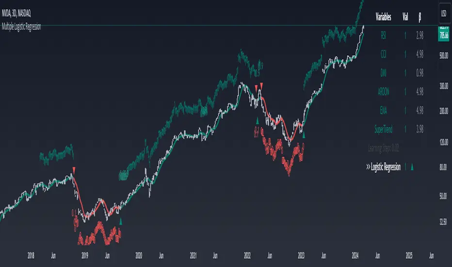
Machine Learning: Multiple Logistic Regression
Multiple Logistic Regression Indicator
The Logistic Regression Indicator for TradingView is a versatile tool that employs multiple logistic regression based on various technical indicators to generate potential buy and sell signals. By utilizing key indicators such as RSI, CCI, DMI, Aroon, EMA, and SuperTrend, the indicator aims to provide a systematic approach to decision-making in financial markets.
How It Works:
Technical Indicators:
The script uses multiple technical indicators such as RSI, CCI, DMI, Aroon, EMA, and SuperTrend as input variables for the logistic regression model.
These indicators are normalized to create categorical variables, providing a consistent scale for the model.
Logistic Regression:
The logistic regression function is applied to the normalized input variables (x1 to x6) with user-defined coefficients (b0 to b6).
The logistic regression model predicts the probability of a binary outcome, with values closer to 1 indicating a bullish signal and values closer to 0 indicating a bearish signal.
Loss Function (Cross-Entropy Loss):
The cross-entropy loss function is calculated to quantify the difference between the predicted probability and the actual outcome.
The goal is to minimize this loss, which essentially measures the model's accuracy.
// Error Function (cross-entropy loss)
loss(y, p) =>
-y * math.log(p) - (1 - y) * math.log(1 - p)
// y - depended variable
// p - multiple logistic regression
Gradient Descent:
Gradient descent is an optimization algorithm used to minimize the loss function by adjusting the weights of the logistic regression model.
The script iteratively updates the weights (b1 to b6) based on the negative gradient of the loss function with respect to each weight.
// Adjusting model weights using gradient descent
b1 -= lr * (p + loss) * x1
b2 -= lr * (p + loss) * x2
b3 -= lr * (p + loss) * x3
b4 -= lr * (p + loss) * x4
b5 -= lr * (p + loss) * x5
b6 -= lr * (p + loss) * x6
// lr - learning rate or step of learning
// p - multiple logistic regression
// x_n - variables
Learning Rate:
The learning rate (lr) determines the step size in the weight adjustment process. It prevents the algorithm from overshooting the minimum of the loss function.
Users can set the learning rate to control the speed and stability of the optimization process.
Visualization:
The script visualizes the output of the logistic regression model by coloring the SMA.
Arrows are plotted at crossover and crossunder points, indicating potential buy and sell signals.
Lables are showing logistic regression values from 1 to 0 above and below bars
Table Display:
A table is displayed on the chart, providing real-time information about the input variables, their values, and the learned coefficients.
This allows traders to monitor the model's interpretation of the technical indicators and observe how the coefficients change over time.
How to Use:
Parameter Adjustment:
Users can adjust the length of technical indicators (rsi_length, cci_length, etc.) and the Z score length based on their preference and market characteristics.
Set the initial values for the regression coefficients (b0 to b6) and the learning rate (lr) according to your trading strategy.
Signal Interpretation:
Buy signals are indicated by an upward arrow (▲), and sell signals are indicated by a downward arrow (▼).
The color-coded SMA provides a visual representation of the logistic regression output by color.
Table Information:
Monitor the table for real-time information on the input variables, their values, and the learned coefficients.
Keep an eye on the learning rate to ensure a balance between model adjustment speed and stability.
Backtesting and Validation:
Before using the script in live trading, conduct thorough backtesting to evaluate its performance under different market conditions.
Validate the model against historical data to ensure its reliability.
KDJ / Connectable [Azullian]Enhance your analysis with our KDJ. Oscillate through buying and selling signals seamlessly, identifying potential reversals with accuracy.
This connectable KDJ indicator is part of an indicator system designed to help test, visualize and build strategy configurations without coding. Like all connectable indicators , it interacts through the TradingView input source, which serves as a signal connector to link indicators to each other. All connectable indicators send signal weight to the next node in the system until it reaches either a connectable signal monitor, signal filter and/or strategy.
█ UNIFORM SETTINGS AND A WAY OF WORK
Although connectable indicators may have specific weight scoring conditions, they all aim to follow a standardized general approach to weight scoring settings, as outlined below.
■ Connectable indicators - Settings
• 🗲 Energy: Energy applies an ATR multiplier to the plotted shapes on the chart. A higher value plots shapes farther away from the candle, enhancing visibility.
• ☼ Brightness: Brightness determines the opacity of the shape plotted on the chart, aiding visibility. Indicator weight also influences opacity.
• → Input: Use the input setting to specify a data source for the indicator. Here you can connect the indicator to other indicators.
• ⌥ Flow: Determine where you want to receive signals from:
○ Both: Weights from this indicator and the connected indicator will apply
○ Indicator only: Only weights from this indicator will apply
○ Input only: Only weights from the connected indicator will apply
• ⥅ Weight multiplier: Multiply all weights in the entire indicator by a given factor, useful for quickly testing different indicators in a granular setup.
• ⥇ Threshold: Set a threshold to indicate the minimum amount of weight it should receive to pass it through to the next indicator.
• ⥱ Limiter: Set a hard limit to the maximum amount of weight that can be fed through the indicator.
■ Connectable indicators - Weight scoring settings
▢ Weight scoring conditions
• SM – Signal mode: Enable specific conditions for weight scoring
○ All: All signals will be scored.
○ Entries only: Only entries will score.
○ Exits only: Only exits will score.
○ Entries & exits: Both entries and exits will score.
○ Zone: Continuous scoring for each candle within the zone.
• SP – Signal period: Defines a range of candles within which a signal can score.
• SC - Signal count: Specifies the number of bars to retrospectively examine and score.
○ Single: Score for a single occurrence
○ All occurrences: Score for all occurrences
○ Single + Threshold: Score for single occurrences within the signal period (SP)
○ Every + Threshold: Score for all occurrences within the signal period (SP)
▢ Weight scoring direction
• ES: Enter Short weight
• XL: Exit long weight
• EL: Enter Long weight
• XS: Exit Short weight
▢ Weight scoring values
• Weights can hold either positive or negative scores. Positive weights enhance a particular trading direction, while negative weights diminish it.
█ KDJ - INDICATOR SETTINGS
■ Main settings
• Enable/Disable Indicator: Toggle the entire indicator on or off.
• S - Source: Choose an alternative data source for the KDJ calculation.
• T - Timeframe: Select an alternative timeframe for the KDJ calculation.
• P - Period: Define the number of bars or periods used in the KDJ calculation.
• SL - Signal line: Adjust the smoothing factor for the KDJ's J line. This not only offers clearer buy/sell cues by reducing market noise but also determines the precise points for potential crossovers and crossunders.
■ Scoring functionality
• The KDJ scores long entries when the J line crosses over the signal (SL) line.
• The KDJ scores long exits when the J line crosses under the signal (SL) line after a prior crossover.
• The KDJ scores long zones the entire time the J line is above the signal (SL) line.
• The KDJ scores short entries when the J line crosses under the signal (SL) line.
• The KDJ scores short exits when the J line crosses over the signal (SL) line after a prior crossunder.
• The KDJ scores short zones the entire time the J line is below the signal (SL) line.
█ PLOTTING
• Standard: Symbols (EL, XS, ES, XL) appear relative to candles based on set conditions. Their opacity and position vary with weight.
• Conditional Settings: A larger icon appears if global conditions are met. For instance, with a Threshold(⥇) of 12, Signal Period (SP) of 3, and Scoring Condition (SC) set to "EVERY", an KDJ signaling over two times in 3 candles (scoring 6 each) triggers a larger icon.
█ USAGE OF CONNECTABLE INDICATORS
■ Connectable chaining mechanism
Connectable indicators can be connected directly to the signal monitor, signal filter or strategy , or they can be daisy chained to each other while the last indicator in the chain connects to the signal monitor, signal filter or strategy. When using a signal filter you can chain the filter to the strategy input to make your chain complete.
• Direct chaining: Connect an indicator directly to the signal monitor, signal filter or strategy through the provided inputs (→).
• Daisy chaining: Connect indicators using the indicator input (→). The first in a daisy chain should have a flow (⌥) set to 'Indicator only'. Subsequent indicators use 'Both' to pass the previous weight. The final indicator connects to the signal monitor, signal filter, or strategy.
■ Set up this indicator with a signal filter and strategy
The indicator provides visual cues based on signal conditions. However, its weight system is best utilized when paired with a connectable signal filter, signal monitor, or strategy .
Let's connect the KDJ to a connectable signal filter and a strategy :
1. Load all relevant indicators
• Load KDJ / Connectable
• Load Signal filter / Connectable
• Load Strategy / Connectable
2. Signal Filter: Connect the KDJ to the Signal Filter
• Open the signal filter settings
• Choose one of the three input dropdowns (1→, 2→, 3→) and choose : KDJ / Connectable: Signal Connector
• Toggle the enable box before the connected input to enable the incoming signal
3. Signal Filter: Update the filter signals settings if needed
• The default settings of the filter enable EL (Enter Long), XL (Exit Long), ES (Enter Short) and XS (Exit Short).
4. Signal Filter: Update the weight threshold settings if needed
• All connectable indicators load by default with a score of 6 for each direction (EL, XL, ES, XS)
• By default, weight threshold (TH) is set at 5. This allows each occurrence to score, as the default score in each connectable indicator is 1 point above the threshold. Adjust to your liking.
5. Strategy: Connect the strategy to the signal filter in the strategy settings
• Select a strategy input → and select the Signal filter: Signal connector
6. Strategy: Enable filter compatible directions
• Set the signal mode of the strategy to a compatible direction with the signal filter.
Now that everything is connected, you'll notice green spikes in the signal filter representing long signals, and red spikes indicating short signals. Trades will also appear on the chart, complemented by a performance overview. Your journey is just beginning: delve into different scoring mechanisms, merge diverse connectable indicators, and craft unique chains. Instantly test your results and discover the potential of your configurations. Dive deep and enjoy the process!
█ BENEFITS
• Adaptable Modular Design: Arrange indicators in diverse structures via direct or daisy chaining, allowing tailored configurations to align with your analysis approach.
• Streamlined Backtesting: Simplify the iterative process of testing and adjusting combinations, facilitating a smoother exploration of potential setups.
• Intuitive Interface: Navigate TradingView with added ease. Integrate desired indicators, adjust settings, and establish alerts without delving into complex code.
• Signal Weight Precision: Leverage granular weight allocation among signals, offering a deeper layer of customization in strategy formulation.
• Advanced Signal Filtering: Define entry and exit conditions with more clarity, granting an added layer of strategy precision.
• Clear Visual Feedback: Distinct visual signals and cues enhance the readability of charts, promoting informed decision-making.
• Standardized Defaults: Indicators are equipped with universally recognized preset settings, ensuring consistency in initial setups across different types like momentum or volatility.
• Reliability: Our indicators are meticulously developed to prevent repainting. We strictly adhere to TradingView's coding conventions, ensuring our code is both performant and clean.
█ COMPATIBLE INDICATORS
Each indicator that incorporates our open-source 'azLibConnector' library and adheres to our conventions can be effortlessly integrated and used as detailed above.
For clarity and recognition within the TradingView platform, we append the suffix ' / Connectable' to every compatible indicator.
█ COMMON MISTAKES, CLARIFICATIONS AND TIPS
• Removing an indicator from a chain: Deleting a linked indicator and confirming the "remove study tree" alert will also remove all underlying indicators in the object tree. Before removing one, disconnect the adjacent indicators and move it to the object stack's bottom.
• Point systems: The azLibConnector provides 500 points for each direction (EL: Enter long, XL: Exit long, ES: Enter short, XS: Exit short) Remember this cap when devising a point structure.
• Flow misconfiguration: In daisy chains the first indicator should always have a flow (⌥) setting of 'indicator only' while other indicator should have a flow (⌥) setting of 'both'.
• Hide attributes: As connectable indicators send through quite some information you'll notice all the arguments are taking up some screenwidth and cause some visual clutter. You can disable arguments in Chart Settings / Status line.
• Layout and abbreviations: To maintain a consistent structure, we use abbreviations for each input. While this may initially seem complex, you'll quickly become familiar with them. Each abbreviation is also explained in the inline tooltips.
• Inputs: Connecting a connectable indicator directly to the strategy delivers the raw signal without a weight threshold, meaning every signal will trigger a trade.
█ A NOTE OF GRATITUDE
Through years of exploring TradingView and Pine Script, we've drawn immense inspiration from the community's knowledge and innovation. Thank you for being a constant source of motivation and insight.
█ RISK DISCLAIMER
Azullian's content, tools, scripts, articles, and educational offerings are presented purely for educational and informational uses. Please be aware that past performance should not be considered a predictor of future results.

Geometric Trend Angle [AstroHub]This script, "Geometric Trend Angle," is designed to identify trend reversals based on the geometric angle of the price chart. Here's a detailed explanation of its originality, functionality, and usage:
Originality and Usefulness:
The uniqueness of this script lies in its approach to trend reversal detection through the calculation of the geometric trend angle. Unlike traditional methods, this script combines the analysis of the angle of the price movement with specific conditions for identifying potential trend reversals.
How it Works:
Length and Trend Angle: The user sets the "Length" parameter, determining the period for calculating the trend angle. The script then computes the trend angle, representing the change in prices over the specified period.
Trend Reversal: The script identifies potential trend reversals when the trend angle changes from positive to negative, and the current closing price is higher than the previous closing price.
Green Reversal: Additionally, the script looks for instances where the trend angle changes from negative to positive, and the current closing price is lower than the previous closing price, indicating a potential reversal to the downside.
Graphical Representation: The script visually highlights the identified reversal points on the chart with labels ("Trend Reversal" and "Green Reversal") and draws a line from the reversal point for better visualization.
Alerts: Traders are alerted to potential trend reversals and green reversals, allowing for timely responses to changing market dynamics.
How to Use:
Apply the script to your TradingView chart.
Customize the "Length" parameter based on your preference and analysis.
Observe the colored candles and graphical elements to identify potential trend reversals.
Pay attention to alerts for timely notifications of reversal signals.
Conclusion:
The "Geometric Trend Angle" script provides a unique perspective on trend reversals, combining geometric angle analysis with specific conditions for improved accuracy. Traders can use it as part of their overall analysis to make informed decisions in the dynamic market environment.
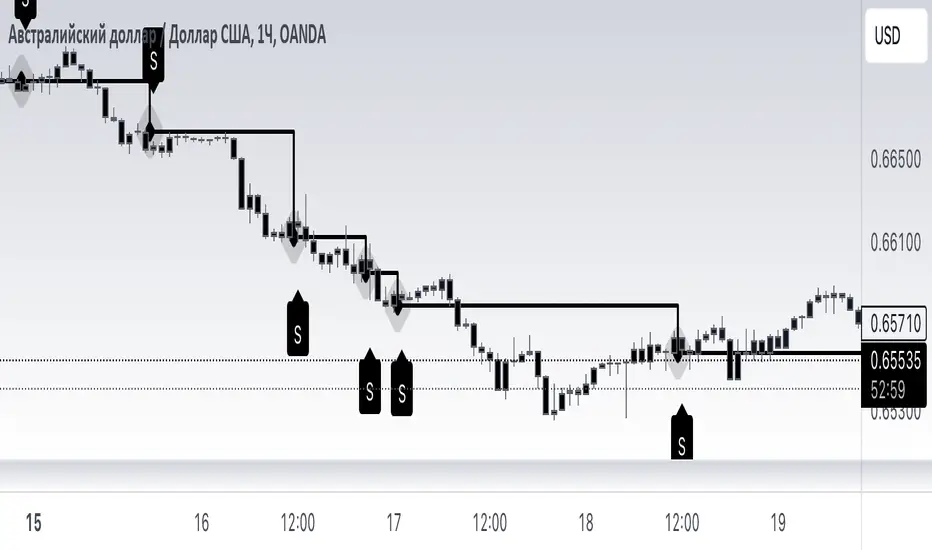
SHIBO V6.0**SHIBO v6 - Fibonacci Impulse Analysis Indicator**
*By Shahab Sadeghi (@shahabs2004)*
**Overview:**
Welcome to SHIBO v6, a revolutionary Fibonacci Impulse Analysis Indicator designed to harness the power of a unique chart pattern. The script employs a reverse Fibonacci methodology to identify powerful impulses that first reach Fibonacci level 0.382, experience a correction, and then continue toward Fibonacci level 1. This description delves into the intricacies of how the script calculates precise price targets based on this distinctive pattern.
keep in mind that this Indicator is based on this Idea that each Impulse have its own support and Resistant Levels(stop loss and Target)
**Key Features:**
1. **Reverse Fibonacci Calculation:** SHIBO v6 introduces a novel approach to Fibonacci analysis. Instead of the conventional method where price targets are set from Fibonacci 0 to 1, this script calculates the distance price moves towards Fibonacci 1 from 0.382. This innovative technique identifies potential reversal and continuation zones with unparalleled accuracy.
2. **Impulse and Correction Identification:** Users play a pivotal role in recognizing high-probability trading opportunities. The script requires manual selection and marking of powerful impulses, focusing on identifying corrections and anticipating potential reversal zones within these impulses.
3. **Optimized Fibonacci Levels:** Leveraging the reverse Fibonacci approach, the script dynamically computes and draws Fibonacci retracement levels (R1, R2, R3) based on the calculated distance the price has moved towards Fibonacci 1. These levels serve as strategic benchmarks, offering insights into potential price movements and areas of interest.
4. **Dynamic Line Drawings:** SHIBO v6 features dynamic line drawings, including impulse start and end points, Fibonacci levels, and stop-loss levels. These visual elements facilitate a comprehensive understanding of the analysis, assisting users in making well-informed trading decisions.
5. **Informative Table Display:** A dedicated table provides crucial information, including impulse start and end points, Fibonacci levels, and percentage deviations from the current price. This table enhances the user's grasp of the analyzed data, fostering effective decision-making.
6. **Prefix Identification:** Users employing multiple SHIBO indicators on a chart can use the Prefix input to assign a unique identifier to each instance. This streamlines the analysis process, particularly when dealing with multiple instances of the indicator.
**How the Script Calculates Targets:**
1. **Impulse Recognition:** Users manually identify a robust impulse in the price movement, signifying a potential trend change or continuation.
2. **Correction Confirmation:** Anticipate or confirm the start of a correction phase within the selected impulse. Corrections often occur after a strong price movement.
3. **Manual Setting of IS and IE Points:** Set the impulse start (IS) and end (IE) points manually based on the identified impulse and correction.
4. **Fibonacci Level Calculation:** The script dynamically calculates Fibonacci levels (R1, R2, R3) based on the distance the price has moved towards Fibonacci 1 from 0.382. These levels serve as potential targets and areas of interest.
5. **Visual Representation:** The script visually represents the calculated levels through dynamic line drawings, providing a clear picture of potential reversal and continuation zones.
**Advanced Usage (Pro Users):**
- **Customizable Line Drawings:** Explore the commented-out lines in the script for additional functionalities and customization options for line drawings. Pro users can tailor the script to align with unique trading strategies.
**Disclaimer:**
Trading carries inherent risks, and SHIBO v6 introduces a distinctive approach to technical analysis. Exercise caution, conduct thorough analysis, and consider risk management strategies before making trading decisions. Past performance does not guarantee future results.
**Support and Feedback:**
Join the community of traders committed to refining strategies based on reverse Fibonacci impulse analysis. Share your experiences, insights, and suggestions to contribute to the continuous improvement of SHIBO v6.
**how Calculations Goes ?**
Imagine you're analyzing a stock price:
IS (Initial Start Price): Let's say the stock price starts at $100.
IE (Initial End Price): After a significant movement, the price reaches $120.
1. Identify Fibonacci Retracement Levels:
fi1 (0.382): This level suggests a potential retracement of 38.2% of the upward move.
fi2 (0.5000): This level represents a 50% retracement, or halfway back to the starting price.
fi3 (0.6180): This level represents the "Golden Ratio" and another potential support/resistance area.
fi4 (0.7860): This level suggests a retracement of 78.6% and can also be used for stop-loss calculations.
2. Calculate Multiples:
m1: Divide the final price ($120) by the starting price ($100) raised to the power of fi1 (120 / 100^0.382). This gives you a value we'll use later.
m2: Similar calculation, but using fi2 instead of fi1.
m3: Similar calculation, but using fi3 instead of fi1.
3. Calculate Target Prices:
Take Profit (Resistance)
TP1: Raise the value of m1 to the power of 1/(1-fi1). This gives you a potential upside target price based on the 38.2% retracement level.
TP2: Similar calculation, but using m2 and fi2.
TP3: Similar calculation, but using m3 and fi3.
4. Calculate Stop-Loss Levels:
Stop loss(Support)
SL1 or Support: Multiply TP1 by the starting price ($100) raised to the power of fi4. This gives you a potential downside stop-loss level based on the 78.6% retracement from TP1.
SL2: Similar calculation, but using TP2 and fi4.
SL3: Similar calculation, but using TP3 and fi4.
5. Calculate Midpoint Level:
MID: Multiply TP1 by the starting price ($100) raised to the power of fi3. This gives you a potential support/resistance level halfway between TP1 and the starting price.
Remember, these are just potential levels and not guaranteed. It's important to use other technical and fundamental analysis alongside Fibonacci retracements.
Here's the breakdown of the steps and their results:
1. Fibonacci levels define potential support and resistance areas:
The chosen Fibonacci levels (0.382, 0.5, 0.618, and 0.786) are often seen as potential zones where the price might stall or reverse after a strong move.
2. Multiples and target prices:
The multiples (m1, m2, m3) represent price ratios based on different retracement levels.
Target prices (TP1, TP2, TP3) are calculated by raising these multiples to specific exponents. These prices suggest areas where the price might encounter resistance after a retracement (not guaranteed predictions).
3. Stop-loss levels:
Stop-loss levels (SL1, SL2, SL3) are based on the target prices and another Fibonacci level (0.786). They mark price points where a trader might exit a trade to manage risk if the price moves against them.
Essentially, the calculations translate Fibonacci retracement levels into concrete price points for potential entry (targets) and exit (stop-loss) points.
*Happy Trading and Empowered Analysis!*
Double Tops/Bottoms [UAlgo]🔶Description:
The "Double Tops/Bottoms " indicator is designed to identify potential double tops and double bottoms on price charts. These patterns are often considered significant as they may indicate a reversal in the prevailing trend. The indicator can be applied to both high/low and close price data, offering flexibility in analyzing different aspects of market behavior.
🔶Key Features:
Source Selection: Users can choose between using high/low or close prices as the basis for identifying double tops and bottoms, allowing for tailored analysis based on specific price actions.
Lookback Length: The indicator offers a customizable lookback length, enabling users to adjust the sensitivity of pattern detection according to their trading preferences and timeframes.
Pivot Length: Users can specify the length of the pivot used in identifying double tops and bottoms, providing flexibility in capturing different market dynamics.
Minimum Bar Count Between Tops/Bottoms: A minimum bar count parameter allows users to control the distance between consecutive tops or bottoms, enhancing the accuracy of pattern recognition.
Pivot Tops/Bottoms Only: The indicator offers the option to focus exclusively on pivot tops and bottoms, streamlining the analysis process for users interested specifically in these key reversal points.
Disclaimer:
Trading involves substantial risk and is not suitable for every investor. The indicator provided here is intended for informational purposes only and should not be construed as investment advice or a recommendation to buy, sell, or hold any securities. Users are solely responsible for evaluating their own investment decisions and should seek professional financial advice if needed. The creator of this indicator (UAlgo) does not guarantee the accuracy, completeness, or reliability of the information provided, and shall not be liable for any losses incurred in connection with its use. By using this indicator, users acknowledge and agree to assume all risks associated with trading activities.

RSI Divergence AlertsIndicator Description: RSI Divergence Alerts
The RSI Divergence indicator is a technical analysis tool that identifies divergences between the Relative Strength Index (RSI) and the price of an asset. The RSI is a momentum indicator that measures the speed and magnitude of recent changes in an asset's price, while divergences occur when there is a disparity between price movements and the RSI.
Indicator Customization:
Overbought and Oversold: The indicator allows you to customize the overbought and oversold levels of the RSI. This allows traders to adjust parameters according to their preferences and the historical behavior of the asset in question.
Indicator Settings and Recommended Adjustments:
Max Bar Distance: This parameter determines the maximum distance allowed between two low or high points for a divergence to be recognized. A higher value may result in more signals, but may also increase the number of false signals. It is recommended to adjust this value based on the volatility of the asset and the time period in which it is being traded.
RSI Length: This is the time period used to calculate the RSI. A longer period smoothes the indicator, while a shorter period makes it more sensitive to price changes. The default value is 14, but traders can adjust it based on their trading strategy and the asset's volatility.
RSI Overbought and Oversold: These values determine the levels at which the RSI is considered overbought and oversold, respectively. The default value for overbought is 75 and for oversold is 35. Traders can adjust these values according to the asset's volatility and its historical analysis. For example, in more volatile assets, it may be useful to use more extreme levels, such as 80 for overbought and 20 for oversold.
When adjusting indicator settings, traders must consider the balance between sensitivity and accuracy. Careful tuning of these parameters can help filter out false signals and identify more reliable trading opportunities.
The alerts functionality in this RSI Divergence indicator is designed to notify traders when a bearish divergence or a bullish divergence is detected. Here's how it works:
Conditionally Triggered Alerts:
Alerts are triggered based on the boolean variables bearishDivergence and bullishDivergence.
If bearishDivergence is true, it indicates that a bearish divergence has been detected.
If bullishDivergence is true, it indicates that a bullish divergence has been detected.
Alert Message:
When a divergence is detected, an alert message is generated to inform the trader about the event.
The message includes details about the divergence, such as the difference in the RSI value between the two points forming the divergence.
For example, for a bearish divergence, the message will include the phrase "Bearish RSI Divergence Detected" and the RSI difference between the high and low points of the divergence.
Alert Frequency:
Alerts are configured to be triggered once per bar close (alert.freq_once_per_bar_close), which means the alert will only be sent once at the close of each bar.
This helps to avoid multiple alerts for the same divergence during the same time period.
Additional Alert Conditions:
In addition to conditionally triggered alert messages, alert conditions are defined for both bearish and bullish divergences.
These alert conditions are useful for configuring custom alerts on trading platforms that support running Pine Script code.
Overall, this alert functionality allows traders to stay informed about potential trading opportunities based on divergences detected by the indicator. This can help traders make faster and more informed decisions in their trading processes.

AI SuperTrend x Pivot Percentile - Strategy [PresentTrading]█ Introduction and How it is Different
The AI SuperTrend x Pivot Percentile strategy is a sophisticated trading approach that integrates AI-driven analysis with traditional technical indicators. Combining the AI SuperTrend with the Pivot Percentile strategy highlights several key advantages:
1. Enhanced Accuracy in Trend Prediction: The AI SuperTrend utilizes K-Nearest Neighbors (KNN) algorithm for trend prediction, improving accuracy by considering historical data patterns. This is complemented by the Pivot Percentile analysis which provides additional context on trend strength.
2. Comprehensive Market Analysis: The integration offers a multi-faceted approach to market analysis, combining AI insights with traditional technical indicators. This dual approach captures a broader range of market dynamics.
BTC 6H L/S Performance
Local
█ Strategy: How it Works - Detailed Explanation
🔶 AI-Enhanced SuperTrend Indicators
1. SuperTrend Calculation:
- The SuperTrend indicator is calculated using a moving average and the Average True Range (ATR). The basic formula is:
- Upper Band = Moving Average + (Multiplier × ATR)
- Lower Band = Moving Average - (Multiplier × ATR)
- The moving average type (SMA, EMA, WMA, RMA, VWMA) and the length of the moving average and ATR are adjustable parameters.
- The direction of the trend is determined based on the position of the closing price in relation to these bands.
2. AI Integration with K-Nearest Neighbors (KNN):
- The KNN algorithm is applied to predict trend direction. It uses historical price data and SuperTrend values to classify the current trend as bullish or bearish.
- The algorithm calculates the 'distance' between the current data point and historical points. The 'k' nearest data points (neighbors) are identified based on this distance.
- A weighted average of these neighbors' trends (bullish or bearish) is calculated to predict the current trend.
For more please check: Multi-TF AI SuperTrend with ADX - Strategy
🔶 Pivot Percentile Analysis
1. Percentile Calculation:
- This involves calculating the percentile ranks for high and low prices over a set of predefined lengths.
- The percentile function is typically defined as:
- Percentile = Value at (P/100) × (N + 1)th position
- Where P is the desired percentile, and N is the number of data points.
2. Trend Strength Evaluation:
- The calculated percentiles for highs and lows are used to determine the strength of bullish and bearish trends.
- For instance, a high percentile rank in the high prices may indicate a strong bullish trend, and vice versa for bearish trends.
For more please check: Pivot Percentile Trend - Strategy
🔶 Strategy Integration
1. Combining SuperTrend and Pivot Percentile:
- The strategy synthesizes the insights from both AI-enhanced SuperTrend and Pivot Percentile analysis.
- It compares the trend direction indicated by the SuperTrend with the strength of the trend as suggested by the Pivot Percentile analysis.
2. Signal Generation:
- A trading signal is generated when both the AI-enhanced SuperTrend and the Pivot Percentile analysis agree on the trend direction.
- For instance, a bullish signal is generated when both the SuperTrend is bullish, and the Pivot Percentile analysis shows strength in bullish trends.
🔶 Risk Management and Filters
- ADX and DMI Filter: The strategy uses the Average Directional Index (ADX) and the Directional Movement Index (DMI) as filters to assess the trend's strength and direction.
- Dynamic Trailing Stop Loss: Based on the SuperTrend indicator, the strategy dynamically adjusts stop-loss levels to manage risk effectively.
This strategy stands out for its ability to combine real-time AI analysis with established technical indicators, offering traders a nuanced and responsive tool for navigating complex market conditions. The equations and algorithms involved are pivotal in accurately identifying market trends and potential trade opportunities.
█ Usage
To effectively use this strategy, traders should:
1. Understand the AI and Pivot Percentile Indicators: A clear grasp of how these indicators work will enable traders to make informed decisions.
2. Interpret the Signals Accurately: The strategy provides bullish, bearish, and neutral signals. Traders should align these signals with their market analysis and trading goals.
3. Monitor Market Conditions: Given that this strategy is sensitive to market dynamics, continuous monitoring is crucial for timely decision-making.
4. Adjust Settings as Needed: Traders should feel free to tweak the input parameters to suit their trading preferences and to respond to changing market conditions.
█Default Settings and Their Impact on Performance
1. Trading Direction (Default: "Both")
Effect: Determines whether the strategy will take long positions, short positions, or both. Adjusting this setting can align the strategy with the trader's market outlook or risk preference.
2. AI Settings (Neighbors: 3, Data Points: 24)
Neighbors: The number of nearest neighbors in the KNN algorithm. A higher number might smooth out noise but could miss subtle, recent changes. A lower number makes the model more sensitive to recent data but may increase noise.
Data Points: Defines the amount of historical data considered. More data points provide a broader context but may dilute recent trends' impact.
3. SuperTrend Settings (Length: 10, Factor: 3.0, MA Source: "WMA")
Length: Affects the sensitivity of the SuperTrend indicator. A longer length results in a smoother, less sensitive indicator, ideal for long-term trends.
Factor: Determines the bandwidth of the SuperTrend. A higher factor creates wider bands, capturing larger price movements but potentially missing short-term signals.
MA Source: The type of moving average used (e.g., WMA - Weighted Moving Average). Different MA types can affect the trend indicator's responsiveness and smoothness.
4. AI Trend Prediction Settings (Price Trend: 10, Prediction Trend: 80)
Price Trend and Prediction Trend Lengths: These settings define the lengths of weighted moving averages for price and SuperTrend, impacting the responsiveness and smoothness of the AI's trend predictions.
5. Pivot Percentile Settings (Length: 10)
Length: Influences the calculation of pivot percentiles. A shorter length makes the percentile more responsive to recent price changes, while a longer length offers a broader view of price trends.
6. ADX and DMI Settings (ADX Length: 14, Time Frame: 'D')
ADX Length: Defines the period for the Average Directional Index calculation. A longer period results in a smoother ADX line.
Time Frame: Sets the time frame for the ADX and DMI calculations, affecting the sensitivity to market changes.
7. Commission, Slippage, and Initial Capital
These settings relate to transaction costs and initial investment, directly impacting net profitability and strategy feasibility.

Dynamic Support/Resistance Zones [ChartPrime]Dynamic Support/Resistance Zones is a new way to visualize key support and resistance levels by analyzing pivot points. It aggregates these points into bins and uses different scoring methods to determine the strength of the zone. The Linear method treats every pivot the same, Time gives more importance to recent pivots, and Volume scores pivots based on trading activity.
It visually represents the strength of price zones using either a visual distribution or an overlay of colors. Areas with many aggregated pivots are marked using the High Color, indicating strong support or resistance. Fewer pivots are shown in Low Color, suggesting weaker levels. Users can also see the score using the distribution mode to more accurately determine the strength of these areas.
The indicator also includes a special moving average line, calculated from pivot prices and their weights. This gives a central pivot level, allowing you to see the average pivot position. We have also provided some smoothing for this line to make it easer to use.
We have included various options to tailor your analysis. These include selecting the scoring method for pivots and adjusting the number of pivots to consider, along with many visual aids. Traders can also set the level of filtering for the distribution of pivots. By default the filter isn't enabled but when it is enabled it allows for a less noisy experience at the expense of precision.
We have included four pivot periods that you can modify and toggle. The idea is that longer period pivots will enhance the strength of the shorter period ones providing a natural way to weight pivot levels. You can also specify whether you want to use pivot high, pivot low, or both in your analysis.
Here are some details on the key inputs:
Weighting Style: Choose how to score pivot points. Options include: Linear: Treats each pivot equally. Time: Gives more importance to recent pivots. Volume: Scores pivots based on trading volume.
Number of Pivots: Set the number of pivots to consider in the calculation. Both pivot highs and lows are treated separately.
Filtering: Adjust the level of filtering applied to the distribution of pivots. A higher value smooths the distribution, providing a cleaner visual representation at the cost of some precision. This setting is crucial for managing the trade-off between clarity and detail in the visualization of support and resistance zones.
Distribution Scale: Determines the scale of the distribution on the screen. It influences both the visual aspect and the precision of the calculations, allowing for a balance between visibility and analytical accuracy.
Manual Precision: Manually set the number of divisions within the range. This setting offers control over the granularity.
Auto Precision: When enabled, it automatically adjusts the precision based on the average range of a candle, ensuring a minimum level of detail in the visualization.
Show Distribution: Toggle the visibility of the distribution of pivot points. When activated, it provides a detailed visual representation of where pivots are concentrated.
Show Score in Distribution: Opt to display the actual score within the distribution. This feature adds a quantitative element to the visual representation, offering a clearer understanding of the pivot point concentration.
Distribution Overlay: Activate a heat map overlay to visualize the distribution of pivots. You can also adjusting the transparency of this overlay, providing a balanced view that does not obstruct the underlying price chart.
Show Support/Resistance: Enable lines that indicate identified support and resistance levels based on the aggregated pivots. This feature provides a clear, actionable insight directly on the chart.
S/R Zone Visibility: Choose to display the support/resistance zones and set their transparency. It offers an extended visual cue about the potential breadth of support or resistance areas.
Pivot Level Average: Introduce a moving average line that's calculated based on the weighted pivot levels. You can also adjust the smoothness of this line.
Dynamic Support/Resistance Zones is an intuitive and versatile trading indicator that offers a novel approach to identifying support and resistance levels by analyzing pivot points. It blends a variety of scoring methods, customizable visual representations, and a unique moving average line. With its customizable settings for pivot analysis, visual clarity, and precision, it's an nifty tool for traders looking to enhance their decision making with detailed and actionable insights.