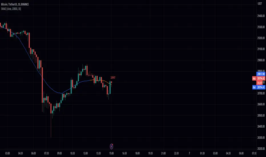
Simple Moving Average Extrapolation via Monte Carlo (SMAE)In this post, I will dive into my Moving Average Extrapolator, a tool that I created to help traders predict future price movements based on past data. I will discuss the underlying logic, its limitations, and the importance of accounting for delays in the moving average. The following code, my Moving Average Extrapolator, will serve as the basis for our discussion.
The Moving Average Extrapolator uses a simple moving average (SMA) to analyze past price movements and make predictions about future price movements. It uses a Monte Carlo simulation to generate possible future price movements based on historical probabilities.
Let's start by understanding the different components of the code:
The movement_probability function calculates the probability of green and red price movements, where green movements indicate an increase in price, and red movements indicate a decrease in price.
The monte function generates an array of potential price movements using a Monte Carlo simulation.
The sim function uses the generated Monte Carlo array to simulate potential future price movements based on the probabilities calculated earlier.
The draw_lines function draws lines connecting the current price to the extrapolated future price movements.
The extrapolate function calculates the extrapolated future price movements based on the provided source, length, and accuracy.
Limitations of My Moving Average Extrapolator:
Reliance on historical data: My Moving Average Extrapolator relies heavily on historical data to make future price predictions. This can be a limitation, as past performance does not guarantee future results. Market conditions can change, making the extrapolator less reliable in predicting future price movements.
Inherent randomness: The Monte Carlo simulation introduces an element of randomness in the extrapolator's predictions. While this can help in exploring various scenarios, it may not always accurately predict future price movements.
Delay in the moving average: Moving averages inherently have a delay, as they are based on past data. This delay can cause my Moving Average Extrapolator to be less accurate in predicting immediate price movements.
Accounting for Delays in the Moving Average:
It is essential to account for the delay in the moving average to improve the accuracy of my Moving Average Extrapolator. I have taken this into account by introducing a delay variable (delay) in the draw_lines function. The delay variable calculates the delay as half the moving average's length and adjusts the time axis accordingly.
This adjustment helps in reducing the lag in the extrapolator's predictions, making it more accurate and useful for traders. However, it is important to note that even with this adjustment, my Moving Average Extrapolator is still subject to the limitations discussed earlier.
Adding Custom Lookback Period to My Moving Average Extrapolator:
To enhance the functionality and adaptability of my Moving Average Extrapolator, I have implemented an option to set a custom lookback period. The lookback period determines how far back in the historical data the Moving Average Extrapolator should start its analysis.
To achieve this, I have included a method to obtain the current bar index and then calculate the starting bar index by subtracting the desired lookback period.
Here's how to implement the custom lookback period in the Moving Average Extrapolator:
Get the current bar index: I use the bar_index built-in variable to get the current bar index, which represents the current position in the historical data.
Set the start index: To set the start index, you can subtract the desired lookback period from the current bar index. In the code, I have defined a user-input number variable, which can be set to the desired lookback period. By default, it is set to 20800. The starting index for the Moving Average Extrapolator's analysis is calculated as bar_index - number.
Here's the relevant code snippet:
number = input.int(20800, "Bar Start")
And to conditionally run the calculations:
if bar_index > number
draw_lines(avg, extrapolate(close, length, 10), length, extrapolate)
By implementing this custom lookback period, users can easily adjust the starting point of the Moving Average Extrapolator based on their preferences and trading strategies. This allows for more flexibility and adaptability to different market scenarios and ensures that the Moving Average Extrapolator remains a valuable tool for traders.
Conclusion:
My Moving Average Extrapolator can be a valuable tool for traders looking to predict future price movements based on historical data. However, it is essential to understand its limitations and the need to account for the delay in the moving average. By considering these factors, traders can make better-informed decisions and use my Moving Average Extrapolator to complement their trading strategies effectively.
Cerca negli script per "accuracy"
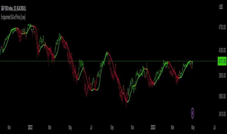
Endpointed SSA of Price [Loxx]The Endpointed SSA of Price: A Comprehensive Tool for Market Analysis and Decision-Making
The financial markets present sophisticated challenges for traders and investors as they navigate the complexities of market behavior. To effectively interpret and capitalize on these complexities, it is crucial to employ powerful analytical tools that can reveal hidden patterns and trends. One such tool is the Endpointed SSA of Price, which combines the strengths of Caterpillar Singular Spectrum Analysis, a sophisticated time series decomposition method, with insights from the fields of economics, artificial intelligence, and machine learning.
The Endpointed SSA of Price has its roots in the interdisciplinary fusion of mathematical techniques, economic understanding, and advancements in artificial intelligence. This unique combination allows for a versatile and reliable tool that can aid traders and investors in making informed decisions based on comprehensive market analysis.
The Endpointed SSA of Price is not only valuable for experienced traders but also serves as a useful resource for those new to the financial markets. By providing a deeper understanding of market forces, this innovative indicator equips users with the knowledge and confidence to better assess risks and opportunities in their financial pursuits.
█ Exploring Caterpillar SSA: Applications in AI, Machine Learning, and Finance
Caterpillar SSA (Singular Spectrum Analysis) is a non-parametric method for time series analysis and signal processing. It is based on a combination of principles from classical time series analysis, multivariate statistics, and the theory of random processes. The method was initially developed in the early 1990s by a group of Russian mathematicians, including Golyandina, Nekrutkin, and Zhigljavsky.
Background Information:
SSA is an advanced technique for decomposing time series data into a sum of interpretable components, such as trend, seasonality, and noise. This decomposition allows for a better understanding of the underlying structure of the data and facilitates forecasting, smoothing, and anomaly detection. Caterpillar SSA is a particular implementation of SSA that has proven to be computationally efficient and effective for handling large datasets.
Uses in AI and Machine Learning:
In recent years, Caterpillar SSA has found applications in various fields of artificial intelligence (AI) and machine learning. Some of these applications include:
1. Feature extraction: Caterpillar SSA can be used to extract meaningful features from time series data, which can then serve as inputs for machine learning models. These features can help improve the performance of various models, such as regression, classification, and clustering algorithms.
2. Dimensionality reduction: Caterpillar SSA can be employed as a dimensionality reduction technique, similar to Principal Component Analysis (PCA). It helps identify the most significant components of a high-dimensional dataset, reducing the computational complexity and mitigating the "curse of dimensionality" in machine learning tasks.
3. Anomaly detection: The decomposition of a time series into interpretable components through Caterpillar SSA can help in identifying unusual patterns or outliers in the data. Machine learning models trained on these decomposed components can detect anomalies more effectively, as the noise component is separated from the signal.
4. Forecasting: Caterpillar SSA has been used in combination with machine learning techniques, such as neural networks, to improve forecasting accuracy. By decomposing a time series into its underlying components, machine learning models can better capture the trends and seasonality in the data, resulting in more accurate predictions.
Application in Financial Markets and Economics:
Caterpillar SSA has been employed in various domains within financial markets and economics. Some notable applications include:
1. Stock price analysis: Caterpillar SSA can be used to analyze and forecast stock prices by decomposing them into trend, seasonal, and noise components. This decomposition can help traders and investors better understand market dynamics, detect potential turning points, and make more informed decisions.
2. Economic indicators: Caterpillar SSA has been used to analyze and forecast economic indicators, such as GDP, inflation, and unemployment rates. By decomposing these time series, researchers can better understand the underlying factors driving economic fluctuations and develop more accurate forecasting models.
3. Portfolio optimization: By applying Caterpillar SSA to financial time series data, portfolio managers can better understand the relationships between different assets and make more informed decisions regarding asset allocation and risk management.
Application in the Indicator:
In the given indicator, Caterpillar SSA is applied to a financial time series (price data) to smooth the series and detect significant trends or turning points. The method is used to decompose the price data into a set number of components, which are then combined to generate a smoothed signal. This signal can help traders and investors identify potential entry and exit points for their trades.
The indicator applies the Caterpillar SSA method by first constructing the trajectory matrix using the price data, then computing the singular value decomposition (SVD) of the matrix, and finally reconstructing the time series using a selected number of components. The reconstructed series serves as a smoothed version of the original price data, highlighting significant trends and turning points. The indicator can be customized by adjusting the lag, number of computations, and number of components used in the reconstruction process. By fine-tuning these parameters, traders and investors can optimize the indicator to better match their specific trading style and risk tolerance.
Caterpillar SSA is versatile and can be applied to various types of financial instruments, such as stocks, bonds, commodities, and currencies. It can also be combined with other technical analysis tools or indicators to create a comprehensive trading system. For example, a trader might use Caterpillar SSA to identify the primary trend in a market and then employ additional indicators, such as moving averages or RSI, to confirm the trend and generate trading signals.
In summary, Caterpillar SSA is a powerful time series analysis technique that has found applications in AI and machine learning, as well as financial markets and economics. By decomposing a time series into interpretable components, Caterpillar SSA enables better understanding of the underlying structure of the data, facilitating forecasting, smoothing, and anomaly detection. In the context of financial trading, the technique is used to analyze price data, detect significant trends or turning points, and inform trading decisions.
█ Input Parameters
This indicator takes several inputs that affect its signal output. These inputs can be classified into three categories: Basic Settings, UI Options, and Computation Parameters.
Source: This input represents the source of price data, which is typically the closing price of an asset. The user can select other price data, such as opening price, high price, or low price. The selected price data is then utilized in the Caterpillar SSA calculation process.
Lag: The lag input determines the window size used for the time series decomposition. A higher lag value implies that the SSA algorithm will consider a longer range of historical data when extracting the underlying trend and components. This parameter is crucial, as it directly impacts the resulting smoothed series and the quality of extracted components.
Number of Computations: This input, denoted as 'ncomp,' specifies the number of eigencomponents to be considered in the reconstruction of the time series. A smaller value results in a smoother output signal, while a higher value retains more details in the series, potentially capturing short-term fluctuations.
SSA Period Normalization: This input is used to normalize the SSA period, which adjusts the significance of each eigencomponent to the overall signal. It helps in making the algorithm adaptive to different timeframes and market conditions.
Number of Bars: This input specifies the number of bars to be processed by the algorithm. It controls the range of data used for calculations and directly affects the computation time and the output signal.
Number of Bars to Render: This input sets the number of bars to be plotted on the chart. A higher value slows down the computation but provides a more comprehensive view of the indicator's performance over a longer period. This value controls how far back the indicator is rendered.
Color bars: This boolean input determines whether the bars should be colored according to the signal's direction. If set to true, the bars are colored using the defined colors, which visually indicate the trend direction.
Show signals: This boolean input controls the display of buy and sell signals on the chart. If set to true, the indicator plots shapes (triangles) to represent long and short trade signals.
Static Computation Parameters:
The indicator also includes several internal parameters that affect the Caterpillar SSA algorithm, such as Maxncomp, MaxLag, and MaxArrayLength. These parameters set the maximum allowed values for the number of computations, the lag, and the array length, ensuring that the calculations remain within reasonable limits and do not consume excessive computational resources.
█ A Note on Endpionted, Non-repainting Indicators
An endpointed indicator is one that does not recalculate or repaint its past values based on new incoming data. In other words, the indicator's previous signals remain the same even as new price data is added. This is an important feature because it ensures that the signals generated by the indicator are reliable and accurate, even after the fact.
When an indicator is non-repainting or endpointed, it means that the trader can have confidence in the signals being generated, knowing that they will not change as new data comes in. This allows traders to make informed decisions based on historical signals, without the fear of the signals being invalidated in the future.
In the case of the Endpointed SSA of Price, this non-repainting property is particularly valuable because it allows traders to identify trend changes and reversals with a high degree of accuracy, which can be used to inform trading decisions. This can be especially important in volatile markets where quick decisions need to be made.
Low-lag TrendlineWe apply the LLT trend timing to daily data of market indices such as the Shanghai and Shenzhen 300, Shanghai Composite Index, and Shenzhen Composite Index, and use the tangent method to make direction judgments, obtaining a good risk return situation. Compared to MA trend timing, we found that the LLT model has a shorter timing period and better stability. However, there is a problem with using the tangent method to track trend lines, which is that near the turning point of the trend, the tangent slope is prone to oscillate near zero, resulting in multiple timing judgments and a decrease in accuracy. This is equivalent to embedding a certain stop loss mechanism in the timing model, so we call this type of timing method transactional timing. For the LLT indicator, once the trend is established, holding positions can maintain a relatively long profit period, and although there are many volatile trading times near the inflection point, the holding time is often very short. Therefore, for transactional timing, when the accuracy of judgment is relatively low, the proportion of correct judgment time is often high, and profits mainly come from this part of the contribution.

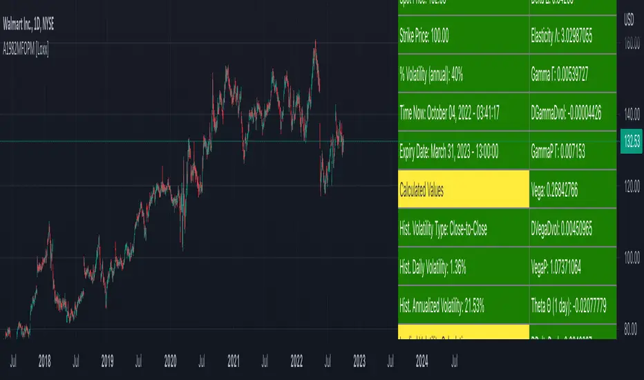
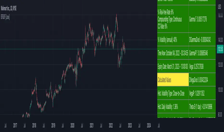
Asay (1982) Margined Futures Option Pricing Model [Loxx]Asay (1982) Margined Futures Option Pricing Model is an adaptation of the Black-Scholes-Merton Option Pricing Model including Analytical Greeks and implied volatility calculations. The following information is an excerpt from Espen Gaarder Haug's book "Option Pricing Formulas". This version is to price Options on Futures where premium is fully margined. This means the Risk-free Rate, dividend, and cost to carry are all zero. The options sensitivities (Greeks) are the partial derivatives of the Black-Scholes-Merton ( BSM ) formula. Analytical Greeks for our purposes here are broken down into various categories:
Delta Greeks: Delta, DDeltaDvol, Elasticity
Gamma Greeks: Gamma, GammaP, DGammaDvol, Speed
Vega Greeks: Vega , DVegaDvol/Vomma, VegaP
Theta Greeks: Theta
Probability Greeks: StrikeDelta, Risk Neutral Density
(See the code for more details)
Black-Scholes-Merton Option Pricing
The Black-Scholes-Merton model can be "generalized" by incorporating a cost-of-carry rate b. This model can be used to price European options on stocks, stocks paying a continuous dividend yield, options on futures , and currency options:
c = S * e^((b - r) * T) * N(d1) - X * e^(-r * T) * N(d2)
p = X * e^(-r * T) * N(-d2) - S * e^((b - r) * T) * N(-d1)
where
d1 = (log(S / X) + (b + v^2 / 2) * T) / (v * T^0.5)
d2 = d1 - v * T^0.5
b = r ... gives the Black and Scholes (1973) stock option model.
b = r — q ... gives the Merton (1973) stock option model with continuous dividend yield q.
b = 0 ... gives the Black (1976) futures option model.
b = 0 and r = 0 ... gives the Asay (1982) margined futures option model. <== this is the one used for this indicator!
b = r — rf ... gives the Garman and Kohlhagen (1983) currency option model.
Inputs
S = Stock price.
X = Strike price of option.
T = Time to expiration in years.
r = Risk-free rate
d = dividend yield
v = Volatility of the underlying asset price
cnd (x) = The cumulative normal distribution function
nd(x) = The standard normal density function
convertingToCCRate(r, cmp ) = Rate compounder
gImpliedVolatilityNR(string CallPutFlag, float S, float x, float T, float r, float b, float cm , float epsilon) = Implied volatility via Newton Raphson
gBlackScholesImpVolBisection(string CallPutFlag, float S, float x, float T, float r, float b, float cm ) = implied volatility via bisection
Implied Volatility: The Bisection Method
The Newton-Raphson method requires knowledge of the partial derivative of the option pricing formula with respect to volatility ( vega ) when searching for the implied volatility . For some options (exotic and American options in particular), vega is not known analytically. The bisection method is an even simpler method to estimate implied volatility when vega is unknown. The bisection method requires two initial volatility estimates (seed values):
1. A "low" estimate of the implied volatility , al, corresponding to an option value, CL
2. A "high" volatility estimate, aH, corresponding to an option value, CH
The option market price, Cm , lies between CL and cH . The bisection estimate is given as the linear interpolation between the two estimates:
v(i + 1) = v(L) + (c(m) - c(L)) * (v(H) - v(L)) / (c(H) - c(L))
Replace v(L) with v(i + 1) if c(v(i + 1)) < c(m), or else replace v(H) with v(i + 1) if c(v(i + 1)) > c(m) until |c(m) - c(v(i + 1))| <= E, at which point v(i + 1) is the implied volatility and E is the desired degree of accuracy.
Implied Volatility: Newton-Raphson Method
The Newton-Raphson method is an efficient way to find the implied volatility of an option contract. It is nothing more than a simple iteration technique for solving one-dimensional nonlinear equations (any introductory textbook in calculus will offer an intuitive explanation). The method seldom uses more than two to three iterations before it converges to the implied volatility . Let
v(i + 1) = v(i) + (c(v(i)) - c(m)) / (dc / dv (i))
until |c(m) - c(v(i + 1))| <= E at which point v(i + 1) is the implied volatility , E is the desired degree of accuracy, c(m) is the market price of the option, and dc/ dv (i) is the vega of the option evaluaated at v(i) (the sensitivity of the option value for a small change in volatility ).
Things to know
Only works on the daily timeframe and for the current source price.
You can adjust the text size to fit the screen
Black-76 Options on Futures [Loxx]Black-76 Options on Futures is an adaptation of the Black-Scholes-Merton Option Pricing Model including Analytical Greeks and implied volatility calculations. The following information is an excerpt from Espen Gaarder Haug's book "Option Pricing Formulas". This version is to price Options on Futures. The options sensitivities (Greeks) are the partial derivatives of the Black-Scholes-Merton ( BSM ) formula. Analytical Greeks for our purposes here are broken down into various categories:
Delta Greeks: Delta, DDeltaDvol, Elasticity
Gamma Greeks: Gamma, GammaP, DGammaDvol, Speed
Vega Greeks: Vega , DVegaDvol/Vomma, VegaP
Theta Greeks: Theta
Rate/Carry Greeks: Rho futures option
Probability Greeks: StrikeDelta, Risk Neutral Density
(See the code for more details)
Black-Scholes-Merton Option Pricing
The Black-Scholes-Merton model can be "generalized" by incorporating a cost-of-carry rate b. This model can be used to price European options on stocks, stocks paying a continuous dividend yield, options on futures , and currency options:
c = S * e^((b - r) * T) * N(d1) - X * e^(-r * T) * N(d2)
p = X * e^(-r * T) * N(-d2) - S * e^((b - r) * T) * N(-d1)
where
d1 = (log(S / X) + (b + v^2 / 2) * T) / (v * T^0.5)
d2 = d1 - v * T^0.5
b = r ... gives the Black and Scholes (1973) stock option model.
b = r — q ... gives the Merton (1973) stock option model with continuous dividend yield q.
b = 0 ... gives the Black (1976) futures option model. <== this is the one used for this indicator!
b = 0 and r = 0 ... gives the Asay (1982) margined futures option model.
b = r — rf ... gives the Garman and Kohlhagen (1983) currency option model.
Inputs
S = Stock price.
X = Strike price of option.
T = Time to expiration in years.
r = Risk-free rate
d = dividend yield
v = Volatility of the underlying asset price
cnd (x) = The cumulative normal distribution function
nd(x) = The standard normal density function
convertingToCCRate(r, cmp ) = Rate compounder
gImpliedVolatilityNR(string CallPutFlag, float S, float x, float T, float r, float b, float cm , float epsilon) = Implied volatility via Newton Raphson
gBlackScholesImpVolBisection(string CallPutFlag, float S, float x, float T, float r, float b, float cm ) = implied volatility via bisection
Implied Volatility: The Bisection Method
The Newton-Raphson method requires knowledge of the partial derivative of the option pricing formula with respect to volatility ( vega ) when searching for the implied volatility . For some options (exotic and American options in particular), vega is not known analytically. The bisection method is an even simpler method to estimate implied volatility when vega is unknown. The bisection method requires two initial volatility estimates (seed values):
1. A "low" estimate of the implied volatility , al, corresponding to an option value, CL
2. A "high" volatility estimate, aH, corresponding to an option value, CH
The option market price, Cm , lies between CL and cH . The bisection estimate is given as the linear interpolation between the two estimates:
v(i + 1) = v(L) + (c(m) - c(L)) * (v(H) - v(L)) / (c(H) - c(L))
Replace v(L) with v(i + 1) if c(v(i + 1)) < c(m), or else replace v(H) with v(i + 1) if c(v(i + 1)) > c(m) until |c(m) - c(v(i + 1))| <= E, at which point v(i + 1) is the implied volatility and E is the desired degree of accuracy.
Implied Volatility: Newton-Raphson Method
The Newton-Raphson method is an efficient way to find the implied volatility of an option contract. It is nothing more than a simple iteration technique for solving one-dimensional nonlinear equations (any introductory textbook in calculus will offer an intuitive explanation). The method seldom uses more than two to three iterations before it converges to the implied volatility . Let
v(i + 1) = v(i) + (c(v(i)) - c(m)) / (dc / dv (i))
until |c(m) - c(v(i + 1))| <= E at which point v(i + 1) is the implied volatility , E is the desired degree of accuracy, c(m) is the market price of the option, and dc/ dv (i) is the vega of the option evaluaated at v(i) (the sensitivity of the option value for a small change in volatility ).
Things to know
Only works on the daily timeframe and for the current source price.
You can adjust the text size to fit the screen
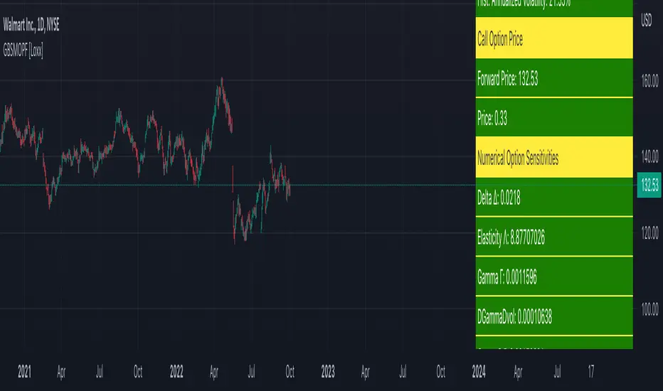
Garman and Kohlhagen (1983) for Currency Options [Loxx]Garman and Kohlhagen (1983) for Currency Options is an adaptation of the Black-Scholes-Merton Option Pricing Model including Analytical Greeks and implied volatility calculations. The following information is an excerpt from Espen Gaarder Haug's book "Option Pricing Formulas". This version of BSMOPM is to price Currency Options. The options sensitivities (Greeks) are the partial derivatives of the Black-Scholes-Merton ( BSM ) formula. Analytical Greeks for our purposes here are broken down into various categories:
Delta Greeks: Delta, DDeltaDvol, Elasticity
Gamma Greeks: Gamma, GammaP, DGammaDSpot/speed, DGammaDvol/Zomma
Vega Greeks: Vega , DVegaDvol/Vomma, VegaP, Speed
Theta Greeks: Theta
Rate/Carry Greeks: Rho, Rho futures option, Carry Rho, Phi/Rho2
Probability Greeks: StrikeDelta, Risk Neutral Density
(See the code for more details)
Black-Scholes-Merton Option Pricing for Currency Options
The Garman and Kohlhagen (1983) modified Black-Scholes model can be used to price European currency options; see also Grabbe (1983). The model is mathematically equivalent to the Merton (1973) model presented earlier. The only difference is that the dividend yield is replaced by the risk-free rate of the foreign currency rf:
c = S * e^(-rf * T) * N(d1) - X * e^(-r * T) * N(d2)
p = X * e^(-r * T) * N(-d2) - S * e^(-rf * T) * N(-d1)
where
d1 = (log(S / X) + (r - rf + v^2 / 2) * T) / (v * T^0.5)
d2 = d1 - v * T^0.5
For more information on currency options, see DeRosa (2000)
Inputs
S = Stock price.
X = Strike price of option.
T = Time to expiration in years.
r = Risk-free rate
rf = Risk-free rate of the foreign currency
v = Volatility of the underlying asset price
cnd (x) = The cumulative normal distribution function
nd(x) = The standard normal density function
convertingToCCRate(r, cmp ) = Rate compounder
gImpliedVolatilityNR(string CallPutFlag, float S, float x, float T, float r, float b, float cm , float epsilon) = Implied volatility via Newton Raphson
gBlackScholesImpVolBisection(string CallPutFlag, float S, float x, float T, float r, float b, float cm ) = implied volatility via bisection
Implied Volatility: The Bisection Method
The Newton-Raphson method requires knowledge of the partial derivative of the option pricing formula with respect to volatility ( vega ) when searching for the implied volatility . For some options (exotic and American options in particular), vega is not known analytically. The bisection method is an even simpler method to estimate implied volatility when vega is unknown. The bisection method requires two initial volatility estimates (seed values):
1. A "low" estimate of the implied volatility , al, corresponding to an option value, CL
2. A "high" volatility estimate, aH, corresponding to an option value, CH
The option market price, Cm , lies between CL and cH . The bisection estimate is given as the linear interpolation between the two estimates:
v(i + 1) = v(L) + (c(m) - c(L)) * (v(H) - v(L)) / (c(H) - c(L))
Replace v(L) with v(i + 1) if c(v(i + 1)) < c(m), or else replace v(H) with v(i + 1) if c(v(i + 1)) > c(m) until |c(m) - c(v(i + 1))| <= E, at which point v(i + 1) is the implied volatility and E is the desired degree of accuracy.
Implied Volatility: Newton-Raphson Method
The Newton-Raphson method is an efficient way to find the implied volatility of an option contract. It is nothing more than a simple iteration technique for solving one-dimensional nonlinear equations (any introductory textbook in calculus will offer an intuitive explanation). The method seldom uses more than two to three iterations before it converges to the implied volatility . Let
v(i + 1) = v(i) + (c(v(i)) - c(m)) / (dc / dv (i))
until |c(m) - c(v(i + 1))| <= E at which point v(i + 1) is the implied volatility , E is the desired degree of accuracy, c(m) is the market price of the option, and dc/ dv (i) is the vega of the option evaluaated at v(i) (the sensitivity of the option value for a small change in volatility ).
Things to know
Only works on the daily timeframe and for the current source price.
You can adjust the text size to fit the screen
Related indicators:
BSM OPM 1973 w/ Continuous Dividend Yield
Black-Scholes 1973 OPM on Non-Dividend Paying Stocks
Generalized Black-Scholes-Merton w/ Analytical Greeks
Generalized Black-Scholes-Merton Option Pricing Formula
Sprenkle 1964 Option Pricing Model w/ Num. Greeks
Modified Bachelier Option Pricing Model w/ Num. Greeks
Bachelier 1900 Option Pricing Model w/ Numerical Greeks

BSM OPM 1973 w/ Continuous Dividend Yield [Loxx]Generalized Black-Scholes-Merton w/ Analytical Greeks is an adaptation of the Black-Scholes-Merton Option Pricing Model including Analytical Greeks and implied volatility calculations. The following information is an excerpt from Espen Gaarder Haug's book "Option Pricing Formulas". The options sensitivities (Greeks) are the partial derivatives of the Black-Scholes-Merton ( BSM ) formula. Analytical Greeks for our purposes here are broken down into various categories:
Delta Greeks: Delta, DDeltaDvol, Elasticity
Gamma Greeks: Gamma, GammaP, DGammaDSpot/speed, DGammaDvol/Zomma
Vega Greeks: Vega , DVegaDvol/Vomma, VegaP
Theta Greeks: Theta
Rate/Carry Greeks: Rho, Rho futures option, Carry Rho, Phi/Rho2
Probability Greeks: StrikeDelta, Risk Neutral Density
(See the code for more details)
Black-Scholes-Merton Option Pricing
The Black-Scholes-Merton model can be "generalized" by incorporating a cost-of-carry rate b. This model can be used to price European options on stocks, stocks paying a continuous dividend yield, options on futures, and currency options:
c = S * e^((b - r) * T) * N(d1) - X * e^(-r * T) * N(d2)
p = X * e^(-r * T) * N(-d2) - S * e^((b - r) * T) * N(-d1)
where
d1 = (log(S / X) + (b + v^2 / 2) * T) / (v * T^0.5)
d2 = d1 - v * T^0.5
b = r ... gives the Black and Scholes (1973) stock option model.
b = r — q ... gives the Merton (1973) stock option model with continuous dividend yield q. <== this is the one used for this indicator!
b = 0 ... gives the Black (1976) futures option model.
b = 0 and r = 0 ... gives the Asay (1982) margined futures option model.
b = r — rf ... gives the Garman and Kohlhagen (1983) currency option model.
Inputs
S = Stock price.
X = Strike price of option.
T = Time to expiration in years.
r = Risk-free rate
d = dividend yield
v = Volatility of the underlying asset price
cnd (x) = The cumulative normal distribution function
nd(x) = The standard normal density function
convertingToCCRate(r, cmp ) = Rate compounder
gImpliedVolatilityNR(string CallPutFlag, float S, float x, float T, float r, float b, float cm , float epsilon) = Implied volatility via Newton Raphson
gBlackScholesImpVolBisection(string CallPutFlag, float S, float x, float T, float r, float b, float cm ) = implied volatility via bisection
Implied Volatility: The Bisection Method
The Newton-Raphson method requires knowledge of the partial derivative of the option pricing formula with respect to volatility ( vega ) when searching for the implied volatility . For some options (exotic and American options in particular), vega is not known analytically. The bisection method is an even simpler method to estimate implied volatility when vega is unknown. The bisection method requires two initial volatility estimates (seed values):
1. A "low" estimate of the implied volatility , al, corresponding to an option value, CL
2. A "high" volatility estimate, aH, corresponding to an option value, CH
The option market price, Cm , lies between CL and cH . The bisection estimate is given as the linear interpolation between the two estimates:
v(i + 1) = v(L) + (c(m) - c(L)) * (v(H) - v(L)) / (c(H) - c(L))
Replace v(L) with v(i + 1) if c(v(i + 1)) < c(m), or else replace v(H) with v(i + 1) if c(v(i + 1)) > c(m) until |c(m) - c(v(i + 1))| <= E, at which point v(i + 1) is the implied volatility and E is the desired degree of accuracy.
Implied Volatility: Newton-Raphson Method
The Newton-Raphson method is an efficient way to find the implied volatility of an option contract. It is nothing more than a simple iteration technique for solving one-dimensional nonlinear equations (any introductory textbook in calculus will offer an intuitive explanation). The method seldom uses more than two to three iterations before it converges to the implied volatility . Let
v(i + 1) = v(i) + (c(v(i)) - c(m)) / (dc / dv (i))
until |c(m) - c(v(i + 1))| <= E at which point v(i + 1) is the implied volatility , E is the desired degree of accuracy, c(m) is the market price of the option, and dc/ dv (i) is the vega of the option evaluaated at v(i) (the sensitivity of the option value for a small change in volatility ).
Things to know
Only works on the daily timeframe and for the current source price.
You can adjust the text size to fit the screen

Black-Scholes 1973 OPM on Non-Dividend Paying Stocks [Loxx]Black-Scholes 1973 OPM on Non-Dividend Paying Stocks is an adaptation of the Black-Scholes-Merton Option Pricing Model including Analytical Greeks and implied volatility calculations. Making b equal to r yields the BSM model where dividends are not considered. The following information is an excerpt from Espen Gaarder Haug's book "Option Pricing Formulas". The options sensitivities (Greeks) are the partial derivatives of the Black-Scholes-Merton ( BSM ) formula. For our purposes here are, Analytical Greeks are broken down into various categories:
Delta Greeks: Delta, DDeltaDvol, Elasticity
Gamma Greeks: Gamma, GammaP, DGammaDSpot/speed, DGammaDvol/Zomma
Vega Greeks: Vega , DVegaDvol/Vomma, VegaP
Theta Greeks: Theta
Rate/Carry Greeks: Rho
Probability Greeks: StrikeDelta, Risk Neutral Density
(See the code for more details)
Black-Scholes-Merton Option Pricing
The BSM formula and its binomial counterpart may easily be the most used "probability model/tool" in everyday use — even if we con- sider all other scientific disciplines. Literally tens of thousands of people, including traders, market makers, and salespeople, use option formulas several times a day. Hardly any other area has seen such dramatic growth as the options and derivatives businesses. In this chapter we look at the various versions of the basic option formula. In 1997 Myron Scholes and Robert Merton were awarded the Nobel Prize (The Bank of Sweden Prize in Economic Sciences in Memory of Alfred Nobel). Unfortunately, Fischer Black died of cancer in 1995 before he also would have received the prize.
It is worth mentioning that it was not the option formula itself that Myron Scholes and Robert Merton were awarded the Nobel Prize for, the formula was actually already invented, but rather for the way they derived it — the replicating portfolio argument, continuous- time dynamic delta hedging, as well as making the formula consistent with the capital asset pricing model (CAPM). The continuous dynamic replication argument is unfortunately far from robust. The popularity among traders for using option formulas heavily relies on hedging options with options and on the top of this dynamic delta hedging, see Higgins (1902), Nelson (1904), Mello and Neuhaus (1998), Derman and Taleb (2005), as well as Haug (2006) for more details on this topic. In any case, this book is about option formulas and not so much about how to derive them.
Provided here are the various versions of the Black-Scholes-Merton formula presented in the literature. All formulas in this section are originally derived based on the underlying asset S follows a geometric Brownian motion
dS = mu * S * dt + v * S * dz
where t is the expected instantaneous rate of return on the underlying asset, a is the instantaneous volatility of the rate of return, and dz is a Wiener process.
The formula derived by Black and Scholes (1973) can be used to value a European option on a stock that does not pay dividends before the option's expiration date. Letting c and p denote the price of European call and put options, respectively, the formula states that
c = S * N(d1) - X * e^(-r * T) * N(d2)
p = X * e^(-r * T) * N(d2) - S * N(d1)
where
d1 = (log(S / X) + (r + v^2 / 2) * T) / (v * T^0.5)
d2 = (log(S / X) + (r - v^2 / 2) * T) / (v * T^0.5) = d1 - v * T^0.5
**This version of the Black-Scholes formula can also be used to price American call options on a non-dividend-paying stock, since it will never be optimal to exercise the option before expiration.**
Inputs
S = Stock price.
X = Strike price of option.
T = Time to expiration in years.
r = Risk-free rate
b = Cost of carry
v = Volatility of the underlying asset price
cnd (x) = The cumulative normal distribution function
nd(x) = The standard normal density function
convertingToCCRate(r, cmp ) = Rate compounder
gImpliedVolatilityNR(string CallPutFlag, float S, float x, float T, float r, float b, float cm , float epsilon) = Implied volatility via Newton Raphson
gBlackScholesImpVolBisection(string CallPutFlag, float S, float x, float T, float r, float b, float cm ) = implied volatility via bisection
Implied Volatility: The Bisection Method
The Newton-Raphson method requires knowledge of the partial derivative of the option pricing formula with respect to volatility ( vega ) when searching for the implied volatility . For some options (exotic and American options in particular), vega is not known analytically. The bisection method is an even simpler method to estimate implied volatility when vega is unknown. The bisection method requires two initial volatility estimates (seed values):
1. A "low" estimate of the implied volatility , al, corresponding to an option value, CL
2. A "high" volatility estimate, aH, corresponding to an option value, CH
The option market price, Cm , lies between CL and cH . The bisection estimate is given as the linear interpolation between the two estimates:
v(i + 1) = v(L) + (c(m) - c(L)) * (v(H) - v(L)) / (c(H) - c(L))
Replace v(L) with v(i + 1) if c(v(i + 1)) < c(m), or else replace v(H) with v(i + 1) if c(v(i + 1)) > c(m) until |c(m) - c(v(i + 1))| <= E, at which point v(i + 1) is the implied volatility and E is the desired degree of accuracy.
Implied Volatility: Newton-Raphson Method
The Newton-Raphson method is an efficient way to find the implied volatility of an option contract. It is nothing more than a simple iteration technique for solving one-dimensional nonlinear equations (any introductory textbook in calculus will offer an intuitive explanation). The method seldom uses more than two to three iterations before it converges to the implied volatility . Let
v(i + 1) = v(i) + (c(v(i)) - c(m)) / (dc / dv (i))
until |c(m) - c(v(i + 1))| <= E at which point v(i + 1) is the implied volatility , E is the desired degree of accuracy, c(m) is the market price of the option, and dc/ dv (i) is the vega of the option evaluaated at v(i) (the sensitivity of the option value for a small change in volatility ).
Things to know
Only works on the daily timeframe and for the current source price.
You can adjust the text size to fit the screen

Generalized Black-Scholes-Merton w/ Analytical Greeks [Loxx]Generalized Black-Scholes-Merton w/ Analytical Greeks is an adaptation of the Black-Scholes-Merton Option Pricing Model including Analytical Greeks and implied volatility calculations. The following information is an excerpt from Espen Gaarder Haug's book "Option Pricing Formulas". The options sensitivities (Greeks) are the partial derivatives of the Black-Scholes-Merton (BSM) formula. Analytical Greeks for our purposes here are broken down into various categories:
Delta Greeks: Delta, DDeltaDvol, Elasticity
Gamma Greeks: Gamma, GammaP, DGammaDSpot/speed, DGammaDvol/Zomma
Vega Greeks: Vega, DVegaDvol/Vomma, VegaP
Theta Greeks: Theta
Rate/Carry Greeks: Rho, Rho futures option, Carry Rho, Phi/Rho2
Probability Greeks: StrikeDelta, Risk Neutral Density
(See the code for more details)
Black-Scholes-Merton Option Pricing
The BSM formula and its binomial counterpart may easily be the most used "probability model/tool" in everyday use — even if we con- sider all other scientific disciplines. Literally tens of thousands of people, including traders, market makers, and salespeople, use option formulas several times a day. Hardly any other area has seen such dramatic growth as the options and derivatives businesses. In this chapter we look at the various versions of the basic option formula. In 1997 Myron Scholes and Robert Merton were awarded the Nobel Prize (The Bank of Sweden Prize in Economic Sciences in Memory of Alfred Nobel). Unfortunately, Fischer Black died of cancer in 1995 before he also would have received the prize.
It is worth mentioning that it was not the option formula itself that Myron Scholes and Robert Merton were awarded the Nobel Prize for, the formula was actually already invented, but rather for the way they derived it — the replicating portfolio argument, continuous- time dynamic delta hedging, as well as making the formula consistent with the capital asset pricing model (CAPM). The continuous dynamic replication argument is unfortunately far from robust. The popularity among traders for using option formulas heavily relies on hedging options with options and on the top of this dynamic delta hedging, see Higgins (1902), Nelson (1904), Mello and Neuhaus (1998), Derman and Taleb (2005), as well as Haug (2006) for more details on this topic. In any case, this book is about option formulas and not so much about how to derive them.
Provided here are the various versions of the Black-Scholes-Merton formula presented in the literature. All formulas in this section are originally derived based on the underlying asset S follows a geometric Brownian motion
dS = mu * S * dt + v * S * dz
where t is the expected instantaneous rate of return on the underlying asset, a is the instantaneous volatility of the rate of return, and dz is a Wiener process.
The formula derived by Black and Scholes (1973) can be used to value a European option on a stock that does not pay dividends before the option's expiration date. Letting c and p denote the price of European call and put options, respectively, the formula states that
c = S * N(d1) - X * e^(-r * T) * N(d2)
p = X * e^(-r * T) * N(d2) - S * N(d1)
where
d1 = (log(S / X) + (r + v^2 / 2) * T) / (v * T^0.5)
d2 = (log(S / X) + (r - v^2 / 2) * T) / (v * T^0.5) = d1 - v * T^0.5
Inputs
S = Stock price.
X = Strike price of option.
T = Time to expiration in years.
r = Risk-free rate
b = Cost of carry
v = Volatility of the underlying asset price
cnd (x) = The cumulative normal distribution function
nd(x) = The standard normal density function
convertingToCCRate(r, cmp ) = Rate compounder
gImpliedVolatilityNR(string CallPutFlag, float S, float x, float T, float r, float b, float cm , float epsilon) = Implied volatility via Newton Raphson
gBlackScholesImpVolBisection(string CallPutFlag, float S, float x, float T, float r, float b, float cm ) = implied volatility via bisection
Implied Volatility: The Bisection Method
The Newton-Raphson method requires knowledge of the partial derivative of the option pricing formula with respect to volatility ( vega ) when searching for the implied volatility . For some options (exotic and American options in particular), vega is not known analytically. The bisection method is an even simpler method to estimate implied volatility when vega is unknown. The bisection method requires two initial volatility estimates (seed values):
1. A "low" estimate of the implied volatility , al, corresponding to an option value, CL
2. A "high" volatility estimate, aH, corresponding to an option value, CH
The option market price, Cm , lies between CL and cH . The bisection estimate is given as the linear interpolation between the two estimates:
v(i + 1) = v(L) + (c(m) - c(L)) * (v(H) - v(L)) / (c(H) - c(L))
Replace v(L) with v(i + 1) if c(v(i + 1)) < c(m), or else replace v(H) with v(i + 1) if c(v(i + 1)) > c(m) until |c(m) - c(v(i + 1))| <= E, at which point v(i + 1) is the implied volatility and E is the desired degree of accuracy.
Implied Volatility: Newton-Raphson Method
The Newton-Raphson method is an efficient way to find the implied volatility of an option contract. It is nothing more than a simple iteration technique for solving one-dimensional nonlinear equations (any introductory textbook in calculus will offer an intuitive explanation). The method seldom uses more than two to three iterations before it converges to the implied volatility . Let
v(i + 1) = v(i) + (c(v(i)) - c(m)) / (dc / dv (i))
until |c(m) - c(v(i + 1))| <= E at which point v(i + 1) is the implied volatility , E is the desired degree of accuracy, c(m) is the market price of the option, and dc/ dv (i) is the vega of the option evaluaated at v(i) (the sensitivity of the option value for a small change in volatility ).
Things to know
Only works on the daily timeframe and for the current source price.
You can adjust the text size to fit the screen

Generalized Black-Scholes-Merton Option Pricing Formula [Loxx]Generalized Black-Scholes-Merton Option Pricing Formula is an adaptation of the Black-Scholes-Merton Option Pricing Model including Numerical Greeks aka "Option Sensitivities" and implied volatility calculations. The following information is an excerpt from Espen Gaarder Haug's book "Option Pricing Formulas".
Black-Scholes-Merton Option Pricing
The BSM formula and its binomial counterpart may easily be the most used "probability model/tool" in everyday use — even if we con- sider all other scientific disciplines. Literally tens of thousands of people, including traders, market makers, and salespeople, use option formulas several times a day. Hardly any other area has seen such dramatic growth as the options and derivatives businesses. In this chapter we look at the various versions of the basic option formula. In 1997 Myron Scholes and Robert Merton were awarded the Nobel Prize (The Bank of Sweden Prize in Economic Sciences in Memory of Alfred Nobel). Unfortunately, Fischer Black died of cancer in 1995 before he also would have received the prize.
It is worth mentioning that it was not the option formula itself that Myron Scholes and Robert Merton were awarded the Nobel Prize for, the formula was actually already invented, but rather for the way they derived it — the replicating portfolio argument, continuous- time dynamic delta hedging, as well as making the formula consistent with the capital asset pricing model (CAPM). The continuous dynamic replication argument is unfortunately far from robust. The popularity among traders for using option formulas heavily relies on hedging options with options and on the top of this dynamic delta hedging, see Higgins (1902), Nelson (1904), Mello and Neuhaus (1998), Derman and Taleb (2005), as well as Haug (2006) for more details on this topic. In any case, this book is about option formulas and not so much about how to derive them.
Provided here are the various versions of the Black-Scholes-Merton formula presented in the literature. All formulas in this section are originally derived based on the underlying asset S follows a geometric Brownian motion
dS = mu * S * dt + v * S * dz
where t is the expected instantaneous rate of return on the underlying asset, a is the instantaneous volatility of the rate of return, and dz is a Wiener process.
The formula derived by Black and Scholes (1973) can be used to value a European option on a stock that does not pay dividends before the option's expiration date. Letting c and p denote the price of European call and put options, respectively, the formula states that
c = S * N(d1) - X * e^(-r * T) * N(d2)
p = X * e^(-r * T) * N(d2) - S * N(d1)
where
d1 = (log(S / X) + (r + v^2 / 2) * T) / (v * T^0.5)
d2 = (log(S / X) + (r - v^2 / 2) * T) / (v * T^0.5) = d1 - v * T^0.5
Inputs
S = Stock price.
X = Strike price of option.
T = Time to expiration in years.
r = Risk-free rate
b = Cost of carry
v = Volatility of the underlying asset price
cnd (x) = The cumulative normal distribution function
nd(x) = The standard normal density function
convertingToCCRate(r, cmp ) = Rate compounder
gImpliedVolatilityNR(string CallPutFlag, float S, float x, float T, float r, float b, float cm, float epsilon) = Implied volatility via Newton Raphson
gBlackScholesImpVolBisection(string CallPutFlag, float S, float x, float T, float r, float b, float cm) = implied volatility via bisection
Implied Volatility: The Bisection Method
The Newton-Raphson method requires knowledge of the partial derivative of the option pricing formula with respect to volatility (vega) when searching for the implied volatility. For some options (exotic and American options in particular), vega is not known analytically. The bisection method is an even simpler method to estimate implied volatility when vega is unknown. The bisection method requires two initial volatility estimates (seed values):
1. A "low" estimate of the implied volatility, al, corresponding to an option value, CL
2. A "high" volatility estimate, aH, corresponding to an option value, CH
The option market price, Cm, lies between CL and cH. The bisection estimate is given as the linear interpolation between the two estimates:
v(i + 1) = v(L) + (c(m) - c(L)) * (v(H) - v(L)) / (c(H) - c(L))
Replace v(L) with v(i + 1) if c(v(i + 1)) < c(m), or else replace v(H) with v(i + 1) if c(v(i + 1)) > c(m) until |c(m) - c(v(i + 1))| <= E, at which point v(i + 1) is the implied volatility and E is the desired degree of accuracy.
Implied Volatility: Newton-Raphson Method
The Newton-Raphson method is an efficient way to find the implied volatility of an option contract. It is nothing more than a simple iteration technique for solving one-dimensional nonlinear equations (any introductory textbook in calculus will offer an intuitive explanation). The method seldom uses more than two to three iterations before it converges to the implied volatility. Let
v(i + 1) = v(i) + (c(v(i)) - c(m)) / (dc / dv(i))
until |c(m) - c(v(i + 1))| <= E at which point v(i + 1) is the implied volatility, E is the desired degree of accuracy, c(m) is the market price of the option, and dc/dv(i) is the vega of the option evaluaated at v(i) (the sensitivity of the option value for a small change in volatility).
Numerical Greeks or Greeks by Finite Difference
Analytical Greeks are the standard approach to estimating Delta, Gamma etc... That is what we typically use when we can derive from closed form solutions. Normally, these are well-defined and available in text books. Previously, we relied on closed form solutions for the call or put formulae differentiated with respect to the Black Scholes parameters. When Greeks formulae are difficult to develop or tease out, we can alternatively employ numerical Greeks - sometimes referred to finite difference approximations. A key advantage of numerical Greeks relates to their estimation independent of deriving mathematical Greeks. This could be important when we examine American options where there may not technically exist an exact closed form solution that is straightforward to work with. (via VinegarHill FinanceLabs)
Things to know
Only works on the daily timeframe and for the current source price.
You can adjust the text size to fit the screen
two_leg_spread_diffThis script helps you discern the relative change of each leg in a two-legged spread over a given period. The main plot is a difference in log return over the number of bars identified by the "lag" parameter. E.g. if "lag" is 10 and leg one has increased 3% over the past ten bars, while leg two has only increased 1%, the plot value is 2%. The main plot is also colored blue when leg one increases while leg two decreases on a given bar, and red if the opposite is true. This feature identifies periods where the correlation between the two legs diminishes. The one and two standard deviation of the main plot is also plotted in faint background lines. Additionally, a table indicates the percentage in which the main plot is within one standard deviation (acc 1) and two standard deviations (acc 2). Note that the standard deviation updates on each bar, so the current standard deviation is not the one used to calculate the accuracy. Rather, if there are N bars, N different standard deviation readings have been used to compute the accuracy statistics.
The inputs are:
- timeframe: the timeframe of the chart
- leg1_sym: the symbol of the first leg
- leg2_sym: the symbol of the second leg
- lag: the number of bars back to reference for computing the log return of each leg
- anchor_to_session_start: for intraday charts only, this overwrites the "lag" input so that the "lag" always sets the point of comparison to the session start. This setting is used to compute the relative change over a single session.

Monte Carlo Range Forecast [DW]This is an experimental study designed to forecast the range of price movement from a specified starting point using a Monte Carlo simulation.
Monte Carlo experiments are a broad class of computational algorithms that utilize random sampling to derive real world numerical results.
These types of algorithms have a number of applications in numerous fields of study including physics, engineering, behavioral sciences, climate forecasting, computer graphics, gaming AI, mathematics, and finance.
Although the applications vary, there is a typical process behind the majority of Monte Carlo methods:
-> First, a distribution of possible inputs is defined.
-> Next, values are generated randomly from the distribution.
-> The values are then fed through some form of deterministic algorithm.
-> And lastly, the results are aggregated over some number of iterations.
In this study, the Monte Carlo process used generates a distribution of aggregate pseudorandom linear price returns summed over a user defined period, then plots standard deviations of the outcomes from the mean outcome generate forecast regions.
The pseudorandom process used in this script relies on a modified Wichmann-Hill pseudorandom number generator (PRNG) algorithm.
Wichmann-Hill is a hybrid generator that uses three linear congruential generators (LCGs) with different prime moduli.
Each LCG within the generator produces an independent, uniformly distributed number between 0 and 1.
The three generated values are then summed and modulo 1 is taken to deliver the final uniformly distributed output.
Because of its long cycle length, Wichmann-Hill is a fantastic generator to use on TV since it's extremely unlikely that you'll ever see a cycle repeat.
The resulting pseudorandom output from this generator has a minimum repetition cycle length of 6,953,607,871,644.
Fun fact: Wichmann-Hill is a widely used PRNG in various software applications. For example, Excel 2003 and later uses this algorithm in its RAND function, and it was the default generator in Python up to v2.2.
The generation algorithm in this script takes the Wichmann-Hill algorithm, and uses a multi-stage transformation process to generate the results.
First, a parent seed is selected. This can either be a fixed value, or a dynamic value.
The dynamic parent value is produced by taking advantage of Pine's timenow variable behavior. It produces a variable parent seed by using a frozen ratio of timenow/time.
Because timenow always reflects the current real time when frozen and the time variable reflects the chart's beginning time when frozen, the ratio of these values produces a new number every time the cache updates.
After a parent seed is selected, its value is then fed through a uniformly distributed seed array generator, which generates multiple arrays of pseudorandom "children" seeds.
The seeds produced in this step are then fed through the main generators to produce arrays of pseudorandom simulated outcomes, and a pseudorandom series to compare with the real series.
The main generators within this script are designed to (at least somewhat) model the stochastic nature of financial time series data.
The first step in this process is to transform the uniform outputs of the Wichmann-Hill into outputs that are normally distributed.
In this script, the transformation is done using an estimate of the normal distribution quantile function.
Quantile functions, otherwise known as percent-point or inverse cumulative distribution functions, specify the value of a random variable such that the probability of the variable being within the value's boundary equals the input probability.
The quantile equation for a normal probability distribution is μ + σ(√2)erf^-1(2(p - 0.5)) where μ is the mean of the distribution, σ is the standard deviation, erf^-1 is the inverse Gauss error function, and p is the probability.
Because erf^-1() does not have a simple, closed form interpretation, it must be approximated.
To keep things lightweight in this approximation, I used a truncated Maclaurin Series expansion for this function with precomputed coefficients and rolled out operations to avoid nested looping.
This method provides a decent approximation of the error function without completely breaking floating point limits or sucking up runtime memory.
Note that there are plenty of more robust techniques to approximate this function, but their memory needs very. I chose this method specifically because of runtime favorability.
To generate a pseudorandom approximately normally distributed variable, the uniformly distributed variable from the Wichmann-Hill algorithm is used as the input probability for the quantile estimator.
Now from here, we get a pretty decent output that could be used itself in the simulation process. Many Monte Carlo simulations and random price generators utilize a normal variable.
However, if you compare the outputs of this normal variable with the actual returns of the real time series, you'll find that the variability in shocks (random changes) doesn't quite behave like it does in real data.
This is because most real financial time series data is more complex. Its distribution may be approximately normal at times, but the variability of its distribution changes over time due to various underlying factors.
In light of this, I believe that returns behave more like a convoluted product distribution rather than just a raw normal.
So the next step to get our procedurally generated returns to more closely emulate the behavior of real returns is to introduce more complexity into our model.
Through experimentation, I've found that a return series more closely emulating real returns can be generated in a three step process:
-> First, generate multiple independent, normally distributed variables simultaneously.
-> Next, apply pseudorandom weighting to each variable ranging from -1 to 1, or some limits within those bounds. This modulates each series to provide more variability in the shocks by producing product distributions.
-> Lastly, add the results together to generate the final pseudorandom output with a convoluted distribution. This adds variable amounts of constructive and destructive interference to produce a more "natural" looking output.
In this script, I use three independent normally distributed variables multiplied by uniform product distributed variables.
The first variable is generated by multiplying a normal variable by one uniformly distributed variable. This produces a bit more tailedness (kurtosis) than a normal distribution, but nothing too extreme.
The second variable is generated by multiplying a normal variable by two uniformly distributed variables. This produces moderately greater tails in the distribution.
The third variable is generated by multiplying a normal variable by three uniformly distributed variables. This produces a distribution with heavier tails.
For additional control of the output distributions, the uniform product distributions are given optional limits.
These limits control the boundaries for the absolute value of the uniform product variables, which affects the tails. In other words, they limit the weighting applied to the normally distributed variables in this transformation.
All three sets are then multiplied by user defined amplitude factors to adjust presence, then added together to produce our final pseudorandom return series with a convoluted product distribution.
Once we have the final, more "natural" looking pseudorandom series, the values are recursively summed over the forecast period to generate a simulated result.
This process of generation, weighting, addition, and summation is repeated over the user defined number of simulations with different seeds generated from the parent to produce our array of initial simulated outcomes.
After the initial simulation array is generated, the max, min, mean and standard deviation of this array are calculated, and the values are stored in holding arrays on each iteration to be called upon later.
Reference difference series and price values are also stored in holding arrays to be used in our comparison plots.
In this script, I use a linear model with simple returns rather than compounding log returns to generate the output.
The reason for this is that in generating outputs this way, we're able to run our simulations recursively from the beginning of the chart, then apply scaling and anchoring post-process.
This allows a greater conservation of runtime memory than the alternative, making it more suitable for doing longer forecasts with heavier amounts of simulations in TV's runtime environment.
From our starting time, the previous bar's price, volatility, and optional drift (expected return) are factored into our holding arrays to generate the final forecast parameters.
After these parameters are computed, the range forecast is produced.
The basis value for the ranges is the mean outcome of the simulations that were run.
Then, quarter standard deviations of the simulated outcomes are added to and subtracted from the basis up to 3σ to generate the forecast ranges.
All of these values are plotted and colorized based on their theoretical probability density. The most likely areas are the warmest colors, and least likely areas are the coolest colors.
An information panel is also displayed at the starting time which shows the starting time and price, forecast type, parent seed value, simulations run, forecast bars, total drift, mean, standard deviation, max outcome, min outcome, and bars remaining.
The interesting thing about simulated outcomes is that although the probability distribution of each simulation is not normal, the distribution of different outcomes converges to a normal one with enough steps.
In light of this, the probability density of outcomes is highest near the initial value + total drift, and decreases the further away from this point you go.
This makes logical sense since the central path is the easiest one to travel.
Given the ever changing state of markets, I find this tool to be best suited for shorter term forecasts.
However, if the movements of price are expected to remain relatively stable, longer term forecasts may be equally as valid.
There are many possible ways for users to apply this tool to their analysis setups. For example, the forecast ranges may be used as a guide to help users set risk targets.
Or, the generated levels could be used in conjunction with other indicators for meaningful confluence signals.
More advanced users could even extrapolate the functions used within this script for various purposes, such as generating pseudorandom data to test systems on, perform integration and approximations, etc.
These are just a few examples of potential uses of this script. How you choose to use it to benefit your trading, analysis, and coding is entirely up to you.
If nothing else, I think this is a pretty neat script simply for the novelty of it.
----------
How To Use:
When you first add the script to your chart, you will be prompted to confirm the starting date and time, number of bars to forecast, number of simulations to run, and whether to include drift assumption.
You will also be prompted to confirm the forecast type. There are two types to choose from:
-> End Result - This uses the values from the end of the simulation throughout the forecast interval.
-> Developing - This uses the values that develop from bar to bar, providing a real-time outlook.
You can always update these settings after confirmation as well.
Once these inputs are confirmed, the script will boot up and automatically generate the forecast in a separate pane.
Note that if there is no bar of data at the time you wish to start the forecast, the script will automatically detect use the next available bar after the specified start time.
From here, you can now control the rest of the settings.
The "Seeding Settings" section controls the initial seed value used to generate the children that produce the simulations.
In this section, you can control whether the seed is a fixed value, or a dynamic one.
Since selecting the dynamic parent option will change the seed value every time you change the settings or refresh your chart, there is a "Regenerate" input built into the script.
This input is a dummy input that isn't connected to any of the calculations. The purpose of this input is to force an update of the dynamic parent without affecting the generator or forecast settings.
Note that because we're running a limited number of simulations, different parent seeds will typically yield slightly different forecast ranges.
When using a small number of simulations, you will likely see a higher amount of variance between differently seeded results because smaller numbers of sampled simulations yield a heavier bias.
The more simulations you run, the smaller this variance will become since the outcomes become more convergent toward the same distribution, so the differences between differently seeded forecasts will become more marginal.
When using a dynamic parent, pay attention to the dispersion of ranges.
When you find a set of ranges that is dispersed how you like with your configuration, set your fixed parent value to the parent seed that shows in the info panel.
This will allow you to replicate that dispersion behavior again in the future.
An important thing to note when settings alerts on the plotted levels, or using them as components for signals in other scripts, is to decide on a fixed value for your parent seed to avoid minor repainting due to seed changes.
When the parent seed is fixed, no repainting occurs.
The "Amplitude Settings" section controls the amplitude coefficients for the three differently tailed generators.
These amplitude factors will change the difference series output for each simulation by controlling how aggressively each series moves.
When "Adjust Amplitude Coefficients" is disabled, all three coefficients are set to 1.
Note that if you expect volatility to significantly diverge from its historical values over the forecast interval, try experimenting with these factors to match your anticipation.
The "Weighting Settings" section controls the weighting boundaries for the three generators.
These weighting limits affect how tailed the distributions in each generator are, which in turn affects the final series outputs.
The maximum absolute value range for the weights is . When "Limit Generator Weights" is disabled, this is the range that is automatically used.
The last set of inputs is the "Display Settings", where you can control the visual outputs.
From here, you can select to display either "Forecast" or "Difference Comparison" via the "Output Display Type" dropdown tab.
"Forecast" is the type displayed by default. This plots the end result or developing forecast ranges.
There is an option with this display type to show the developing extremes of the simulations. This option is enabled by default.
There's also an option with this display type to show one of the simulated price series from the set alongside actual prices.
This allows you to visually compare simulated prices alongside the real prices.
"Difference Comparison" allows you to visually compare a synthetic difference series from the set alongside the actual difference series.
This display method is primarily useful for visually tuning the amplitude and weighting settings of the generators.
There are also info panel settings on the bottom, which allow you to control size, colors, and date format for the panel.
It's all pretty simple to use once you get the hang of it. So play around with the settings and see what kinds of forecasts you can generate!
----------
ADDITIONAL NOTES & DISCLAIMERS
Although I've done a number of things within this script to keep runtime demands as low as possible, the fact remains that this script is fairly computationally heavy.
Because of this, you may get random timeouts when using this script.
This could be due to either random drops in available runtime on the server, using too many simulations, or running the simulations over too many bars.
If it's just a random drop in runtime on the server, hide and unhide the script, re-add it to the chart, or simply refresh the page.
If the timeout persists after trying this, then you'll need to adjust your settings to a less demanding configuration.
Please note that no specific claims are being made in regards to this script's predictive accuracy.
It must be understood that this model is based on randomized price generation with assumed constant drift and dispersion from historical data before the starting point.
Models like these not consider the real world factors that may influence price movement (economic changes, seasonality, macro-trends, instrument hype, etc.), nor the changes in sample distribution that may occur.
In light of this, it's perfectly possible for price data to exceed even the most extreme simulated outcomes.
The future is uncertain, and becomes increasingly uncertain with each passing point in time.
Predictive models of any type can vary significantly in performance at any point in time, and nobody can guarantee any specific type of future performance.
When using forecasts in making decisions, DO NOT treat them as any form of guarantee that values will fall within the predicted range.
When basing your trading decisions on any trading methodology or utility, predictive or not, you do so at your own risk.
No guarantee is being issued regarding the accuracy of this forecast model.
Forecasting is very far from an exact science, and the results from any forecast are designed to be interpreted as potential outcomes rather than anything concrete.
With that being said, when applied prudently and treated as "general case scenarios", forecast models like these may very well be potentially beneficial tools to have in the arsenal.

Moving Average of Upper and Lower Wicks with optional smoothingIn the book, The New Technical Trader by Tushar Chande and Stanley Kroll there is a part that talks about candlestick analysis and how the wicks play a role on how the price will behave. When wick lengths increase then there could be uncertainty. Weakening of support and resistance levels can also be seen by the size of the candlestick wicks or shadows. Shoutouts to Mango2Juice from Tradingview and the The Academy of Forex for helping me out in making this and providing the moving averages function.
When combined with other indicators or strategies, I find that this increases their accuracy when used correctly. For those that believe in price action, this might be worth a try. The book has only a brief section on candlestick wicks but it is one of the most interesting ideas I found. The book likes to include a simple moving average in its indicators with a certain length to provide a smoothing type of effect or a sort of extra indicator for the other to be above to give off quicker signals at the cost of accuracy. For this indicator it acts as a smoothing type effect which I put in because it is hard to see the slope and direction of where the moving averages of the wicks are going. The type of moving averages to use and the correct lengths are questionable and are not explained well in the book. If anyone can figure out a good use for this or know better settings or tips, please let me know.

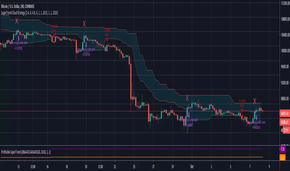
SuperTrend Cloud StrategyExperimental strategy to improve accuracy of SuperTrend Cloud. I am attempting to use STD deviation to manipulate the multiplier of the SuperTrend cloud. Greater STD Deviation = Oscillation in price action which can be applied to multiplier of SuperTrend to filter out bad trades and improve accuracy.
Noro's Triple RSI Top/Bottom v1.1In 1.1 added:
+ Leverage-parameter
+ Indicators-parameter
Strategy
It is the indicator. Threefold RSI . 3 different RSI indicators are used:
1) The RSI indicator with the period 2
2) The RSI indicator with the period 7
3) The RSI indicator with the period 14
If at the same time RSI-2 < 10 and RSI-7 < 20 and RSI-14 < 30 = a bottom
If at the same time RSI-2 > 90 and RSI-7 > 80 and RSI-14 > 70 = a top
Parameter accuracy influences.
Strategy allows to measure indicator accuracy. To check whether this indicator is suitable for this pair and a timeframe, how exact.

Noro's Triple RSI Top/BottomIt is the indicator. Threefold RSI. 3 different RSI indicators are used:
1) The RSI indicator with the period 2
2) The RSI indicator with the period 7
3) The RSI indicator with the period 14
If at the same time RSI-2 < 10 and RSI-7 < 20 and RSI-14 < 30 = a bottom
If at the same time RSI-2 > 90 and RSI-7 > 80 and RSI-14 > 70 = a top
Parameter accuracy influences.
Strategy allows to measure indicator accuracy. To check whether this indicator is suitable for this pair and a timeframe, how exact.

Volume Predictor [PhenLabs]📊 Volume Predictor
Version: PineScript™ v6
📌 Description
The Volume Predictor is an advanced technical indicator that leverages machine learning and statistical modeling techniques to forecast future trading volume. This innovative tool analyzes historical volume patterns to predict volume levels for upcoming bars, providing traders with valuable insights into potential market activity. By combining multiple prediction algorithms with pattern recognition techniques, the indicator delivers forward-looking volume projections that can enhance trading strategies and market analysis.
🚀 Points of Innovation:
Machine learning pattern recognition using Lorentzian distance metrics
Multi-algorithm prediction framework with algorithm selection
Ensemble learning approach combining multiple prediction methods
Real-time accuracy metrics with visual performance dashboard
Dynamic volume normalization for consistent scale representation
Forward-looking visualization with configurable prediction horizon
🔧 Core Components
Pattern Recognition Engine : Identifies similar historical volume patterns using Lorentzian distance metrics
Multi-Algorithm Framework : Offers five distinct prediction methods with configurable parameters
Volume Normalization : Converts raw volume to percentage scale for consistent analysis
Accuracy Tracking : Continuously evaluates prediction performance against actual outcomes
Advanced Visualization : Displays actual vs. predicted volume with configurable future bar projections
Interactive Dashboard : Shows real-time performance metrics and prediction accuracy
🔥 Key Features
The indicator provides comprehensive volume analysis through:
Multiple Prediction Methods : Choose from Lorentzian, KNN Pattern, Ensemble, EMA, or Linear Regression algorithms
Pattern Matching : Identifies similar historical volume patterns to project future volume
Adaptive Predictions : Generates volume forecasts for multiple bars into the future
Performance Tracking : Calculates and displays real-time prediction accuracy metrics
Normalized Scale : Presents volume as a percentage of historical maximums for consistent analysis
Customizable Visualization : Configure how predictions and actual volumes are displayed
Interactive Dashboard : View algorithm performance metrics in a customizable information panel
🎨 Visualization
Actual Volume Columns : Color-coded green/red bars showing current normalized volume
Prediction Columns : Semi-transparent blue columns representing predicted volume levels
Future Bar Projections : Forward-looking volume predictions with configurable transparency
Prediction Dots : Optional white dots highlighting future prediction points
Reference Lines : Visual guides showing the normalized volume scale
Performance Dashboard : Customizable panel displaying prediction method and accuracy metrics
📖 Usage Guidelines
History Lookback Period
Default: 20
Range: 5-100
This setting determines how many historical bars are analyzed for pattern matching. A longer period provides more historical data for pattern recognition but may reduce responsiveness to recent changes. A shorter period emphasizes recent market behavior but might miss longer-term patterns.
🧠 Prediction Method
Algorithm
Default: Lorentzian
Options: Lorentzian, KNN Pattern, Ensemble, EMA, Linear Regression
Selects the algorithm used for volume prediction:
Lorentzian: Uses Lorentzian distance metrics for pattern recognition, offering excellent noise resistance
KNN Pattern: Traditional K-Nearest Neighbors approach for historical pattern matching
Ensemble: Combines multiple methods with weighted averaging for robust predictions
EMA: Simple exponential moving average projection for trend-following predictions
Linear Regression: Projects future values based on linear trend analysis
Pattern Length
Default: 5
Range: 3-10
Defines the number of bars in each pattern for machine learning methods. Shorter patterns increase sensitivity to recent changes, while longer patterns may identify more complex structures but require more historical data.
Neighbors Count
Default: 3
Range: 1-5
Sets the K value (number of nearest neighbors) used in KNN and Lorentzian methods. Higher values produce smoother predictions by averaging more historical patterns, while lower values may capture more specific patterns but could be more susceptible to noise.
Prediction Horizon
Default: 5
Range: 1-10
Determines how many future bars to predict. Longer horizons provide more forward-looking information but typically decrease accuracy as the prediction window extends.
📊 Display Settings
Display Mode
Default: Overlay
Options: Overlay, Prediction Only
Controls how volume information is displayed:
Overlay: Shows both actual volume and predictions on the same chart
Prediction Only: Displays only the predictions without actual volume
Show Prediction Dots
Default: false
When enabled, adds white dots to future predictions for improved visibility and clarity.
Future Bar Transparency (%)
Default: 70
Range: 0-90
Controls the transparency of future prediction bars. Higher values make future bars more transparent, while lower values make them more visible.
📱 Dashboard Settings
Show Dashboard
Default: true
Toggles display of the prediction accuracy dashboard. When enabled, shows real-time accuracy metrics.
Dashboard Location
Default: Bottom Right
Options: Top Left, Top Right, Bottom Left, Bottom Right
Determines where the dashboard appears on the chart.
Dashboard Text Size
Default: Normal
Options: Small, Normal, Large
Controls the size of text in the dashboard for various display sizes.
Dashboard Style
Default: Solid
Options: Solid, Transparent
Sets the visual style of the dashboard background.
Understanding Accuracy Metrics
The dashboard provides key performance metrics to evaluate prediction quality:
Average Error
Shows the average difference between predicted and actual values
Positive values indicate the prediction tends to be higher than actual volume
Negative values indicate the prediction tends to be lower than actual volume
Values closer to zero indicate better prediction accuracy
Accuracy Percentage
A measure of how close predictions are to actual outcomes
Higher percentages (>70%) indicate excellent prediction quality
Moderate percentages (50-70%) indicate acceptable predictions
Lower percentages (<50%) suggest weaker prediction reliability
The accuracy metrics are color-coded for quick assessment:
Green: Strong prediction performance
Orange: Moderate prediction performance
Red: Weaker prediction performance
✅ Best Use Cases
Anticipate upcoming volume spikes or drops
Identify potential volume divergences from price action
Plan entries and exits around expected volume changes
Filter trading signals based on predicted volume support
Optimize position sizing by forecasting market participation
Prepare for potential volatility changes signaled by volume predictions
Enhance technical pattern analysis with volume projection context
⚠️ Limitations
Volume predictions become less accurate over longer time horizons
Performance varies based on market conditions and asset characteristics
Works best on liquid assets with consistent volume patterns
Requires sufficient historical data for pattern recognition
Sudden market events can disrupt prediction accuracy
Volume spikes may be muted in predictions due to normalization
💡 What Makes This Unique
Machine Learning Approach : Applies Lorentzian distance metrics for robust pattern matching
Algorithm Selection : Offers multiple prediction methods to suit different market conditions
Real-time Accuracy Tracking : Provides continuous feedback on prediction performance
Forward Projection : Visualizes multiple future bars with configurable display options
Normalized Scale : Presents volume as a percentage of maximum volume for consistent analysis
Interactive Dashboard : Displays key metrics with customizable appearance and placement
🔬 How It Works
The Volume Predictor processes market data through five main steps:
1. Volume Normalization:
Converts raw volume to percentage of maximum volume in lookback period
Creates consistent scale representation across different timeframes and assets
Stores historical normalized volumes for pattern analysis
2. Pattern Detection:
Identifies similar volume patterns in historical data
Uses Lorentzian distance metrics for robust similarity measurement
Determines strength of pattern match for prediction weighting
3. Algorithm Processing:
Applies selected prediction algorithm to historical patterns
For KNN/Lorentzian: Finds K nearest neighbors and calculates weighted prediction
For Ensemble: Combines multiple methods with optimized weighting
For EMA/Linear Regression: Projects trends based on statistical models
4. Accuracy Calculation:
Compares previous predictions to actual outcomes
Calculates average error and prediction accuracy
Updates performance metrics in real-time
5. Visualization:
Displays normalized actual volume with color-coding
Shows current and future volume predictions
Presents performance metrics through interactive dashboard
💡 Note:
The Volume Predictor performs optimally on liquid assets with established volume patterns. It’s most effective when used in conjunction with price action analysis and other technical indicators. The multi-algorithm approach allows adaptation to different market conditions by switching prediction methods. Pay special attention to the accuracy metrics when evaluating prediction reliability, as sudden market changes can temporarily reduce prediction quality. The normalized percentage scale makes the indicator consistent across different assets and timeframes, providing a standardized approach to volume analysis.

Intelligent Top & Bottom Finder v9.8 Keyvankh📈 Intelligent Top & Bottom Finder v9.8 Keyvankh
A next-generation all-in-one trading system for precise tops, bottoms, and reversals across all timeframes.
---
🟢 Overview
This indicator is a powerful and intelligent solution for detecting market tops and bottoms, key reversals, and S/R zones with institutional-grade accuracy. Designed for traders seeking an edge in any market (crypto, forex, stocks), it combines advanced candlestick recognition, multi-indicator confirmation, smart support/resistance clustering, and strict signal filtering into one seamless tool.
---
🔎 How Does It Work?
1. Advanced Support & Resistance Clustering
Automatically detects and draws high-probability support and resistance zones using dynamic ATR-based pivot clustering.
Highlights breakouts and retest (flip) zones in real-time, adapting to changing market structure.
2. Full Candlestick Pattern Recognition
Scans for 15+ classic and advanced patterns: Engulfing, Pin Bar, Doji, Three Bar, Marubozu, Hammer, Shooting Star, Three White Soldiers, Three Black Crows, Tweezer, Morning/Evening Star, Kicker, Belt Hold, and more.
Scores each pattern’s strength based on location (S/R zone, retest, breakout), volume context, and confirmation signals.
3. Multi-Indicator Confirmation Engine**
Integrates and scores confirmation from up to five additional sources:
RSI Games 1.2** (smoothed LTF momentum shifts)
MACD Divergence** (bullish/bearish momentum reversal)
QQE+ v7 Advanced** (dynamic volatility filter)
OBV Trend Filter** (volume-backed trend validation)
Volume Game** (net volume spike and reversal detection)
Each module can be enabled or disabled to fit your personal trading style.
4. Institutional S/R and Retest Logic
Real-time recognition of major trendline breaks, retest zones, and price flips.
Automatic labeling and coloring of S/R zones, retest boxes, and confirmation candles.
5. Smart Buy & Sell Signal Generation**
Combines all scoring modules with strict logical filters and “failsafe override” logic (guaranteeing signal on confirmed hammers, engulfings, etc. even if other filters disagree).
Plots clear “BUY” and “SELL” labels only when a strong, multi-factor signal appears—minimizing noise and maximizing reliability.
Built-in fallback logic (optional) for edge cases.
6. Alerts & Automation Ready
TradingView alerts for all BUY, SELL, or ANY signal conditions—perfect for auto-trading or notification setups.
---
*⚙️ Customizable Inputs
Enable/Disable any module (RSI Games, MACD, OBV, QQE+, Candlestick Scanner, Volume Game)
Minimum Confirmations** required for a signal (1–10)
Pivot/Zone Sensitivity:** ATR multiplier, pivots per cluster, retest bar duration
LTF (Lower Timeframe) Confirmation:** Fully configurable
---
📊 How To Use**
Apply on any timeframe and symbol**—crypto, stocks, forex, indices.
Use as a **standalone reversal/entry tool** or to confirm your own technical setups.
Combine with your favorite momentum, trend, or volume indicators for advanced confluence.
Set up **TradingView alerts** for auto-trading, Telegram/email notifications, or trade journaling.
---
🟢 What Makes This Unique?
All-in-one multi-indicator fusion:** No more juggling a dozen scripts.
Institutional logic:** Goes beyond basic signals with true S/R, retest, and volume logic.
Full transparency:** Source code is clear and commented (if published open-source).
Fast and reliable:** Optimized for minimal lag and maximum accuracy.
---
⚠️ Disclaimer**
This indicator is a tool to assist with trade timing and risk management. **No system is 100% accurate.** Always use in conjunction with your own analysis and risk management practices.
---
📚 Credits & License**
Created by Keyvan Khodakhah.
You may use, modify, or share this script under the (mozilla.org).
Please credit the original author if you fork or reuse in public.
---
Questions, feedback, or collaboration? Contact: Keyvankh
---
Precision in technical analysis comes from layers of confluence and discipline. This tool brings that precision to your chart.
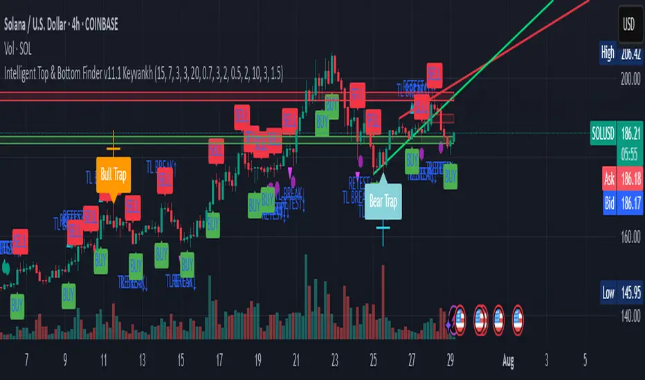
Deadzone Pro @DaviddTechDeadzone Pro by @DaviddTech – Adaptive Multi-Strategy NNFX Trading System
Deadzone Pro by @DaviddTech is a meticulously engineered trading indicator that strictly adheres to the No-Nonsense Forex (NNFX) methodology. It integrates adaptive trend detection, dual confirmation indicators, advanced volatility filtering, and dynamic risk management into one powerful, visually intuitive system. Ideal for traders seeking precision and clarity, this indicator consistently delivers high-probability trade setups across all market conditions.
🔥 Key Features:
The Setup:
Adaptive Hull Moving Average Baseline: Clearly identifies trend direction using an advanced, gradient-colored Hull MA that intensifies based on trend strength, providing immediate visual clarity.
Dual Confirmation Indicators: Combines Waddah Attar Explosion (momentum detector) and Bull/Bear Power (strength gauge) for robust validation, significantly reducing false entries.
Volatility Filter (ADX): Ensures entries are only made during strong trending markets, filtering out weak, range-bound scenarios for enhanced trade accuracy.
Dynamic Trailing Stop Loss: Implements a SuperTrend-based trailing stop using adaptive ATR calculations, managing risk effectively while optimizing exits.
Dashboard:
💎 Gradient Visualization & User Interface:
Dynamic gradient colors enhance readability, clearly indicating bullish/bearish strength.
Comprehensive dashboard summarizes component statuses, real-time market sentiment, and entry conditions at a glance.
Distinct and clear buy/sell entry and exit signals, with adaptive stop-loss levels visually plotted.
Candlestick coloring based on momentum signals (Waddah Attar) for intuitive market reading.
📈 How to Interpret Signals:
Bullish Signal: Enter when Hull MA baseline trends upward, both confirmation indicators align bullish, ADX indicates strong trend (>25), and price breaks above the previous trailing stop.
Bearish Signal: Enter short or exit long when Hull MA baseline trends downward, confirmations indicate bearish momentum, ADX confirms trend strength, and price breaks below previous trailing stop.
📊 Recommended Usage:
Timeframes: Ideal on 1H, 4H, and Daily charts for swing trading; effective on shorter (5M, 15M) charts for day trading.
Markets: Compatible with Forex, Crypto, Indices, Stocks, and Commodities.
The Entry & Exit:
🎯 Trading Styles:
Choose from three distinct trading modes:
Conservative: Requires full alignment of all indicators for maximum accuracy.
Balanced (Default): Optimized balance between signal frequency and reliability.
Aggressive: Fewer confirmations needed for more frequent trading signals.
📝 Credits & Originality:
Deadzone Pro incorporates advanced concepts inspired by:
Hull Moving Average by @Julien_Eche
Waddah Attar Explosion by @LazyBear
Bull Bear Power by @Pinecoders
ADX methodology by @BeikabuOyaji
This system has been significantly refactored and enhanced by @DaviddTech to maximize synergy, clarity, and usability, standing apart distinctly from its original components.
Deadzone Pro exemplifies precision and discipline, aligning fully with NNFX principles to provide traders with a comprehensive yet intuitive trading advantage.
ML Deep Regression Pro (TechnoBlooms)ML Deep Regression Pro is a machine-learning-inspired trading indicator that integrates Polynomial Regression, Linear Regression and Statistical Deviation models to provide a powerful, data-driven approach to market trend analysis.
Designed for traders, quantitative analysts and developers, this tool transforms raw market data into predictive trend insights, allowing for better decision-making and trend validation.
By leveraging statistical regression techniques, ML Deep Regression Pro eliminates market noise and identifies key trend shifts, making it a valuable addition to both manual and algorithmic trading strategies.
REGRESSION ANALYSIS
Regression is a statistical modeling technique used in machine learning and data science to identify patterns and relationships between variables. In trading, it helps detect price trends, reversals and volatility changes by fitting price data into a predictive model.
1. Linear Regression -
The most widely used regression model in trading, providing a best-fit plotted line to track price trends.
2. Polynomial Regression -
A more advanced form of regression that fits curved price structures, capturing complex market cycles and improving trend forecasting accuracy.
3. Standard Deviation Bands -
Based on regression calculations, these bands measure price dispersion and identify overbought/ oversold conditions, similar to Bollinger Bands. By default, these lines are hidden and user can make it visible through Settings.
KEY FEATURES :-
✅ Hybrid Regression Engine – Combines Linear and Polynomial Regression to detect market trends with greater accuracy.
✅ Dynamic Trend Bias Analysis – Identifies bullish & bearish market conditions using real-time regression models.
✅ Standard Deviation Bands – Measures price volatility and potential reversals with an advanced deviation model.
✅ Adaptive EMA Crossover Signals – Generates buy/sell signals when price momentum shifts relative to the regression trend.

Quantum Motion Oscillator-QMO (TechnoBlooms)Quantum Motion Oscillator (QMO) is a momentum indicator designed for traders who demand precision. Combining multi-timeframe weighted linear regression with EMA crossovers, QMO offers a dynamic view of market momentum, helping traders anticipate trend shifts with greater accuracy.
This oscillator is inspired by quantum mechanics and wave theory, where market movement is seen as a series of probabilistic waves rather than rigid structures.
The histogram is plotted in proportion to the price movement of the candlesticks.
KEY FEATURES
1. Multi-Timeframe Histogram - Integrates 1 to 5 weighted linear regression averages, reducing lag while maintaining accuracy.
2. EMA Crossover Signal - Uses a Short and Long EMA to confirm trend shifts with minimal noise.
3. Adaptive Trend Analysis - Self-adjusting mechanics make QMO effective in both ranging and trending markets.
4. Scalable for Different Trading Styles - Works seamlessly for scalping, intraday, swing and position trading.
ADVANCED PROFESSIONAL INSIGHTS
1. Wave Dynamics and Market Flow - Inspired by wave mechanics, QMO reflects the energy accumulation and dissipation in price movements.
Expanding histogram waves = Strong momentum surge
Contracting waves = Momentum weakening, potential reversal zone.
2. Liquidity and Order Flow Applications - QMO works well alongside liquidity concepts and smart money techniques:
Combine with Fair Value Gaps & Order Blocks -> Enter when QMO signals align with liquidity zones.
Avoid False Moves - If price sweeps liquidity, but QMO momentum diverges, it is a sign of potential smart money manipulation.
Shavarie's MCV IndicatorShavarie's MCV Indicator (MACD + CCI + Volume Delta) is a custom-built trend-following and volume-based indicator that helps traders confirm market direction with high accuracy. It combines the MACD (Moving Average Convergence Divergence), CCI (Commodity Channel Index), and Volume Delta, ensuring that all three indicators align before making a trading decision. The goal is to filter out false signals and provide high-probability trade setups.
History & Development
Shavarie's MCV Indicator was developed by Shavarie Gordon, an experienced swing trader, to improve trend confirmation on Gold (XAUUSD) and other markets. After testing various indicators, Shavarie discovered that MACD, CCI, and Volume Delta together provide the best combination of trend strength, momentum, and real-time volume flow. This indicator was designed to eliminate lagging signals, improve win rates, and enhance market timing for both swing and scalping strategies.
How It Works & Calculations
MACD (Moving Average Convergence Divergence)
Measures momentum and trend strength using the difference between a 12-period EMA and a 26-period EMA.
The MACD line and Signal line crossover confirms buy/sell signals.
A rising MACD histogram confirms bullish strength, while a falling histogram confirms bearish strength.
CCI (Commodity Channel Index)
Measures how far the price is from its statistical average.
Above +100 → Overbought (strong trend continuation or reversal).
Below -100 → Oversold (strong trend continuation or reversal).
When CCI aligns with MACD, it confirms momentum strength.
Volume Delta
Measures the difference between buying and selling volume in real time.
A positive delta means more aggressive buying (bullish).
A negative delta means more aggressive selling (bearish).
Helps confirm MACD and CCI trends by showing real volume strength.
Key Takeaways & Features
✅ No false signals: All three indicators must align before entering a trade.
✅ Trend confirmation: Ensures momentum and volume agree before trading.
✅ Works on multiple timeframes: Designed for swing trading on the daily and scalping on 45 min + 5 min.
✅ Great for Gold & Metals: Optimized for XAUUSD, XAUJPY, XAU/AUD, and possibly Palladium (XPDUSD).
✅ Custom-built by a professional trader: Developed by Shavarie Gordon after extensive testing.
Summary
Shavarie’s MCV Indicator is a powerful and reliable trading tool that combines momentum, trend, and volume analysis. By ensuring that MACD, CCI, and Volume Delta align, it eliminates false signals and increases trade accuracy. Whether used for swing trading or scalping, this indicator helps traders enter high-probability trades with confidence.
DataDoodles SD + ProbabilityDataDoodles SD + Probability
Overview:
The “DataDoodles SD + Probability” indicator is designed to provide traders with a statistical edge by leveraging standard deviation and probability metrics. This advanced tool calculates the annualized standard deviation, Z-score, and probability of price movements, offering insights into potential market direction with customizable alert thresholds.
Key Features:
1. Annualized Standard Deviation (Volatility) Calculation:
• Uses a user-defined period to compute the rolling standard deviation of daily returns.
• Annualizes the volatility, giving a clear picture of expected price fluctuations.
2. Probability of Price Movement:
• Calculates the probability of price moving up or down using a corrected Z-Score.
• Displays the probability percentage for both upward and downward movements.
3. Dynamic Alerts:
• Configurable alerts for upward and downward price movement probabilities.
• Receive alerts when the probability exceeds user-defined thresholds.
4. Projections and Visuals:
• Plots projected high and low price levels based on annualized volatility.
• Displays Z-Score and probability metrics on the chart for quick reference.
5. Comprehensive Data Table:
• Bottom-center table displays key metrics:
• Daily Return
• Standard Deviation (SD)
• Annualized Standard Deviation (Yearly SD)
User Inputs:
• Annualization Period: Set the time frame for volatility annualization (Default: 252 days).
• SD Period: Define the rolling window for calculating standard deviation (Default: 252 days).
• Alert Probability Up/Down: Customize the probability thresholds for alerts (Default: 90%).
How It Works:
• Data Request and Calculation:
• Uses daily close prices to ensure consistent timeframe calculations.
• Calculates daily returns and annualizes the volatility using the square root of the time frame.
• Probability Computation:
• Employs a normal distribution CDF approximation to compute the probability of upward and downward price movements.
• Adjusts probabilities based on Z-Score to ensure accuracy.
• High and Low Projections:
• Utilizes the annualized volatility to estimate high and low price projections for the year.
• Visual Indicators and Alerts:
• Plots projected high (green) and low (red) levels on the chart.
• Displays Z-Score, probability percentages, and dynamically updates a statistics table.
Use Cases:
• Trend Analysis: Identify high-probability market movements using the probability metrics.
• Volatility Insights: Understand annualized volatility to gauge market risk and potential price ranges.
• Strategic Trading Decisions: Set alerts for high-probability scenarios to optimize entry and exit points.
Why Use “DataDoodles SD + Probability”?
This indicator provides a powerful combination of statistical analysis and visual representation. It empowers traders with:
• Quantitative Edge: By leveraging probability metrics and standard deviation, users can make informed trading decisions.
• Risk Management: Annualized volatility projections help in setting realistic stop-loss and take-profit levels.
• Actionable Alerts: Customizable probability alerts ensure users are notified of potential market moves, allowing proactive trading strategies.
Recommended Settings:
• Annualization Period: 252 (Ideal for daily data representing a trading year)
• SD Period: 252 (One trading year for consistent volatility calculations)
• Alert Probability: Set to 90% for conservative signals or lower for more frequent alerts.
Final Thoughts:
The “DataDoodles SD + Probability” indicator is a robust tool for traders looking to integrate statistical analysis into their trading strategies. It combines volatility measurement, probability calculations, and dynamic alerts to provide a comprehensive market overview.
Whether you’re a day trader or a long-term investor, this indicator can enhance your market insight and improve decision-making accuracy.
Disclaimer:
This indicator is a technical analysis tool designed for educational purposes. Past performance is not indicative of future results. Traders are encouraged to perform their own analysis and manage risk accordingly.