DataDoodles SD + ProbabilityDataDoodles SD + Probability
Overview:
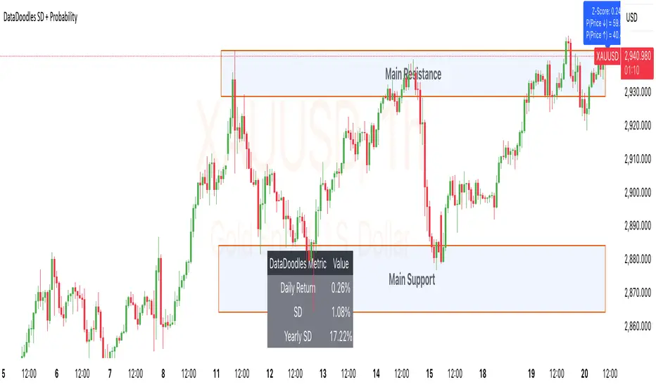
The “DataDoodles SD + Probability” indicator is designed to provide traders with a statistical edge by leveraging standard deviation and probability metrics. This advanced tool calculates the annualized standard deviation, Z-score, and probability of price movements, offering insights into potential market direction with customizable alert thresholds.
Key Features:
1. Annualized Standard Deviation (Volatility) Calculation:
• Uses a user-defined period to compute the rolling standard deviation of daily returns.
• Annualizes the volatility, giving a clear picture of expected price fluctuations.
2. Probability of Price Movement:
• Calculates the probability of price moving up or down using a corrected Z-Score.
• Displays the probability percentage for both upward and downward movements.
3. Dynamic Alerts:
• Configurable alerts for upward and downward price movement probabilities.
• Receive alerts when the probability exceeds user-defined thresholds.
4. Projections and Visuals:
• Plots projected high and low price levels based on annualized volatility.
• Displays Z-Score and probability metrics on the chart for quick reference.
5. Comprehensive Data Table:
• Bottom-center table displays key metrics:
• Daily Return
• Standard Deviation (SD)
• Annualized Standard Deviation (Yearly SD)
User Inputs:
• Annualization Period: Set the time frame for volatility annualization (Default: 252 days).
• SD Period: Define the rolling window for calculating standard deviation (Default: 252 days).
• Alert Probability Up/Down: Customize the probability thresholds for alerts (Default: 90%).
How It Works:
• Data Request and Calculation:
• Uses daily close prices to ensure consistent timeframe calculations.
• Calculates daily returns and annualizes the volatility using the square root of the time frame.
• Probability Computation:
• Employs a normal distribution CDF approximation to compute the probability of upward and downward price movements.
• Adjusts probabilities based on Z-Score to ensure accuracy.
• High and Low Projections:
• Utilizes the annualized volatility to estimate high and low price projections for the year.
• Visual Indicators and Alerts:
• Plots projected high (green) and low (red) levels on the chart.
• Displays Z-Score, probability percentages, and dynamically updates a statistics table.
Use Cases:
• Trend Analysis: Identify high-probability market movements using the probability metrics.
• Volatility Insights: Understand annualized volatility to gauge market risk and potential price ranges.
• Strategic Trading Decisions: Set alerts for high-probability scenarios to optimize entry and exit points.
Why Use “DataDoodles SD + Probability”?
This indicator provides a powerful combination of statistical analysis and visual representation. It empowers traders with:
• Quantitative Edge: By leveraging probability metrics and standard deviation, users can make informed trading decisions.
• Risk Management: Annualized volatility projections help in setting realistic stop-loss and take-profit levels.
• Actionable Alerts: Customizable probability alerts ensure users are notified of potential market moves, allowing proactive trading strategies.
Recommended Settings:
• Annualization Period: 252 (Ideal for daily data representing a trading year)
• SD Period: 252 (One trading year for consistent volatility calculations)
• Alert Probability: Set to 90% for conservative signals or lower for more frequent alerts.
Final Thoughts:
The “DataDoodles SD + Probability” indicator is a robust tool for traders looking to integrate statistical analysis into their trading strategies. It combines volatility measurement, probability calculations, and dynamic alerts to provide a comprehensive market overview.
Whether you’re a day trader or a long-term investor, this indicator can enhance your market insight and improve decision-making accuracy.
Disclaimer:
This indicator is a technical analysis tool designed for educational purposes. Past performance is not indicative of future results. Traders are encouraged to perform their own analysis and manage risk accordingly.
Cerca negli script per "accuracy"
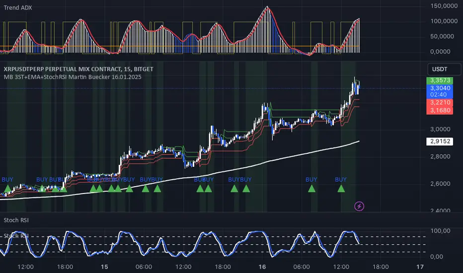
MB 3ST+EMA+StochRSI Martin Buecker 16.01.2025Short Description of the Indicator "MB 3ST+EMA+StochRSI Martin Buecker 16.01.2025"
This trend-following and momentum-based indicator combines Supertrend, EMA 200, and Stochastic RSI to generate buy and sell signals with improved accuracy.
1. Key Components
Supertrend (3 variations):
Uses three Supertrend indicators with different periods to confirm trend direction.
Buy signal when at least 2 Supertrends are bearish.
Sell signal when at least 2 Supertrends are bullish.
EMA 200 (Exponential Moving Average):
Buy signals only when the price is above EMA 200 (uptrend confirmation).
Sell signals only when the price is below EMA 200 (downtrend confirmation).
Multi-Timeframe Stochastic RSI:
Uses a higher timeframe Stoch RSI (default: 15 minutes) to filter signals.
Buy signal when %K crosses above %D (bullish momentum).
Sell signal when %K crosses below %D (bearish momentum).
2. Signal Generation
📈 Buy Signal Conditions:
✅ At least 2 of 3 Supertrends are bearish
✅ Price is above EMA 200
✅ Stoch RSI shows a bullish crossover (%K > %D)
📉 Sell Signal Conditions:
✅ At least 2 of 3 Supertrends are bullish
✅ Price is below EMA 200
✅ Stoch RSI shows a bearish crossover (%K < %D)
3. Visual Representation & Alerts
Supertrend Lines:
Green = Bullish, Red = Bearish
EMA 200: White Line
Buy/Sell Signals:
Green triangle (below bar) = Buy
Red triangle (above bar) = Sell
Alerts:
Notifies users when a buy or sell signal is triggered.
Background Coloring:
Green for Buy signals, Red for Sell signals
4. Purpose & Benefits
🔥 Combines trend (EMA 200, Supertrend) and momentum analysis (Stoch RSI) for better signal accuracy.
🔥 Works best in trending markets, filtering out false signals in sideways movements.
🔥 Suitable for scalping and day trading, providing clear and structured trade entries.
Turtle Soup ICT Strategy [TradingFinder] FVG + CHoCH/CSD🔵 Introduction
The ICT Turtle Soup trading setup, designed in the ICT style, operates by hunting or sweeping liquidity zones to exploit false breakouts and failed breakouts in key liquidity Zones, such as recent highs, lows, or major support and resistance levels.
This setup identifies moments when the price breaches these liquidity zones, triggering stop orders placed (Stop Hunt) by other traders, and then quickly reverses direction. These movements are often associated with liquidity sweeps that create temporary market imbalances.
The reversal is typically confirmed by one of three structural shifts : a Market Structure Shift (MSS), a Change of Character (CHoCH), or a break of the Change in State of Delivery (CISD). Each of these structural shifts provides a reliable signal to interpret market intent and align trading decisions with the expected price movement. After the structural shift, the price frequently pullback to a Fair Value Gap (FVG), offering a precise entry point for trades.
By integrating key concepts such as liquidity, liquidity sweeps, stop order activation, structural shifts (MSS, CHoCH, CISD), and price imbalances, the ICT Turtle Soup setup enables traders to identify reversal points and key entry zones with high accuracy.
This strategy is highly versatile, making it applicable across markets such as forex, stocks, cryptocurrencies, and futures. It offers traders a robust and systematic approach to understanding price movements and optimizing their trading strategies
🟣 Bullish and Bearish Setups
Bullish Setup : The price first sweeps below a Sell-Side Liquidity (SSL) zone, then reverses upward after forming an MSS or CHoCH, and finally pulls back to an FVG, creating a buying opportunity.
Bearish Setup : The price first sweeps above a Buy-Side Liquidity (BSL) zone, then reverses downward after forming an MSS or CHoCH, and finally pulls back to an FVG, creating a selling opportunity.
🔵 How to Use
To effectively utilize the ICT Turtle Soup trading setup, begin by identifying key liquidity zones, such as recent highs, lows, or support and resistance levels, in higher timeframes.
Then, monitor lower timeframes for a Liquidity Sweep and confirmation of a Market Structure Shift (MSS) or Change of Character (CHoCH).
After the structural shift, the price typically pulls back to an FVG, offering an optimal trade entry point. Below, the bullish and bearish setups are explained in detail.
🟣 Bullish Turtle Soup Setup
Identify Sell-Side Liquidity (SSL) : In a higher timeframe (e.g., 1-hour or 4-hour), identify recent price lows or support levels that serve as SSL zones, typically the location of stop-loss orders for traders.
Observe a Liquidity Sweep : On a lower timeframe (e.g., 15-minute or 30-minute), the price must move below one of these liquidity zones and then reverse. This movement indicates a liquidity sweep.
Confirm Market Structure Shift : After the price reversal, look for a structural shift (MSS or CHoCH) indicated by the formation of a Higher Low (HL) and Higher High (HH).
Enter the Trade : Once the structural shift is confirmed, the price typically pulls back to an FVG. Enter a buy trade in this zone, set a stop-loss slightly below the recent low, and target Buy-Side Liquidity (BSL) in the higher timeframe for profit.
🟣 Bearish Turtle Soup Setup
Identify Buy-Side Liquidity (BSL) : In a higher timeframe, identify recent price highs or resistance levels that serve as BSL zones, typically the location of stop-loss orders for traders.
Observe a Liquidity Sweep : On a lower timeframe, the price must move above one of these liquidity zones and then reverse. This movement indicates a liquidity sweep.
Confirm Market Structure Shift : After the price reversal, look for a structural shift (MSS or CHoCH) indicated by the formation of a Lower High (LH) and Lower Low (LL).
Enter the Trade : Once the structural shift is confirmed, the price typically pulls back to an FVG. Enter a sell trade in this zone, set a stop-loss slightly above the recent high, and target Sell-Side Liquidity (SSL) in the higher timeframe for profit.
🔵 Settings
Higher TimeFrame Levels : This setting allows you to specify the higher timeframe (e.g., 1-hour, 4-hour, or daily) for identifying key liquidity zones.
Swing period : You can set the swing detection period.
Max Swing Back Method : It is in two modes "All" and "Custom". If it is in "All" mode, it will check all swings, and if it is in "Custom" mode, it will check the swings to the extent you determine.
Max Swing Back : You can set the number of swings that will go back for checking.
FVG Length : Default is 120 Bar.
MSS Length : Default is 80 Bar.
FVG Filter : This refines the number of identified FVG areas based on a specified algorithm to focus on higher quality signals and reduce noise.
Types of FVG filter s:
Very Aggressive Filter: Adds a condition where, for an upward FVG, the last candle's highest price must exceed the middle candle's highest price, and for a downward FVG, the last candle's lowest price must be lower than the middle candle's lowest price. This minimally filters out FVGs.
Aggressive Filter: Builds on the Very Aggressive mode by ensuring the middle candle is not too small, filtering out more FVGs.
Defensive Filter: Adds criteria regarding the size and structure of the middle candle, requiring it to have a substantial body and specific polarity conditions, filtering out a significant number of FVGs.
Very Defensive Filter: Further refines filtering by ensuring the first and third candles are not small-bodied doji candles, retaining only the highest quality signals.
In the indicator settings, you can customize the visibility of various elements, including MSS, FVG, and HTF Levels. Additionally, the color of each element can be adjusted to match your preferences. This feature allows traders to tailor the chart display to their specific needs, enhancing focus on the key data relevant to their strategy.
🔵 Conclusion
The ICT Turtle Soup trading setup is a powerful tool in the ICT style, enabling traders to exploit false breakouts in key liquidity zones. By combining concepts of liquidity, liquidity sweeps, market structure shifts (MSS and CHoCH), and pullbacks to FVG, this setup helps traders identify precise reversal points and execute trades with reduced risk and increased accuracy.
With applications across various markets, including forex, stocks, crypto, and futures, and its customizable indicator settings, the ICT Turtle Soup setup is ideal for both beginner and advanced traders. By accurately identifying liquidity zones in higher timeframes and confirming structure shifts in lower timeframes, this setup provides a reliable strategy for navigating volatile market conditions.
Ultimately, success with this setup requires consistent practice, precise market analysis, and proper risk management, empowering traders to make smarter decisions and achieve their trading goals.

Bitcoin Macro Trend Map [Ox_kali]
## Introduction
__________________________________________________________________________________
The “Bitcoin Macro Trend Map” script is designed to provide a comprehensive analysis of Bitcoin’s macroeconomic trends. By leveraging a unique combination of Bitcoin-specific macroeconomic indicators, this script helps traders identify potential market peaks and troughs with greater accuracy. It synthesizes data from multiple sources to offer a probabilistic view of market excesses, whether overbought or oversold conditions.
This script offers significant value for the following reasons:
1. Holistic Market Analysis : It integrates a diverse set of indicators that cover various aspects of the Bitcoin market, from investor sentiment and market liquidity to mining profitability and network health. This multi-faceted approach provides a more complete picture of the market than relying on a single indicator.
2. Customization and Flexibility : Users can customize the script to suit their specific trading strategies and preferences. The script offers configurable parameters for each indicator, allowing traders to adjust settings based on their analysis needs.
3. Visual Clarity : The script plots all indicators on a single chart with clear visual cues. This includes color-coded indicators and background changes based on market conditions, making it easy for traders to quickly interpret complex data.
4. Proven Indicators : The script utilizes well-established indicators like the EMA, NUPL, PUELL Multiple, and Hash Ribbons, which are widely recognized in the trading community for their effectiveness in predicting market movements.
5. A New Comprehensive Indicator : By integrating background color changes based on the aggregate signals of various indicators, this script essentially creates a new, comprehensive indicator tailored specifically for Bitcoin. This visual representation provides an immediate overview of market conditions, enhancing the ability to spot potential market reversals.
Optimal for use on timeframes ranging from 1 day to 1 week , the “Bitcoin Macro Trend Map” provides traders with actionable insights, enhancing their ability to make informed decisions in the highly volatile Bitcoin market. By combining these indicators, the script delivers a robust tool for identifying market extremes and potential reversal points.
## Key Indicators
__________________________________________________________________________________
Macroeconomic Data: The script combines several relevant macroeconomic indicators for Bitcoin, such as the 10-month EMA, M2 money supply, CVDD, Pi Cycle, NUPL, PUELL, MRVR Z-Scores, and Hash Ribbons (Full description bellow).
Open Source Sources: Most of the scripts used are sourced from open-source projects that I have modified to meet the specific needs of this script.
Recommended Timeframes: For optimal performance, it is recommended to use this script on timeframes ranging from 1 day to 1 week.
Objective: The primary goal is to provide a probabilistic solution to identify market excesses, whether overbought or oversold points.
## Originality and Purpose
__________________________________________________________________________________
This script stands out by integrating multiple macroeconomic indicators into a single comprehensive tool. Each indicator is carefully selected and customized to provide insights into different aspects of the Bitcoin market. By combining these indicators, the script offers a holistic view of market conditions, helping traders identify potential tops and bottoms with greater accuracy. This is the first version of the script, and additional macroeconomic indicators will be added in the future based on user feedback and other inputs.
## How It Works
__________________________________________________________________________________
The script works by plotting each macroeconomic indicator on a single chart, allowing users to visualize and interpret the data easily. Here’s a detailed look at how each indicator contributes to the analysis:
EMA 10 Monthly: Uses an exponential moving average over 10 monthly periods to signal bullish and bearish trends. This indicator helps identify long-term trends in the Bitcoin market by smoothing out price fluctuations to reveal the underlying trend direction.Moving Averages w/ 18 day/week/month.
Credit to @ryanman0
M2 Money Supply: Analyzes the evolution of global money supply, indicating market liquidity conditions. This indicator tracks the changes in the total amount of money available in the economy, which can impact Bitcoin’s value as a hedge against inflation or economic instability.
Credit to @dylanleclair
CVDD (Cumulative Value Days Destroyed): An indicator based on the cumulative value of days destroyed, useful for identifying market turning points. This metric helps assess the Bitcoin market’s health by evaluating the age and value of coins that are moved, indicating potential shifts in market sentiment.
Credit to @Da_Prof
Pi Cycle: Uses simple and exponential moving averages to detect potential sell points. This indicator aims to identify cyclical peaks in Bitcoin’s price, providing signals for potential market tops.
Credit to @NoCreditsLeft
NUPL (Net Unrealized Profit/Loss): Measures investors’ unrealized profit or loss to signal extreme market levels. This indicator shows the net profit or loss of Bitcoin holders as a percentage of the market cap, helping to identify periods of significant market optimism or pessimism.
Credit to @Da_Prof
PUELL Multiple: Assesses mining profitability relative to historical averages to indicate buying or selling opportunities. This indicator compares the daily issuance value of Bitcoin to its yearly average, providing insights into when the market is overbought or oversold based on miner behavior.
Credit to @Da_Prof
MRVR Z-Scores: Compares market value to realized value to identify overbought or oversold conditions. This metric helps gauge the overall market sentiment by comparing Bitcoin’s market value to its realized value, identifying potential reversal points.
Credit to @Pinnacle_Investor
Hash Ribbons: Uses hash rate variations to signal buying opportunities based on miner capitulation and recovery. This indicator tracks the health of the Bitcoin network by analyzing hash rate trends, helping to identify periods of miner capitulation and subsequent recoveries as potential buying opportunities.
Credit to @ROBO_Trading
## Indicator Visualization and Interpretation
__________________________________________________________________________________
For each horizontal line representing an indicator, a legend is displayed on the right side of the chart. If the conditions are positive for an indicator, it will turn green, indicating the end of a bearish trend. Conversely, if the conditions are negative, the indicator will turn red, signaling the end of a bullish trend.
The background color of the chart changes based on the average of green or red indicators. This parameter is configurable, allowing adjustment of the threshold at which the background color changes, providing a clear visual indication of overall market conditions.
## Script Parameters
__________________________________________________________________________________
The script includes several configurable parameters to customize the display and behavior of the indicators:
Color Style:
Normal: Default colors.
Modern: Modern color style.
Monochrome: Monochrome style.
User: User-customized colors.
Custom color settings for up trends (Up Trend Color), down trends (Down Trend Color), and NaN (NaN Color)
Background Color Thresholds:
Thresholds: Settings to define the thresholds for background color change.
Low/High Red Threshold: Low and high thresholds for bearish trends.
Low/High Green Threshold: Low and high thresholds for bullish trends.
Indicator Display:
Options to show or hide specific indicators such as EMA 10 Monthly, CVDD, Pi Cycle, M2 Money, NUPL, PUELL, MRVR Z-Scores, and Hash Ribbons.
Specific Indicator Settings:
EMA 10 Monthly: Options to customize the period for the exponential moving average calculation.
M2 Money: Aggregation of global money supply data.
CVDD: Adjustments for value normalization.
Pi Cycle: Settings for simple and exponential moving averages.
NUPL: Thresholds for unrealized profit/loss values.
PUELL: Adjustments for mining profitability multiples.
MRVR Z-Scores: Settings for overbought/oversold values.
Hash Ribbons: Options for hash rate moving averages and capitulation/recovery signals.
## Conclusion
__________________________________________________________________________________
The “Bitcoin Macro Trend Map” by Ox_kali is a tool designed to analyze the Bitcoin market. By combining several macroeconomic indicators, this script helps identify market peaks and troughs. It is recommended to use it on timeframes from 1 day to 1 week for optimal trend analysis. The scripts used are sourced from open-source projects, modified to suit the specific needs of this analysis.
## Notes
__________________________________________________________________________________
This is the first version of the script and it is still in development. More indicators will likely be added in the future. Feedback and comments are welcome to improve this tool.
## Disclaimer:
__________________________________________________________________________________
Please note that the Open Interest liquidation map is not a guarantee of future market performance and should be used in conjunction with proper risk management. Always ensure that you have a thorough understanding of the indicator’s methodology and its limitations before making any investment decisions. Additionally, past performance is not indicative of future results.

PhiSmoother Moving Average Ribbon [ChartPrime]DSP FILTRATION PRIMER:
DSP (Digital Signal Processing) filtration plays a critical role with financial indication analysis, involving the application of digital filters to extract actionable insights from data. Its primary trading purpose is to distinguish and isolate relevant signals separate from market noise, allowing traders to enhance focus on underlying trends and patterns. By smoothing out price data, DSP filters aid with trend detection, facilitating the formulation of more effective trading techniques.
Additionally, DSP filtration can play an impactful role with detecting support and resistance levels within financial movements. By filtering out noise and emphasizing significant price movements, identifying key levels for entry and exit points become more apparent. Furthermore, DSP methods are instrumental in measuring market volatility, enabling traders to assess volatility levels with improved accuracy.
In summary, DSP filtration techniques are versatile tools for traders and analysts, enhancing decision-making processes in financial markets. By mitigating noise and highlighting relevant signals, DSP filtration improves the overall quality of trading analysis, ultimately leading to better conclusions for market participants.
APPLYING FIR FILTERS:
FIR (Finite Impulse Response) filters are indispensable tools in the realm of financial analysis, particularly for trend identification and characterization within market data. These filters effectively smooth out price fluctuations and noise, enabling traders to discern underlying trends with greater fidelity. By applying FIR filters to price data, robust trading strategies can be developed with grounded trend-following principles, enhancing their ability to capitalize on market movements.
Moreover, FIR filter applications extend into wide-ranging utility within various fields, one being vital for informed decision-making in analysis. These filters help identify critical price levels where assets may tend to stall or reverse direction, providing traders with valuable insights to aid with identification of optimal entry and exit points within their indicator arsenal. FIRs are undoubtedly a cornerstone to modern trading innovation.
Additionally, FIR filters aid in volatility measurement and analysis, allowing traders to gauge market volatility accurately and adjust their risk management approaches accordingly. By incorporating FIR filters into their analytical arsenal, traders can improve the quality of their decision-making processes and achieve better trading outcomes when contending with highly dynamic market conditions.
INTRODUCTORY DEBUT:
ChartPrime's " PhiSmoother Moving Average Ribbon " indicator aims to mark a significant advancement in technical analysis methodology by removing unwanted fluctuations and disturbances while minimizing phase disturbance and lag. This indicator introduces PhiSmoother, a powerful FIR filter in it's own right comparable to Ehlers' SuperSmoother.
PhiSmoother leverages a custom tailored FIR filter to smooth out price fluctuations by mitigating aliasing noise problematic to identification of underlying trends with accuracy. With adjustable parameters such as phase control, traders can fine-tune the indicator to suit their specific analytical needs, providing a flexible and customizable solution.
Mathemagically, PhiSmoother incorporates various color coding preferences, enabling traders to visualize trends more effectively on a volatile landscape. Whether utilizing progression, chameleon, or binary color schemes, you can more fluidly interpret market dynamics and make informed visual decisions regarding entry and exit points based on color-coded plotting.
The indicator's alert system further enhances its utility by providing notifications of specifically chosen filter crossings. Traders can customize alert modes and messages while ensuring they stay informed about potential opportunities aligned with their trading style.
Overall, the "PhiSmoother Moving Average Ribbon" visually stands out as a revolutionary mechanism for technical analysis, offering traders a comprehensive solution for trend identification, visualization, and alerting within financial markets to achieve advantageous outcomes.
NOTEWORTHY SETTINGS FEATURES:
Price Source Selection - The indicator offers flexibility in choosing the price source for analysis. Traders can select from multiple options.
Phase Control Parameter - One of the notable standout features of this indicator is the phase control parameter. Traders can fine-tune the phase or lag of the indicator to adapt it to different market conditions or timeframes. This feature enables optimization of the indicator's responsiveness to price movements and align it with their specific trading tactics.
Coloring Preferences - Another magical setting is the coloring features, one being "Chameleon Color Magic". Traders can customize the color scheme of the indicator based on their visual preferences or to improve interpretation. The indicator offers options such as progression, chameleon, or binary color schemes, all having versatility to dynamically visualize market trends and patterns. Two colors may be specifically chosen to reduce overlay indicator interference while also contrasting for your visual acuity.
Alert Controls - The indicator provides diverse alert controls to manage alerts for specific market events, depending on their trading preferences.
Alertable Crossings: Receive an alert based on selectable predefined crossovers between moving average neighbors
Customizable Alert Messages: Traders can personalize alert messages with preferred information details
Alert Frequency Control: The frequency of alerts is adjustable for maximum control of timely notifications

Price Depth Analysis to the MAHello Traders! Today, I bring you an indicator that can greatly assist you in your trading. This indicator aims to analyze the Expansion and Contraction process of the price in relation to a moving average. We refer to "Expansion" when the price moves away from the moving average; a significant expansion could signal that the asset is in a strong trend. On the other hand, when we refer to "Contraction", it's when the price approaches or returns to the moving average. A contraction could signal that the asset is losing momentum and might be preparing for a trend change or consolidation.
To use the indicator, the first thing you need to do is define the type of analysis you want to perform (from the indicator settings) whether you want to evaluate prices above the moving average or below. You should also select the type of moving average and its period.
The indicator will search for the maximum distance in all the chart bars, which will be represented with a yellow label.
From that value, the indicator will generate a certain number of proportional levels (configurable up to 20) and will count all the bars that reached each level. This will be represented in a table showing both the number of bars that reached each range and the percentage in relation to the total bars of all ranges.
Additionally, there's the possibility to view the ranges directly for the current price, providing a good reference.
>> Alerts:
The indicator comes with alerts that notify traders about specific price movements in relation to a moving average (MA). These alerts are triggered when the price enters different ranges, either above or below the MA.
>> Settings:
- Type of Analysis: Users can choose to analyze the price either above or below the MA.
- Length of the moving average: Length of the MA.
- Source of the moving average: Source to calculate the MA (e.g., close, open).
- Type of moving average: Type of MA (SMA, EMA, WMA, VWMA, HMA).
- Show Moving Average: Option to display or hide the MA on the chart.
- Number of levels: Number of levels or ranges to categorize the distance between the price and the MA.
- Number of decimals: Number of decimals to display in labels and tables.
- Show Ranges: Option to display or hide the ranges on the chart.
- Extend Range: Extension of the ranges into future bars.
- Range Fill Transparency: Transparency of the range fill.
>> Potential Utility of the Indicator:
- Entry and Exit Optimization:
By understanding the percentages of each range, traders can identify optimal levels to enter or exit a trade, maximizing profits and minimizing losses.
- Risk Management:
Range percentages can help determine market volatility. A range with a high percentage indicates greater volatility, which can be useful for setting wider stop losses or adjusting position size.
- Overbought and Oversold Zone Identification:
If a price is at the upper or lower extreme of its percentage range, it may indicate overbought or oversold conditions, respectively. These zones can be opportunities for counter-trend trades.
- Momentum Assessment:
A rapid change in range percentages can indicate strong momentum in a particular direction. Traders can use this information to ride the momentum wave or prepare for a potential reversal.
- False Signal Filtering:
By combining range percentage knowledge with other indicators, traders can filter out signals that might be less reliable, thus improving trade accuracy.
- Strategic Planning:
Knowing range percentages allows traders to adapt their strategies according to market conditions. For instance, in a market with narrow ranges and low percentages, they might opt for range strategies. In markets with wide ranges and high percentages, they might look for trend strategies.
- Trend Strength Evaluation:
If range percentages show that the price consistently stays at one end of the range, this may signal a strong and sustained trend.
- Improved Trading Discipline:
By basing trading decisions on quantitative data like range percentages, traders can trade more objectively and disciplined, avoiding impulsive or emotion-based decisions.
>> Future Indicator Update:
- In future versions, we plan to incorporate a detailed analysis based on the historical behavior of candles after the price enters a specific range. For instance, if after an upward movement the price enters a certain range and historically, the next candle tends to be bearish in a high percentage of occasions, this information will be highlighted and presented clearly to the user. The idea behind this addition is to provide traders with a statistical edge, allowing them to anticipate potential market movements with greater accuracy. Moreover, this information could be used to seek trading opportunities in smaller timeframes, aligning the trade direction based on the probability of this mentioned candle.
>> Conclusions:
- In summary, a detailed understanding of each range's percentages in an indicator provides traders with a valuable tool to analyze the market, make informed decisions, and enhance their trading. By grasping the significance of these percentages, traders can adapt their strategies and techniques to fully leverage the opportunities the market presents.

Crypto Terminal [Kioseff Trading]Hello!
Introducing Crypto Terminal (:
The indicator makes use of cryptocurrency data provided by vendor INTOTHEBLOCK.
NOTE: The cryptocurrency on your chart must be paired with USD or USDT. Data won't load otherwise - possibly transient. For instance, BTCUSD or BTCUSDT, ETHUSD or ETHUSDT.
Provided datasets:
Twitter Sentiment Data
Telegram Sentiment Data
Whale Data (i.e. % of Asset Belonging to Whales)
$100,000+ Transactions
Bulls/Bears (Bulls Buying | Bears Selling)
Current Position PnL (Currently Open Positions for the Coin are Retrieved and Plotted. Data is Split into Currently Profitable Positions, Losing Positions, and B/E Positions)
Average Balance
Holders/Traders Percentage (Addresses are Retrieved and Classified as Holding Accounts or Trader Accounts)
Correlation
Futures OI
Perpetual OI
Zero Balance Addresses
Flow (Money Inflow & Outflow)
Active Addresses
Average Transaction Time
Realized PnL (Addresses with Realized Profits, Realized Losses, and B/E)
Cruisers
A few more data points are provided.
Additionally, you can plot the values of any dataset in a pane below price.
Below are images of plottable data; different cryptocurrencies will be shown for each example (:
Twitter sentiment data.
Assess this data lightly; difficult to confirm accuracy.
Telegram sentiment data.
Assess this data lightly; difficult to confirm accuracy.
Percentage of asset belonging to whales.
$100,000+ transactions (volume oriented)
Bulls buying; bears selling.
Current positions at profit; current positions at loss; current positions at breakeven.
Average balance.
Percentage of asset belonging to traders; percentage of asset belonging to holders.
Asset's 30-interval correlation to BTC.
Perpetual open interest.
Zero-balance addresses.
Flows.
Active addresses.
Average transaction time.
Addresses at realized profit; addresses at realized loss; addresses at breakeven.
Cruiser data.
Futures open interest.
Naturally, this data isn't provided for every cryptocurrency; NaN values are returned in some instances.
Table 1
I provided three data tables, which load independently, so you don't have to change plotted data to access values.
Table 2
Lastly, you can create a 10-asset crypto index and run calculations against it.
The image shows an example.
I'll update this script with additional calculations/data in the near future. If you've any suggestions - please let me know!
Enjoy (:

Noro's SILA v1.2Noro's SILA v1.2 - these are 5 trend indicators in 1, for the sake of better accuracy.
Added:
1) Settings
2) Arrows
Noro's SILA v1.2 uses 5 trend indicators:
1) SuperTrend
2) DI Plus-Minus
3) WOW trend indicator (my idea)
4) BarColor indicator (my idea)
5) BestMA (or "BMA") indicator (my idea)
The user can switch-off any indicator from 5 to achieve big accuracy.
How does it work?
Each indicator from 5 defines a trend in own way. If two indicators report that there will be a uptrend, and three others the indicator report that there will be a downtrend - it is downtrend (a red background).
For an example
Now SuperTrend = uptrend = +1
Now DI Plus-Minus = downtrend = -1
Now WOW trend indicator = downtrend = -1
Now BarColor indicator = downtrend = -1
Now BestMA (or "BMA") indicator = uptrend = +1
Sum = + 1 - 1 - 1 - 1 + 1 = -1 = downtrend
If sum > 0 = uptrend
Sensivity
The user himself chooses what there will be a sensitivity (in settings).
If sensivity = 3:
sum > or = 3 - uptrend
sum < or = -3 - downtrend
sum > -3 and < 3 - NA-color of background
Trendlines
3 lower trendlines (blue plots) is "sum+3"
5 upper trendlines is "sum-5"
etc
Settings:
1) sensivity - you see above
2) distance - distance between the price and lines (for convenience)

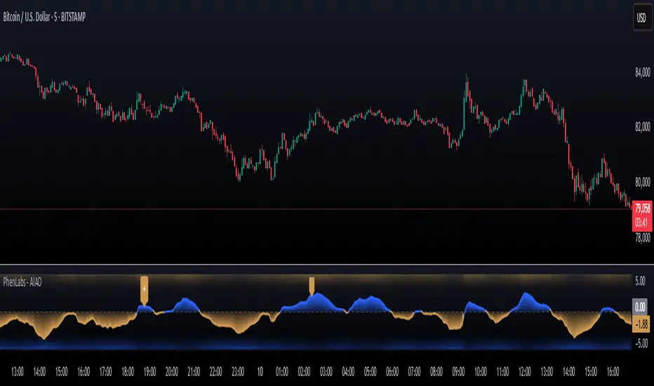
AI Adaptive Oscillator [PhenLabs]📊 Algorithmic Adaptive Oscillator
Version: PineScript™ v6
📌 Description
The AI Adaptive Oscillator is a sophisticated technical indicator that employs ensemble learning and adaptive weighting techniques to analyze market conditions. This innovative oscillator combines multiple traditional technical indicators through an AI-driven approach that continuously evaluates and adjusts component weights based on historical performance. By integrating statistical modeling with machine learning principles, the indicator adapts to changing market dynamics, providing traders with a responsive and reliable tool for market analysis.
🚀 Points of Innovation:
Ensemble learning framework with adaptive component weighting
Performance-based scoring system using directional accuracy
Dynamic volatility-adjusted smoothing mechanism
Intelligent signal filtering with cooldown and magnitude requirements
Signal confidence levels based on multi-factor analysis
🔧 Core Components
Ensemble Framework : Combines up to five technical indicators with performance-weighted integration
Adaptive Weighting : Continuous performance evaluation with automated weight adjustment
Volatility-Based Smoothing : Adapts sensitivity based on current market volatility
Pattern Recognition : Identifies potential reversal patterns with signal qualification criteria
Dynamic Visualization : Professional color schemes with gradient intensity representation
Signal Confidence : Three-tiered confidence assessment for trading signals
🔥 Key Features
The indicator provides comprehensive market analysis through:
Multi-Component Ensemble : Integrates RSI, CCI, Stochastic, MACD, and Volume-weighted momentum
Performance Scoring : Evaluates each component based on directional prediction accuracy
Adaptive Smoothing : Automatically adjusts based on market volatility
Pattern Detection : Identifies potential reversal patterns in overbought/oversold conditions
Signal Filtering : Prevents excessive signals through cooldown periods and minimum change requirements
Confidence Assessment : Displays signal strength through intuitive confidence indicators (average, above average, excellent)
🎨 Visualization
Gradient-Filled Oscillator : Color intensity reflects strength of market movement
Clear Signal Markers : Distinct bullish and bearish pattern signals with confidence indicators
Range Visualization : Clean representation of oscillator values from -6 to 6
Zero Line : Clear demarcation between bullish and bearish territory
Customizable Colors : Color schemes that can be adjusted to match your chart style
Confidence Symbols : Intuitive display of signal confidence (no symbol, +, or ++) alongside direction markers
📖 Usage Guidelines
⚙️ Settings Guide
Color Settings
Bullish Color
Default: #2b62fa (Blue)
This setting controls the color representation for bullish movements in the oscillator. The color appears when the oscillator value is positive (above zero), with intensity indicating the strength of the bullish momentum. A brighter shade indicates stronger bullish pressure.
Bearish Color
Default: #ce9851 (Amber)
This setting determines the color representation for bearish movements in the oscillator. The color appears when the oscillator value is negative (below zero), with intensity reflecting the strength of the bearish momentum. A more saturated shade indicates stronger bearish pressure.
Signal Settings
Signal Cooldown (bars)
Default: 10
Range: 1-50
This parameter sets the minimum number of bars that must pass before a new signal of the same type can be generated. Higher values reduce signal frequency and help prevent overtrading during choppy market conditions. Lower values increase signal sensitivity but may generate more false positives.
Min Change For New Signal
Default: 1.5
Range: 0.5-3.0
This setting defines the minimum required change in oscillator value between consecutive signals of the same type. It ensures that new signals represent meaningful changes in market conditions rather than minor fluctuations. Higher values produce fewer but potentially higher-quality signals, while lower values increase signal frequency.
AI Core Settings
Base Length
Default: 14
Minimum: 2
This fundamental setting determines the primary calculation period for all technical components in the ensemble (RSI, CCI, Stochastic, etc.). It represents the lookback window for each component’s base calculation. Shorter periods create a more responsive but potentially noisier oscillator, while longer periods produce smoother signals with potential lag.
Adaptive Speed
Default: 0.1
Range: 0.01-0.3
Controls how quickly the oscillator adapts to new market conditions through its volatility-adjusted smoothing mechanism. Higher values make the oscillator more responsive to recent price action but potentially more erratic. Lower values create smoother transitions but may lag during rapid market changes. This parameter directly influences the indicator’s adaptiveness to market volatility.
Learning Lookback Period
Default: 150
Minimum: 10
Determines the historical data range used to evaluate each ensemble component’s performance and calculate adaptive weights. This setting controls how far back the AI “learns” from past performance to optimize current signals. Longer periods provide more stable weight distribution but may be slower to adapt to regime changes. Shorter periods adapt more quickly but may overreact to recent anomalies.
Ensemble Size
Default: 5
Range: 2-5
Specifies how many technical components to include in the ensemble calculation.
Understanding The Interaction Between Settings
Base Length and Learning Lookback : The base length determines the reactivity of individual components, while the lookback period determines how their weights are adjusted. These should be balanced according to your timeframe - shorter timeframes benefit from shorter base lengths, while the lookback should generally be 10-15 times the base length for optimal learning.
Adaptive Speed and Signal Cooldown : These settings control sensitivity from different angles. Increasing adaptive speed makes the oscillator more responsive, while reducing signal cooldown increases signal frequency. For conservative trading, keep adaptive speed low and cooldown high; for aggressive trading, do the opposite.
Ensemble Size and Min Change : Larger ensembles provide more stable signals, allowing for a lower minimum change threshold. Smaller ensembles might benefit from a higher threshold to filter out noise.
Understanding Signal Confidence Levels
The indicator provides three distinct confidence levels for both bullish and bearish signals:
Average Confidence (▲ or ▼) : Basic signal that meets the minimum pattern and filtering criteria. These signals indicate potential reversals but with moderate confidence in the prediction. Consider using these as initial alerts that may require additional confirmation.
Above Average Confidence (▲+ or ▼+) : Higher reliability signal with stronger underlying metrics. These signals demonstrate greater consensus among the ensemble components and/or stronger historical performance. They offer increased probability of successful reversals and can be traded with less additional confirmation.
Excellent Confidence (▲++ or ▼++) : Highest quality signals with exceptional underlying metrics. These signals show strong agreement across oscillator components, excellent historical performance, and optimal signal strength. These represent the indicator’s highest conviction trade opportunities and can be prioritized in your trading decisions.
Confidence assessment is calculated through a multi-factor analysis including:
Historical performance of ensemble components
Degree of agreement between different oscillator components
Relative strength of the signal compared to historical thresholds
✅ Best Use Cases:
Identify potential market reversals through oscillator extremes
Filter trade signals based on AI-evaluated component weights
Monitor changing market conditions through oscillator direction and intensity
Confirm trade signals from other indicators with adaptive ensemble validation
Detect early momentum shifts through pattern recognition
Prioritize trading opportunities based on signal confidence levels
Adjust position sizing according to signal confidence (larger for ++ signals, smaller for standard signals)
⚠️ Limitations
Requires sufficient historical data for accurate performance scoring
Ensemble weights may lag during dramatic market condition changes
Higher ensemble sizes require more computational resources
Performance evaluation quality depends on the learning lookback period length
Even high confidence signals should be considered within broader market context
💡 What Makes This Unique
Adaptive Intelligence : Continuously adjusts component weights based on actual performance
Ensemble Methodology : Combines strength of multiple indicators while minimizing individual weaknesses
Volatility-Adjusted Smoothing : Provides appropriate sensitivity across different market conditions
Performance-Based Learning : Utilizes historical accuracy to improve future predictions
Intelligent Signal Filtering : Reduces noise and false signals through sophisticated filtering criteria
Multi-Level Confidence Assessment : Delivers nuanced signal quality information for optimized trading decisions
🔬 How It Works
The indicator processes market data through five main components:
Ensemble Component Calculation :
Normalizes traditional indicators to consistent scale
Includes RSI, CCI, Stochastic, MACD, and volume components
Adapts based on the selected ensemble size
Performance Evaluation :
Analyzes directional accuracy of each component
Calculates continuous performance scores
Determines adaptive component weights
Oscillator Integration :
Combines weighted components into unified oscillator
Applies volatility-based adaptive smoothing
Scales final values to -6 to 6 range
Signal Generation :
Detects potential reversal patterns
Applies cooldown and magnitude filters
Generates clear visual markers for qualified signals
Confidence Assessment :
Evaluates component agreement, historical accuracy, and signal strength
Classifies signals into three confidence tiers (average, above average, excellent)
Displays intuitive confidence indicators (no symbol, +, ++) alongside direction markers
💡 Note:
The AI Adaptive Oscillator performs optimally when used with appropriate timeframe selection and complementary indicators. Its adaptive nature makes it particularly valuable during changing market conditions, where traditional fixed-weight indicators often lose effectiveness. The ensemble approach provides a more robust analysis by leveraging the collective intelligence of multiple technical methodologies. Pay special attention to the signal confidence indicators to optimize your trading decisions - excellent (++) signals often represent the most reliable trade opportunities.
[blackcat] L2 FiboKAMA Adaptive TrendOVERVIEW
The L2 FiboKAMA Adaptive Trend indicator leverages advanced technical analysis techniques by integrating Fibonacci principles with the Kaufman Adaptive Moving Average (KAMA). This combination creates a dynamic and responsive tool designed to adapt seamlessly to changing market conditions. By providing clear buy and sell signals based on adaptive momentum, this indicator helps traders identify potential entry and exit points effectively. Its intuitive design and robust features make it a valuable addition to any trader’s arsenal 📊💹.
According to the principle of Kaufman's Adaptive Moving Average (KAMA), it is a type of moving average line specifically designed for markets with high volatility. Unlike traditional moving averages, KAMA can automatically adjust its period based on market conditions to improve accuracy and responsiveness. This makes it particularly useful for capturing market trends and reducing false signals in varying market environments.
The use of Fibonacci magic numbers (3, 8, 13) enhances the performance and accuracy of KAMA. These numbers have special mathematical properties that align well with the changing trends of KAMA moving averages. Combining them with KAMA can significantly boost its effectiveness, making it a popular choice among traders seeking reliable signals.
This fusion not only smoothens price fluctuations but also ensures quick responses to market changes, offering dependable entry and exit points. Thanks to the flexibility and precision of KAMA combined with Fibonacci magic numbers, traders can better manage risks and aim for higher returns.
FEATURES
Enhanced Kaufman Adaptive Moving Average (KAMA): Incorporates Fibonacci principles for improved adaptability:
Source Price: Allows customization of the price series used for calculation (default: HLCC4).
Fast Length: Determines the period for quicker adjustments to recent price changes.
Slow Length: Sets the period for smoother transitions over longer-term trends.
Dynamic Lines:
KAMA Line: A yellow line representing the primary adaptive moving average, which adapts quickly to new trends.
Trigger Line: A fuchsia line serving as a reference point for detecting crossovers and generating signals.
Visual Cues:
Buy Signals: Green 'B' labels indicating potential buying opportunities.
Sell Signals: Red 'S' labels signaling possible selling points.
Fill Areas: Colored regions between the KAMA and Trigger lines to visually represent trend directions and strength.
Alert Functionality: Generates real-time alerts for both buy and sell signals, ensuring timely notifications for actionable insights 🔔.
Customizable Parameters: Offers flexibility through adjustable inputs, allowing users to tailor the indicator to their specific trading strategies and preferences.
HOW TO USE
Adding the Indicator:
Open your TradingView chart and navigate to the indicators list.
Select L2 FiboKAMA Adaptive Trend and add it to your chart.
Configuring Parameters:
Adjust the Source Price to choose the desired price series (e.g., close, open, high, low).
Set the Fast Length to define how quickly the indicator responds to recent price movements.
Configure the Slow Length to determine the smoothness of long-term trend adaptations.
Interpreting Signals:
Monitor the chart for green 'B' labels indicating buy signals and red 'S' labels for sell signals.
Observe the colored fill areas between the KAMA and Trigger lines to gauge trend strength and direction.
Setting Up Alerts:
Enable alerts within the indicator settings to receive notifications whenever buy or sell signals are triggered.
Customize alert messages and frequencies according to your trading plan.
Combining with Other Tools:
Integrate this indicator with additional technical analysis tools and fundamental research for comprehensive decision-making.
Confirm signals using other indicators like RSI, MACD, or Bollinger Bands for increased reliability.
Optimizing Performance:
Backtest the indicator across various assets and timeframes to understand its behavior under different market conditions.
Fine-tune parameters based on historical performance and current market dynamics.
Integrating Magic Numbers:
Understand the basic principles of KAMA to find suitable entry points for Fibonacci magic numbers.
Utilize the efficiency ratio to measure market volatility and adjust moving average parameters accordingly.
Apply Fibonacci magic numbers (3, 8, 13) to enhance the responsiveness and accuracy of KAMA.
LIMITATIONS
Market Volatility: May produce false signals during periods of extreme volatility or sideways movement.
Parameter Sensitivity: Requires careful tuning of fast and slow lengths to balance responsiveness and stability.
Asset-Specific Behavior: Effectiveness can vary significantly across different financial instruments and time horizons.
Complementary Analysis: Should be used alongside other analytical methods to enhance accuracy and reduce risk.
NOTES
Historical Data: Ensure adequate historical data availability for precise calculations and backtesting.
Demo Testing: Thoroughly test the indicator on demo accounts before deploying it in live trading environments.
Continuous Learning: Stay updated with market trends and continuously refine your strategy incorporating feedback from the indicator's performance.
Risk Management: Always implement proper risk management practices regardless of the signals provided by the indicator.
ADVANCED USAGE TIPS
Multi-Timeframe Analysis: Apply the indicator across multiple timeframes to gain deeper insights into underlying trends.
Divergence Strategy: Look for divergences between price action and the KAMA line to spot potential reversals early.
Volume Integration: Combine volume analysis with the indicator to confirm the strength of identified trends.
Custom Scripting: Modify the script to include additional filters or conditions tailored to your unique trading approach.
IMPROVING KAMA PERFORMANCE
Increase Length: Extend the KAMA length to consider more historical data, reducing the impact of short-term price fluctuations.
Adjust Fast and Slow Lengths: Make KAMA smoother by increasing the fast length and decreasing the slow length.
Use Smoothing Factor: Apply a smoothing factor to control the level of smoothness; typical values range from 0 to 1.
Combine with Other Indicators: Pair KAMA with other smoothing indicators like EMA or SMA for more reliable signals.
Filter Noise: Use filters or other technical analysis tools to eliminate price noise, enhancing KAMA's effectiveness.
Money Flow Index Crossover IndicatorThe "Money Flow Index Crossover Indicator" is a specialized technical analysis tool designed to assist traders by providing a clear visualization of potential buy and sell signals based on the Money Flow Index (MFI) and its smoothed moving average (SMA). This indicator delineates overbought and oversold zones, offering valuable insights into market dynamics. It operates as an oscillator on a separate pane, helping traders identify bullish and bearish market conditions with greater precision. By incorporating k-Nearest Neighbor (KNN) machine learning techniques, this indicator enhances the reliability and accuracy of the signals provided.
Originality and Usefulness:
This script is not just a simple mashup of existing indicators but integrates multiple components to create a unique and comprehensive analysis tool. The combined information from the MFI, its smoothed moving average, and the KNN machine learning techniques influence the form and accuracy of the Money Flow Index Average line and the Smoothed Money Flow Index line giving a visually helpful representation of overbought and oversold conditions. These lines are displayed in an oscillator style crossover, allowing users to visualize potential buy and sell zones for setting up potential signals. The user can adjust various settings of these tools behind the code to fine-tune the behavior and sensitivity of these lines. This integration provides a more robust and insightful trading tool that can adapt to different market conditions and trading styles.
How It Works:
Inputs:
MFI Settings:
Show Signals: Allows users to toggle the display of MFI and SMA crossing signals, which are critical for identifying potential market reversals.
Plot Amount: Determines the number of plots in the heat map, ranging from 2 to 28, enabling customization based on user preference.
Source: Defines the data source for MFI calculations, typically set to OHLC4 for a balanced view of price movements.
Smooth Initial MFI Length: Specifies the smoothing length for the initial MFI calculations to reduce noise and enhance signal clarity.
MFI SMA Length: Sets the length for the SMA used to smooth the MFI average, providing a more stable reference line.
Machine Learning Settings:
Use KInSource: Option to average MFI data by adding a lookback to the source, improving the accuracy of historical comparisons.
KNN Distance Requirement: Defines the distance calculation method for KNN (Max, Min, Both) to refine the data filtering process.
Machine Learning Length: Specifies the amount of machine learning data stored for smoothing results, balancing between responsiveness and stability.
KNN Length: Sets the number of KNN used to calculate the allowable distance range, enhancing the precision of the machine learning model.
Fast and Slow Lengths: Defines the lengths for fast and slow MFI calculations, allowing the indicator to capture different market dynamics.
Smoothing Length: Determines the length at which MFI calculations start for a more smoothed result, reducing false signals.
Variables and Functions:
KNN Function: Filters machine learning data to calculate valid distances based on defined criteria, ensuring more accurate MFI averages.
MFI Calculations: Computes both fast and slow MFI values, applies smoothing, and stores them for KNN processing to refine signal generation.
MFI KNN Calculation: Uses the KNN function to calculate the machine learning average of MFI values, enhancing signal reliability.
MFI Average and SMA: Calculates the average and smoothed MFI values, which are crucial for determining crossover signals.
Calculations:
MFI Values: Calculates current fast and slow MFI values and applies smoothing to reduce market noise.
Storage Arrays: Stores MFI data in arrays for KNN processing, enabling historical comparison and pattern recognition.
KNN Processing: Computes the machine learning average of MFI values using the KNN function, improving the robustness of signals.
MFI Average: Scales the MFI average to fit the heat map and calculates the smoothed SMA, providing a clear visual representation of trends.
Crossover Signals: Identifies bullish (MFI crossing above SMA) and bearish (MFI crossing below SMA) signals, which are key for making trading decisions.
Plots and Visuals:
MFI Average and SMA Lines: Plots the MFI average and smoothed SMA on the chart, allowing traders to easily visualize market trends and potential reversals.
Zones: Defines and plots overbought, neutral, and oversold zones for easy visualization. The recommended settings for these zones are:
Overbought Zone: Level set to approximately 24.6, indicating a potential market top.
Neutral Zone: Level set to 14, representing a balanced market condition.
Oversold Zone: Level set to 5.4, signaling a potential market bottom.
Crossover Marks: Plots circles on the chart to indicate bullish and bearish crossover signals, making it easier to spot entry and exit points.
Visual Alerts:
Bullish and Bearish Alerts: one can see overbought and oversold conditions and up alert conditions for bullish and bearish MFI crossover signals, enabling traders to have access to visual cues when these events are on trajectory to occur and, if they occur, act promptly with the visual representation of its zones.
Why It's Helpful:
The "Money Flow Index Crossover Indicator" provides traders with a sophisticated tool to identify potential buy and sell conditions based on the combined information of the MFI and its smoothed moving average. The KNN machine learning techniques enhance the accuracy of this indicator's clear visual representation of overbought, neutral, and oversold zones. This combination of data represented on the chart helps traders make informed decisions about market conditions. This indicator is particularly useful for traders looking to refine their entry and exit points by leveraging advanced data analysis in respect to overbought and oversold conditions.
Disclaimer:
This indicator is intended to assist traders in making informed decisions based on technical analysis. However, it is not a guarantee of future performance and should be used in conjunction with other analysis techniques and risk management practices. Past performance is not indicative of future results, and traders should exercise caution and perform their own due diligence before making any trading decisions.

Intrabar Volume Delta — RealTime + History (Stocks/Crypto/Forex)Intrabar Volume Delta Grid — RealTime + History (Stocks/Crypto/Forex)
# Short Description
Shows intrabar Up/Down volume, Delta (absolute/relative) and UpShare% in a compact grid for both real-time and historical bars. Includes an MTF (M1…D1) dashboard, contextual coloring, density controls, and alerts on Δ and UpShare%. Smart historical splitting (“History Mode”) for Crypto/Futures/FX.
---
# What it does (Quick)
* **UpVol / DownVol / Δ / UpShare%** — visualizes order-flow inside each candle.
* **Real-time** — accumulates intrabar volume live by tick-direction.
* **History Mode** — splits Up/Down on closed bars via simple or range-aware logic.
* **MTF Dashboard** — one table view across M1, M5, M15, M30, H1, H4, D1 (Vol, Up/Down, Δ%, Share, Trend).
* **Contextual opacity** — stronger signals appear bolder.
* **Label density** — draw every N-th bar and limit to last X bars for performance.
* **Alerts** — thresholds for |Δ|, Δ%, and UpShare%.
---
# How it works (Real-Time vs History)
* **Real-time (open bar):** volume increments into **UpVolRT** or **DownVolRT** depending on last price move (↑ goes to Up, ↓ to Down). This approximates live order-flow even when full tick history isn’t available.
* **History (closed bars):**
* **None** — no split (Up/Down = 0/0). Safest for equities/indices with unreliable tick history.
* **Approx (Close vs Open)** — all volume goes to candle direction (green → Up 100%, red → Down 100%). Fast but yields many 0/100% bars.
* **Price Action Based** — splits by Close position within High-Low range; strength = |Close−mid|/(High−Low). Above mid → more Up; below mid → more Down. Falls back to direction if High==Low.
* **Auto** — **Stocks/Index → None**, **Crypto/Futures/FX → Approx**. If you see too many 0/100 bars, switch to **Price Action Based**.
---
# Rows & Meaning
* **Volume** — total bar volume (no split).
* **UpVol / DownVol** — directional intrabar volume.
* **Delta (Δ)** — UpVol − DownVol.
* **Absolute**: raw units
* **Relative (Δ%)**: Δ / (Up+Down) × 100
* **Both**: shows both formats
* **UpShare%** — UpVol / (Up+Down) × 100. >50% bullish, <50% bearish.
* Helpful icons: ▲ (>65%), ▼ (<35%).
---
# MTF Dashboard (🔧 Enable Dashboard)
A single table with **Vol, Up, Down, Δ%, Share, Trend (🔼/🔽/⏭️)** for selected timeframes (M1…D1). Great for a fast “panorama” read of flow alignment across horizons.
---
# Inputs (Grouped)
## Display
* Toggle rows: **Volume / Up / Down / Delta / UpShare**
* **Delta Display**: Absolute / Relative / Both
## Realtime & History
* **History Mode**: Auto / None / Approx / Price Action Based
* **Compact Numbers**: 1.2k, 1.25M, 3.4B…
## Theme & UI
* **Theme Mode**: Auto / Light / Dark
* **Row Spacing**: vertical spacing between rows
* **Top Row Y**: moves the whole grid vertically
* **Draw Guide Lines**: faint dotted guides
* **Text Size**: Tiny / Small / Normal / Large
## 🔧 Dashboard Settings
* **Enable Dashboard**
* **📏 Table Text Size**: Tiny…Huge
* **🦓 Zebra Rows**
* **🔲 Table Border**
## ⏰ Timeframes (for Dashboard)
* **M1…D1** toggles
## Contextual Coloring
* **Enable Contextual Coloring**: opacity by signal strength
* **Δ% cap / Share offset cap**: saturation caps
* **Min/Max transparency**: solid vs faint extremes
## Label Density & Size
* **Show every N-th bar**: draw labels only every Nth bar
* **Limit to last X bars**: keep labels only in the most recent X bars
## Colors
* Up / Down / Text / Guide
## Alerts
* **Delta Threshold (abs)** — |Δ| in volume units
* **UpShare > / <** — bullish/bearish thresholds
* **Enable Δ% Alert**, **Δ% > +**, **Δ% < −** — relative delta levels
---
# How to use (Quick Start)
1. Add the indicator to your chart (overlay=false → separate pane).
2. **History Mode**:
* Crypto/Futures/FX → keep **Auto** or switch to **Price Action Based** for richer history.
* Stocks/Index → prefer **None** or **Price Action Based** for safer splits.
3. **Label Density**: start with **Limit to last X bars = 30–150** and **Show every N-th bar = 2–4**.
4. **Contextual Coloring**: keep on to emphasize strong Δ% / Share moves.
5. **Dashboard**: enable and pick only the TFs you actually use.
6. **Alerts**: set thresholds (ideas below).
---
# Alerts (in TradingView)
Add alert → pick this indicator → choose any of:
* **Delta exceeds threshold** (|Δ| > X)
* **UpShare above threshold** (UpShare% > X)
* **UpShare below threshold** (UpShare% < X)
* **Relative Delta above +X%**
* **Relative Delta below −X%**
**Starter thresholds (tune per symbol & TF):**
* **Crypto M1/M5**: Δ% > +25…35 (bullish), Δ% < −25…−35 (bearish)
* **FX (tick volume)**: UpShare > 60–65% or < 40–35%
* **Stocks (liquid)**: set **Absolute Δ** by typical volume scale (e.g., 50k / 100k / 500k)
---
# Notes by Market Type
* **Crypto/Futures**: 24/7 and high liquidity — **Price Action Based** often gives nicer history splits than Approx.
* **Forex (FX)**: TradingView volume is typically **tick volume** (not true exchange volume). Treat Δ/Share as tick-based flow, still very useful intraday.
* **Stocks/Index**: historical tick detail can be limited. **None** or **Price Action Based** is a safer default. If you see too many 0/100% shares, switch away from Approx.
---
# “All Timeframes” accuracy
* Works on **any TF** (M1 → D1/W1).
* **Real-time accuracy** is strong for the open bar (live accumulation).
* **Historical accuracy** depends on your **History Mode** (None = safest, Approx = fastest/simplest, Price Action Based = more nuanced).
* The MTF dashboard uses `request.security` and therefore follows the same logic per TF.
---
# Trade Ideas (Use-Cases)
* **Scalping (M1–M5)**: a spike in Δ% + UpShare>65% + rising total Vol → momentum entries.
* **Intraday (M5–M30–H1)**: when multiple TFs show aligned Δ%/Share (e.g., M5 & M15 bullish), join the trend.
* **Swing (H4–D1)**: persistent Δ% > 0 and UpShare > 55–60% → structural accumulation bias.
---
# Advantages
* **True-feeling live flow** on the open bar.
* **Adaptable history** (three modes) to match data quality.
* **Clean visual layout** with guides, compact numbers, contextual opacity.
* **MTF snapshot** for quick bias read.
* **Performance controls** (last X bars, every N-th bar).
---
# Limitations & Care
* **FX uses tick volume** — interpret Δ/Share accordingly.
* **History Mode is an approximation** — confirm with trend/structure/liquidity context.
* **Illiquid symbols** can produce noisy or contradictory signals.
* **Too many labels** can slow charts → raise N, lower X, or disable guides.
---
# Best Practices (Checklist)
* Crypto/Futures: prefer **Price Action Based** for history.
* Stocks: **None** or **Price Action Based**; be cautious with **Approx**.
* FX: pair Δ% & UpShare% with session context (London/NY) and volatility.
* If labels overlap: tweak **Row Spacing** and **Text Size**.
* In the dashboard, keep only the TFs you actually act on.
* Alerts: start around **Δ% 25–35** for “punchy” moves, then refine per asset.
---
# FAQ
**1) Why do some closed bars show 0%/100% UpShare?**
You’re on **Approx** history mode. Switch to **Price Action Based** for smoother splits.
**2) Δ% looks strong but price doesn’t move — why?**
Δ% is an **order-flow** measure. Price also depends on liquidity pockets, sessions, news, higher-timeframe structure. Use confirmations.
**3) Performance slowdown — what to do?**
Lower **Limit to last X bars** (e.g., 30–100), increase **Show every N-th bar** (2–6), or disable **Draw Guide Lines**.
**4) Dashboard values don’t “match” the grid exactly?**
Dashboard is multi-TF via `request.security` and follows the history logic per TF. Differences are normal.
---
# Short “Store” Marketing Blurb
Intrabar Volume Delta Grid reveals the order-flow inside every candle (Up/Down, Δ, UpShare%) — live and on history. With smart history splitting, an MTF dashboard, contextual emphasis, and flexible alerts, it helps you spot momentum and bias across Crypto, Forex (tick volume), and Stocks. Tidy labels and compact numbers keep the panel readable and fast.
NAS100 Component Sentiment Scanner# NAS100 Component Sentiment Scanner
## 🎯 Overview
The NAS100 Component Sentiment Scanner analyzes the top-weighted stocks in the NASDAQ-100 index to provide real-time bullish/bearish sentiment signals that can help predict NAS100 price movements. This indicator combines multiple technical analysis methods to give traders a comprehensive view of underlying market sentiment.
## 📊 How It Works
The indicator calculates sentiment scores for major NASDAQ-100 components (AAPL, MSFT, NVDA, GOOGL, AMZN, META, TSLA, AVGO, COST, NFLX) using:
- **RSI Analysis**: Identifies overbought/oversold conditions
- **Moving Average Trends**: Compares fast vs slow MA positioning
- **Volume Confirmation**: Validates moves with volume thresholds
- **Price Momentum**: Analyzes recent price direction
- **Market Cap Weighting**: Uses actual NASDAQ-100 weightings for accuracy
## 🚀 Key Features
### Real-Time Sentiment Analysis
- Weighted composite score based on individual stock analysis
- Color-coded sentiment line (Green = Bullish, Red = Bearish)
- Dynamic background coloring for strong signals
### Interactive Data Table
- Shows individual stock scores and signals
- Bullish/Bearish stock count summary
- Customizable position and size
### Smart Signal System
- **Bullish Signals**: Green triangle up when sentiment crosses threshold
- **Bearish Signals**: Red triangle down when sentiment falls below threshold
- **Alert Conditions**: Automatic notifications for signal changes
## ⚙️ Customization Options
### Technical Analysis Settings
- **RSI Period**: Adjust lookback period (default: 14)
- **RSI Levels**: Set overbought/oversold thresholds
- **Moving Averages**: Configure fast/slow MA periods
- **Volume Threshold**: Set volume confirmation multiplier
### Signal Thresholds
- **Bullish/Bearish Levels**: Customize trigger points
- **Strong Signal Levels**: Set extreme sentiment thresholds
- Fine-tune sensitivity to market conditions
### Display Options
- **Toggle Table**: Show/hide sentiment data table
- **Table Position**: 6 position options (Top/Bottom/Middle + Left/Right)
- **Table Size**: Choose from Tiny, Small, Normal, or Large
- **Background Colors**: Enable/disable signal backgrounds
- **Signal Arrows**: Show/hide buy/sell indicators
### Stock Selection
- **Individual Control**: Enable/disable any of the 10 major stocks
- **Dynamic Weighting**: Automatically adjusts calculations based on selected stocks
- **Flexible Analysis**: Focus on specific sectors or market leaders
## 📈 How to Use
### 1. Basic Setup
1. Add the indicator to your NAS100 chart
2. Default settings work well for most traders
3. Observe the sentiment line and signals
### 2. Signal Interpretation
- **Score > 30**: Bullish bias for NAS100
- **Score > 50**: Strong bullish signal
- **Score -30 to 30**: Neutral/consolidation
- **Score < -30**: Bearish bias for NAS100
- **Score < -50**: Strong bearish signal
### 3. Trading Strategies
**Trend Following:**
- Buy NAS100 when bullish signals appear
- Sell/short when bearish signals trigger
- Use background colors for quick visual confirmation
**Divergence Trading:**
- Watch for sentiment/price divergences
- Strong sentiment with weak NAS100 price = potential breakout
- Weak sentiment with strong NAS100 price = potential reversal
**Consensus Trading:**
- Monitor bullish/bearish stock counts in table
- 8+ stocks aligned = strong directional bias
- Mixed signals = wait for clearer consensus
### 4. Advanced Usage
- Combine with your existing NAS100 trading strategy
- Use multiple timeframes for confirmation
- Adjust thresholds based on market volatility
- Focus on specific stocks by disabling others
## 🔔 Alert Setup
The indicator includes built-in alert conditions:
1. Go to TradingView Alerts
2. Select "NAS100 Component Sentiment Scanner"
3. Choose from available alert types:
- NAS100 Bullish Signal
- NAS100 Bearish Signal
- Strong Bullish Consensus
- Strong Bearish Consensus
## 💡 Pro Tips
### Optimization
- **High Volatility**: Increase signal thresholds (±40, ±60)
- **Low Volatility**: Decrease thresholds (±20, ±40)
- **Day Trading**: Use smaller table, focus on real-time signals
- **Swing Trading**: Enable background colors, larger thresholds
### Best Practices
- Don't use as a standalone system - combine with price action
- Check individual stock table for context
- Monitor during market open for most reliable signals
- Consider earnings seasons for individual stock impacts
### Market Conditions
- **Trending Markets**: Higher accuracy, use with trend following
- **Ranging Markets**: Watch for false signals, increase thresholds
- **News Events**: Individual stock news can skew sentiment temporarily
## 🎨 Visual Guide
- **Green Line Above Zero**: Bullish sentiment building
- **Red Line Below Zero**: Bearish sentiment building
- **Background Color Changes**: Strong signal confirmation
- **Triangle Arrows**: Entry/exit signal points
- **Table Colors**: Quick sentiment overview
## ⚠️ Important Notes
- This indicator analyzes component stocks, not NAS100 directly
- Market cap weightings approximate real NASDAQ-100 weightings
- Sentiment can change rapidly during volatile periods
- Always use proper risk management
- Combine with other technical analysis tools
## 🔧 Troubleshooting
- **No signals**: Check if thresholds are too extreme
- **Too many signals**: Increase threshold sensitivity
- **Table not showing**: Ensure "Show Sentiment Table" is enabled
- **Missing stocks**: Verify individual stock toggles in settings
---
**Suitable for**: Day traders, swing traders, NAS100 specialists, index traders
**Best Timeframes**: 5min, 15min, 1H, 4H
**Market Sessions**: US market hours for highest accuracy

Leavitt Convolution ProbabilityTechnical Analysis of Markets with Leavitt Market Projections and Associated Convolution Probability
The aim of this study is to present an innovative approach to market analysis based on the research "Leavitt Market Projections." This technical tool combines one indicator and a probability function to enhance the accuracy and speed of market forecasts.
Key Features
Advanced Indicators : the script includes the Convolution line and a probability oscillator, designed to anticipate market changes. These indicators provide timely signals and offer a clear view of price dynamics.
Convolution Probability Function : The Convolution Probability (CP) is a key element of the script. A significant increase in this probability often precedes a market decline, while a decrease in probability can signal a bullish move. The Convolution Probability Function:
At each bar, i, the linear regression routine finds the two parameters for the straight line: y=mix+bi.
Standard deviations can be calculated from the sequence of slopes, {mi}, and intercepts, {bi}.
Each standard deviation has a corresponding probability.
Their adjusted product is the Convolution Probability, CP. The construction of the Convolution Probability is straightforward. The adjusted product is the probability of one times 1− the probability of the other.
Customizable Settings : Users can define oversold and overbought levels, as well as set an offset for the linear regression calculation. These options allow for tailoring the script to individual trading strategies and market conditions.
Statistical Analysis : Each analyzed bar generates regression parameters that allow for the calculation of standard deviations and associated probabilities, providing an in-depth view of market dynamics.
The results from applying this technical tool show increased accuracy and speed in market forecasts. The combination of Convolution indicator and the probability function enables the identification of turning points and the anticipation of market changes.
Additional information:
Leavitt, in his study, considers the SPY chart.
When the Convolution Probability (CP) is high, it indicates that the probability P1 (related to the slope) is high, and conversely, when CP is low, P1 is low and P2 is high.
For the calculation of probability, an approximate formula of the Cumulative Distribution Function (CDF) has been used, which is given by: CDF(x)=21(1+erf(σ2x−μ)) where μ is the mean and σ is the standard deviation.
For the calculation of probability, the formula used in this script is: 0.5 * (1 + (math.sign(zSlope) * math.sqrt(1 - math.exp(-0.5 * zSlope * zSlope))))
Conclusions
This study presents the approach to market analysis based on the research "Leavitt Market Projections." The script combines Convolution indicator and a Probability function to provide more precise trading signals. The results demonstrate greater accuracy and speed in market forecasts, making this technical tool a valuable asset for market participants.
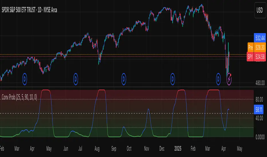
Quarterly Theory ICT 03 [TradingFinder] Precision Swing Points🔵 Introduction
Precision Swing Point (PSP) is a divergence pattern in the closing of candles between two correlated assets, which can indicate a potential trend reversal. This structure appears at market turning points and highlights discrepancies between the price behavior of two related assets.
PSP typically forms in key timeframes such as 5-minute, 15-minute, and 90-minute charts, and is often used in combination with Smart Money Concepts (SMT) to confirm trade entries.
PSP is categorized into Bearish PSP and Bullish PSP :
Bearish PSP : Occurs when an asset breaks its previous high, and its middle candle closes bullish, while the correlated asset closes bearish at the same level. This divergence signals weakness in the uptrend and a potential price reversal downward.
Bullish PSP : Occurs when an asset breaks its previous low, and its middle candle closes bearish, while the correlated asset closes bullish at the same level. This suggests weakness in the downtrend and a potential price increase.
🟣 Trading Strategies Using Precision Swing Point (PSP)
PSP can be integrated into various trading strategies to improve entry accuracy and filter out false signals. One common method is combining PSP with SMT (divergence between correlated assets), where traders identify divergence and enter a trade only after PSP confirms the move.
Additionally, PSP can act as a liquidity gap, meaning that price tends to react to the wick of the PSP candle, making it a favorable entry point with a tight stop-loss and high risk-to-reward ratio. Furthermore, PSP combined with Order Blocks and Fair Value Gaps in higher timeframes allows traders to identify stronger reversal zones.
In lower timeframes, such as 5-minute or 15-minute charts, PSP can serve as a confirmation for more precise entries in the direction of the higher timeframe trend. This is particularly useful in scalping and intraday trading, helping traders execute smarter entries while minimizing unnecessary stop-outs.
🔵 How to Use
PSP is a trading pattern based on divergence in candle closures between two correlated assets. This divergence signals a difference in trend strength and can be used to identify precise market turning points. PSP is divided into Bullish PSP and Bearish PSP, each applicable for long and short trades.
🟣 Bullish PSP
A Bullish PSP forms when, at a market turning point, the middle candle of one asset closes bearish while the correlated asset closes bullish. This discrepancy indicates weakness in the downtrend and a potential price reversal upward.
Traders can use this as a signal for long (buy) trades. The best approach is to wait for price to return to the wick of the PSP candle, as this area typically acts as a liquidity level.
f PSP forms within an Order Block or Fair Value Gap in a higher timeframe, its reliability increases, allowing for entries with tight stop-loss and optimal risk-to-reward ratios.
🟣 Bearish PSP
A Bearish PSP forms when, at a market turning point, the middle candle of one asset closes bullish while the correlated asset closes bearish. This indicates weakness in the uptrend and a potential price decline.
Traders use this pattern to enter short (sell) trades. The best entry occurs when price retests the wick of the PSP candle, as this level often acts as a resistance zone, pushing price lower.
If PSP aligns with a significant liquidity area or Order Block in a higher timeframe, traders can enter with greater confidence and place their stop-loss just above the PSP wick.
Overall, PSP is a highly effective tool for filtering false signals and improving trade entry precision. Combining PSP with SMT, Order Blocks, and Fair Value Gaps across multiple timeframes allows traders to execute higher-accuracy trades with lower risk.
🔵 Settings
Mode :
2 Symbol : Identifies PSP and PCP between two correlated assets.
3 Symbol : Compares three assets to detect more complex divergences and stronger confirmation signals.
Second Symbol : The second asset used in PSP and correlation calculations.
Third Symbol : Used in three-symbol mode for deeper PSP and PCP analysis.
Filter Precision X Point : Enables or disables filtering for more precise PSP and PCP detection. This filter only identifies PSP and PCP when the base asset's candle qualifies as a Pin Bar.
Trend Effect : By changing the Trend Effect status to "Off," all Pin bars, whether bullish or bearish, are displayed regardless of the current market trend. If the status remains "On," only Pin bars in the direction of the main market trend are shown.
Bullish Pin Bar Setting : Using the "Ratio Lower Shadow to Body" and "Ratio Lower Shadow to Higher Shadow" settings, you can customize your bullish Pin bar candles. Larger numbers impose stricter conditions for identifying bullish Pin bars.
Bearish Pin Bar Setting : Using the "Ratio Higher Shadow to Body" and "Ratio Higher Shadow to Lower Shadow" settings, you can customize your bearish Pin bar candles. Larger numbers impose stricter conditions for identifying bearish Pin bars.
🔵 Conclusion
Precision Swing Point (PSP) is a powerful analytical tool in Smart Money trading strategies, helping traders identify precise market turning points by detecting divergences in candle closures between correlated assets. PSP is classified into Bullish PSP and Bearish PSP, each playing a crucial role in detecting trend weaknesses and determining optimal entry points for long and short trades.
Using the PSP wick as a key liquidity level, integrating it with SMT, Order Blocks, and Fair Value Gaps, and analyzing higher timeframes are effective techniques to enhance trade entries. Ultimately, PSP serves as a complementary tool for improving entry accuracy and reducing unnecessary stop-outs, making it a valuable addition to Smart Money trading methodologies.
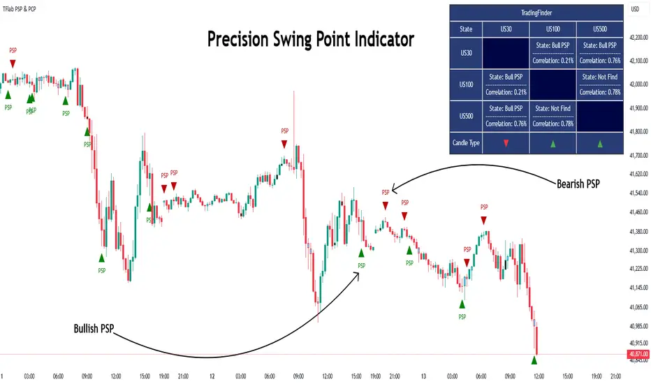
Finite Difference - Backward (mcbw_)In calculus there exists a 'derivative', which simply just measures the difference between two points on a curve. For well behaved mathematical functions there are infinitely many points and so there exists a derivative at every point. Where there are infinitely many points in a curve that curve is called 'continuous'. Continuous curves are very nice to deal with since each point on it exists almost exactly where its neighbors are. However, if the curve does not have infinitely many points on it, but instead has a finite number of points on it, that curve is called 'discrete' instead of continuous. Taking the derivative of discrete curves is much trickier business since there are none of the mathematical conveniences that a continuous offers. In the real world everything we measure is a discrete curve, including Price (since we measure it a finite number of times, aka each candlestick)!
The branch of Discrete Mathematics has found an approach to measure the derivative along a discrete curve, that approach is aptly called " Finite Difference ". To get a more accurate approximation of a discrete derivative, the finite difference approach uses weighted combinations of neighboring points. The most common type of finite difference is a 'central' difference, this uses a combination of points before and after the point of interest to approximate the discrete derivative. This is great for historical analysis but is not of much use for trading algorithms since it technically means using future prices to calculate the derivative of the current point. Instead we can use a less common variant called a ' Backwards Difference ' that only uses a combination of points before the current one to help approximate the current derivative.
In this script you can choose the " Order " of your derivative and the " Accuracy " of its approximation. This script is for educational purposes for folks building trading algorithms. Many trading algorithms often have an element of seeing how much Price has changed from the previous candle to the current candle. This approach is the lowest accuracy derivative possible, and using the backwards finite differences, made available for the first time on TradingView (!!), algorithms that use derivatives can now have higher orders of accuracy!
Happy Trading/Developing!
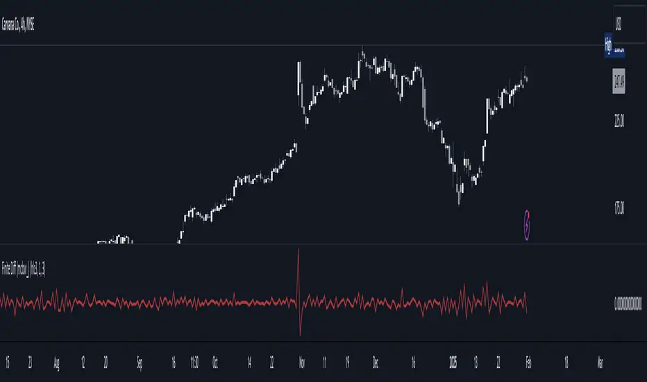
Dynamic Customizable 50% Line & Daily High/Low + True Day OpenA Unique Indicator for Precise Market-Level Analysis
This indicator is a fully integrated solution that automates complex market-level calculations and visualizations, offering traders a tool that goes beyond the functionality of existing open-source alternatives. By seamlessly combining several trading concepts into a single script, it delivers efficiency, accuracy, and customization that cater to both novice and professional traders.
Key Features: A Breakdown of What Makes It Unique
1. Adaptive Daily Highs and Lows
Automatically detects and plots daily high and low levels based on the selected time frame, dynamically updating in real time.
Features session-based adjustments, allowing traders to focus on levels that matter for specific trading sessions (e.g., London, New York).
Fully customizable styling, visibility, and alerts tailored to each trader’s preferences.
How It Works:
The indicator calculates daily high and low levels directly from price data, integrating session-specific time offsets to account for global trading hours. These levels provide traders with clear visual markers for key liquidity zones.
2. Automated ICT 50% Range Line
A pioneering implementation of ICT’s mid-range concept, this feature dynamically calculates and displays the midpoint of the daily range.
Offers traders a visual guide to identify premium and discount zones, aiding in determining market bias and potential trade setups.
How It Works:
The script calculates the range between the day’s high and low, dividing it by two to generate the midline. This line updates in real-time, ensuring that traders always see the most current premium and discount levels as price action evolves.
3. Dynamic Market Open Levels
Plots session opens (e.g., Asia, London, New York) and the True Day Open to provide actionable reference points for intra-day trading strategies.
Enhances precision in identifying liquidity shifts and aligning trades with institutional price movements.
How It Works:
The indicator uses predefined session times to calculate and display the opening levels for key trading sessions. It dynamically adjusts for time zones, ensuring accuracy regardless of the trader’s location.
4. Custom Watermark for Enhanced Visualization
Includes an optional watermark feature that allows users to display custom text on their charts.
Ideal for personalization, branding, or highlighting session notes without disrupting the clarity of the chart.
Why This Indicator Stands Out
First-to-Market Automation:
While the ICT 50% range line is a widely recognized concept, this is the first script to automate its calculation, combining it with other pivotal trading levels in a single tool.
All-in-One Functionality:
Unlike open-source alternatives that focus on individual features, this script integrates daily highs/lows, mid-range levels, session opens, and customizable watermarks into one cohesive system. The consolidation reduces the need for multiple indicators and ensures a clean, efficient chart setup.
Dynamic Customization:
Every feature can be adjusted to align with a trader’s strategy, time zone, or aesthetic preferences. This level of adaptability is unmatched in existing tools.
Proprietary Logic:
The indicator’s underlying calculations are built from scratch, leveraging advanced programming techniques to ensure accuracy and reliability. These proprietary methods differentiate it from similar open-source scripts.
How to Use This Indicator
Apply the Indicator:
Add it to your TradingView chart from the library.
Configure Settings:
Use the intuitive settings panel to adjust plotted levels, colors, styles, and visibility. Tailor the indicator to your trading strategy.
Incorporate into Analysis:
Combine the plotted levels with your preferred trading approach to identify liquidity zones, establish market bias, and pinpoint potential reversals or entries.
Stay Focused:
With all key levels automated and updated in real time, traders can focus on execution rather than manual plotting.
Originality and Justification for Closed Source
This script is closed-source due to its unique combination of features and proprietary logic that automates complex trading concepts like the ICT 50% range line and session-specific levels. Open-source alternatives lack this level of integration and customization, making this indicator a valuable and original contribution to the TradingView ecosystem.
What Sets It Apart from Open-Source Scripts?
Unlike open-source tools, this indicator doesn’t just replicate individual features—it enhances and integrates them into a seamless, all-in-one solution that offers traders a more efficient and effective way to analyze the market.
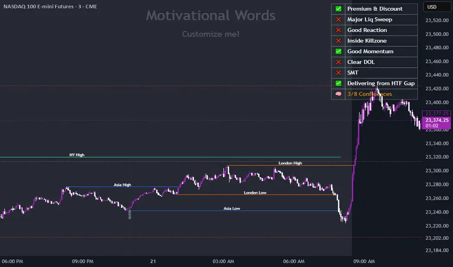
Fair Value Gap (FVG) Oscillator [UAlgo]The "Fair Value Gap (FVG) Oscillator " is designed to identify and visualize Fair Value Gaps (FVG) within a given lookback period on a trading chart. This indicator helps traders by highlighting areas where price gaps may signify potential trading opportunities, specifically bullish and bearish patterns. By leveraging volume and Average True Range (ATR) data, the FVG Oscillator aims to enhance the accuracy of pattern recognition and provide more reliable signals for trading decisions.
🔶 Identification of Fair Value Gap (FVG)
Fair Value Gaps (FVG) are specific price areas where gaps occur, and they are often considered significant in technical analysis. These gaps can indicate potential future price movements as the market may return to fill these gaps. This indicator identifies two types of FVGs:
Bullish FVG: Occurs when the current low price is higher than the high price two periods ago. This condition suggests a potential upward price movement.
Obtains with:
low > high
Bearish FVG: Occurs when the current high price is lower than the low price two periods ago. This condition suggests a potential downward price movement.
Obtains with:
high < low
The FVG Oscillator not only identifies these gaps but also verifies them using volume and ATR conditions to ensure more reliable trading signals.
🔶 Key Features
Lookback Period: Users can set the lookback period to determine how far back the indicator should search for FVG patterns.
ATR Multiplier: The ATR Multiplier is used to adjust the sensitivity of the ATR-based conditions for verifying FVG patterns.
Volume SMA Period: This setting determines the period for the Simple Moving Average (SMA) of the volume, which helps in identifying high volume conditions.
Why ATR and Volume are Used?
ATR (Average True Range) and volume are integrated into the Fair Value Gap (FVG) Oscillator to enhance the accuracy and reliability of the identified patterns. ATR measures market volatility, helping to filter out insignificant price gaps and focus on impactful ones, ensuring that the signals are relevant and strong. Volume, on the other hand, confirms the strength of price movements. High volume often indicates the sustainability of these movements, reducing the likelihood of false signals. Together, ATR and volume ensure that the detected FVGs are both significant and supported by market activity, providing more trustworthy trading signals.
Normalized Values: The FVG counts are normalized to enhance the visual representation and interpretation of the patterns on the chart.
Visual Customization and Plotting: Users can customize the colors for positive (bullish) and negative (bearish) areas, and choose whether to display these areas on the chart, also plots the bullish and bearish FVG counts, a zero line, and the net value of FVG counts. Additionally, it uses histograms to display the width of verified bullish and bearish patterns.
🔶 Disclaimer:
Use with Caution: This indicator is provided for educational and informational purposes only and should not be considered as financial advice. Users should exercise caution and perform their own analysis before making trading decisions based on the indicator's signals.
Not Financial Advice: The information provided by this indicator does not constitute financial advice, and the creator (UAlgo) shall not be held responsible for any trading losses incurred as a result of using this indicator.
Backtesting Recommended: Traders are encouraged to backtest the indicator thoroughly on historical data before using it in live trading to assess its performance and suitability for their trading strategies.
Risk Management: Trading involves inherent risks, and users should implement proper risk management strategies, including but not limited to stop-loss orders and position sizing, to mitigate potential losses.
No Guarantees: The accuracy and reliability of the indicator's signals cannot be guaranteed, as they are based on historical price data and past performance may not be indicative of future results.
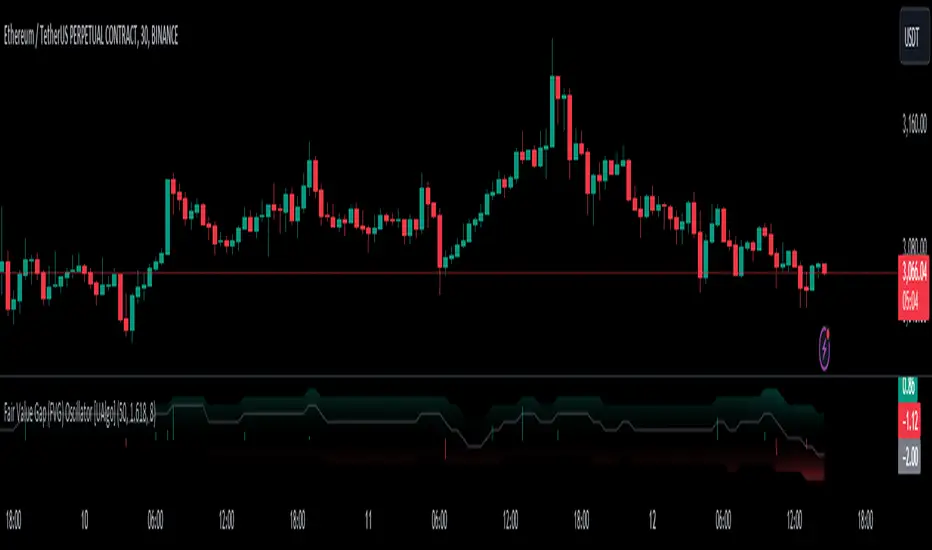
Alpha Trend IndicatorThe Alpha Trend Indicator is a custom-built trend-following tool designed to help traders identify market direction, trend strength, and potential reversal points with high accuracy. It combines multiple technical concepts—ATR (Average True Range), CCI (Commodity Channel Index), and either MFI (Money Flow Index) or RSI (Relative Strength Index)—to create a dynamic trend detection system.
🔑 Key Features:
Adaptive Trend Line – Uses ATR and CCI logic (similar to Trend Magic) to plot an Alpha Trend line that adjusts to volatility.
MFI / RSI Flexibility – Option to switch between MFI (volume-based momentum) or RSI (price-based momentum) for more tailored analysis.
Alpha Trend Offset – Plots a 2-bar shifted reference line to detect changes in price momentum.
Buy & Sell Signals – Automatically detects bullish and bearish crossovers between Alpha Trend and its offset line, marking potential entries and exits.
Visual Trend Zones – Fills the space between Alpha Trend and its offset with green (bullish) or red (bearish) highlights, making trend direction easy to see at a glance.
Alerts – Built-in alert conditions for Buy and Sell signals so traders never miss an opportunity.
📊 How It Works:
Trend Detection –
When CCI > 0, the Alpha Trend line is set below recent lows minus volatility (ATR).
When CCI < 0, it shifts above recent highs plus volatility.
Momentum Confirmation –
MFI/RSI adds an extra confirmation layer to avoid false signals.
Trading Signals –
Buy Signal: When Alpha Trend crosses above its offset line.
Sell Signal: When Alpha Trend crosses below its offset line.
⚡ Best Use:
Works on all timeframes (scalping, swing trading, long-term analysis).
Suitable for Forex, Crypto, Stocks, and Commodities.
Can be combined with support/resistance or volume analysis for even stronger setups.
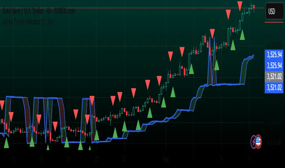
AlphaTrend Pro — Trend & Momentum Indicator📌 AlphaTrend Pro — Trend & Momentum Indicator
The AlphaTrend Pro is a professional trend-following & momentum confirmation tool designed to identify high-probability buy and sell signals in any market (Forex, Crypto, Indices, Commodities).
🔎 How It Works
AlphaTrend Bands (EMA ± ATR):
Dynamic support/resistance zones based on volatility.
Trend Detection:
✅ Price above Alpha Upper Band → Bullish Trend (BUY Zone).
❌ Price below Alpha Lower Band → Bearish Trend (SELL Zone).
⚪ Price between bands → Neutral (No Trade).
RSI Filter (Optional):
Prevents false entries in ranging markets.
Confirms momentum before signals.
📊 Features
Clear BUY/SELL signals with arrows on chart.
Trend-colored candles for quick visual bias.
Built-in alerts for automation (works with bots, Telegram, webhooks).
On-screen dashboard showing live trend status.
Works on all timeframes & markets (Scalping, Swing, Position Trading).
⚡ Best Use
Use on higher timeframes (1H, 4H, Daily) for trend confirmation.
Enter on lower timeframes for precise entries.
Combine with price action or support/resistance for maximum accuracy.

CVD Spaghetti - Multi-Exchange (Perpetuals)CVD Spaghetti – Multi-Exchange (Perpetuals) is designed to track and visualize Cumulative Volume Delta (CVD) across multiple cryptocurrency perpetual futures exchanges in one consolidated view. This indicator provides traders with a clearer perspective on buying and selling pressure by monitoring how order flow develops on different venues simultaneously.
What it does
The script calculates the CVD for each enabled exchange and plots them as separate lines on a single chart, creating a “spaghetti” style visualization. This allows traders to identify relative strength or weakness between major exchanges, which can often hint at institutional positioning, liquidity shifts, and potential market imbalances.
Why it’s useful
Order flow and liquidity dynamics can differ significantly between exchanges. By aggregating and comparing these flows, traders can:
Detect which venue is leading during trend development.
Spot divergences between exchanges, which may indicate inefficiencies or arbitrage-driven movements.
Gauge overall sentiment strength by comparing multiple sources instead of relying on a single dataset.
Technical details
Anchor Period Reset: The cumulative calculation resets based on the user-defined Anchor Period (default: daily), keeping data relevant for the chosen trading horizon.
Dynamic Resolution: The script automatically selects an appropriate lower timeframe for data requests based on the chart timeframe to maintain responsiveness and accuracy.
Normalization: Not all exchanges report volume in the same way—some use quote currency (USD), others in contracts or ticks. To ensure comparability, this indicator normalizes volumes where necessary:
Bybit USD and OKX contracts are divided by price to approximate base-coin terms.
Single-contract venues (e.g., Deribit) are normalized similarly.
Exchanges already reporting in the base currency remain unchanged.
Multi-Exchange Coverage: Supports major venues including Binance, Bybit, OKX, Bitget, Coinbase, and optional secondary exchanges like Blofin, Whitebit, and Deribit.
Visual Aids:
Zero baseline for directional reference.
Vertical session markers at each reset point.
Optional exchange labels positioned dynamically on the last bar for quick identification.
How traders might use it
Trend confirmation: Strong synchronized CVD across all major exchanges supports continuation; fragmentation may suggest weakening conviction.
Cross-exchange divergence: When one exchange’s CVD diverges from others, it can signal localized liquidity shocks or large player activity.
High-frequency strategies: On lower timeframes, the spaghetti view can highlight which venue is absorbing or providing liquidity fastest, aiding short-term decision-making.

Hilly's Advanced Crypto Scalping Strategy - 5 Min ChartTo determine the "best" input parameters for the Advanced Crypto Scalping Strategy on a 5-minute chart, we need to consider the goals of optimizing for profitability, minimizing false signals, and adapting to the volatile nature of cryptocurrencies. The default parameters in the script are a starting point, but the optimal values depend on the specific cryptocurrency pair, market conditions, and your risk tolerance. Below, I'll provide recommended input values based on common practices in crypto scalping, along with reasoning for each parameter. I’ll also suggest how to fine-tune them using TradingView’s backtesting and optimization tools.
Recommended Input Parameters
These values are tailored for a 5-minute chart for liquid cryptocurrencies like BTC/USD or ETH/USD on exchanges like Binance or Coinbase. They aim to balance signal frequency and accuracy for day trading.
Fast EMA Length (emaFastLen): 9
Reasoning: A 9-period EMA is commonly used in scalping to capture short-term price movements while remaining sensitive to recent price action. It reacts faster than the default 10, aligning with the 5-minute timeframe.
Slow EMA Length (emaSlowLen): 21
Reasoning: A 21-period EMA provides a good balance for identifying the broader trend on a 5-minute chart. It’s slightly longer than the default 20 to reduce noise while confirming the trend direction.
RSI Length (rsiLen): 14
Reasoning: The default 14-period RSI is a standard choice for momentum analysis. It works well for detecting overbought/oversold conditions without being too sensitive on short timeframes.
RSI Overbought (rsiOverbought): 75
Reasoning: Raising the overbought threshold to 75 (from 70) reduces false sell signals in strong bullish trends, which are common in crypto markets.
RSI Oversold (rsiOversold): 25
Reasoning: Lowering the oversold threshold to 25 (from 30) filters out weaker buy signals, ensuring entries occur during stronger reversals.
MACD Fast Length (macdFast): 12
Reasoning: The default 12-period fast EMA for MACD is effective for capturing short-term momentum shifts in crypto, aligning with scalping goals.
MACD Slow Length (macdSlow): 26
Reasoning: The default 26-period slow EMA is a standard setting that works well for confirming momentum trends without lagging too much.
MACD Signal Smoothing (macdSignal): 9
Reasoning: The default 9-period signal line is widely used and provides a good balance for smoothing MACD crossovers on a 5-minute chart.
Bollinger Bands Length (bbLen): 20
Reasoning: The default 20-period Bollinger Bands are effective for identifying volatility breakouts, which are key for scalping in crypto markets.
Bollinger Bands Multiplier (bbMult): 2.0
Reasoning: A 2.0 multiplier is standard and captures most price action within the bands. Increasing it to 2.5 could reduce signals but improve accuracy in highly volatile markets.
Stop Loss % (slPerc): 0.8%
Reasoning: A tighter stop loss of 0.8% (from 1.0%) suits the high volatility of crypto, helping to limit losses on false breakouts while keeping risk manageable.
Take Profit % (tpPerc): 1.5%
Reasoning: A 1.5% take-profit target (from 2.0%) aligns with scalping’s goal of capturing small, frequent gains. Crypto markets often see quick reversals, so a smaller target increases the likelihood of hitting profits.
Use Candlestick Patterns (useCandlePatterns): True
Reasoning: Enabling candlestick patterns (e.g., engulfing, hammer) adds confirmation to signals, reducing false entries in choppy markets.
Use Volume Filter (useVolumeFilter): True
Reasoning: The volume filter ensures signals occur during high-volume breakouts, which are more likely to sustain in crypto markets.
Signal Arrow Size (signalSize): 2.0
Reasoning: Increasing the arrow size to 2.0 (from 1.5) makes buy/sell signals more visible on the chart, especially on smaller screens or volatile price action.
Background Highlight Transparency (bgTransparency): 85
Reasoning: A slightly higher transparency (85 from 80) keeps the background highlights subtle but visible, avoiding chart clutter.
How to Apply These Parameters
Copy the Script: Use the Pine Script provided in the previous response.
Paste in TradingView: Open TradingView, go to the Pine Editor, paste the code, and click "Add to Chart."
Set Parameters: In the strategy settings, manually input the recommended values above or adjust them via the input fields.
Test on a 5-Minute Chart: Apply the strategy to a liquid crypto pair (e.g., BTC/USDT, ETH/USDT) on a 5-minute chart.
Fine-Tuning for Optimal Performance
To find the absolute best parameters for your specific trading pair and market conditions, use TradingView’s Strategy Tester and optimization features:
Backtesting:
Run the strategy on historical data for your chosen pair (e.g., BTC/USDT on Binance).
Check metrics like Net Profit, Profit Factor, Win Rate, and Max Drawdown in the Strategy Tester.
Focus on a sample period of at least 1–3 months to capture various market conditions (bull, bear, sideways).
Parameter Optimization:
In the Strategy Tester, click the settings gear next to the strategy name.
Enable optimization for key inputs like emaFastLen (test range: 7–12), emaSlowLen (15–25), slPerc (0.5–1.5), and tpPerc (1.0–3.0).
Run the optimization to find the combination with the highest net profit or best Sharpe ratio, but avoid over-optimization (curve-fitting) by testing on out-of-sample data.
Market-Specific Adjustments:
Volatile Pairs (e.g., DOGE/USDT): Use tighter stop losses (e.g., 0.5–0.7%) and smaller take-profit targets (e.g., 1.0–1.2%) to account for rapid price swings.
Stable Pairs (e.g., BTC/USDT): Slightly wider stop losses (e.g., 1.0–1.2%) and take-profit targets (e.g., 1.8–2.5%) may work better.
Trending Markets: Increase emaSlowLen (e.g., to 25–30) to follow stronger trends.
Choppy Markets: Tighten bbMult (e.g., to 1.8) and lower rsiOverbought/rsiOversold (e.g., to 70/30) to filter noise.
Forward Testing:
After backtesting, run the strategy in real-time on a demo account for 1–2 weeks to validate performance under current market conditions.
Important Notes
No Universal "Best" Numbers: Optimal parameters vary by crypto pair, exchange, and market conditions (e.g., bull vs. bear market). The suggested values are a starting point based on common scalping practices.
Risk Management: Never risk more than 1–2% of your account per trade. Adjust position sizing in TradingView’s strategy settings to align with your risk tolerance.
Market Volatility: Crypto markets are highly volatile. Test the strategy on your specific pair and adjust parameters if signals are too frequent or too rare.
Not Financial Advice: This is an educational tool. Backtest thoroughly and use a demo account before trading with real funds.
If you want me to generate a chart showing backtest performance for specific parameters or to tweak the script further (e.g., adding more indicators or adjusting signal logic), let me know!can you add clear buy ans sell signs above the candles in this codeTo add clear buy and sell signals above the candles in the provided Pine Script, I'll modify the existing code to include prominent text labels directly above (for sell signals) and below (for buy signals) the candles. These labels will be larger, color-coded, and positioned to avoid clutter, ensuring they are easily visible on the chart. The core strategy logic (EMA, RSI, MACD, Bollinger Bands, candlestick patterns, and volume filter) will remain unchanged, and I'll reuse the same artifact_id since this is an update to the previous script.AdvancedCryptoScalpingStrategy.pinex-pine

Greer Gap# Greer Gap Indicator (No mitigation: i.e. removing false signals)
## Summary
The **Greer Gap Indicator** identifies **Fair Value Gaps (FVGs)** and introduces specialized **Greer Bull Gaps (Blue)** and **Greer Bear Gaps (Orange)** to highlight high-probability trading opportunities. Unlike traditional FVG indicators, it avoids hindsight bias by not removing historical gaps based on future price action, ensuring transparency in signal accuracy. Built upon LuxAlgo’s FVG logic, it adds unique filtering: only the first Greer Gap after an opposite gap is plotted if its level (min for Bull, max for Bear) is not higher/lower than the previous Greer Gap of the same type, while all valid gaps are recorded for comparison. Traders can use these gaps as support/resistance or entry signals, customizable via timeframe, look back, and display options.
## Description
This indicator detects and displays **Fair Value Gaps (FVGs)** on the chart, with a focus on specialized **Greer Gaps**:
- **Bullish Gaps (Green)**: Areas where the low of the current candle is above the high of a previous candle (look back period), indicating potential upward momentum.
- **Bearish Gaps (Red)**: Areas where the high of the current candle is below the low of a previous candle, indicating potential downward momentum.
- **Greer Bull Gaps (Blue)**: A bullish gap that is above the latest bearish gap's max. Only the first such gap after a bearish gap is plotted if it meets criteria (not higher than the previous Greer Bull Gap's min), but all valid ones are recorded for comparison.
- **Greer Bear Gaps (Orange)**: A bearish gap that is below the latest bullish gap's min. Only the first such gap after a bullish gap is plotted if it meets criteria (not lower than the previous Greer Bear Gap's max), but all valid ones are recorded.
## How It Works
The script uses a dynamic look back period to detect FVGs. It maintains a record of all detected gaps and applies additional logic for Greer Gaps:
- **Greer Bull Gaps**: Checks if the new bullish gap's min is above the latest bearish gap's max. Plots only if it's the first since the last bearish gap and its min is <= previous Greer Bull min (or first one).
- **Greer Bear Gaps**: Checks if the new bearish gap's max is below the latest bullish gap's min. Plots only if it's the first since the last bullish gap and its max is >= previous Greer Bear max (or first one).
- **Resets**: A new bearish gap resets the Greer Bull Gap flag, and a new bullish gap resets the Greer Bear Gap flag.
## How to Use
- **Timeframe**: Set a higher timeframe (e.g., 'D' for daily) to detect gaps from that timeframe on the current chart.
- **Look back Period**: Adjust to change gap detection sensitivity (default: 34). Use 2 if you want to compare to LuxAlgo
- **Extend**: Controls how far right the gap boxes extend.
- **Show Options**: Toggle visibility of all bullish/bearish gaps or Greer Gaps.
- **Colors**: Customize colors for each gap type.
- **Application**: Use Greer Gaps as potential support/resistance levels or entry signals, but combine with other analysis for confirmation.
## Originality and Credits
This script is inspired by and builds upon the **"Fair Value Gap "** indicator by LuxAlgo (available on TradingView: ()).
**Credits**: Thanks to LuxAlgo for the core FVG detection logic.
**Significant Changes**:
- Added **Greer Bull and Bear Gap** logic for filtered, directional gaps with reset mechanisms.
- Introduced recording of all valid Greer Gaps without plotting all, to compare levels without hindsight bias.
- **No mitigation/removal of gaps**: Unlike LuxAlgo's approach, which mitigates (removes or alters) gaps based on future price action (e.g., when filled), this can create a hindsight bias where incorrect signals disappear over time. If a signal is used for a trade and later removed due to new data, it doesn't reflect real-time performance accurately. The Greer Gap avoids this by using gap comparisons to validate signals without altering historical boxes, ensuring transparency in when signals were right or wrong.