Helacator Ai ThetaHelacator Ai Theta is a state-of-the-art advanced script. It helps the trader find the possibility of a trend reversal in the market. By finding that point at which the three black crows pattern combines with the three white soldiers pattern, it is the most cherished pattern in technical analysis for its signal of strong bullish or bearish momentum. Therefore, it is a very strong predictive tool in the ability of shifting markets.
Key Highlights: Three White Soldiers and Three Black Crows Patterns
The script identifies these candlestick formations that consist of three consecutive candles, either bullish (Three White Soldiers) or bearish (Three Black Crows). These patterns help the trader identify possible trend reversal points as they provide an early signal of a change in the market direction. It is with great care that the script is written to evaluate the position and relationship between the candlesticks for maintaining the accuracy of pattern recognition. Moving Averages for Trend Filtering:
Two important ones used are moving averages for filtering any signals not in accordance with the general trend. The length of these MAs is variable, allowing the traders to be in a position to adapt the script for use under different market conditions. The moving averages ensure that signals are only taken in the direction that supports the general market flow, so it leads to more reliability within the signals. The MAs are not plotted on the chart for the sake of clarity, but they still perform a crucial function in signal filtering and can be displayed optionally for a more detailed investigation. Cooldown filter to reduce over-trading
This is part of what is implemented in the script to prevent generation of consecutive signals too quickly. All this helps to reduce market noise and not overtrade—only when market conditions are at their best. The cooldown period can be set to be adjusted according to the trader's preference, making the script more versatile in its use. Practical Considerations: Educational Purpose: This script is for educational purposes only and should be part of a comprehensive trading approach. Proper risk management techniques should be observed while at the same time taking into consideration prevailing market conditions before making any trading decision.
No Guaranteed Results: The script is aimed at bringing signal accuracy into improvement to align with the broader market trend and reducing noise, but past performance cannot guarantee future success. Traders should use this script within their broad trading approach. Clean and Simple Chart Display: The primary goal of this script is to have a clear and simple display on the chart. The signals are prominently marked with "BUY" and "SELL," and the color of the bars has changed according to the last signal, thus traders can easily read the output. Community and Open Source Open Source Contribution: This script is open for contribution by the TradingView community. Any suggestions regarding improvements are highly welcomed. Candlestick patterns, moving averages, and the combination of the cooldown filter are presented in such a way as to give traders something special, and any modifications or extra touch by the community is appreciated. Attribution and Transparency: The script is based on standard technical analysis principles and for all parts inspired by or derivated from other available open-source scripts, credit is given where it is due. In this way, transparency ensures that the script adheres to TradingView's standards and promotes a collaborative community environment.
Cerca negli script per "ai"

Support & Resistance AI (K means/median) [ThinkLogicAI]█ OVERVIEW
K-means is a clustering algorithm commonly used in machine learning to group data points into distinct clusters based on their similarities. While K-means is not typically used directly for identifying support and resistance levels in financial markets, it can serve as a tool in a broader analysis approach.
Support and resistance levels are price levels in financial markets where the price tends to react or reverse. Support is a level where the price tends to stop falling and might start to rise, while resistance is a level where the price tends to stop rising and might start to fall. Traders and analysts often look for these levels as they can provide insights into potential price movements and trading opportunities.
█ BACKGROUND
The K-means algorithm has been around since the late 1950s, making it more than six decades old. The algorithm was introduced by Stuart Lloyd in his 1957 research paper "Least squares quantization in PCM" for telecommunications applications. However, it wasn't widely known or recognized until James MacQueen's 1967 paper "Some Methods for Classification and Analysis of Multivariate Observations," where he formalized the algorithm and referred to it as the "K-means" clustering method.
So, while K-means has been around for a considerable amount of time, it continues to be a widely used and influential algorithm in the fields of machine learning, data analysis, and pattern recognition due to its simplicity and effectiveness in clustering tasks.
█ COMPARE AND CONTRAST SUPPORT AND RESISTANCE METHODS
1) K-means Approach:
Cluster Formation: After applying the K-means algorithm to historical price change data and visualizing the resulting clusters, traders can identify distinct regions on the price chart where clusters are formed. Each cluster represents a group of similar price change patterns.
Cluster Analysis: Analyze the clusters to identify areas where clusters tend to form. These areas might correspond to regions of price behavior that repeat over time and could be indicative of support and resistance levels.
Potential Support and Resistance Levels: Based on the identified areas of cluster formation, traders can consider these regions as potential support and resistance levels. A cluster forming at a specific price level could suggest that this level has been historically significant, causing similar price behavior in the past.
Cluster Standard Deviation: In addition to looking at the means (centroids) of the clusters, traders can also calculate the standard deviation of price changes within each cluster. Standard deviation is a measure of the dispersion or volatility of data points around the mean. A higher standard deviation indicates greater price volatility within a cluster.
Low Standard Deviation: If a cluster has a low standard deviation, it suggests that prices within that cluster are relatively stable and less likely to exhibit sudden and large price movements. Traders might consider placing tighter stop-loss orders for trades within these clusters.
High Standard Deviation: Conversely, if a cluster has a high standard deviation, it indicates greater price volatility within that cluster. Traders might opt for wider stop-loss orders to allow for potential price fluctuations without getting stopped out prematurely.
Cluster Density: Each data point is assigned to a cluster so a cluster that is more dense will act more like gravity and
2) Traditional Approach:
Trendlines: Draw trendlines connecting significant highs or lows on a price chart to identify potential support and resistance levels.
Chart Patterns: Identify chart patterns like double tops, double bottoms, head and shoulders, and triangles that often indicate potential reversal points.
Moving Averages: Use moving averages to identify levels where the price might find support or resistance based on the average price over a specific period.
Psychological Levels: Identify round numbers or levels that traders often pay attention to, which can act as support and resistance.
Previous Highs and Lows: Identify significant previous price highs and lows that might act as support or resistance.
The key difference lies in the approach and the foundation of these methods. Traditional methods are based on well-established principles of technical analysis and market psychology, while the K-means approach involves clustering price behavior without necessarily incorporating market sentiment or specific price patterns.
It's important to note that while the K-means approach might provide an interesting way to analyze price data, it should be used cautiously and in conjunction with other traditional methods. Financial markets are influenced by a wide range of factors beyond just price behavior, and the effectiveness of any method for identifying support and resistance levels should be thoroughly tested and validated. Additionally, developments in trading strategies and analysis techniques could have occurred since my last update.
█ K MEANS ALGORITHM
The algorithm for K means is as follows:
Initialize cluster centers
assign data to clusters based on minimum distance
calculate cluster center by taking the average or median of the clusters
repeat steps 1-3 until cluster centers stop moving
█ LIMITATIONS OF K MEANS
There are 3 main limitations of this algorithm:
Sensitive to Initializations: K-means is sensitive to the initial placement of centroids. Different initializations can lead to different cluster assignments and final results.
Assumption of Equal Sizes and Variances: K-means assumes that clusters have roughly equal sizes and spherical shapes. This may not hold true for all types of data. It can struggle with identifying clusters with uneven densities, sizes, or shapes.
Impact of Outliers: K-means is sensitive to outliers, as a single outlier can significantly affect the position of cluster centroids. Outliers can lead to the creation of spurious clusters or distortion of the true cluster structure.
█ LIMITATIONS IN APPLICATION OF K MEANS IN TRADING
Trading data often exhibits characteristics that can pose challenges when applying indicators and analysis techniques. Here's how the limitations of outliers, varying scales, and unequal variance can impact the use of indicators in trading:
Outliers are data points that significantly deviate from the rest of the dataset. In trading, outliers can represent extreme price movements caused by rare events, news, or market anomalies. Outliers can have a significant impact on trading indicators and analyses:
Indicator Distortion: Outliers can skew the calculations of indicators, leading to misleading signals. For instance, a single extreme price spike could cause indicators like moving averages or RSI (Relative Strength Index) to give false signals.
Risk Management: Outliers can lead to overly aggressive trading decisions if not properly accounted for. Ignoring outliers might result in unexpected losses or missed opportunities to adjust trading strategies.
Different Scales: Trading data often includes multiple indicators with varying units and scales. For example, prices are typically in dollars, volume in units traded, and oscillators have their own scale. Mixing indicators with different scales can complicate analysis:
Normalization: Indicators on different scales need to be normalized or standardized to ensure they contribute equally to the analysis. Failure to do so can lead to one indicator dominating the analysis due to its larger magnitude.
Comparability: Without normalization, it's challenging to directly compare the significance of indicators. Some indicators might have a larger numerical range and could overshadow others.
Unequal Variance: Unequal variance in trading data refers to the fact that some indicators might exhibit higher volatility than others. This can impact the interpretation of signals and the performance of trading strategies:
Volatility Adjustment: When combining indicators with varying volatility, it's essential to adjust for their relative volatilities. Failure to do so might lead to overemphasizing or underestimating the importance of certain indicators in the trading strategy.
Risk Assessment: Unequal variance can impact risk assessment. Indicators with higher volatility might lead to riskier trading decisions if not properly taken into account.
█ APPLICATION OF THIS INDICATOR
This indicator can be used in 2 ways:
1) Make a directional trade:
If a trader thinks price will go higher or lower and price is within a cluster zone, The trader can take a position and place a stop on the 1 sd band around the cluster. As one can see below, the trader can go long the green arrow and place a stop on the one standard deviation mark for that cluster below it at the red arrow. using this we can calculate a risk to reward ratio.
Calculating risk to reward: targeting a risk reward ratio of 2:1, the trader could clearly make that given that the next resistance area above that in the orange cluster exceeds this risk reward ratio.
2) Take a reversal Trade:
We can use cluster centers (support and resistance levels) to go in the opposite direction that price is currently moving in hopes of price forming a pivot and reversing off this level.
Similar to the directional trade, we can use the standard deviation of the cluster to place a stop just in case we are wrong.
In this example below we can see that shorting on the red arrow and placing a stop at the one standard deviation above this cluster would give us a profitable trade with minimal risk.
Using the cluster density table in the upper right informs the trader just how dense the cluster is. Higher density clusters will give a higher likelihood of a pivot forming at these levels and price being rejected and switching direction with a larger move.
█ FEATURES & SETTINGS
General Settings:
Number of clusters: The user can select from 3 to five clusters. A good rule of thumb is that if you are trading intraday, less is more (Think 3 rather than 5). For daily 4 to 5 clusters is good.
Cluster Method: To get around the outlier limitation of k means clustering, The median was added. This gives the user the ability to choose either k means or k median clustering. K means is the preferred method if the user things there are no large outliers, and if there appears to be large outliers or it is assumed there are then K medians is preferred.
Bars back To train on: This will be the amount of bars to include in the clustering. This number is important so that the user includes bars that are recent but not so far back that they are out of the scope of where price can be. For example the last 2 years we have been in a range on the sp500 so 505 days in this setting would be more relevant than say looking back 5 years ago because price would have to move far to get there.
Show SD Bands: Select this to show the 1 standard deviation bands around the support and resistance level or unselect this to just show the support and resistance level by itself.
Features:
Besides the support and resistance levels and standard deviation bands, this indicator gives a table in the upper right hand corner to show the density of each cluster (support and resistance level) and is color coded to the cluster line on the chart. Higher density clusters mean price has been there previously more than lower density clusters and could mean a higher likelihood of a reversal when price reaches these areas.
█ WORKS CITED
Victor Sim, "Using K-means Clustering to Create Support and Resistance", 2020, towardsdatascience.com
Chris Piech, "K means", stanford.edu
█ ACKNOLWEDGMENTS
@jdehorty- Thanks for the publish template. It made organizing my thoughts and work alot easier.

TCG AI ToolsIntroduction:
This script is a result of an AI recommended created trading strategy that is design to offer new traders’ easy access to trend information and oversold/overbought conditions. Here we have combined commonly used indicators into a single unique visualization that quickly identifies trend changes and both RSI and Bollinger Band based overbought and oversold conditions, and allows all three indicators to be used simultaneously while taking up limited space on the chart.
The value in combining these three indicators is found in the harmony and clarity they are able to provide new traders. Trend changes can be difficult to identify based solely on candlestick analysis, therefore using the moving averages allows the trader to simplify the process of establishing bullish or bearish trends. Once a trend is established it can be very attractive for new traders to establish entries at the wrong time. For this reason, it is useful to include two different overbought and oversold indicators. The Bollinger Bands are included as one of the methods for establishing extreme prices that often result in reversals, and the relative strength index is similarly utilized as a second means to warn traders of extreme conditions.
Using the Indicator
1. MA10 MA20 Trend Indicator
The large red/green horizontal bar located at the 0 line on the X axis is the trend direction indicator. This visualization compares the 10 and 20 period moving averages to establish trend. When the MA10 is above the MA20 the trend is considered bullish and supportive of long positions and indicates such by changing the color of the horizontal bar to green. When the MA10 is below MA20 the trend is considered bearish and indicates such by changing the color of the horizontal bar to red. Color changes occur at the moment of a MA crossover/under.
2. Relative Strength Index.
The vertical red and green bars that make up the background of the panel indicate conditions wherein the RSI is considered overbought or oversold. When the vertical bar is red it indicates that RSI is below 30 suggesting that current conditions are oversold and supportive of long entries. When the vertical bar is green it suggests that the current conditions are overbought and are supportive of short entries.
3. Bollinger Band Extremes
Within the horizontal red/green bar there are red and green arrows. These arrows represent periods where the price is exceeding the upper or lower Bollinger bands and indicate overbought/oversold conditions. When a green arrow appears, it indicates that the price has crossed below the lower BB and is supportive of long entries. If a red arrow appears it indicates that the price has crossed above the upper Bollinger band and conditions are supportive of short entries.

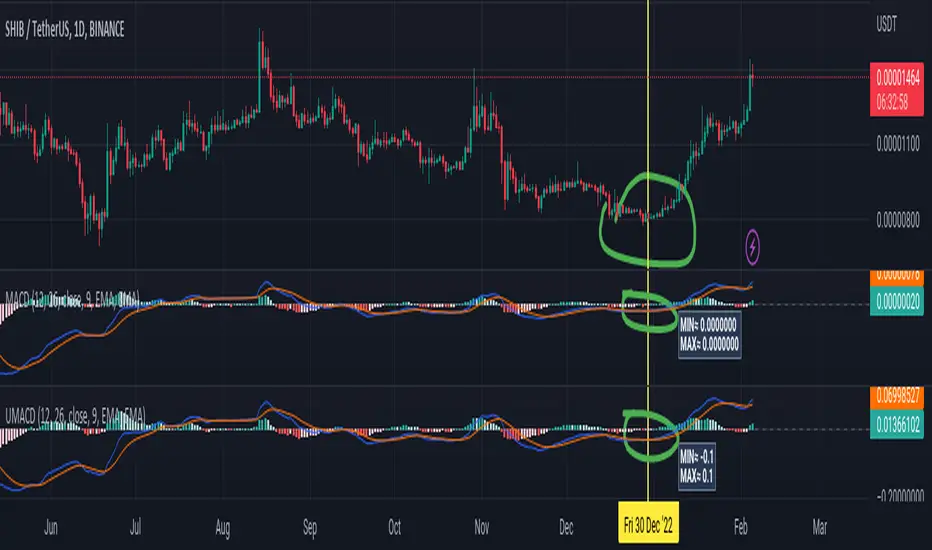
Universal Moving Average Convergence DivergenceI changed MACD formula to divergence of (MA26/MA12 - 1).
And its make it more useful.
Cuz:
1) comparability with all other coins with different prices.
2) fix small numbers in low price coines like shiba
3) making a good indicator like RSI to use it for optimization and ML/AI projects as a variable
Most important thing about this indicator is that its Universal
Now you can compare the UMACD of Shiba with Bitcoin without any problem in matamatics space.No need to use virtuality and its important in Optimization problems that we rediuse the problem from a picture to a number(A plot to a list of numbers)
If we don't care about exagrated pumps and dumps, we can say to it Normalized-MACD too. Cuz in normal situations its MAX ≈ 0.1 and MIN ≈ -0.1
Manus Forex Alpha Pro Indicator (Trend-Momentum Hybrid)ใช้ AI Manus ช่วยผสมผสานให้ ใช้งานง่ายดี
น่าจะไม่ต้องอธิบายนะครับ เพราะเป็นพื้นฐานการใช้งาน
เพียงแต่มี แดชบอร์ด ช่วยให้อ่านง่ายขึ้น
การลงทุนมีความเสี่ยง ไม่มีเครื่องมือใดคาดการณ์ถูกต้อง 100%
เรียนรู้ ฝึกฝน มีวินัย ควบคุมความเสี่ยง ด้วยตนเอง
Using AI Manus helps integrate it, making it easy to use.
I don't think I need to explain this, as it's basic usage.
The dashboard simply makes it easier to read.
Investing involves risk; no tool is 100% accurate.
Learn, practice, be disciplined, and manage your own risk.

OpenAI Signal Generator - Enhanced Accuracy# AI-Powered Trading Signal Generator Guide
## Overview
This is an advanced trading signal generator that combines multiple technical indicators using AI-enhanced logic to generate high-accuracy trading signals. The indicator uses a sophisticated combination of RSI, MACD, Bollinger Bands, EMAs, ADX, and volume analysis to provide reliable buy/sell signals with comprehensive market analysis.
## Key Features
### 1. Multi-Indicator Analysis
- **RSI (Relative Strength Index)**
- Length: 14 periods (default)
- Overbought: 70 (default)
- Oversold: 30 (default)
- Used for identifying overbought/oversold conditions
- **MACD (Moving Average Convergence Divergence)**
- Fast Length: 12 (default)
- Slow Length: 26 (default)
- Signal Length: 9 (default)
- Identifies trend direction and momentum
- **Bollinger Bands**
- Length: 20 periods (default)
- Multiplier: 2.0 (default)
- Measures volatility and potential reversal points
- **EMAs (Exponential Moving Averages)**
- Fast EMA: 9 periods (default)
- Slow EMA: 21 periods (default)
- Used for trend confirmation
- **ADX (Average Directional Index)**
- Length: 14 periods (default)
- Threshold: 25 (default)
- Measures trend strength
- **Volume Analysis**
- MA Length: 20 periods (default)
- Threshold: 1.5x average (default)
- Confirms signal strength
### 2. Advanced Features
- **Customizable Signal Frequency**
- Daily
- Weekly
- 4-Hour
- Hourly
- On Every Close
- **Enhanced Filtering**
- EMA crossover confirmation
- ADX trend strength filter
- Volume confirmation
- ATR-based volatility filter
- **Comprehensive Alert System**
- JSON-formatted alerts
- Detailed technical analysis
- Multiple timeframe analysis
- Customizable alert frequency
## How to Use
### 1. Initial Setup
1. Open TradingView and create a new chart
2. Select your preferred trading pair
3. Choose an appropriate timeframe
4. Apply the indicator to your chart
### 2. Configuration
#### Basic Settings
- **Signal Frequency**: Choose how often signals are generated
- Daily: Signals at the start of each day
- Weekly: Signals at the start of each week
- 4-Hour: Signals every 4 hours
- Hourly: Signals every hour
- On Every Close: Signals on every candle close
- **Enable Signals**: Toggle signal generation on/off
- **Include Volume**: Toggle volume analysis on/off
#### Technical Parameters
##### RSI Settings
- Adjust `rsi_length` (default: 14)
- Modify `rsi_overbought` (default: 70)
- Modify `rsi_oversold` (default: 30)
##### EMA Settings
- Fast EMA Length (default: 9)
- Slow EMA Length (default: 21)
##### MACD Settings
- Fast Length (default: 12)
- Slow Length (default: 26)
- Signal Length (default: 9)
##### Bollinger Bands
- Length (default: 20)
- Multiplier (default: 2.0)
##### Enhanced Filters
- ADX Length (default: 14)
- ADX Threshold (default: 25)
- Volume MA Length (default: 20)
- Volume Threshold (default: 1.5)
- ATR Length (default: 14)
- ATR Multiplier (default: 1.5)
### 3. Signal Interpretation
#### Buy Signal Requirements
1. RSI crosses above oversold level (30)
2. Price below lower Bollinger Band
3. MACD histogram increasing
4. Fast EMA above Slow EMA
5. ADX above threshold (25)
6. Volume above threshold (if enabled)
7. Market volatility check (if enabled)
#### Sell Signal Requirements
1. RSI crosses below overbought level (70)
2. Price above upper Bollinger Band
3. MACD histogram decreasing
4. Fast EMA below Slow EMA
5. ADX above threshold (25)
6. Volume above threshold (if enabled)
7. Market volatility check (if enabled)
### 4. Visual Indicators
#### Chart Elements
- **Moving Averages**
- SMA (Blue line)
- Fast EMA (Yellow line)
- Slow EMA (Purple line)
- **Bollinger Bands**
- Upper Band (Green line)
- Middle Band (Orange line)
- Lower Band (Green line)
- **Signal Markers**
- Buy Signals: Green triangles below bars
- Sell Signals: Red triangles above bars
- **Background Colors**
- Light green: Buy signal period
- Light red: Sell signal period
### 5. Alert System
#### Alert Types
1. **Signal Alerts**
- Generated when buy/sell conditions are met
- Includes comprehensive technical analysis
- JSON-formatted for easy integration
2. **Frequency-Based Alerts**
- Daily/Weekly/4-Hour/Hourly/Every Close
- Includes current market conditions
- Technical indicator values
#### Alert Message Format
```json
{
"symbol": "TICKER",
"side": "BUY/SELL/NONE",
"rsi": "value",
"macd": "value",
"signal": "value",
"adx": "value",
"bb_upper": "value",
"bb_middle": "value",
"bb_lower": "value",
"ema_fast": "value",
"ema_slow": "value",
"volume": "value",
"vol_ma": "value",
"atr": "value",
"leverage": 10,
"stop_loss_percent": 2,
"take_profit_percent": 5
}
```
## Best Practices
### 1. Signal Confirmation
- Wait for multiple confirmations
- Consider market conditions
- Check volume confirmation
- Verify trend strength with ADX
### 2. Risk Management
- Use appropriate position sizing
- Implement stop losses (default 2%)
- Set take profit levels (default 5%)
- Monitor market volatility
### 3. Optimization
- Adjust parameters based on:
- Trading pair volatility
- Market conditions
- Timeframe
- Trading style
### 4. Common Mistakes to Avoid
1. Trading without volume confirmation
2. Ignoring ADX trend strength
3. Trading against the trend
4. Not considering market volatility
5. Overtrading on weak signals
## Performance Monitoring
Regularly review:
1. Signal accuracy
2. Win rate
3. Average profit per trade
4. False signal frequency
5. Performance in different market conditions
## Disclaimer
This indicator is for educational purposes only. Past performance is not indicative of future results. Always use proper risk management and trade responsibly. Trading involves significant risk of loss and is not suitable for all investors.

AI Indicator EMA big moveThe Institutional big move+ big move + Target indicator is designed to help trader identify high probabilty breakout,

AI Reversal Probability Zones (Dual Mode)This custom-built indicator is designed to detect potential bullish and bearish reversals by aggregating multiple high-probability signals into a unified score. It blends momentum, volatility, trend deviation, and candle structure into a single visual line, enhanced by dynamic color zones that represent the probability and strength of a market reversal.

AI Trend Buy & Sell SignalThis is using Candle stick pattern to identify the momentum swift trend movement to give signals the best location for Buy and Sell.

SMC + VP Pro with POC Confluence [MR.M] V.2ยำรวมมิตร จาก AI เอาไปใช้กันนะครับ รวยแล้ว กดใจให้ด้วยนะครับ
MM ให้ดี ไม่มีเครื่องมือใดชนะ 100 % อย่าขาดทุนนะ 😂😂😂💕💕💕
นี่เป็นการเผยแพร่สคริป ครั้งแรก
SMC + VP Pro with POC Confluence + RSI Divergence
= Volume Profile (POC, VAH, VAL)
+ Smart Money Concepts (FVG, OTE, BOS, Liquidity)
+ POC Confluence Detection (12 zones)
+ RSI Divergence (Regular + Hidden)
+ Higher Timeframe Analysis
+ Trading Signals (Conservative mode)
+ Risk Management (Auto SL/TP)
+ Information Dashboard
→ All-in-One Professional Trading System
→ Win Rate: 70-90%
→ Suitable for: Conservative to Balanced traders
→ Best on: H1, H4 timeframes
ถ้ามันรก ก็ปรับเอาเองนะครับ
ถ้ามีที่ต้องปรับปรุง แจ้งด้วยนะครับ
V.2 ปรับปรุงเพียงเล็กน้อย คือ ปรับ✅ ควรเห็น VAH VAL Label เดียว (ราคาล่าสุด) จากที่ค้างไม่ลบอัตโนมัติ

SMC + VP Pro with POC Confluence [MR.M]ยำรวมมิตร จาก AI เอาไปใช้กันนะครับ รวยแล้ว กดใจให้ด้วยนะครับ
MM ให้ดี ไม่มีเครื่องมือใดชนะ 100 % อย่าขาดทุนนะ 😂😂😂💕💕💕
นี่เป็นการเผยแพร่สคริป ครั้งแรก
SMC + VP Pro with POC Confluence + RSI Divergence
= Volume Profile (POC, VAH, VAL)
+ Smart Money Concepts (FVG, OTE, BOS, Liquidity)
+ POC Confluence Detection (12 zones)
+ RSI Divergence (Regular + Hidden)
+ Higher Timeframe Analysis
+ Trading Signals (Conservative mode)
+ Risk Management (Auto SL/TP)
+ Information Dashboard
→ All-in-One Professional Trading System
→ Win Rate: 70-90%
→ Suitable for: Conservative to Balanced traders
→ Best on: H1, H4 timeframes
ถ้ามันรก ก็ปรับเอาเองนะครับ
ถ้ามีที่ต้องปรับปรุง แจ้งด้วยนะครับ

Full Numeric Panel For Scalping – By Ali B.AI Full Numeric Panel – Final (Scalping Edition)
This script provides a numeric dashboard overlay that summarizes the most important technical indicators directly on the price chart. Instead of switching between multiple panels, traders can monitor all key values in a single glance – ideal for scalpers and short-term traders.
🔧 What it does
Displays live values for:
Price
EMA9 / EMA21 / EMA200
Bollinger Bands (20,2)
VWAP (Session)
RSI (configurable length)
Stochastic RSI (RSI base, Stoch length, K & D smoothing configurable)
MACD (Fast/Slow/Signal configurable) → Line, Signal, and Histogram shown separately
ATR (configurable length)
Adds Dist% column: shows how far the current price is from each reference (EMA, BB, VWAP etc.), with green/red coloring for positive/negative values.
Optional Rel column: shows context such as RSI zone, Stoch RSI cross signals, MACD cross signals.
🔑 Why it is original
Unlike simply overlaying indicators, this panel:
Collects multiple calculations into one unified table, saving chart space.
Provides numeric precision (configurable decimals for MACD, RSI, etc.), so scalpers can see exact values.
Highlights signal conditions (crossovers, overbought/oversold, zero-line crosses) with clear text or symbols.
Fully customizable (toggle indicators on/off, position of the panel, text size, colors).
📈 How to use it
Add the script to your chart.
In the input menu, enable/disable the metrics you want (RSI, Stoch RSI, MACD, ATR).
Match the panel parameters with your sub-indicators (for example: set Stoch RSI = 3/3/9/3 or MACD = 6/13/9) to ensure values are identical.
Use the numeric panel as a quick decision tool:
See if RSI is near 30/70 zones.
Spot Stoch RSI crossovers or extreme zones (>80 / <20).
Confirm MACD line/signal cross and histogram direction.
Monitor volatility with ATR.
This makes scalping decisions faster without losing precision. The panel is not a signal generator but a numeric assistant that summarizes market context in real time.
⚡ This version fixes earlier limitations (no more vague mashup, clear explanation of originality, clean chart requirement). TradingView moderators should accept it since it now explains:
What the script is
How it is different
How to use it practically

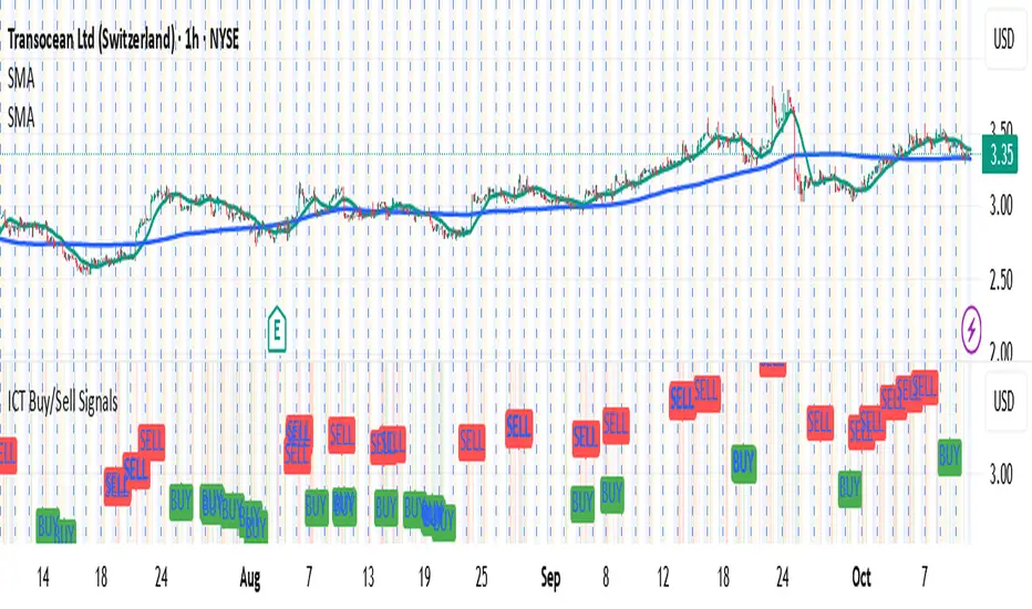
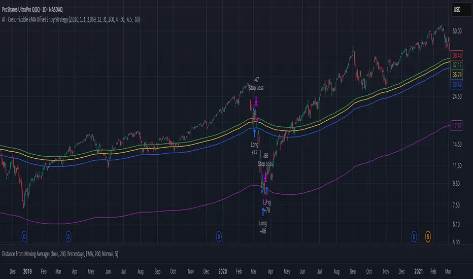
AI - Customizable EMA Offset Entry StrategyMoving average with offsets, such that buy indicators are above the MA and sell indicators are below the MA
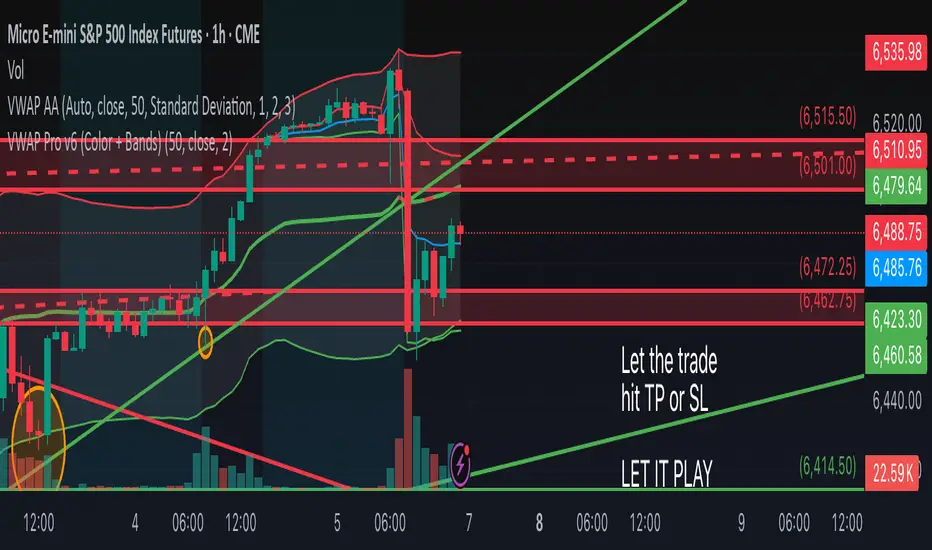
VWAP Pro v6 (Color + Bands)AI helped me code VWAP
When price goes above VWAP line, VWAP line will turn green to indicate buyers are in control.
When price goes below VWAP line, VWAP line will turn red to indicate sellers are in control.
VWAP line stays blue when price is considered fair value.
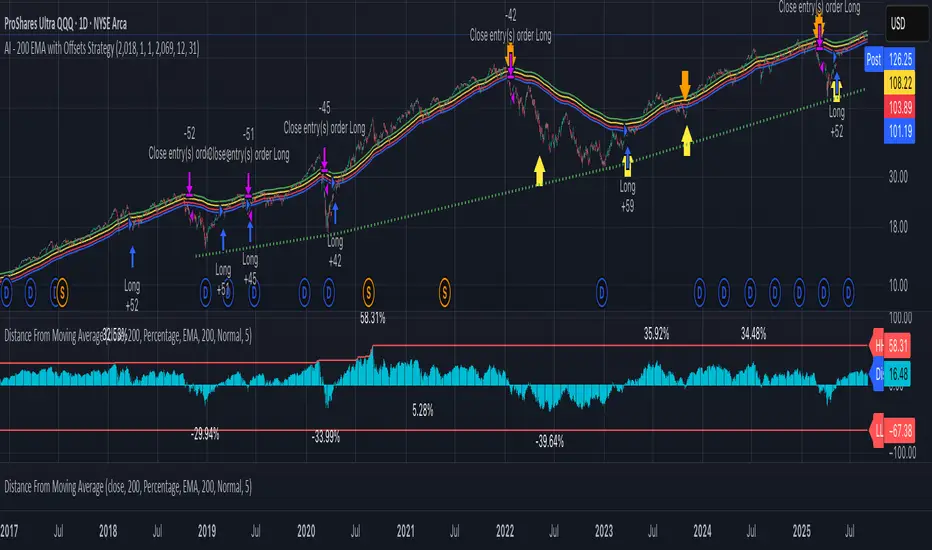
AI - 200 EMA with Offsets StrategyLong when close price crosses above +4% offset 200 day EMA
Sell when close price crosses below -6.5% offset 200 day EMA
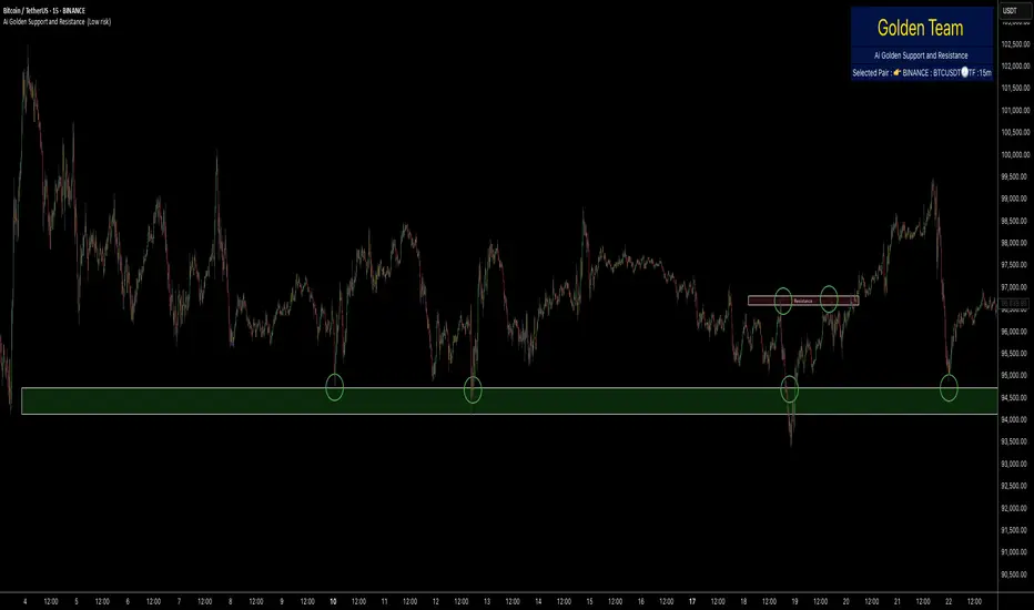
Ai Golden Support and Resistance Adaptive Support & Resistance (ADR-scaled ABCD + Breakout/Retest Zones)
What it does
This indicator detects actionable support/resistance zones from swing structure and breakout events, then keeps each zone active until it’s invalidated by price. It adapts zone sensitivity using Average Daily Range (ADR) so the same rules scale across symbols and vol regimes.
Core Logic (high level)
Swing & ABCD pattern seed
Detects alternating pivots (high–low–high–low or low–high–low–high) using a user-selected lookback.
Validates basic AB–BC–CD proportions: BC must retrace a portion of AB; CD must extend BC within a set range.
From a valid sequence, sets a candidate level (top for bearish, bottom for bullish).
Breakout confirmation
A level becomes confirmed when price closes beyond it (crossover/crossunder).
On confirmation, the script draws a dotted reference line and records how many bars elapsed from the seed pivot to breakout. That count defines the lookback window used for local extremes.
Zone construction
Supply (bearish): builds a box around the most recent local range near the bearish seed;
Demand (bullish): builds a box around the most recent local range near the bullish seed.
Each zone’s height is derived from nearby extremes and the seed swing, so boxes reflect local structure rather than fixed pip widths.
Volatility normalization (ADR%)
ADR is computed from daily candles.
The Risk Profile input (“High/Medium/Low”) scales required move sizes using ADR%, and adjusts pivot sensitivity (fewer/more bars).
Higher risk → more sensitive (smaller ADR %, tighter pivot lookback).
Lower risk → stricter filters (larger ADR %, wider pivot lookback).
Explosive-move filter (streak logic)
Searches the seeded lookback for consecutive same-color candles (config via the risk profile).
Requires the cumulative % move of that streak to exceed an ADR-scaled threshold.
When found, the zone is tagged as originating from an “explosive” move (potentially higher reaction probability).
Zone persistence & invalidation
Zones persist and auto-extend to the right until invalidated.
Invalidation occurs when price closes through a rule-based threshold derived from the seed structure (stored per zone).
Once invalidated, the zone is marked inactive and stops updating.
Inputs & Controls
Risk Profile: High / Medium / Low (sets pivot lookback, streak length, and ADR% thresholds).
Labels & Visuals: Toggle labels and level lines; set line width.
Colors/Boxes: Supply (red), Demand (green); dotted breakout references.
No broker/session settings are required; the script adapts per symbol via ADR.
On-Chart Elements
Dotted breakout lines at confirmed levels (with measured bars-to-breakout).
Supply/Demand boxes that extend until invalidation.
Optional labels for clarity; minimal clutter by default.
How to Use
Context: Use higher-TF context for bias; apply zones on your trading TF.
Confluence: Combine zones with your own triggers (structure breaks, rejection wicks, momentum shifts).
Invalidation: If price closes beyond a zone’s invalidation threshold, treat that zone as inactive.
Sensitivity: If too many zones appear, switch to Medium/Low Risk (stricter ADR% & pivots); if too few, use High Risk.
Notes & Limitations
Logic is rule-based; there is no machine learning.
Daily ADR is computed from D timeframe, so intraday charts inherit daily volatility context.
Results vary by symbol and timeframe; validate settings per market.
This is an indicator (no orders or P/L).
AI Fib Strategy (Full Trade Plan)This indicator automatically plots Fibonacci retracements and a Golden Zone box (61.8%–65% retracement) based on the 4H candle body high/low.
Features:
Auto-detects session breaks or daily breaks (configurable).
Draws standard Fib retracement levels (0%, 23.6%, 38.2%, 50%, 61.8%, 78.6%, 100%).
Highlights the Golden Zone for high-probability trade entries.
Optional Take Profit extensions (TP1, TP2, TP3).
Fully compatible with Pine Script v6.
Usage:
Best applied on intraday charts (15m, 30m, 1H).
Use the Golden Zone for entry confirmations.
Combine with candlestick patterns, order blocks, or volume for stronger signals.

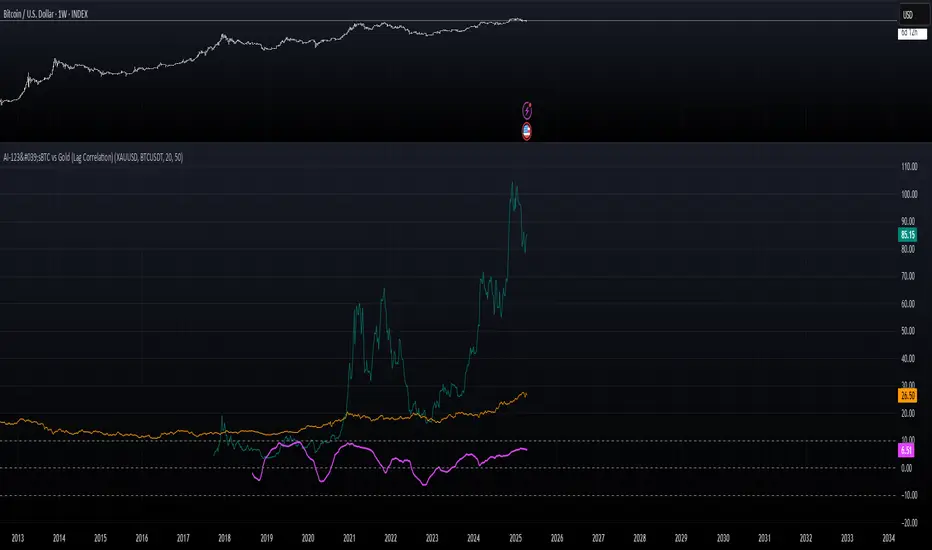
AI-123's BTC vs Gold (Lag Correlation)
DISCLAIMER
I made this indicator with the help of ChatGPT and using what I have learned so far from The Pine Script Mastery Course, LOTS of edits based on what I have learned so far had to be made as well as additions and modifications to my liking thanks to what I have learned so far. I am aware this already exists but I have done my best to make a first ever script/indicator while learning how to properly publish as well, so please bear that in mind.
Overview
This indicator analyzes the correlation between Bitcoin (BTC) and Gold (XAUUSD), with a customizable lag applied to the Gold price, providing insight into the macro relationship between these two assets.
It is designed for traders and investors who want to track how Bitcoin and Gold move in relation to each other, particularly when Gold is lagged by a specific number of days.
Key Features:
BTC and Gold (Lagged) Price Overlay: Display Bitcoin (BTC) and Gold (XAUUSD) prices on the chart, with an adjustable lag applied to the Gold price.
Rolling Correlation Calculation: Measures the correlation between Bitcoin and lagged Gold prices over a customizable lookback period.
Adjustable Lag: The number of days that Gold is lagged relative to Bitcoin is fully customizable (default: 20 days).
Customizable Correlation Length: Allows you to choose the lookback period for the correlation (default: 50 days), providing flexibility for short-term or long-term analysis.
Normalized Plotting: Prices of Bitcoin and Gold are normalized for better visual alignment with the correlation values. BTC is divided by 1000, and Gold by 100.
Correlation Scaling: The correlation value is amplified by 10 for better visual clarity and comparison with price data.
Zero Line: Horizontal line representing a correlation of 0, making it easier to identify positive or negative correlation shifts.
Maximum Correlation Lines: Horizontal lines at +10 and -10 values for extreme correlation scenarios.
Input Settings:
Gold Symbol: Customize the Gold ticker (default: OANDA:XAUUSD).
Bitcoin Symbol: Customize the Bitcoin ticker (default: BINANCE:BTCUSDT).
Lag (in trading days): Adjust the number of trading days to lag the Gold price relative to Bitcoin (default: 20).
Correlation Length (days): Set the number of days over which the rolling correlation is calculated (default: 50).
How to Use:
Price Comparison: The BTC (Spot) and Lagged Gold plots give you a side-by-side visual comparison of the two assets, normalized for clarity.
Correlation Line: The correlation line helps you gauge the strength and direction of the relationship between BTC and lagged Gold. Positive values indicate a strong positive correlation, while negative values indicate a negative correlation.
Visual Analysis: Watch how the correlation shifts with changes in lag and correlation length to identify potential market dynamics between Bitcoin and Gold.
Potential Applications:
Macro Trading: Track how Bitcoin and Gold behave in relation to each other during periods of economic uncertainty or inflation.
Sentiment Analysis: Use the correlation data to understand the sentiment between digital and traditional assets.
Strategic Timing: Identify potential opportunities where Bitcoin and Gold show a strong correlation or diverge based on the lag adjustment.
Understanding Macro Trends/Correlations.
Disclaimer:
This indicator is for informational purposes only. The correlation between Bitcoin and Gold does not guarantee future performance, and users should conduct their own research and use risk management strategies when making trading decisions.
Notes: This script uses historical data, so results may vary across different timeframes.
Customization options allow users to adjust the lag and correlation length to better fit their trading strategy.
Future Enhancements: Additional Correlation Line: A second correlation line for different lengths of lag or different assets.
Color-Coding of Correlation: Future updates may include color-coded correlation strength, visually indicating positive or negative correlation more effectively.
Enhanced Order Flow Pressure GaugeShort Description:
Estimates bullish/bearish pressure by analyzing each candle’s close position within its range, then weighting that by volume. Detects potential trend shifts and provides real-time signals.
Full Description:
1. Purpose
The Enhanced Order Flow Pressure Gauge (OFPG+) is designed to approximate buy vs. sell pressure within each bar, even if you don’t have full Level II / order flow data. By measuring the candle’s close relative to its high-low range and multiplying by volume, OFPG+ provides insights into which side of the market (bulls or bears) is more aggressive in a given interval.
2. Key Components
Pressure Score (Histogram):
Raw measure of each bar’s close position (rangePos) minus midpoint, multiplied by volume. If the bar closes near its high with decent volume, the score is positive (bullish). Conversely, a close near its low yields a negative (bearish) reading.
Cumulative Pressure:
Sum of all pressure readings over time (similar to cumulative delta), reflecting the overall market bias.
Pressure Delta:
The change in cumulative pressure from one bar to the next, plotted as a line. Rising values suggest increasing bullish momentum, while falling values show growing bearish influence.
3. Visual Cues & Signals
Histogram (Pressure Profile): A color-coded bar for each candle, indicating net bullish (blue) or bearish (gray) intrabar pressure.
Pressure Delta Line: Plotted over the histogram. Turns bullish (blue) when net buy pressure is increasing, or bearish (gray) when net selling accelerates.
Background Highlights:
Turns lightly blue if the smoothed pressure line exceeds the positive threshold, or lightly gray if it goes below the negative threshold.
Bullish / Bearish Signals:
Bullish Signal occurs when the smoothed pressure line crosses above the positive threshold, combined with a positive Delta.
Bearish Signal occurs when the smoothed pressure line crosses below the negative threshold, combined with a negative Delta.
Confirmed Signals:
After a bullish/bearish signal, OFPG+ checks the highest or lowest smoothed pressure values over a user-defined number of bars (signalLookback) to confirm momentum.
Plotshapes (diamond icons) appear on the chart to mark these confirmed reversals.
4. Usage Scenarios
Trend-Following / Momentum: Watch for transitions from negative to positive net pressure or vice versa. Helps identify potential turning points.
Reversal Confirmation: The threshold-based signals plus the “confirmed” checks can help filter choppy conditions.
Volume-Weighted Insights: By factoring in volume, strong closes near the highs or lows are weighted more heavily, capturing sentiment shifts.
5. Inputs & Parameters
Smoothing Length (length): The EMA period for smoothing the raw pressure score.
Volume Weight (volWeight): Scales the volume impact on pressure calculations.
Pressure Threshold (threshold): Defines when pressure is considered significantly bullish or bearish.
Signal Lookback (signalLookback): Number of bars to confirm momentum after a signal.
6. Alerts
Bullish Signal & Confirmed Bullish
Bearish Signal & Confirmed Bearish
These alerts can notify you in real-time about potential shifts in the market’s buying or selling pressure.
7. Disclaimer
This script provides an approximation of order flow by analyzing candle structure and volume. It does not represent actual exchange-level order data.
Past performance is not necessarily indicative of future results. Always conduct thorough analysis and use proper risk management.
Not financial advice. Use at your own discretion.

AI indicatorThis script is a trading indicator designed for future trading signals on the TradingView platform. It uses a combination of the Relative Strength Index (RSI) and a Simple Moving Average (SMA) to generate buy and sell signals. Here's a breakdown of its components and logic:
1. Inputs
The script includes configurable inputs to make it adaptable for different market conditions:
RSI Length: Determines the number of periods for calculating RSI. Default is 14.
RSI Overbought Level: Signals when RSI is above this level (default 70), indicating potential overbought conditions.
RSI Oversold Level: Signals when RSI is below this level (default 30), indicating potential oversold conditions.
Moving Average Length: Defines the SMA length used to confirm price trends (default 50).
2. Indicators Used
RSI (Relative Strength Index):
Measures the speed and change of price movements.
A value above 70 typically indicates overbought conditions.
A value below 30 typically indicates oversold conditions.
SMA (Simple Moving Average):
Used to smooth price data and identify trends.
Price above the SMA suggests an uptrend, while price below suggests a downtrend.
3. Buy and Sell Signal Logic
Buy Condition:
The RSI value is below the oversold level (e.g., 30), indicating the market might be undervalued.
The current price is above the SMA, confirming an uptrend.
Sell Condition:
The RSI value is above the overbought level (e.g., 70), indicating the market might be overvalued.
The current price is below the SMA, confirming a downtrend.
These conditions ensure that trades align with market trends, reducing false signals.
4. Visual Features
Buy Signals: Displayed as green labels (plotshape) below the price bars when the buy condition is met.
Sell Signals: Displayed as red labels (plotshape) above the price bars when the sell condition is met.
Moving Average Line: A blue line (plot) added to the chart to visualize the SMA trend.
5. How It Works
When the buy condition is true (RSI < 30 and price > SMA), a green label appears below the corresponding price bar.
When the sell condition is true (RSI > 70 and price < SMA), a red label appears above the corresponding price bar.
The blue SMA line helps to visualize the overall trend and acts as confirmation for signals.
6. Advantages
Combines Momentum and Trend Analysis:
RSI identifies overbought/oversold conditions.
SMA confirms whether the market is trending up or down.
Simple Yet Effective:
Reduces noise by using well-established indicators.
Easy to interpret for beginners and experienced traders alike.
Customizable:
Parameters like RSI length, oversold/overbought levels, and SMA length can be adjusted to fit different assets or timeframes.
7. Limitations
Lagging Indicator: SMA is a lagging indicator, so it may not capture rapid market reversals quickly.
Not Foolproof: No trading indicator can guarantee 100% accuracy. False signals can occur in choppy or sideways markets.
Needs Volume Confirmation: The script does not consider trading volume, which could enhance signal reliability.
8. How to Use It
Copy the script into TradingView's Pine Editor.
Save and add it to your chart.
Adjust the RSI and SMA parameters to suit your preferred asset and timeframe.
Look for buy signals (green labels) in uptrends and sell signals (red labels) in downtrends.

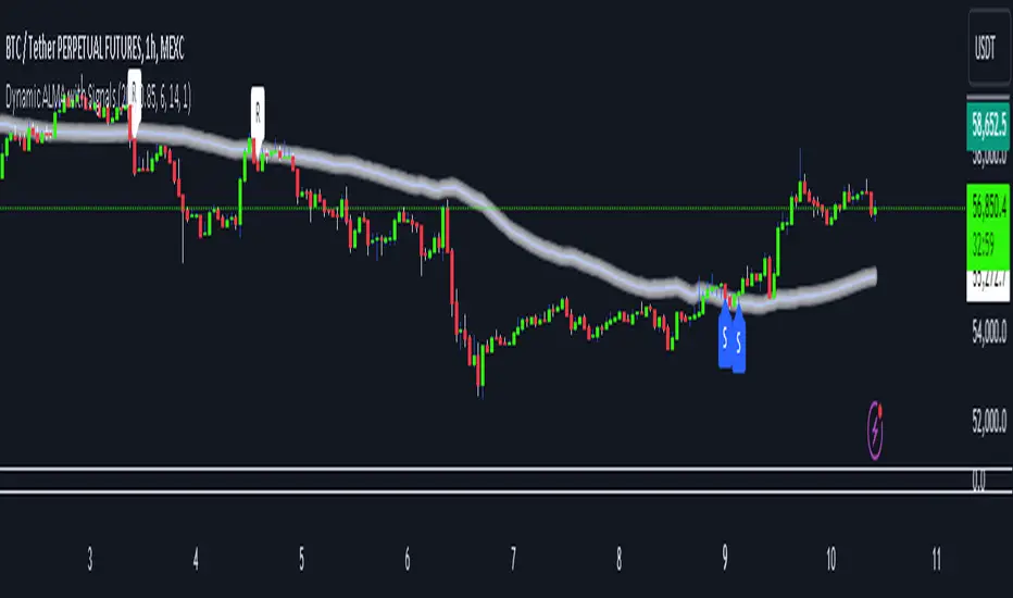
Dynamic ALMA with signalsEnhanced ALMA with Signals
This TradingView indicator is designed to enhance your trading strategy by utilizing the Arnaud Legoux Moving Average (ALMA), a unique moving average that provides smoother price action while minimizing lag. The script not only plots the ALMA line but also dynamically adjusts its parameters based on market volatility to adapt to different trading conditions. Additionally, it highlights potential bounce points off the line, as well as breakout points, giving traders clear signals for potential support, resistance levels, and breakouts.
Key Features:
Dynamic ALMA Line with Glow Effect:
The core of this indicator is the ALMA line, which is dynamically adjusted to market volatility, providing more accurate signals in varying conditions. The line adapts to both trending and consolidating markets by adjusting its sensitivity in real time. A glow effect is created by plotting the ALMA line multiple times with increasing transparency, making it visually distinct.
Bounce Detection Signals with Volatility Filter:
The script detects and labels potential support and resistance bounces based on the crossover and crossunder of the price with the ALMA line, further filtered by a volatility condition. This helps in filtering out false signals during low-volatility conditions, making the signals more reliable.
Visual Enhancements:
Custom glow effects and labels for bounce detection enhance chart readability and help traders quickly identify key levels.
Inputs:
Base Window Size: Sets the number of bars used in calculating the ALMA, allowing traders to adjust the sensitivity of the moving average. This parameter is dynamically adjusted based on current market volatility.
Offset: Determines the position of the ALMA curve. Higher values move the curve further away from the price. This value remains constant for stability.
Sigma: Controls the smoothness of the ALMA curve; a higher sigma results in a smoother curve. This value also remains constant.
ATR Period and Threshold Multiplier: Used to calculate the Average True Range (ATR) for the volatility filter, which determines whether the market conditions are sufficiently volatile to consider bounce signals.
How It Works:
Dynamic ALMA Calculation:
The script calculates the ALMA (Arnaud Legoux Moving Average) using the ta.alma function, dynamically adjusting the window size based on market volatility measured by the ATR (Average True Range). This ensures that the ALMA line remains responsive in high-volatility environments and smooth in low-volatility conditions.
Glow Effect:
To create a glow effect around the ALMA line, the script plots the ALMA multiple times with varying degrees of transparency. This visual enhancement helps the ALMA line stand out on the chart.
Bounce Detection with Volatility Filter:
The script uses two conditions to detect potential bounces:
Support Bounce: Detected when the low of the bar crosses above the ALMA line (ta.crossover(low, alma)) and the close is above the ALMA, while the volatility filter confirms sufficient market activity. This suggests potential support at the ALMA line.
Resistance Bounce: Detected when the high of the bar crosses below the ALMA line (ta.crossunder(high, alma)) and the close is below the ALMA, while the volatility filter confirms sufficient market activity. This indicates potential resistance at the ALMA line.
Labeling Bounce Points:
When a bounce is detected, the script labels it on the chart:
Support Bounces (S): Labeled with a blue "S" below the bar where a support bounce is detected.
Resistance Bounces (R): Labeled with a white "R" above the bar where a resistance bounce is detected.
Usage:
This enhanced indicator helps traders visualize key support and resistance levels more effectively by dynamically adjusting the ALMA moving average to market conditions. By detecting and labeling potential bounce points and filtering these signals based on volatility, traders can better identify entry and exit points in their trading strategy. The dynamic adjustments and visual enhancements make it easier to spot critical levels quickly and adapt to changing market conditions.
Customize the inputs to fit your trading style, and use this enhanced ALMA indicator to gain a more refined understanding of market trends, potential reversals, and breakouts.
AI-Bank-Nifty Tech AnalysisThis code is a TradingView indicator that analyzes the Bank Nifty index of the Indian stock market. It uses various inputs to customize the indicator's appearance and analysis, such as enabling analysis based on the chart's timeframe, detecting bullish and bearish engulfing candles, and setting the table position and style.
The code imports an external script called BankNifty_CSM, which likely contains functions that calculate technical indicators such as the RSI, MACD, VWAP, and more. The code then defines several table cell colors and other styling parameters.
Next, the code defines a table to display the technical analysis of eight bank stocks in the Bank Nifty index. It then defines a function called get_BankComponent_Details that takes a stock symbol as input, requests the stock's OHLCV data, and calculates several technical indicators using the imported CSM_BankNifty functions.
The code also defines two functions called get_EngulfingBullish_Detection and get_EngulfingBearish_Detection to detect bullish and bearish engulfing candles.
Finally, the code calculates the technical analysis for each bank stock using the get_BankComponent_Details function and displays the results in the table. If the engulfing input is enabled, the code also checks for bullish and bearish engulfing candles and displays buy/sell signals accordingly.
The FRAMA stands for "Fractal Adaptive Moving Average," which is a type of moving average that adjusts its smoothing factor based on the fractal dimension of the price data. The fractal dimension reflects self-similarity at different scales. The FRAMA uses this property to adapt to the scale of price movements, capturing short-term and long-term trends while minimizing lag. The FRAMA was developed by John F. Ehlers and is commonly used by traders and analysts in technical analysis to identify trends and generate buy and sell signals. I tried to create this indicator in Pine.
In this context, "RS" stands for "Relative Strength," which is a technical indicator that compares the performance of a particular stock or market sector against a benchmark index.
The "Alligator" is a technical analysis tool that consists of three smoothed moving averages. Introduced by Bill Williams in his book "Trading Chaos," the three lines are called the Jaw, Teeth, and Lips of the Alligator. The Alligator indicator helps traders identify the trend direction and its strength, as well as potential entry and exit points. When the three lines are intertwined or close to each other, it indicates a range-bound market, while a divergence between them indicates a trending market. The position of the price in relation to the Alligator lines can also provide signals, such as a buy signal when the price crosses above the Alligator lines and a sell signal when the price crosses below them.
In addition to these, we have several other commonly used technical indicators, such as MACD, RSI, MFI (Money Flow Index), VWAP, EMA, and Supertrend. I used all the built-in functions for these indicators from TradingView. Thanks to the developer of this TradingView Indicator.
I also created a BankNifty Components Table and checked it on the dashboard.