Aethix Cipher Pro2Aethix Cipher Pro: AI-Enhanced Crypto Signal Indicator grok Ai made signal created for aethix users.
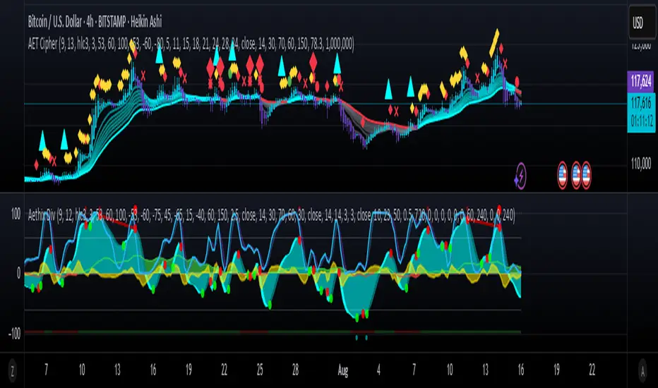
Unlock the future of crypto trading with Aethix Cipher Pro—a powerhouse indicator inspired by Market Cipher A, turbocharged for Aethix.io users! Built on WaveTrend Oscillator, 8-EMA Ribbon, RSI+MFI, and custom enhancements like Grok AI confidence levels (70-100%), on-chain whale volume thresholds, and fun meme alerts ("To the moon! 🌕").
Key Features:
WaveTrend Signals: Spot overbought/oversold with levels at ±53/60/100—crosses trigger red diamonds, blood diamonds, yellow X's for high-prob buy/sell entries.
Neon Teal EMA Ribbon: Dynamic 5-34 EMA gradient (bullish teal/bearish red) for trend direction—crossovers plot green/red circles, blue triangles.
RSI+MFI Fusion: Overbought (70+)/oversold (30-) with long snippets for sentiment edges.
Cerca negli script per "ai"
Aethix Cipher ProAethix Cipher Pro: AI-Enhanced Crypto Signal Indicator grok Ai made signal created for aethix users.
Unlock the future of crypto trading with Aethix Cipher Pro—a powerhouse indicator inspired by Market Cipher A, turbocharged for Aethix.io users! Built on WaveTrend Oscillator, 8-EMA Ribbon, RSI+MFI, and custom enhancements like Grok AI confidence levels (70-100%), on-chain whale volume thresholds, and fun meme alerts ("To the moon! 🌕").
Key Features:
WaveTrend Signals: Spot overbought/oversold with levels at ±53/60/100—crosses trigger red diamonds, blood diamonds, yellow X's for high-prob buy/sell entries.
Neon Teal EMA Ribbon: Dynamic 5-34 EMA gradient (bullish teal/bearish red) for trend direction—crossovers plot green/red circles, blue triangles.
RSI+MFI Fusion: Overbought (70+)/oversold (30-) with long snippets for sentiment edges.
CyberCandle SwiftEdgeCyberCandle SwiftEdge
Overview
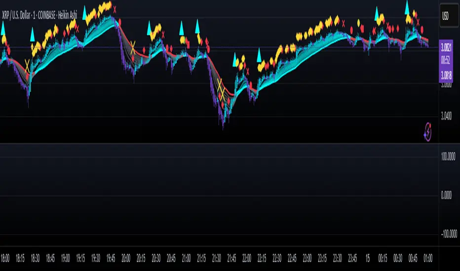
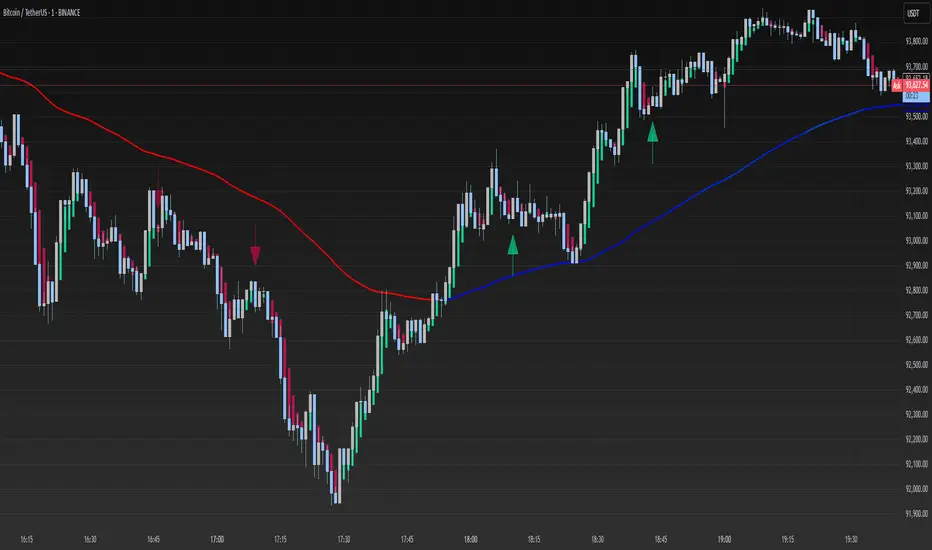
CyberCandle SwiftEdge is a cutting-edge, AI-inspired trading indicator designed for traders seeking precision and clarity in trend-following and swing trading. Powered by SwiftEdge, it combines Heikin Ashi candles, a gradient-colored Exponential Moving Average (EMA), and a Relative Strength Index (RSI) to deliver clear buy and sell signals. Featuring glowing visuals, dynamic signal icons, and a customizable RSI dashboard in the top-right corner, this script offers a futuristic interface for identifying high-probability trade setups on various timeframes (e.g., 1H, 4H).
What It Does
CyberCandle SwiftEdge integrates three powerful components to generate actionable trading signals:
Heikin Ashi Candles: Smooths price action to highlight trends, reducing market noise and making reversals easier to spot.
Gradient EMA: A 100-period EMA with dynamic color transitions (blue/cyan for uptrends, red/pink for downtrends) to confirm market direction.
RSI Dashboard: A neon-lit display showing RSI levels, indicating overbought (>70), oversold (<30), or neutral (30-70) conditions.
Buy and sell signals are marked with prominent, glowing icons (triangles and arrows) based on trend direction, momentum, and specific Heikin Ashi patterns. The script’s customizable parameters allow traders to tailor the strategy to their preferences, balancing signal frequency and precision.
How It Works
The strategy leverages the synergy of Heikin Ashi, EMA, and RSI to filter trades and highlight opportunities:
Trend Direction: The price must be above the EMA for buy signals (bullish trend) or below for sell signals (bearish trend). The EMA’s gradient color shifts based on its slope, visually reinforcing trend strength.
Momentum Confirmation: RSI must exceed a user-defined threshold (default: 50) for buy signals or fall below it for sell signals, ensuring momentum supports the trade.
Candle Patterns: Buy signals require a green Heikin Ashi candle (close > open), with the two prior candles having minimal upper wicks (≤5% of candle body) and being red (indicating a retracement). Sell signals require a red candle, minimal lower wicks, and two prior green candles.
RSI Dashboard: Positioned in the top-right corner, it features a glowing circle (red for overbought, green for oversold, blue for neutral), the current RSI value, and a status indicator (triangle for extremes, square for neutral). This provides instant momentum insights without cluttering the chart.
By combining Heikin Ashi’s trend clarity, EMA’s directional filter, and RSI’s momentum validation, CyberCandle SwiftEdge minimizes false signals and highlights trades with strong potential. Its vibrant, AI-like visuals make it easy to interpret at a glance.
How to Use It
Add to Chart: In TradingView, search for "CyberCandle SwiftEdge" and add it to your chart. Set the chart to Heikin Ashi candles for optimal compatibility.
Interpret Signals:
Buy Signal: Large green triangles and arrows appear below candles when the price is above the EMA, RSI is above the buy threshold (default: 50), and conditions for a bullish retracement are met. Consider entering a long position with a 1:2 risk/reward ratio.
Sell Signal: Large red triangles and arrows appear above candles when the price is below the EMA, RSI is below the sell threshold (default: 50), and conditions for a bearish retracement are met. Consider entering a short position.
RSI Dashboard: Monitor the top-right dashboard. A red circle (RSI > 70) suggests caution for buys, a green circle (RSI < 30) indicates potential buying opportunities, and a blue circle (RSI 30-70) signals neutrality.
Customize Parameters: Open the indicator’s settings to adjust:
EMA Length (default: 100): Increase (e.g., 200) for longer-term trends or decrease (e.g., 50) for shorter-term sensitivity.
RSI Length (default: 14): Adjust for more (e.g., 7) or less (e.g., 21) responsive momentum signals.
RSI Buy/Sell Thresholds (default: 50): Set higher (e.g., 55) for buys or lower (e.g., 45) for sells to require stronger momentum.
Wick Tolerance (default: 0.05): Increase (e.g., 0.1) to allow larger wicks, generating more signals, or decrease (e.g., 0.02) for stricter conditions.
Require Retracement (default: true): Disable to remove the two-candle retracement requirement, increasing signal frequency.
Trading: Use signals in conjunction with the RSI dashboard and market context. For example, avoid buy signals if the RSI dashboard is red (overbought). Always apply proper risk management, such as setting stop-losses based on recent lows/highs.
What Makes It Original
CyberCandle SwiftEdge stands out due to its futuristic, AI-inspired visual design and user-friendly customization:
Neon Aesthetics: Glowing Heikin Ashi candles, gradient EMA, and dynamic signal icons (triangles and arrows) with RSI-driven transparency create a high-tech, immersive experience.
RSI Dashboard: A compact, top-right display with a neon circle, RSI value, and adaptive status indicator (triangle/square) provides instant momentum insights without cluttering the chart.
Customizability: Users can fine-tune EMA length, RSI parameters, wick tolerance, and retracement requirements via TradingView’s settings, balancing signal frequency and precision.
Integrated Approach: The synergy of Heikin Ashi’s trend clarity, EMA’s directional strength, and RSI’s momentum validation offers a cohesive strategy that reduces false signals.
Why This Combination?
The script combines Heikin Ashi, EMA, and RSI for a complementary effect:
Heikin Ashi smooths price fluctuations, making it ideal for identifying sustained trends and retracements, which are critical for the strategy’s signal logic.
EMA provides a reliable trend filter, ensuring signals align with the broader market direction. Its gradient color enhances visual trend recognition.
RSI adds momentum context, confirming that signals occur during favorable conditions (e.g., RSI > 50 for buys). The dashboard makes RSI intuitive, even for non-technical users.
Together, these components create a balanced system that captures trend reversals after retracements, validated by momentum, with a visually engaging interface that simplifies decision-making.
Tips
Best used on volatile assets (e.g., BTC/USD, EUR/USD) and higher timeframes (1H, 4H) for clearer trends.
Experiment with parameters in the settings to match your trading style (e.g., increase wick tolerance for more signals).
Combine with other analysis (e.g., support/resistance) for higher-confidence trades.
Note
This indicator is for informational purposes and does not guarantee profits. Always backtest and use proper risk management before trading.
ICT Swiftedge# ICT SwiftEdge: Advanced Market Structure Trading System
**Overview**
ICT SwiftEdge is a powerful trading system built upon the foundation of ICTProTools' ICT Breakers, licensed under the Mozilla Public License 2.0 (mozilla.org). This script has been significantly enhanced by to combine market structure analysis with modern technical indicators and a sleek, AI-inspired statistics dashboard. The goal is to provide traders with a comprehensive tool for identifying high-probability trade setups, managing exits, and tracking performance in a visually intuitive way.
**Credits**
This script is a derivative work based on the original "ICT Breakers" by ICTProTools, used with permission under the Mozilla Public License 2.0. Significant enhancements, including RSI-MA signals, trend filtering, dynamic timeframe adjustments, dual exit strategies, and an AI-style statistics dashboard, were developed by . We express our gratitude to ICTProTools for their foundational work in market structure analysis.
**What It Does**
ICT SwiftEdge integrates multiple trading concepts to help traders identify and manage trades based on market structure and momentum:
- **Market Structure Analysis**: Identifies Break of Structure (BOS) and Market Structure Shift (MSS) patterns, which signal potential trend continuations or reversals. BOS indicates a continuation of the current trend, while MSS highlights a shift in market direction, providing key entry points.
- **RSI-MA Signals**: Generates "BUY" and "SELL" signals when BOS or MSS patterns align with the Relative Strength Index (RSI) smoothed by a Moving Average (RSI-MA). Signals are filtered to occur only when RSI-MA is above 50 (for buys) or below 50 (for sells), ensuring momentum supports the trade direction.
- **Trend Filtering**: Prevents multiple signals in the same trend, ensuring only one buy or sell signal per trend direction, reducing noise and improving trade clarity.
- **Dynamic Timeframe Adjustment**: Automatically adjusts pivot points, RSI, and MA parameters based on the selected chart timeframe (1M to 1D), optimizing performance across different market conditions.
- **Flexible Exit Strategies**: Offers two user-selectable exit methods:
- **Trailing Stop-Loss (TSL)**: Exits trades when price moves against the position by a user-defined distance (in points), locking in profits or limiting losses.
- **RSI-MA Exit**: Exits trades when RSI-MA crosses the 50 level, signaling a potential loss of momentum.
- Users can enable either or both strategies, providing flexibility to adapt to different trading styles.
- **AI-Style Statistics Dashboard**: Displays real-time trade performance metrics in a futuristic, neon-colored interface, including total trades, wins, losses, win/loss ratio, and win percentage. This helps traders evaluate the system's effectiveness without external tools.
**Why This Combination?**
The integration of these components creates a synergistic trading system:
- **BOS/MSS and RSI-MA**: Combining market structure breaks with RSI-MA ensures entries are based on both price action (structure) and momentum (RSI-MA), increasing the likelihood of high-probability trades.
- **Trend Filtering**: By limiting signals to one per trend, the system avoids overtrading and focuses on significant market moves.
- **Dynamic Adjustments**: Timeframe-specific parameters make the system versatile, suitable for scalping (1M, 5M) or swing trading (4H, 1D).
- **Dual Exit Strategies**: TSL protects profits during trending markets, while RSI-MA exits are ideal for range-bound or reversing markets, catering to diverse market conditions.
- **Statistics Dashboard**: Provides immediate feedback on trade performance, enabling data-driven decision-making without manual tracking.
This combination balances technical precision with user-friendly visuals, making it accessible to both novice and experienced traders.
**How to Use**
1. **Add to Chart**: Apply the script to any TradingView chart.
2. **Configure Settings**:
- **Chart Timeframe**: Select your chart's timeframe (1M to 1D) to optimize parameters.
- **Structure Timeframe**: Choose a timeframe for market structure analysis (leave blank for chart timeframe).
- **Exit Strategy**: Enable Trailing Stop-Loss (`useTslExit`), RSI-MA Exit (`useRsiMaExit`), or both. Adjust `tslPoints` for TSL distance.
- **Show Signals/Labels**: Toggle `showSignals` and `showExit` to display "BUY", "SELL", and "EXIT" labels.
- **Dashboard**: Enable `showDashboard` to view trade statistics. Customize colors with `dashboardBgColor` and `dashboardTextColor`.
3. **Trading**:
- Look for "BUY" or "SELL" labels to enter trades when BOS/MSS aligns with RSI-MA.
- Exit trades at "EXIT" labels based on your chosen strategy.
- Monitor the statistics dashboard to track performance (total trades, win/loss ratio, win percentage).
4. **Alerts**: Set up alerts for BOS, MSS, buy, sell, or exit signals using the provided alert conditions.
**License**
This script is licensed under the Mozilla Public License 2.0 (mozilla.org). The source code is available for review and modification under the terms of this license.
**Compliance with TradingView House Rules**
This publication adheres to TradingView's House Rules and Scripts Publication Rules. It provides a clear, self-contained description of the script's functionality, credits the original author (ICTProTools), and explains the rationale for combining indicators. The script contains no promotional content, offensive language, or proprietary restrictions beyond MPL 2.0.
**Note**
Trading involves risk, and past performance is not indicative of future results. Always backtest and validate the system on your preferred markets and timeframes before live trading.
Enjoy trading with ICT SwiftEdge, and let data-driven insights guide your decisions!

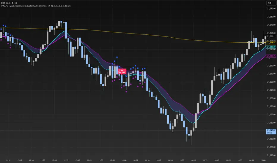
VWAP + EMA Retracement Indicator SwiftEdgeVWAP + EMA Retracement Indicator
Overview
The VWAP + EMA Retracement Indicator is a powerful and visually engaging tool designed to help traders identify high-probability buy and sell opportunities in trending markets. By combining the Volume Weighted Average Price (VWAP) with two Exponential Moving Averages (EMAs) and a unique retracement-based signal logic, this indicator pinpoints moments when the price pulls back to a key zone before resuming its trend. Its modern, AI-inspired visuals and customizable features make it both intuitive and adaptable for traders of all levels.
What It Does
This indicator generates buy and sell signals based on a sophisticated yet straightforward strategy:
Buy Signals: Triggered when the price is above VWAP, has recently retraced to the zone between two EMAs (default 12 and 21 periods), and a strong bullish candle closes above both EMAs.
Sell Signals: Triggered when the price is below VWAP, has retraced to the EMA zone, and a strong bearish candle closes below both EMAs.
Signal Filtering: A customizable cooldown period ensures that only the first signal in a sequence is shown, reducing noise while preserving opportunities for new trends.
Confidence Scores: Each signal includes an AI-inspired confidence score (0-100%), calculated from candle strength and price distance to VWAP, helping traders gauge signal reliability.
The indicator’s visuals enhance decision-making with dynamic gradient lines, a highlighted retracement zone, and clear signal labels, all customizable to suit your preferences.
How It Works
The indicator integrates several components that work together to create a cohesive trading tool:
VWAP: Acts as a dynamic support/resistance level, reflecting the average price weighted by volume. It filters signals to ensure buys occur in uptrends (price above VWAP) and sells in downtrends (price below VWAP).
Dual EMAs: Two EMAs (default 12 and 21 periods) define a retracement zone where the price is likely to consolidate before continuing its trend. Signals are generated only after the price exits this zone with conviction.
Retracement Logic: The indicator looks for price pullbacks to the EMA zone within a user-defined lookback window (default 5 candles), ensuring signals align with trend continuation patterns.
Candle Strength: Signals require strong candles (bullish for buys, bearish for sells) with a minimum body size based on the Average True Range (ATR), filtering out weak or indecisive moves.
Cooldown Mechanism: A unique feature that prevents signal clutter by allowing only the first signal within a user-defined period (default 3 candles), balancing responsiveness with clarity.
Confidence Score: Combines candle body size and price distance to VWAP to assign a score, giving traders an at-a-glance measure of signal strength without needing external analysis.
These components are carefully combined to capture high-probability setups while minimizing false signals, making the indicator suitable for both short-term and swing trading.
How to Use It
Add to Chart: Apply the indicator to a 15-minute chart (recommended) or your preferred timeframe.
Customize Settings:
VWAP Source: Choose the price source (default: hlc3).
EMA Periods: Adjust the fast and slow EMA periods (default: 12 and 21).
Retracement Window: Set how many candles to look back for retracement (default: 5).
ATR Period & Body Size: Define candle strength requirements (default: 14 ATR period, 0.3 multiplier).
Cooldown Period: Control the minimum candles between signals (default: 3; set to 0 to disable).
Candle Requirements: Toggle whether signals require bullish/bearish candles or entire candle above/below EMAs.
Visuals: Enable/disable gradient colors, retracement zone, confidence scores, and choose a color scheme (Neon, Light, or Dark).
Interpret Signals:
Buy: A green "Buy" label with a confidence score appears below the candle when conditions are met.
Sell: A red "Sell" label with a confidence score appears above the candle.
Use the confidence score to prioritize higher-probability signals (e.g., above 80%).
Trade Management: Combine signals with your risk management strategy, such as setting stop-loss below the retracement zone and targeting a 1:2 risk-reward ratio.
Why It’s Unique
The VWAP + EMA Retracement Indicator stands out due to its thoughtful integration of classic indicators with modern enhancements:
Balanced Signal Filtering: The cooldown mechanism ensures clarity without missing key opportunities, unlike many indicators that overwhelm with frequent signals.
AI-Inspired Confidence: The confidence score simplifies decision-making by quantifying signal strength, mimicking advanced analytical tools in an accessible way.
Elegant Visuals: Dynamic gradients, a highlighted retracement zone, and customizable color schemes (Neon, Light, Dark) create a sleek, futuristic interface that’s both functional and visually appealing.
Flexibility: Extensive customization options let traders tailor the indicator to their style, from conservative swing trading to aggressive scalping.
PVSRA Volume Suite with Volume DeltaPVSRA Volume Suite with Volume Delta
🔹 Overview
This indicator is a Volume Suite that enhances PVSRA (Price, Volume, Support, Resistance Analysis) by incorporating Volume Delta and AI-driven predictive alerts. It is designed to help traders analyze volume pressure, market trends, and price movements with color-coded visualizations.
📌 Key Features
PVSRA Volume Color Coding – Highlights vector candles based on extreme volume/spread conditions.
Volume Delta Analysis – Tracks buying/selling pressure using up/down volume data.
AI-Powered Predictive Alerts – Identifies potential trend shifts based on volume and trend context.
Volatility-Adjusted Thresholds – Dynamically adapts volume conditions based on ATR (Average True Range).
Customizable MA & Symbol Overrides – Allows traders to tweak settings for personalized market insights.
Debug & Diagnostic Labels – Shows statistical z-scores, thresholds, and volume dynamics.
How It Works
PVSRA Color Coding – The script classifies candles into four categories based on volume and spread analysis:
🔴 Red Vector → Extreme bearish volume/spread
🟢 Green Vector → Extreme bullish volume/spread
🟣 Violet Vector → Above-average bearish volume
🔵 Blue Vector → Above-average bullish volume
Volume Delta Calculation – Uses lower timeframe volume analysis to estimate up/down volume differentials.
Trend & Predictive Alerts – Combines EMA crossovers with statistical volume analysis to detect potential trend shifts.
Volatility Adaptation – Adjusts volume thresholds based on ATR, making signals more reliable in changing market conditions.
Custom Symbol Override – Fetches PVSRA data from a different instrument, useful for index-based volume analysis.
Customizable Inputs
PVSRA Color Settings – Modify candle color schemes for better visual clarity.
Volume Delta Colors – Customize delta volume body, wick, and border colors.
AI Settings – Tune z-score thresholds, lookback periods, and enable predictive alerts.
Symbol Overrides – Analyze volume from a different market or asset.
Moving Average (MA) Settings – Display a volume-based moving average for trend confirmation.
Important Notes
Works best on intraday timeframes where volume data is reliable.
Lower timeframe volume delta estimates might not be precise for all assets.
No guarantees of accuracy – Use alongside other confluence tools for decision-making.
Credits & Open-Source Notice
This script is based on PVSRA methodologies and integrates Volume Delta analysis. Special thanks to Traders Reality and TradingView for their contributions to volume-based analysis.
MEMEQUANTMEMEQUANT
This script is a comprehensive and specialized tool designed for tracking trends and money flow within meme coins and DEX tokens. By combining various features such as trend lines, Fibonacci levels, and category-based indices, it helps traders make informed decisions in highly volatile markets.
Key Features:
1. Category-Based Indices:
• Tracks the performance of token categories like:
• AI Agent Tokens
• AI Tokens
• Animal Tokens
• Murad Picks
• Each category consists of leader tokens, which are selected based on their higher market cap and trading volume. These tokens act as benchmarks for their respective categories.
• Visualizes category indices in a line chart to identify trends and compare money flow between categories.
2. Fibonacci Correction Zones:
• Highlights key retracement levels (e.g., 60%, 70%, 80%).
• These levels are crucial for identifying potential reversal zones, commonly observed in meme coin trading patterns.
• Fully customizable to match individual trading strategies.
3. Trend Lines:
• Automatically detects major support and resistance levels.
• Separates long-term and short-term trend lines, allowing traders to focus on significant price movements.
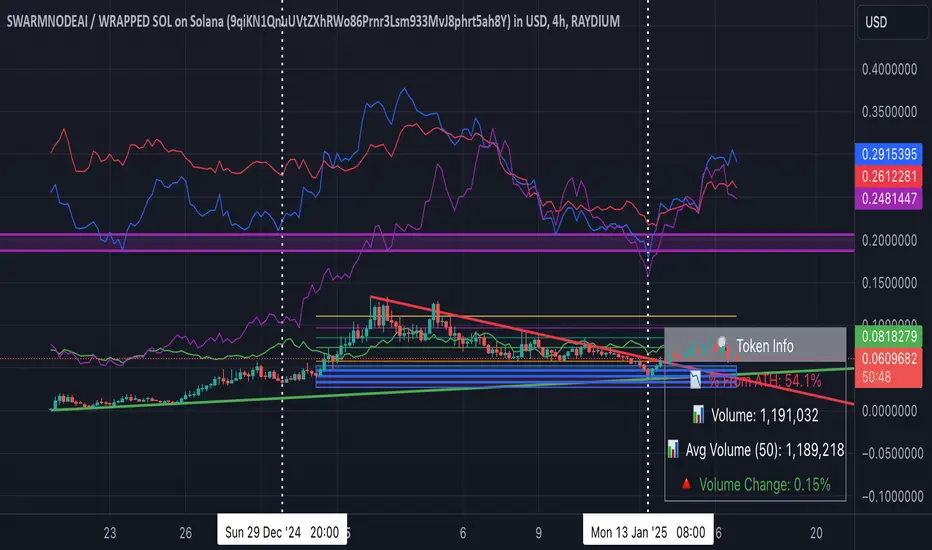
4. Enhanced Info Table:
• Provides real-time insights, including:
• % Distance from All-Time High (ATH)
• Current Trading Volume
• 50-bar Average Volume
• Volume Change Percentage
• Displays information in an easy-to-read table on the chart.
5. Customizable Settings:
• Users can adjust transparency, colors, and ranges for Fibonacci zones, trend lines, and the table.
• Enables or disables individual features (e.g., Fibonacci, trend lines, table) based on preferences.
How It Works:
1. Tracking Money Flow Across Categories:
• The script calculates the market cap to volume ratio for each category of tokens to help identify the dominant trend.
• A higher ratio indicates greater liquidity and stability, while a lower ratio suggests higher volatility or price manipulation.
2. Identifying Retracement Patterns:
• Leverages common retracement behaviors (e.g., 70% correction levels) observed in meme coins to detect potential reversal zones.
• Combines this with trend line analysis for additional confirmation.
3. Leader Tokens as Indicators:
• Each category is represented by its leader tokens, which have historically higher liquidity and market cap. This allows the script to accurately reflect the overall trend in each category.
When to Use:
• Trend Analysis: To identify which category (e.g., AI Tokens or Animal Tokens) is leading the market.
• Reversal Zones: To spot potential support or resistance levels using Fibonacci zones.
• Money Flow: To understand how capital is moving across different token categories in real time.
Who Is This For?
This script is tailored for:
• Traders specializing in meme coins and DEX tokens.
• Those looking for an edge in trend-based trading by analyzing market cap, volume, and retracement levels.
• Anyone aiming to track money flow dynamics between different token categories.
Future Updates:
This is the initial version of the script. Future updates may include:
• Support for additional token categories and DEX data.
• More advanced pattern recognition and alerts for volume and price anomalies.
• Enhanced visualization for historical data trends.
With this tool, traders can combine money flow analysis with the 60-70% retracement strategy, turning it into a powerful assistant for navigating the fast-paced world of meme coins and DEX tokens.
This script is designed to provide meaningful insights and practical utility for traders, adhering to TradingView’s standards for originality, clarity, and user value.
[Pandora] Error Function Treasure Trove - ERF/ERFI/Sigmoids+PRAISE:
At this time, I have to graciously thank the wonderful minds behind the new "Pine Profiler Mode" (PPM). Directly prior to this release, it allowed me to ascertain script performance even more. While I usually write mostly in highly optimized Pine code, PPM visually identified a few bottlenecks that would otherwise be hard to identify. Anyone who contributed to PPMs creation and testing before release... BRAVO!!! I commend all of those who assisted in it's state-of-the-art engineering and inception, well done!
BACKSTORY:
This script is specifically being released in defense of another member, an exceptionally unique PhD. It was brought to my attention that a script-mod-event occurred, regarding the publishing of a measly antiquated error function (ERF) calculation within his script. This sadly resulted in the now former member jumping ship after receiving unmannerly responses amidst his curious inquiries as to why his erf() was modded. To forbid rusty and rudimentary formulations because a mod-on-duty is temporally offended by a non-nefarious release of code, is in MY opinion an injustice to principles of perpetuating open-source code intended to benefit thousands to millions of community members. While Pine is the heart and soul of TV, the mathematical concepts contributed from the minds of members is the inspirational fuel of curiosity that powers it's pertinent reason to exist and evolve.
It is an indisputable fact that most members are not greatly skilled Pine Poets. Many members may be incapable of innovating robust function code in Pine, even if they have one or more PhDs. We ALL come from various disciplines of mathematical comprehension and education. Some mathematicians are not greatly skilled at coding, while some coders are not exceptional at math. So... what am I to do to attempt to resolve this circumstantial challenge??? Those who know me best are aware that I will always side with "the right side of history" in order to accomplish my primary self-defined missions I choose to accept. Serving as an algorithmic advocate, I felt compelled to intercede by compiling numerous error functions into elegant code of very high caliber that any and every TV member may choose to employ, so this ERROR never happens again.
After weeks of contemplation into algorithms I knew little about, I prioritized myself to resolve an unanticipated matter by creating advanced formulas of exquisitely crafted error functions refined to the best of my current abilities. My aversion for unresolved problems motivated me to eviscerate error function insufficiencies with many more rigid formulations beyond what is thought to exist. ERF needed a proper algorithmic exorcism anyways. In my furiosity, I contemplated an array of madMAXimum diplomatic demolition methods, choosing the chain saw massacre technique to slaughter dysfunctionalities I encountered on a battered ERF roadway. This resulted in prolific solutions that should assuredly endure the test of time. Poetically, as you will come to see, I am ripping the lid off of Pandora's box of error functions in this case to correct wrongs into a splendid bundle of rights for members.
INTENTION:
Error function (ERF) enthusiasts... PREPARE FOR GLORY!! The specific purpose of this script is to deprecate classic error functions with the creation of a fierce and formidable army of superior formulations, each having varying attributes of computational complexity with differing absolute error ranges in their results for multiple compute scenarios. This is NOT an indicator... It is intended to allow members to embark on endeavors to advance the profound knowledge base of this growing worldwide community of 60+ million inquisitive minds. For those of you who believe computational mathematics and statistics is near completion at its finest; I am here to inform you, this is ridiculous to ponder. We are no where near statistical excellence that can and will exist eventually. At this time, metaphorically speaking, we are merely scratching microns off of the surface of the skin of a statistical apple Isaac Newton once pondered.
THIS RELEASE:
Following weeks of pondering methodical experiments beyond the ordinary, I am liberating these wild notions of my error function explorations to the entire globe as copyleft code, not just Pine. This Pandora's basket of ERFs is being openly disclosed for the sake of the sanctity of mathematics, empirical science (not the garbage we are told by CONTROLocrats to blindly trust), revolutionary cutting edge engineering, cosmology, physics, information technology, artificial intelligence, and EVERY other mathematical branch of human knowledge being discovered over centuries. I do believe James Glaisher would favor my aims concerning ERF aspirations embracing the "Power of Pine".
The included functions are intended for TV members to use in any way they see fit. This is a gift to ALL members to foster future innovative excellence on this platform. Any attempt to moderate this code without notification of "self-evident clear and just cause" will be considered an irrevocable egregious action. The original foundational PURPOSE of establishing script moderation (I clearly remember) was primarily to maintain active vigilance over a growing community against intentional nefarious actions and/or behaviors in blatant disrespect to other author's works AND also thwart rampant copypasting bandit operations, all while accommodating balanced principles of fairness for an educational community cause via open source publishing that should support future algorithmic inventions well beyond my lifespan.
APPLICATIONS:
The related error functions are used in probability theory, statistics, and numerous and engineering scientific disciplines. Its key characteristics and applications are innumerable in computational realms. Its versatility and significance make it a fundamental tool in arenas of quantitative analysis and scientific research...
Probability Theory - Is widely used in probability theory to calculate probabilities and quantiles of the normal distribution.
Statistics - It's related to the Gaussian integral and plays a crucial role in statistics, especially in hypothesis testing and confidence interval calculations.
Physics - In physics, it arises in the study of diffusion equations, quantum mechanics, and heat conduction problems.
Engineering - Applications exist in engineering disciplines such as signal processing, control theory, and telecommunications.
Error Analysis - It's employed in error analysis and uncertainty quantification.
Numeric Approximations - Due to its lack of a closed-form expression, numerical methods are often employed to approximate erf/erfi().
AI, LLMs, & MACHINE LEARNING:
The error function (ERF) is indispensable to various AI applications, particularly due to its relation to Gaussian distributions and error analysis. It is used in Gaussian processes for regression and classification, probabilistic inference for Bayesian networks, soft margin computation in SVMs, neural networks involving Gaussian activation functions or noise, and clustering algorithms like Gaussian Mixture Models. Improved ERF approximations can enhance precision in these applications, reduce computational complexity, handle outliers and noise better, and improve optimization and convergence, possibly leading to more accurate, efficient, and robust AI systems.
BONUS ALGORITHMS:
While ERFs are versatile, its opposite also exists in the form of inverse error functions (ERFIs). I have also included a modified form of the inverse fisher transform along side MY sigmoid (sigmyod). I am uncertain what sigmyod() may be used for, but it's a culmination of my examinations deep into "sigmoid domains", something I am fascinated by. Whatever implications it may possess, I am unveiling it along with it's cousin functions. For curious minds, this quality of composition seen here is ideally what underlies what I would term "Pandora functionality" that empowers my Pandora indication. I go through hordes of formulations, testing, and inspection to find what appears to be the most beneficial logical/mathematical equation to apply...
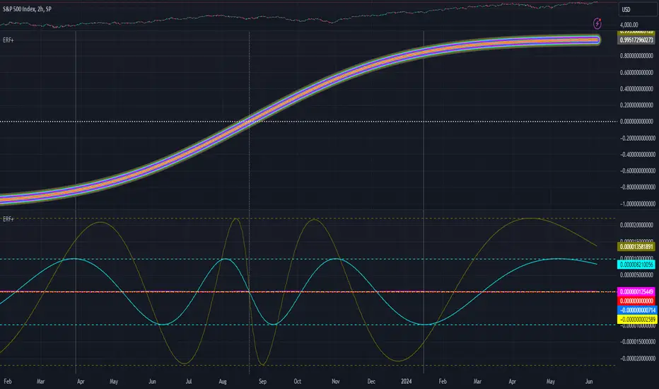
SCRIPT OPERATION:
To showcase the characteristics and performance of my ERF/ERFI formulations, I devised a multi-modal script. By using bar_index , I generated a broad sequence of numeric values to input into the first ERF/ERFI parameter. These sequences allow you to inspect the contours of the error function's outputs for both ERF and ERFI. When combined with compute-intensive precision functions (CIPFs), the polynomial function output values can be subtracted from my CIPFs to obtain results of absolute error, displaying the accuracy of the many polynomial estimation functions I tuned in testing for Pine's float environment.
A host of numeric input settings are wildly adjustable to inspect values/curvatures across the range of numeric input sequences. Very large numbers, such as Divisor:100,000,100/Offset:200,000,000 for ERF modes or... Divisor:100,000,100/Offset:100,000,000 for ERFI modes, will display miniscule output values calculated from input values in close proximity to 0.0 for the various estimates, similar to a microscope. ERFI approximations very near in proximity to +/-1.0 will always yield large deviations of absolute error. Dragging/zooming your chart or using the Offset input will aid with visually clipping off those ERFI extremes where float precision functions cannot suffice.
NOTICE:
perf() and perfi() are intended for precision computation (as good as it basically gets) in a float environment. However, they are CPU intensive (especially perfi). I wouldn't recommend these being used in ANY Pine script unless it's an "absolute necessity" to do so to accomplish your goal. I only built them to obtain "absolute error curvatures" of the error functions for the polynomial approximations. These are visible in the accuracy modes in the indicator Settings.
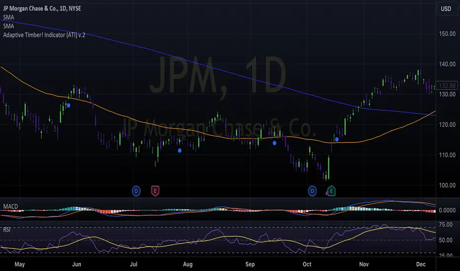
Adaptive Timber! Indicator (ATI)The Adaptive Timber! Indicator (ATI) is a powerful tool designed to identify potential overbought conditions and generate reversal signals in financial markets. It combines multiple technical indicators and market conditions to provide a comprehensive assessment of the likelihood of a price reversal.
How it works:
The ATI uses a combination of the Relative Strength Index (RSI), Moving Average Convergence Divergence (MACD), momentum, and volume to detect overbought conditions and potential reversals. The indicator adapts to the current timeframe, adjusting its parameters accordingly to provide more accurate signals.
Key components:
RSI: The ATI uses the RSI to determine overbought conditions. When the RSI exceeds a specified reversal threshold, it indicates a potential overbought state.
MACD: The indicator monitors the MACD line and signal line to identify moments when they are close to crossing, suggesting a potential trend reversal.
Momentum: The ATI checks if the momentum is increasing, providing confirmation of a potential reversal.
Volume: It analyzes volume to confirm the strength of the reversal signal. A decrease in volume along with overbought conditions adds confidence to the reversal indication.
Timeframe Adaptability: The indicator automatically adjusts its parameters based on the current timeframe, ensuring optimal performance across different time horizons.
How to use:
When the ATI identifies a potential reversal, it displays a colored triangle above the price bars. The color of the triangle represents the strength of the reversal signal: red for a strong signal, orange for a moderate signal, and yellow for a weak signal. Additionally, the indicator plots purple triangles below the price bars as an early warning signal for potential trend reversals.
Traders can use these visual cues along with other technical analysis techniques and risk management strategies to make informed trading decisions. The ATI can be particularly useful for identifying potential short-selling opportunities or for determining exit points in existing long positions.
Creators:
The Adaptive Timber! Indicator (ATI) is the result of a collaborative effort led by Claude , an AI assistant with expertise in financial analysis and programming. The development of the ATI was made possible through the valuable contributions and insights from GPT4 , an advanced language model, Clay , a skilled trader, and Pi AI , Clay's trading assistant.
Claude played a crucial role in designing and implementing the indicator's algorithm, ensuring its robustness and adaptability across different timeframes. GPT4 provided guidance and suggestions for refining the indicator's logic and optimizing its performance. Clay and Pi AI offered their trading expertise and real-world experience to help shape the indicator's functionality and usability.
We would like to express our gratitude to all the members of our trading team for their dedication and hard work in bringing the Adaptive Timber! Indicator to life. We wish all traders the best of luck in their trading endeavors and hope that the ATI will be a valuable addition to their technical analysis toolkit, empowering them to make more informed and profitable trading decisions.
My exponential moving averages - Suri's EMAs
It's not an indication of anything here, it's just part of my operating in a simple and summarized way, I hope it helps someone.
Suri's EMA's indicator is nothing more than a set of exponential moving averages (EMA). They are 12, 26, 50 and 200.
Attention to the use of the indicator, it is just an INDICATOR, it should not be taken as the main point of your entry, but to guide you in your entries in favor of the trend, whether intra-day or swing.
Created for clear, monochrome screens. Make your adjustments.
Color condition, candles turn green when their close is above EMA 12 and 26.
Color condition, candles turn red when their close is below EMA 12 and 26.
Condition for colors, MME12,26,50 and 200 will turn green with price working above it.
Condition for colors, MME12, 26, 50 and 200 will turn red with price working below it.
Indication for use in time-frames = 5m, 15m, 60m, 240m. (higher hit rates)
How to use the indicator, MME 12 and 26, are the most important and led you to more entries, but we should not only consider them, we have to analyze the whole context to then make a decision.
Indicator was nicknamed by me by "Pullback Pick", it works in a simple way:
In an uptrend or downtrend, the price usually tends to return in the averages or the averages go up to the price, that being said, it is easy to observe that where the price returns would be a pullback from the last movement, so when returning to the averages, the candle that shows strength in favor of this trend, in the EMA's region, becomes a possible entry, with its stop below or above this "pullback" formed, because the stop goes there, because usually when the price returns on the EMAs they tend to to hold and replay the price in favor of the trend.
My observations:
I like to enter when the price returns to the averages smoothly, without much movement, when it touches the average 12 or 26 it is an entry, but an entry without confirmation, the gain is greater, but the chance of being stopped is higher, I like it when the price is close to the 12 and 26 averages and leaves a small candle or doji on this pullback, my entry goes to the breakout of this candle and the stop behind the candle.
THERE IS NO MIRACLE, THERE IS NO 100% HIT RATE, SO USE STOP.
Aaaaaaaaaa I was forgetting.... and the target???
As it is a trend following setup, it is cool to leave a trailing stop or update the stop as new bottoms or tops are formed.
Targeting in 1v1 is good, setup pays a lot!
Targeting in 2x1 is too good, setup pays well!
Making a target in 3x1 is more than good, setup pays sometimes, then from now on, it depends on where you are entering this "PULLBACK", if it is in the first wave, in the second, if you are going to lateralize, the market is SOVEREIGN, put in the pocket that is no longer on the market, oh it's yours!
That's it, doubts, send it there, suggestion, opinion, whatever you want.
Added a symbol at the crossing of the 12 and 26 moving averages.
I am so sorry, but i dont speak english, use google translate.
Português.
Não se trata de indicação de nada aqui, é apenas parte do meu operacional de maneira simples e resumida, espero que ajude alguém.
Indicador Suri's EMA's, nada mais é do que um conjunto de médias móveis exponenciais(MME). São elas 12, 26, 50 e 200.
Atenção para o uso do indicador, ele é apenas um INDICADOR, não deve ser tomado como o ponto principal de sua entrada, mas sim de te balizar nas suas entradas a favor da tendência, seja ela intra-day ou swing.
Criado para telas claras e monocromáticas. Façam seus ajustes.
Condição para as cores, candles ficam verdes quando o fechamento dele é acima das MME 12 e 26.
Condição para as cores, candles ficam vermelhos quando o fechamento dele é abaixo das MME 12 e 26.
Condição para as cores, MME12,26,50 e 200 ficará verde com preço trabalhando acima dela.
Condição para as cores, MME12, 26, 50 e 200 ficará vermelho com preço trabalhando abaixo dela.
Indicação para uso nos time-frame = 5m, 15m, 60m, 240m.(taxas de acerto maior)
Como utilizar o indicador, MME 12 e 26, são as mais importantes e te levaram a mais entradas, porém não devemos levar apenas elas em consideração, temos que analisar todo o contexto para então tomar decisão.
Indicador foi apelidado por mim por " Pega Pullback", ele funciona de uma maneira simples:
Em tendência de alta ou de baixa, o preço geralmente tende a retornar nas médias ou as médias irem até o preço, dito isso é fácil de se observar que onde o preço retorna seria um pullback do último movimento, portanto ao retornar nas médias, o candle que mostra força a favor dessa tendência, na região das EMA's, se torna uma possível entrada, com o seu stop abaixo ou acima desse "pullback" formado, porque o stop vai nesse local, porque geralmente quando o preço retorna nas EMAs elas tendem a segurar e voltar a jogar o preço a favor da tendência.
Minhas observações:
Eu gosto de entrar quando o preço retorna nas médias de maneira suave, sem muito movimento, quando toca na média 12 ou 26 é uma entrada, porém uma entrada sem confirmação, o ganho é maior, porém a chance de ser stopado é mais alta, eu gosto quando o preço fica perto das médias 12 e 26 e deixa um candle pequeno ou doji nesse pullback, minha entrada vai no rompimento desse candle e o stop atrás do candle.
Não existe MILAGRE, NÃO EXISTE TAXA DE ACERTO DE 100%, POR ISSO USE STOP.
Aaaaaaaaaa ia me esquecendo.... e o alvo???
Por ser um setup seguidor de tendência, o legal é deixar um trailing stop ou ir atualizando o stop conforme novos fundos ou topos são formados.
Realizar alvo no 1x1 é bom, setup paga muito!
Realizar alvo no 2x1 é bom de mais, setup paga bem!
Realizar alvo no 3x1 é mais do que bom, setup paga as vezes, ai daqui pra frente, depende de onde você está entrando nesse "PULLBACK", se é na primeira onda, na segunda, se vai lateralizar, o mercado é SOBERANO, põe no bolso que não é mais do mercado, ai é teu!
É isso, dúvidas, manda ai, sugestão, opinião, o que quiser.
Adicionado um símbolo no cruzamento das médias móveis 12 e 26.

stelaraX - Williams %RstelaraX – Williams %R
stelaraX – Williams %R is a momentum oscillator designed to identify overbought and oversold market conditions. It measures the position of the current close relative to the highest high and lowest low over a defined lookback period and reacts quickly to changes in market momentum.
This indicator is part of the stelaraX ecosystem, focused on clean technical analysis and AI-supported chart evaluation
stelarax.com
Core logic
Williams %R is calculated over a user-defined period and oscillates between 0 and -100.
Key characteristics include:
* values near 0 indicate overbought conditions
* values near -100 indicate oversold conditions
* the -50 level acts as a momentum midpoint
When Williams %R moves above the overbought threshold, bullish momentum may be stretched. When it moves below the oversold threshold, bearish momentum may be stretched.
Visualization
The script plots:
* the Williams %R line in a separate indicator pane
* a configurable overbought level
* a configurable oversold level
* a midline at -50 for directional context
The area between the overbought and oversold levels is visually highlighted, making extreme momentum conditions easy to identify.
Use case
This indicator is intended for:
* identifying overbought and oversold market conditions
* spotting potential momentum reversals
* confirming short-term trend exhaustion
* divergence analysis between price and momentum
* timing entries and exits in ranging or trending markets
For traders who want to combine classical oscillators with modern AI-driven chart analysis, additional tools and insights are available at stelarax.com
Disclaimer
This indicator is provided for educational and technical analysis purposes only and does not constitute financial advice or trading recommendations. All trading decisions and risk management remain the responsibility of the user.

stelaraX - MomentumstelaraX – Momentum
stelaraX – Momentum is a simple yet effective indicator designed to measure the speed and direction of price movement. It shows whether price is accelerating or decelerating and helps identify shifts in market strength at an early stage.
This indicator is part of the stelaraX ecosystem, focused on clean technical analysis and AI-supported chart evaluation
stelarax.com
Core logic
The Momentum indicator calculates the difference between the current price and the price from a user-defined number of periods ago.
Key characteristics include:
* positive values indicate upward momentum
* negative values indicate downward momentum
* the zero line acts as a directional threshold
When momentum crosses above zero, bullish pressure is increasing. When momentum crosses below zero, bearish pressure is increasing.
Visualization
The script plots a histogram in a separate indicator pane:
* green bars when momentum is positive
* red bars when momentum is negative
* a clearly visible zero baseline for direction reference
The histogram format makes changes in momentum strength immediately visible.
Use case
This indicator is intended for:
* measuring price acceleration and deceleration
* confirming trend strength
* identifying early momentum shifts
* filtering entries in trend-following strategies
* divergence analysis between price and momentum
For traders who want to combine classical momentum tools with modern AI-driven chart analysis, additional tools and insights are available at stelarax.com
Disclaimer
This indicator is provided for educational and technical analysis purposes only and does not constitute financial advice or trading recommendations. All trading decisions and risk management remain the responsibility of the user.

stelaraX - MFIstelaraX – MFI
stelaraX – MFI is a volume-weighted momentum oscillator that combines price movement and trading volume to measure buying and selling pressure. Unlike pure price-based oscillators, the Money Flow Index incorporates volume, making it especially useful for identifying strength behind price moves.
This indicator is part of the stelaraX ecosystem, focused on clean technical analysis and AI-supported chart evaluation
stelarax.com
Core logic
The Money Flow Index is calculated using the typical price (HLC3) and volume over a user-defined lookback period.
The calculation distinguishes between positive and negative money flow and converts the result into an oscillator ranging from 0 to 100.
Key components include:
* MFI value between 0 and 100
* overbought threshold to identify excessive buying pressure
* oversold threshold to identify excessive selling pressure
High MFI values indicate strong inflows of capital, while low values indicate capital outflows.
Visualization
The script plots:
* the MFI line in a separate indicator pane
* a configurable overbought level
* a configurable oversold level
The area between overbought and oversold levels is visually highlighted, allowing quick recognition of extreme money flow conditions.
Use case
This indicator is intended for:
* identifying overbought and oversold conditions with volume confirmation
* spotting potential reversals driven by volume imbalance
* confirming price trends with underlying money flow
* divergence analysis between price and volume-based momentum
* filtering trades based on participation strength
For traders who want to combine price action with volume-aware, AI-driven chart analysis, additional tools and insights are available at stelarax.com
Disclaimer
This indicator is provided for educational and technical analysis purposes only and does not constitute financial advice or trading recommendations. All trading decisions and risk management remain the responsibility of the user.

stelaraX - Heikin AshistelaraX – Heikin Ashi
stelaraX – Heikin Ashi is a price-smoothing indicator that transforms standard candlestick data into Heikin Ashi candles. By averaging price values, it reduces market noise and makes trend direction and momentum easier to read directly on the chart.
This indicator is part of the stelaraX ecosystem, focused on clean technical analysis and AI-supported chart evaluation
stelarax.com
Core logic
Heikin Ashi candles are calculated using averaged price values instead of raw open and close data.
Each candle is derived from:
* averaged open based on the previous Heikin Ashi candle
* averaged close based on the current candle’s OHLC values
* high and low adjusted to reflect the full price range
This calculation smooths price action and filters out short-term volatility, allowing trends to appear more consistent and structured.
Visualization
The script plots custom Heikin Ashi candles directly on the price chart:
* bullish candles displayed in a configurable bullish color
* bearish candles displayed in a configurable bearish color
* candle bodies, wicks, and borders are fully color-aligned
The result is a clean and uniform visual representation of trend strength and direction.
Use case
This indicator is intended for:
* identifying and following market trends
* reducing noise in choppy market conditions
* improving trend clarity for discretionary trading
* confirming trend direction in combination with other indicators
* simplifying price structure for higher-level analysis
For traders who want to combine smoothed price action with modern AI-driven chart analysis, additional tools and insights are available at stelarax.com
Disclaimer
This indicator is provided for educational and technical analysis purposes only and does not constitute financial advice or trading recommendations. All trading decisions and risk management remain the responsibility of the user.

stelaraX - EnvelopestelaraX – Envelope
stelaraX – Envelope is a price channel indicator based on a moving average with fixed percentage bands above and below the average. It is designed to visualize dynamic support and resistance zones and highlight potential overextended market conditions.
This indicator is part of the stelaraX ecosystem, focused on clean technical analysis and AI-supported chart evaluation
stelarax.com
Core logic
The indicator calculates a central moving average using either:
* exponential moving average (EMA)
* simple moving average (SMA)
Upper and lower envelope bands are then derived by applying a fixed percentage offset to the moving average.
The distance between price and the envelope bands reflects relative market extension. Price near or beyond the outer bands may indicate overbought or oversold conditions depending on context and trend direction.
Visualization
The script plots:
* the central moving average
* an upper envelope band
* a lower envelope band
The area between the upper and lower bands is softly filled to improve visual clarity and make price deviations easy to identify at a glance.
Use case
This indicator is intended for:
* identifying dynamic support and resistance zones
* detecting overextended price conditions
* mean reversion and pullback analysis
* trend-following confirmation when combined with other indicators
* channel-based trade planning
For traders who want to combine classical price channels with modern AI-driven chart analysis, additional tools and insights are available at stelarax.com
Disclaimer
This indicator is provided for educational and technical analysis purposes only and does not constitute financial advice or trading recommendations. All trading decisions and risk management remain the responsibility of the user.

stelaraX - VWAPstelaraX – VWAP
stelaraX – VWAP is a volume-weighted price indicator designed to show the average traded price of an asset throughout the trading session. By incorporating volume into the calculation, it provides a more realistic view of fair value compared to simple price averages.
This indicator is part of the stelaraX ecosystem for clean technical analysis and AI-supported chart evaluation.
stelarax.com
Core logic
The indicator calculates the Volume Weighted Average Price using the typical price (HLC3) and traded volume.
VWAP represents the average price at which the market has traded, weighted by volume, and is commonly used to assess whether price is trading at a premium or discount relative to fair value.
Optional deviation bands are calculated using the volume-weighted standard deviation around the VWAP. Two configurable band levels allow traders to measure statistical price extremes.
Visualization
The script plots:
* the VWAP line directly on the price chart
* optional upper and lower deviation bands
* two configurable deviation multipliers
The VWAP line serves as the central reference, while the bands highlight potential overextension zones above and below the average traded price.
Use case
This indicator is intended for:
* identifying fair value and premium or discount pricing
* intraday trend bias and mean reversion analysis
* dynamic support and resistance assessment
* trade filtering and execution alignment
* combining volume context with price structure
For traders who want to integrate volume-based analysis with modern AI-driven chart evaluation, additional tools and insights are available at stelarax.com
Disclaimer
This indicator is provided for educational and technical analysis purposes only and does not constitute financial advice or trading recommendations. All trading decisions and risk management remain the responsibility of the user.

stelaraX - SupertrendstelaraX – Supertrend
stelaraX – Supertrend is a trend-following indicator based on the Average True Range (ATR). It dynamically adapts to market volatility and provides clear visual guidance for identifying bullish and bearish trend phases directly on the chart.
This indicator is part of the stelaraX ecosystem, focused on clean technical analysis and AI-supported chart evaluation.
stelarax.com
Core logic
The Supertrend is calculated using two user-defined parameters:
* ATR period
* volatility factor
The indicator uses ATR-based price bands to determine trend direction:
* bullish trend when price holds above the Supertrend level
* bearish trend when price holds below the Supertrend level
When price crosses the Supertrend line, the trend direction flips accordingly. The ATR factor controls the sensitivity of trend changes, with higher values producing fewer but stronger signals.
Visualization
The script plots a single Supertrend line directly on the price chart:
* green color during bullish trends
* red color during bearish trends
* broken line style to clearly show trend transitions
The minimalist design ensures that trend direction is immediately visible without cluttering the chart.
Use case
This indicator is intended for:
* identifying and following market trends
* defining dynamic trailing stop levels
* filtering trades in the direction of the dominant trend
* trend confirmation in combination with other indicators
For traders looking to combine classical trend tools with modern AI-driven chart analysis, additional tools and insights are available at stelarax.com
Disclaimer
This indicator is provided for educational and technical analysis purposes only and does not constitute financial advice or trading recommendations. All trading decisions and risk management remain the responsibility of the user.

stelaraX - StochasticstelaraX – Stochastic
stelaraX – Stochastic is a momentum oscillator designed to compare the current closing price to the recent price range over a defined period. It helps identify overbought and oversold conditions and provides early signals for potential momentum shifts.
This indicator is part of the stelaraX ecosystem, focused on clean technical analysis and AI-supported chart evaluation.
stelarax.com
Core logic
The Stochastic oscillator is calculated using three configurable parameters:
* %K lookback period
* %K smoothing
* %D smoothing
The indicator consists of:
* the %K line, representing raw momentum
* the %D line, a smoothed moving average of %K
Momentum is considered bullish when %K is above %D and bearish when %K is below %D. Crossovers between %K and %D can indicate potential trend shifts.
Visualization
The script plots:
* the %K line
* the %D line
* a configurable overbought level
* a configurable oversold level
The area between the overbought and oversold levels is visually highlighted, allowing quick identification of extreme momentum conditions.
Use case
This indicator is intended for:
* identifying overbought and oversold market conditions
* spotting early momentum reversals
* confirming trend continuation or exhaustion
* divergence analysis between price and momentum
For traders who want to combine classical oscillators with modern AI-driven chart analysis, additional tools and insights are available at stelarax.com
Disclaimer
This indicator is provided for educational and technical analysis purposes only and does not constitute financial advice or trading recommendations. All trading decisions and risk management remain the responsibility of the user.

stelaraX - RSIstelaraX – RSI
stelaraX – RSI is a momentum oscillator designed to measure the speed and magnitude of recent price changes. It helps identify overbought and oversold market conditions while providing a clear view of momentum shifts and potential reversals.
This indicator is part of the stelaraX ecosystem, focused on clean technical analysis and AI-supported chart evaluation.
stelarax.com
Core logic
The Relative Strength Index is calculated using a user-defined lookback period and compares average gains to average losses over that period.
Key elements include:
* RSI value oscillating between 0 and 100
* overbought level to identify stretched bullish conditions
* oversold level to identify stretched bearish conditions
* a central 50 level to distinguish bullish and bearish momentum regimes
When RSI is above 50, momentum is considered bullish. When RSI is below 50, momentum is considered bearish.
Visualization
The script plots:
* the RSI line
* a configurable overbought level
* a configurable oversold level
* a neutral midline at 50
The area between overbought and oversold levels is visually highlighted, making momentum zones easy to interpret at a glance.
Use case
This indicator is intended for:
* identifying overbought and oversold conditions
* spotting momentum shifts and potential reversals
* confirming trend strength and continuation
* divergence analysis between price and momentum
For traders looking to combine classical momentum tools with modern AI-driven chart analysis, additional tools and insights are available at stelarax.com
Disclaimer
This indicator is provided for educational and technical analysis purposes only and does not constitute financial advice or trading recommendations. All trading decisions and risk management remain the responsibility of the user.

stelaraX - MACDstelaraX – MACD
stelaraX – MACD is a classic momentum and trend-following indicator based on the relationship between two exponential moving averages. It is designed to visualize trend direction, momentum strength, and potential reversal points in a clear and uncluttered way.
This indicator is part of the stelaraX ecosystem, focused on clean technical analysis and AI-supported chart evaluation.
stelarax.com
Core logic
The MACD is calculated using three user-defined parameters:
* fast moving average period
* slow moving average period
* signal line smoothing period
The indicator consists of:
* the MACD line, calculated as the difference between the fast and slow EMA
* the signal line, which is an EMA of the MACD line
* the histogram, representing the difference between MACD and signal line
Momentum increases when the histogram expands and decreases when it contracts. Crossovers between the MACD line and the signal line highlight potential trend shifts.
Visualization
The script plots:
* the MACD line
* the signal line
* a color-coded histogram
Histogram bars adapt their color dynamically:
* green tones for positive momentum
* red tones for negative momentum
* brighter colors when momentum is increasing
* softer colors when momentum is weakening
A zero baseline is plotted to clearly separate bullish and bearish momentum phases.
Use case
This indicator is intended for:
* momentum and trend analysis
* identifying trend continuation and exhaustion
* confirming price action and breakout signals
* divergence observation between price and momentum
For traders looking to combine classical indicators with modern AI-driven chart analysis, additional tools are available at stelarax.com
Disclaimer
This indicator is provided for educational and technical analysis purposes only and does not constitute financial advice or trading recommendations. All trading decisions and risk management remain the responsibility of the user.

stelaraX - Keltner ChannelstelaraX – Keltner Channel
stelaraX – Keltner Channel is a volatility-based price channel indicator that combines an exponential moving average with the Average True Range to define dynamic upper and lower boundaries around price. The indicator is designed to highlight trend direction, volatility expansion, and potential breakout or mean reversion zones.
For advanced AI-based chart analysis and automated volatility interpretation, visit stelarax.com
Core logic
The indicator calculates the Keltner Channel using three components:
* an exponential moving average as the central basis line
* an upper band defined as EMA plus a multiple of ATR
* a lower band defined as EMA minus a multiple of ATR
Both the EMA period and ATR period are user-configurable, as well as the ATR multiplier, allowing precise control over channel width and sensitivity.
Visualization
The script plots:
* the EMA basis line
* the upper Keltner Channel band
* the lower Keltner Channel band
The area between the upper and lower bands can be filled with a semi-transparent color to clearly visualize the active volatility range. All colors are fully customizable for clean chart integration.
Use case
This indicator is intended for:
* trend-following and channel-based strategies
* identifying volatility expansion and contraction
* breakout and pullback analysis
* dynamic support and resistance evaluation
* combining volatility with trend direction
For a fully automated AI-driven chart analysis solution, additional tools and insights are available at stelarax.com
Disclaimer
This indicator is provided for educational and technical analysis purposes only and does not constitute financial advice or trading recommendations. All trading decisions and risk management remain the responsibility of the user.

stelaraX - Ichimoku CloudstelaraX – Ichimoku Cloud
stelaraX – Ichimoku Cloud is a complete trend and market structure indicator based on the traditional Ichimoku Kinko Hyo system. The indicator visualizes trend direction, momentum, and support and resistance zones using a single integrated framework.
For advanced AI-based chart analysis and automated multi-indicator interpretation, visit stelarax.com
Core logic
The indicator calculates all main Ichimoku components using configurable periods:
* Tenkan-Sen is calculated as the midpoint of the highest high and lowest low over a short period
* Kijun-Sen is calculated as the midpoint over a medium period
* Senkou Span A is the average of Tenkan-Sen and Kijun-Sen and is projected forward
* Senkou Span B is the midpoint over a longer period and is projected forward
* Chikou Span represents current price shifted back by the displacement value
This structure provides a complete view of trend, momentum, and equilibrium.
Visualization
The script plots all Ichimoku elements directly on the chart:
* Tenkan-Sen and Kijun-Sen lines
* Chikou Span plotted backward
* Senkou Span A and Senkou Span B projected forward
* filled cloud area between Senkou spans
The cloud color dynamically reflects bullish or bearish conditions depending on the relationship between Senkou Span A and Senkou Span B.
Use case
This indicator is intended for:
* identifying overall trend direction and strength
* spotting dynamic support and resistance zones
* evaluating momentum and trend continuation
* filtering trades using cloud bias
* multi-timeframe trend alignment
For a fully automated AI-driven chart analysis solution, additional tools and insights are available at stelarax.com
Disclaimer
This indicator is provided for educational and technical analysis purposes only and does not constitute financial advice or trading recommendations. All trading decisions and risk management remain the responsibility of the user.

stelaraX - ATRstelaraX – ATR
stelaraX – ATR is a volatility indicator based on the Average True Range (ATR). It measures the average price movement over a defined period and provides a clear view of current market volatility independent of price direction.
For advanced AI-based chart analysis and automated volatility evaluation, visit stelarax.com
Core logic
The indicator calculates the Average True Range using a user-defined period.
ATR is derived from the true range, which considers:
* current high minus current low
* absolute difference between current high and previous close
* absolute difference between current low and previous close
The ATR value reflects the average volatility over the selected lookback window.
Visualization
The script plots a single ATR line in a separate indicator pane:
* smooth volatility line
* configurable period length
* customizable line color
* clean and minimal visual design
The indicator does not generate signals and is intended purely for volatility assessment.
Use case
This indicator is intended for:
* measuring market volatility
* defining dynamic stop loss and take profit distances
* position sizing and risk management
* identifying volatility expansion or contraction
* filtering trades based on market conditions
For a fully automated AI-driven chart analysis solution, additional tools and insights are available at stelarax.com
Disclaimer
This indicator is provided for educational and technical analysis purposes only and does not constitute financial advice or trading recommendations. All trading decisions and risk management remain the responsibility of the user.
