Signal Algo - Elephant EdgeDescription
Signal Algo - Advance Elephant Edge is a rule-based, intraday detection system that combines candle-pattern logic with session-driven support and resistance zones. creating a clean confluence-based signal that removes noise.
This tool is designed for traders who prefer structured rules over subjective drawing, and want clear, event-driven alerts without unrealistic promises or over-optimized behavior.
What This Script Does (Short & Simple)
1. Hammer-Type Candle Detection
The script looks for long-wick hammer or inverted hammer candles using your wick-ratio setting. It also checks candle size, body size, and doji conditions so that only clean and meaningful rejection candles are highlighted.
2. Session-Based Percentile Support & Resistance
The indicator calculates percentile levels from previous sessions and plots up to four upper and lower S/R lines around the daily open. These levels act as dynamic zones where price often reacts.
3. Optional Strike-Price Zones
For symbols that move around round numbers or strike intervals, the script can draw strike-based S/R lines (like 50 or 100 points) You can choose solid or dotted lines and select how many zones to show.
4.Higher-Timeframe Trend Background
A light green or red background shows the overall trend direction. Green = bullish bias, Red = bearish bias.
🔶 USAGE & EXAMPLES Elephant Support & Resistance
Elephant Support & Resistance creates intraday support and resistance levels using percentile data from previous sessions. Instead of drawing lines manually, calculates how far price usually moves above and below previous sessions. and then plots those levels automatically.
Each percentile pair (Level 1–4) gives one upper line and one lower line. These lines represent price zones where the market has reacted many times in the past. When price reaches these levels, it often pauses, reverses, or shows rejection candles.
🔶USAGE & EXAMPLES Strike Price Support & Resistance
Strike Price Zones are plotted because most markets naturally react around fixed strike levels. Every index, stock, or international market has its own commonly traded strike prices. These levels attract large traders and institutions, who often build positions around them.
When price moves toward one of these strike levels, big players frequently defend or reject that zone. As a result, price may pause, reverse, or show strong reactions at or near these strikes.
Because of this behavior, Strike Price Zones work as practical intraday support and resistance levels. They help traders see where important reactions can occur, where momentum may slow down, and where potential reversals may form.
These zones are not buy/sell signals by themselves, but they provide a simple, objective roadmap of key levels that the market respects during the session.
🔷 FEATURES
1. Hammer-Based Rejection Signals
2. Candle Size Filtering
3. Elephant Percentile Support & Resistance
4. Strike Price Support & Resistance Zones
5. Combined Confluence Logic
6. Higher-Timeframe Trend Background
7. Clean Visual Layout
8. Yellow Highlight Candle
9. Intraday Session Handling
10. Built-In Alerts
11. Fully Customizable Inputs
12. Lightweight & Rule-Driven Design
🔴 RISK DISCLAIMER
Trading is risky & most day traders lose money. All content, tools, scripts, articles, & education provided by Signal Algo are purely for informational & educational purposes only. Past performance does not guarantee future results.
Cerca negli script per "algo"

Sigma-X Algo (Oscillator) Final + DivSigma-X Algo - Divergence & Momentum**
**简介 / Short Description:**
The companion oscillator for the Sigma-X system. Features absolute momentum (TRIMA), structural trend filtering, and automatic divergence detection.
Sigma-X 系统的配套副图指标。包含绝对动能算法、趋势结构过滤以及自动背离检测功能。
**详细描述 / Description:**
---
### ** 中文说明**
这是 **Sigma-X Algo** 系统的专用副图震荡指标,用于辅助主图进行动能确认和背离识别。
#### **核心功能**
1. **动能柱 (Momentum Histogram):**
* 基于价格与 TRIMA 均线的偏离度绘制。
* **实心柱:** 动能增强。
* **空心/浅色柱:** 动能衰竭(这是进场的重要参考)。
2. **👀 自动背离检测 (Auto Divergence):**
* 自动识别价格与动能之间的 **底背离 (Bullish)** 和 **顶背离 (Bearish)**。
* **绿线:** 底背离,提示潜在上涨。
* **红线:** 顶背离,提示潜在下跌。
3. **🦅 鹰眼预警 (Warning Zones):**
* 当动能突破 **1.8σ** 警戒线时,背景会变色,提示即将进入变盘区。
#### **如何配合主图使用**
当主图出现 **S+ 信号** 时,观察副图:
* 如果副图同时出现 **绿线 (底背离)**,胜率极高。
* 如果副图动能柱颜色变浅 (衰竭),确认反转即将发生。
---
### ** English Description**
This is the companion oscillator for the **Sigma-X Algo** system, designed to confirm momentum and identify divergences.
#### **Key Features**
1. **Momentum Histogram:**
* Calculated based on the deviation between Price and TRIMA.
* **Solid Colors:** Momentum is increasing.
* **Pale Colors:** Momentum is exhausting (A key trigger for entry).
2. **👀 Auto Divergence Detection:**
* Automatically plots **Regular Bullish (Green Line)** and **Regular Bearish (Red Line)** divergences between Price and Oscillator.
3. **🦅 Warning Zones:**
* Background changes color when momentum breaches the **1.8σ** warning threshold, signaling potential volatility.
#### **How to Use with Main Chart**
When a **S+ Signal** appears on the Main Chart:
* Look for a **Green Line (Bullish Divergence)** on this oscillator for high-probability confirmation.
* Wait for the histogram bars to fade (exhaustion) before pulling the trigger.

NAS Oracle AlgoThe NAS Oracle Algo is a powerful and versatile daily trading indicator designed to provide clear, automated support and resistance levels for both long and short trading strategies. By calculating a dynamic range based on the previous day's price action, it projects key entry points, stop-losses, and up to six profit targets onto your chart, giving you a complete roadmap for the trading day.
Key Features:
Dual-Sided Strategy: Generates independent levels for BUY and SELL setups, making it effective for both directional and range-bound markets.
Customizable Reference Point: Choose between using the current day's "Open" or the previous day's "Pre Close" as the base for all calculations.
Comprehensive Levels:
Entry Level: The price level to execute a trade.
Stop Loss: A predefined level to limit potential losses.
Profit Targets (1-6): Six incremental take-profit levels, allowing for partial profit-taking strategies.
Multiple Display Options:
Visual Levels & Labels: Clean horizontal lines and text labels are drawn directly on the chart for easy price reference.
Information Table: A highly customizable data table that summarizes all key levels, which can be positioned at the Top or Bottom of the chart and resized.
Flexible Configuration: Toggle the visibility of levels and choose to show either 3 or 6 profit targets to suit your trading style and avoid chart clutter.
How to Use:
Add the Indicator: Apply the "NAS Oracle Algo" to your chart. It works best on daily and intraday timeframes.
Configure Settings: In the indicator's settings, choose your preferred Option (Open/Pre Close), toggle levels and the table on/off, and adjust their position and size.
Interpret the Signals:
BUY Setup: When the price moves above the green "Buy Above" level, consider a long entry.
Stop Loss: Place your stop loss at the BUY_SL level.
Take Profit: Scale out of your position at the six progressively higher target levels (T1 to T6).
SELL Setup: When the price moves below the red "Sell Below" level, consider a short entry.
Stop Loss: Place your stop loss at the SELL_SL level.

Rider Algo 5 & 6 Strategies - RSI Extreme Trading [Rider Algo]Rider Algo 5 & 6 Strategies – RSI Extreme Trading
This script combines two of my favorite RSI concepts into a single price-based framework:
Strategy 5 (S5): Extreme Continuation
Strategy 6 (S6): Strength & Weakness Reversal
Everything is plotted directly on the price chart using an “inverse RSI” model that shows where price would be if RSI were at specific levels (default 70/30).
Core Idea – RSI Price Bands
The script builds two dynamic price bands:
Upper RSI Band → price level where RSI = upper level (70)
Lower RSI Band → price level where RSI = lower level (30)
These bands show when the market is operating in RSI overbought/oversold conditions directly on the candles.
Optional markers:
“Exit OB” and “Exit OS” show when price returns inside the band.
Strategy 6 – Strength & Weakness Reversal (S6)
Goal:
Fade exhaustion after a sustained RSI extreme.
Two independent extreme lines:
RSI Extreme Line WEAKNESS (S6) → 70
RSI Extreme Line STRENGTH (S6) → 30
Bearish “Weakness (S6)” signal
RSI trades above the Weakness line for ≥3 bars.
RSI crosses back below.
→ Red Weakness (S6) arrow above price.
Bullish “Strength (S6)” signal
RSI trades below the Strength line for ≥3 bars.
RSI crosses back above.
→ Green Strength (S6) arrow below price.
These are counter-trend reversal setups after extreme RSI stretches.
Strategy 5 – Extreme Continuation (S5)
Goal:
Trade continuation after an extreme breakout, entering on the first clean retest of the extreme line.
Uses:
Same RSI bands/extreme lines
EMA15 as a filter
Long (S5) – Extreme Continuation Long
Price breaks above the upper band.
Price touches EMA15 at least once.
First wick retest of the upper band with close back above → “Long (S5)” with exact entry level.
Short (S5) – Extreme Continuation Short
Mirror logic:
Break below the lower band.
Touch of EMA15.
First wick retest of the lower band with close back below → “Short (S5)”.
Why EMA15 filter?
It forces a cooldown, avoiding rapid-fire continuation signals during a single vertical leg.
Non-repainting logic
All signals use closed bars only.
S6 3-bar regimes use historical bars.
S5 retests are validated after breakout bars close.
EMA15 uses closed candles.
No repainting of historical markers.
Inputs & Customization
Base RSI & Bands
RSI Length – 14
RSI Source – close
Upper/Lower RSI Levels – adjustable (default 70/30)
Strategy 6 – Extreme Reversal
Adjustable Weakness/Strength levels
Toggle signals on/off
Strategy 5 – Extreme Continuation
Toggle Long/Short markers
Optional Exit OB/OS markers
Visual Style
Custom band colors, width, and fill transparency.
Alerts
Master on/off
OB/OS
Band exits
Weakness / Strength
Long (S5) / Short (S5)
How I like to use it
S6 for counter-trend entries after clear extremes.
S5 for continuation when the market is explosive and pulls back to the extreme line after touching EMA15.
Ideas:
Stop-loss beyond the extreme line.
Combine with HTF structure, liquidity or volume.
Works well on assets with expansion characteristics: crypto, indices, FX.
Disclaimer
This script is for educational purposes only.
It is not financial advice.
Test everything in demo and use proper risk management.
Tagging it as:
“Rider Algo 5 & 6 – RSI Extreme Trading”
helps others find it.

Friendly IT Algo SystemFriendly IT Algo System
Hello, this is the YouTube channel 'Friendly IT'.
This indicator is an All-in-One tool designed to help beginners easily identify trends and entry points by automating complex chart analysis.
It goes beyond simple moving average crosses by analyzing Volume (Whale Activity), Divergence, and Support/Resistance to display highly reliable signals.
The most significant feature of this indicator is that it clearly displays the specific Long and Short entry prices directly on the chart. This allows traders to know exactly at what price to enter the market without confusion.
Users can freely adjust all setting values, such as EMA lengths and volume multipliers, to optimize the strategy for the specific stock or cryptocurrency they are trading.
1. Whale Volume Hunter
- Displays fluorescent candles and entry prices only when volume exceeds 1.5x the average.
- Filters out fake signals and captures genuine trends driven by institutional activity.
2. Smart Order Block
- Green Box: High probability support zone (Buy area).
- Red Box: High probability resistance zone (Sell area).
- Automatically draws boxes to help set price targets and stop-loss levels.
3. Divergence Lines
- Bullish Divergence (Green Line): Price makes a lower low, but the indicator makes a higher low (Reversal signal).
- Bearish Divergence (Red Line): Price makes a higher high, but the indicator makes a lower high (Drop signal).
- Visually connects highs and lows with lines for intuitive reading.
4. Auto Fibonacci
- Automatically plots the key reversal levels: 0.618 (Bold White Line) and 0.5.
5. Noise Filter (Sideways Market)
- Uses the ADX indicator to highlight choppy, sideways markets with a Gray Background.
- It is recommended to avoid trading during these periods to prevent losses.
1. Entry
- LONG: Consider buying when a Green Neon Candle appears with a price number at the bottom.
- SHORT: Consider selling when a Pink Neon Candle appears with a price number at the top.
2. Exit
- Take partial profits at Order Blocks (Colored Boxes).
- Take profit when price touches the White Bold Line (Fib 0.618).
- React immediately if an opposing Divergence Line appears.
3. Note
- Reliability is low during Gray Backgrounds (Sideways market); avoid entering trades.
Friendly IT Algo System
안녕하세요, 유튜브 채널 '친절한 아이티'입니다.
이 지표는 복잡한 차트 분석을 자동화하여 초보자도 쉽게 추세와 타점을 잡을 수 있도록 설계된 올인원(All-in-One) 보조지표입니다.
단순한 이동평균선 크로스가 아니라, 거래량(세력 개입), 다이버전스, 매물대를 복합적으로 분석하여 신뢰도 높은 신호만 표시합니다.
이 지표의 가장 큰 장점은 차트에 롱(Long)과 숏(Short)의 진입 가격을 숫자로 명확하게 표시해 준다는 것입니다. 덕분에 사용자는 헷갈리지 않고 정확한 가격에 진입 타점을 잡을 수 있습니다.
이동평균선(EMA) 길이를 비롯한 모든 설정값은 본인이 거래하는 주식이나 코인의 특성에 맞게 자유롭게 변경하여 최적화할 수 있습니다.
1. 세력 거래량 감지 (Whale Volume Hunter)
- 평균 거래량의 1.5배 이상이 터질 때만 형광색 캔들과 진입 가격을 표시합니다.
- 속임수 신호를 걸러내고 세력이 개입한 진짜 추세만 포착합니다.
2. 스마트 오더블락 (Smart Order Block)
- 초록색 박스: 가격이 지지받을 확률이 높은 매수 구간
- 빨간색 박스: 가격이 저항받을 확률이 높은 매도 구간
- 차트에 자동으로 박스를 그려주어 목표가 및 손절 라인 설정에 도움을 줍니다.
3. 다이버전스 라인 (Divergence Lines)
- 상승 다이버전스 (초록선): 가격은 하락했으나 지표가 상승할 때 (반등 신호)
- 하락 다이버전스 (빨간선): 가격은 상승했으나 지표가 하락할 때 (하락 신호)
- 꼬리와 꼬리를 잇는 선으로 직관적으로 표시됩니다.
4. 자동 피보나치 (Auto Fibonacci)
- 반등의 핵심 구간인 0.618(흰색 굵은 선)과 0.5 구간을 자동으로 작도합니다.
5. 횡보장 필터 (Noise Filter)
- ADX 지표를 활용해 추세가 없는 지루한 횡보장은 회색 배경으로 표시합니다.
- 이때는 매매를 쉬면서 손실을 방지할 수 있습니다.
1. 진입 (Entry)
- LONG: 초록색 형광 캔들과 함께 하단에 가격(숫자)이 뜨면 매수 고려
- SHORT: 핑크색 형광 캔들과 함께 상단에 가격(숫자)이 뜨면 매도 고려
2. 청산 (Exit)
- 오더블락(색깔 박스)에 도달했을 때 분할 익절
- 하얀색 굵은 선(피보나치 0.618)에 닿았을 때 익절
- 반대 방향의 다이버전스 선이 생기면 즉시 대응
3. 주의사항
- 회색 배경(횡보장)에서는 신뢰도가 낮으니 진입을 자제하세요.

Power Pro AlgoPower Pro Algo — Precision Trend Reversal System 🔥
Power Pro Algo is a premium invite-only trading system engineered for high-accuracy trend reversal detection designed by Finovatech Solutions.
Designed for traders who want simple, fast, and actionable BUY/SELL signals — without noise.
✔ Features :--
Dynamic signal confirmation on chart
Visual Buy/Sell markers for instant decision-making
Works on any market: Crypto, Forex, Stocks & Indices
Multiple timeframe compatibility
🎯 Best For :--
Intraday scalping
Swing trading confirmations
Trend-following entries and exits
⛔ Private Access
This indicator is invite-only and protected.
Unauthorized sharing is strictly prohibited.

Options Premium Decay (Paisa Algo)📜 Option Premium Analysis (Paisa Algo): Key Concepts
Option Premium Analysis is the process of evaluating the price (premium) of an options contract that a trader pays in advance to enter the contract.
Analyzing the premium is crucial as it significantly affects the potential returns on the contracts and helps in deciding the appropriate trading strategy.
Factors Affecting Premium Price
The option premium is influenced by several factors:
Intrinsic Value: The difference between the underlying asset's current market price and the strike price. It is always positive or zero, never negative.
Time Value (Extrinsic Value): Represents the potential for the contract's value to change before expiry. This value decays as the expiry date approaches, a phenomenon known as
Option Premium Time Decay Analysis.
Volatility: Higher volatility in the stock price leads to higher premiums.
Rate of Interest: A higher rate of interest suggests higher premiums.
Dividends: The payment of dividends can significantly impact option pricing, especially for call options, as the holder is not entitled to the dividend
Underlying Asset Price: Changes in the underlying asset's price can impact the options premium.
Calculation Methods
Two popular methods for calculating the options premium and its decay are the Black-Scholes model and the Binomial model .
📊 "Options Premium Decay (Paisa Algo)" Indicator
This is a technical indicator written in Pine Script designed to visualize and alert on the decay or change in premium of a selected range of Call (CE) and Put (PE) options for a given underlying asset (like NIFTY).
Key Functionality
Focus: It performs Option Premium Decay Analysis by measuring the rate of decline in the value of an options contract due to the passage of time.
Input Parameters:
Symbol: The underlying asset (e.g., `NSE:NIFTY`).
Expiry Dt: The expiration date for the options contracts.
Strike Range: Defined by `Strike` (lower), `Strike` (upper), and `Strike Diff`.
Calculation:
It auto-generates option tickers for the specified strike range and expiry date.
It requests the closing price (`close`) for each Call (CE) and Put (PE) option contract within the range.
It calculates the change since the open for the total premium of all fetched CE contracts (`ce_decay`) and all fetched PE contracts (`pe_decay`).
Output Visualization:
It plots the CE Decay (green/teal) and PE Decay (r ed) lines, showing the change in the total premium since the start of the session.
It displays percentage badges on the right edge of the chart to show the relative contribution of CE and PE decay to the total absolute decay sum.
It includes a `0` line for reference.
Alerts and Markers: The indicator generates alerts and places on-chart markers for specific conditions:
Decay Cross: When the CE and PE decay lines cross.
Both At Zero: When both CE and PE decay values are near zero.
Both Below Zero: When both CE and PE decay values are negative

Mustang Algo - Engulfing Detector🐎 MUSTANG ALGO - ENGULFING DETECTOR
An advanced engulfing candlestick pattern detector with customizable filters for more precise trading signals.
═══════════════════════════════════════
📊 WHAT IS THIS INDICATOR?
The Mustang Algo Engulfing Detector identifies bullish and bearish engulfing patterns with advanced filtering options to reduce false signals and improve trade quality. This indicator helps traders spot high-probability reversal opportunities based on candlestick patterns and trend confirmation.
═══════════════════════════════════════
✨ KEY FEATURES
🔹 Engulfing Pattern Detection
• Bullish Engulfing: Identifies potential bullish reversals
• Bearish Engulfing: Identifies potential bearish reversals
• Real-time signal labels (BUY/SELL)
🔹 Size Filter
• Filter out small, insignificant candles
• Adjustable minimum body size percentage
• Optional filter for the engulfed candle size
• Ensures only strong patterns are detected
🔹 EMA Trend Filter
• Customizable EMA period (default: 200)
• BUY signals only above EMA (uptrend)
• SELL signals only below EMA (downtrend)
• Visual EMA line on chart
• Reduces counter-trend false signals
═══════════════════════════════════════
🎯 HOW TO USE
1. Add the indicator to your chart
2. Adjust the filters according to your trading style
3. Wait for BUY (green) or SELL (red) labels
4. Confirm with your own analysis and risk management
5. Trade in the direction of the signal
⚠️ IMPORTANT: This indicator should be used in conjunction with proper risk management and additional analysis. No indicator is 100% accurate.
═══════════════════════════════════════
⚙️ CUSTOMIZABLE SETTINGS
📏 Size Filter Group:
• Enable/Disable size filtering
• Min Body Size (%): Minimum candle body size to generate signals (0.01% - 10%)
• Check Engulfed Candle Size: Also verify the size of the engulfed candle
• Min Engulfed Body Size (%): Minimum size for the engulfed candle
📈 EMA Filter Group:
• Enable/Disable EMA filtering
• EMA Length: Period for the EMA calculation (default: 200)
• Show EMA on Chart: Display the EMA line
═══════════════════════════════════════
💡 BEST PRACTICES
✅ Use on higher timeframes (4H, Daily) for better reliability
✅ Combine with support/resistance levels
✅ Wait for candle close confirmation before entering
✅ Use proper stop-loss and take-profit levels
✅ Consider market context and overall trend
❌ Don't trade every signal blindly
❌ Don't ignore risk management
❌ Don't use on very low timeframes without additional filters
═══════════════════════════════════════
📈 RECOMMENDED SETTINGS
Conservative Trading:
• Min Body Size: 0.8% - 1.0%
• EMA Filter: Enabled (200 period)
• Check Engulfed Size: Enabled
Aggressive Trading:
• Min Body Size: 0.3% - 0.5%
• EMA Filter: Disabled or lower period (50-100)
• Check Engulfed Size: Disabled
═══════════════════════════════════════
🔒 DISCLAIMER
This indicator is provided for educational and informational purposes only. Past performance is not indicative of future results. Always conduct your own research and use proper risk management. Trading involves substantial risk of loss.
═══════════════════════════════════════
Created by Mustang Algo
Version 1.0
If you find this indicator helpful, please leave a like and comment! 🚀

Auto Levels & Smart Money [ #Algo ] Pro : Smart Levels is Smart Trades 🏆
"Auto Levels & Smart Money Pro" indicator is specially designed for day traders, pull-back / reverse trend traders / scalpers & trend analysts. This indicator plots the key smart levels , which will be automatically drawn at the session's start or during the session, if specific input is selected.
🔶 Usage and Settings :
A :
⇓ ( *refer 📷 image ) ⇓
B :
⇓ ( *refer 📷 images ) ⇓
🔷 Features :
a : automated smart levels with #algo compatibility.
b : plots auto SHADOW candle levels Zones ( smart money concept ).
c : ▄▀ RENKO Emulator engine ( plots Non-repaintable #renko data as a line chart ).
d : session 1st candle's High, Low & 50% levels ( irrespective of chart time-frame ).
e : 1-hour High & Low levels of specific candle, ( from the drop-down menu ), for any global market symbols or crypto.
f : previous Day / Week / Month, chart High & Low.
g : pivot point levels of the Daily, Weekly & Monthly charts.
h : 2 class types of ⏰ alerts ( only signals or algo execution ).
i : auto RENKO box size (ATR-based) table for 30 symbols.
j : auto processes " daylight saving time 🌓" data and plots accordingly.
💠Note: "For key smart levels, it processes data from a customized time frame, which is not available for the *free Trading View subscription users , and requires a premium plan." By this indicator, you have an edge over the paid subscription plan users and can automatically plot the shadow candle levels and Non-repaintable RENKO emulator for the current chart on the free Trading View Plan at any time frame .
⬇ Take a deep dive 👁️🗨️ into the Smart levels trading Basic Demonstration ⬇
▄▀ 1: "RENKO Emulator Engine" ⭐ , plots a noiseless chart for easy Top/Bottom set-up analysis. 10 types of 💼 asset classes options available in the drop-down menu.
LTP is tagged to current RSI ➕ volatility color change for instant decisions.
⇓ ( *refer 📷 image ) ⇓
🟣 2: "Shadow Candle Levels and Zones" will be drawn at the start of the session (which will project shadow candle levels of the previous day), and it comes with a zone. which specifies the Supply and Demand Zone area. *Shadow levels can be drawn for the NSE & BSE: Index/Futures/Options/Equity and MCX: Commodity/FNO market only.
⇓ ( *refer 📷 image ) ⇓https://www.tradingview.com/x/SIskBm77/
🟠 3: plots "Session first candle High, low, and 50%" levels ( irrespective of chart time-frame ), which a very important levels for an intraday trader with add-on levels of Previous Day, Week & Month High and Low levels.
⇓ ( *refer 📷 image ) ⇓
🔵 4: plots "Hourly chart candle" High & Low levels for the specific candles, selected from the drop-down menu with Pivot Points levels of Daily, Weekly, Monthly chart.
Note: The drop-down menu gives a manual selection of the hour candles for all "🌐 Crypto / XAU-USD / Forex / USA".
ex: "2nd hr" will give the session's First hour candle "High & Low" level.
⇓ ( *refer 📷 image ) ⇓
🔲 5: "Auto RENKO box size" ( ATR based ) : This indicator is specially designed for 'Renko' trading enthusiasts, where the Box size of the ' Renko chart ' for intraday or swing trading, ( ATR based ) , automatically calculated for the selected ( editable ) symbols in the table.
⇓ ( *refer 📷 image ) ⇓
*NOTE :
Table symbols are for NSE/BSE/USA.
Symbols are Non-editable (fixed).
Table Symbols for MCX only.
Table Symbols for XAU & 🌐CRYTO.
⏰ 6: "Alert functions."
⇓ ( *refer 📷 image ) ⇓
◻ : Total 8 signal alerts can be possible in a Single alert.
◻ : Total 12 #algo alerts , ( must ✔ tick the Consent check box for algo and alerts execution/trigger ).
💹 Modified moving average line. Includes data from both the exponential and simple moving average.
This Indicator will work like a Trading System . It is different from other indicators, which give Signals only. This script is designed to be tailored to your personal trading style by combining components to create your own comprehensive strategy . The synergy between the components is key to its usefulness.
It focuses on the key Smart Levels and gives you an Extra edge over others.
✅ HOW TO GET ACCESS :
You can see the Author's instructions to get instant access to this indicator & our premium suite. If you like any of my Invite-Only indicators, let me know!
⚠ RISK DISCLAIMER :
All content provided by "TradeWithKeshhav" is for informational & educational purposes only.
It does not constitute any financial advice or a solicitation to buy or sell any securities of any type. All investments / trading involve risks. Past performance does not guarantee future results / returns.
Regards :
TradeWithKeshhav & team
Happy trading and investing!

Otekura Range Trade Algorithm [Tradebuddies]The Range Trade Algorithm calculates the levels for Monday.
On the chart you will see that the Monday levels will be marked as 1 0 -1.
The M High level calculates Monday's high close and plots it on the screen.
M Low calculates the low close of Monday and plots it on the screen.
The coloured lines on the screen are the points of the range levels formulated with fibonacci values.
The indicator has its own Value table. The prices of the levels are written.
Potential Range breakout targets tell prices at points matching the fibonacci values. These are Take profit or reversal points.
Buy and Sell indicators are determined by the range breakout.
Users can set an alarm on the indicator and receive direct notification with their targets when a new range occurs.
Fib values are multiplied by range values and create an average target according to the price situation. These values represent an area. Breakdown targets show that the target is targeted until the area.

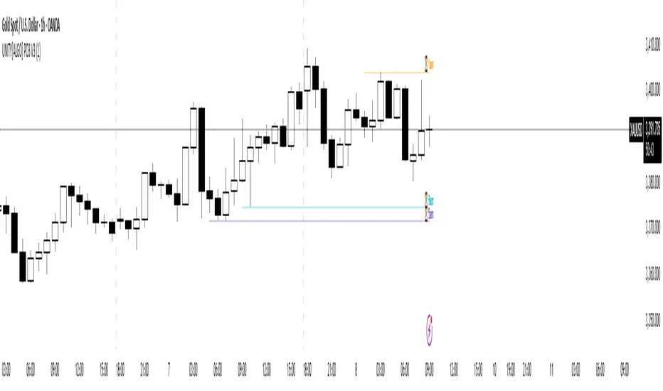
UNITY[ALGO] PO3 V3Of course. Here is a complete and professional description in English for the indicator we have built, detailing all of its features and functionalities.
Indicator: UNITY PO3 V7.2
Overview
The UNITY PO3 is an advanced, multi-faceted technical analysis tool designed to identify high-probability reversal setups based on the Swing Failure Pattern (SFP). It combines real-time SFP detection on the current timeframe with a sophisticated analysis of key institutional liquidity zones from the H4 timeframe, presenting all information in a clear, dynamic, and interactive visual interface.
This indicator is built for traders who use liquidity concepts, providing a complete dashboard of entries, targets, and invalidation levels directly on the chart.
Core Features & Functionality
1. Swing Failure Pattern (SFP) Detection (Current Timeframe)
The indicator's primary engine identifies SFPs on the chart's active timeframe with two layers of logic:
Standard SFP: Detects a classic liquidity sweep where the current candle's wick takes out the high or low of the previous candle and the body closes back within the previous candle's range.
Outside Bar SFP Logic: Intelligently analyzes engulfing candles that sweep both the high and low of the previous candle. A valid signal is only generated if the candle has a clear directional close:
Bullish Signal: If the outside bar closes higher than its open.
Bearish Signal: If the outside bar closes lower than its open.
Neutral (doji-like) outside bars are ignored to filter for indecision.
2. Comprehensive On-Chart SFP Markings
When a valid SFP is detected, a full suite of dynamic drawings appears on the chart:
Failure Line: A dashed line (red for bearish, green for bullish) marking the precise price level of the liquidity sweep.
PREMIUM ZONE (SFP Candle Wick): A transparent, colored rectangle highlighting the rejection wick of the signal candle (the upper wick for bearish SFPs, the lower wick for bullish SFPs). This zone automatically extends to the right, following the current price, until the DOL is hit.
CRT BOX (Reference Candle): A transparent box with a colored border drawn around the entire range of the candle that was swept (Candle 1). This highlights the full liquidity zone and also extends dynamically until the DOL is hit.
Dynamic Target Line: A blue dashed line marking the primary objective (the low of the signal candle for shorts, the high for longs).
The line begins with a "⏳ Target" label and extends with the current price.
Upon being touched by price, the line freezes, and its label permanently changes to "✅ Target".
Dynamic DOL (Draw on Liquidity) Line: An orange dashed line marking the invalidation level, defined as the opposite extremity of the swept candle (Candle 1).
It begins with a "⏳ dol" label and extends with the price.
Upon being touched, it freezes, and its label changes to "✅ dol".
3. Multi-Session Killzone Liquidity Levels (H4 Analysis)
The indicator automatically analyzes the H4 timeframe in the background to identify and plot key liquidity levels from three major trading sessions, based on their UTC opening times.
1am Killzone (London Lunch): Tracks the high/low of the 05:00 UTC H4 candle.
5am Killzone (London Open): Tracks the high/low of the 09:00 UTC H4 candle.
9am Killzone (NY Open): Tracks the high/low of the 13:00 UTC H4 candle.
For each of these Killzones, the indicator provides two types of analysis:
Last KZ Lines: Plots the high and low of the most recent qualifying Killzone candle. These lines are dynamic, extending with price and showing a ⏳/✅ status when touched.
Fresh Zones: A powerful feature that scans the entire available history of Killzones to find and display the closest untouched high (above the current price) and the closest untouched low (below the current price). These "Fresh" lines are also fully dynamic and provide a real-time view of the most relevant nearby liquidity targets.
4. Advanced User Settings & Chart Management
The indicator is designed for a clean and user-centric experience with powerful customization:
Show Only Last SFP: Keeps the chart clean by automatically deleting the previous SFP setup when a new one appears.
Hide SFP on DOL Reset: When checked, automatically removes all drawings related to an SFP setup the moment its invalidation level (DOL line) is touched. This leaves only active, valid setups on the chart.
Hide Consumed KZ: When checked, automatically removes any Killzone or Fresh Zone line from the chart as soon as it is touched by the price.
Independent Toggles: Every visual element—SFP signals, each of the three Killzones, and their respective "Fresh" zone counterparts—can be turned on or off independently from the settings menu for complete control over the visual display.
Z-Order Priority: All indicator drawings are rendered in front of the chart candles, ensuring they are always clearly visible and never hidden from view.
Dynamic Fib Pro by Qabas Algo🔹 Dynamic Fib Pro by Qabas Algo
Dynamic Fib Pro is an intelligent Fibonacci-based indicator that adapts to real market behavior by incorporating volatility and momentum into classic Fibonacci levels. This tool is ideal for traders who want realistic, responsive, and smart support/resistance zones rather than static levels.
⸻
🚀 Key Features:
• Adaptive Fibonacci Levels: Each level is dynamically adjusted based on current volatility and momentum strength, offering more relevant price zones.
• Smart Trend Detection: Option to auto-detect trend using SMA20 vs SMA50 crossover or pure price action logic.
• Volatility-Aware Scaling: Levels expand or contract depending on market volatility, avoiding rigid assumptions.
• Momentum-Based Adjustment: Uses range and average price to assess strength and adjust levels accordingly.
• Custom Styling: Choose from dashed, dotted, or solid lines, and control the max level displayed.
• Optional Percentage Labels: View both classic and adjusted Fibonacci % next to each level (e.g., 61.8% → 78.4%).
⸻
🎯 Use Case:
This indicator is built for discretionary traders, swing traders, and scalpers who want to:
• Identify meaningful dynamic support/resistance levels
• React to price behavior in real time
• Incorporate market volatility and strength into their strategy
⸻
⚙️ Settings Overview:
• Show Fibonacci Levels – Toggle main levels on/off
• Max Level – Limit the highest level to keep the chart clean
• Show Percentage Labels – View classic vs adjusted percentages
• Use Moving Averages – Enable SMA20/50 trend filtering
• Line Style – Choose between solid, dashed, or dotted
⸻
📌 Notes:
• Levels are calculated from the last 100 bars (High/Low range)
• Adjustments use both current volatility and 50-bar momentum strength
• The indicator updates in real time on each new bar
⸻
🧠 Created with precision by Qabas Algo — designed to make Fibonacci smarter.
If you like this tool, leave a comment or follow for more advanced indicators!

Week Window AlgorithmWeek Window Algorithm
The Week Window Algorithm is an advanced intraday trading overlay built for precision session tracking and key level visualization.
🔹 Features:
1. Time Lines
Automatically plots vertical lines 30 minutes ahead of specific London times (07, 08, 09, 13, 14, 15UK), with adjustable height in pips and custom color.
2. Session Boxes
Draws price range boxes for:
Asia (22:00–06:00 UK)
Europe AM (08:00–09:00 UK)
Europe PM (14:00–15:00 UK)
Each box auto-updates during the session and fades after 3 days. Fill color is fully customizable via settings.
3. Yesterday’s High/Low Levels
Captures and plots yesterday’s high and low at 23:00 UK. Lines extend through today and highlight first-time hits.
🛠️ Customization:
Enable/disable sessions individually
Set pip size for early lines
Choose colors for each session box and line style
🕒 Recommended Timeframes:
Optimized for 1–15 minute charts. Works best on intraday setups.

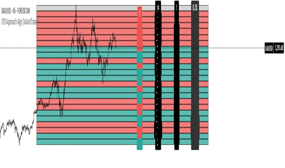
CPD Approach Algo [ValiantTrader]CPD Approach Algo Indicator Explained
This indicator, created by ValiantTrader, is a sophisticated tool for analyzing price action and market structure across different timeframes. Here's how it works and how traders use it:
Core Functionality
The CPD (Candle Price Distribution) Approach Algo divides the price range into horizontal zones and analyzes several key metrics within each zone:
Price Distribution: Shows where price has spent most time (high concentration areas)
Volume Clusters: Identifies zones with significant trading volume
Pressure Zones: Detects buying/selling pressure in specific price levels
Candle Differences: Highlights transitions between zones
How Traders Use It
1. Identifying Key Levels
The colored zones (green for buy, red for sell, gray neutral) show where price has historically reacted
Dense candle clusters indicate strong support/resistance areas
2. Volume Analysis
Volume clusters reveal where most trading activity occurred
High volume zones often act as magnets for price or reversal points
3. Pressure Detection
The pressure zones (with ↑ and ↓ arrows) show where buying or selling pressure was strongest
Helps identify potential breakout or reversal points
4. Multi-Timeframe Analysis
The custom timeframe input allows analyzing higher timeframe structure while viewing lower timeframe charts
Helps align trades with the dominant timeframe's structure
5. Transition Analysis
The delta values between zones show how price is moving between levels
Positive deltas (green) show upward momentum, negative (red) show downward
Practical Trading Applications
Support/Resistance Trading: Fade price at dense candle clusters with opposing pressure
Breakout Trading: Trade breaks from low-candle-count zones into high-volume zones
Mean Reversion: Trade returns to high-volume value areas after deviations
Trend Confirmation: Consistent pressure in one direction confirms trend strength
The indicator provides a comprehensive view of market structure by combining price, volume, and time elements across customizable timeframes, helping traders make more informed decisions about potential entries, exits, and key levels to watch.
GOD Complex Trading By QTX Algo SystemsGOD Complex Trading by QTX Algo Systems
Overview
GOD Complex Trading is a comprehensive signal engine that combines multiple QTX Algo Systems indicators into a unified framework for identifying high-confluence reversal and continuation setups. It includes dynamic entry detection, adaptive stop loss logic, multi-timeframe analysis, score-based risk scaling, and real-time trade visualization.
This script is designed for discretionary traders who want to see structured trade logic unfold directly on the chart, with visual labeling of entry type, dynamic stop loss placement, exit score computation, and key trade metrics shown in an on-chart table.
How It Works
Each trade is classified into one of four categories:
Reversal Long
Reversal Short
Continuation Long
Continuation Short
Each trade type has a distinct confluence requirement involving real-time and higher-timeframe inputs. The indicator calculates a confluence score out of 200 and determines HTF (high-timeframe) directional bias across three layers (HTF1, HTF2, HTF3), which are configurable.
QTX Indicators Used
This script integrates internal logic from the following proprietary QTX tools:
VBM (Volatility-Based Momentum) – Confirms directional bias using momentum slope and volatility increase.
VBSMI (Volatility-Based SMI) – Detects early momentum shifts via band exits and crossovers of adaptive smoothed SMI values.
SEA (Statistically Extreme Areas) – Highlights exhaustion zones using normalized volatility, smoothed range deviation, and SMI divergence.
SPB (Statistical Price Bands) – Uses volatility and trend-adjusted percentiles to define dynamic overbought/oversold zones.
COI (Continuation Opportunity Indicator) – Validates re-entry opportunities following a pullback during trend continuation.
Signal Logic – Examples
Each entry type is built from layered logic:
Reversal Long (Example)
Triggers when:
VBSMI is in dynamic oversold and crosses up
SEA level is at or below threshold (signaling statistical exhaustion)
SPB confirms recent low percentile hit
VBM and COI do not indicate trend continuation in the opposite direction
Continuation Long (Example)
Triggers when:
No recent extreme zones (SPB or SEA) are present
VBM confirms continued trend momentum
VBSMI crosses up and confirms strength
COI may confirm re-entry conditions
High-timeframe bias scores show alignment
All entries are subject to filter checks, including:
Minimum confluence score
HTF bias thresholds (HTF1, HTF2, HTF3)
Position type and trade history
Key Features
Trade Type Auto-Labeling
Each signal is labeled (“Rev Long”, “Cont Short”, etc.) directly on the chart for instant identification.
Stop Loss Visualization
Stop loss levels are calculated using a weighted average of ATR-based padding and prior swing highs/lows. Ghost lines are drawn for Add trades.
TP1 / TP2 Logic
TP1: Fires on opposite VBSMI crossover (momentum loss).
TP2: Fires when the opposite side’s reversal score exceeds a user-defined threshold.
Position Size & Risk Table
The on-chart table shows estimated trade size (based on max risk input), stop loss price, and calculated exit score. Reversal trades scale based on confluence score, while continuation trades use linear scaling.
Multi-Timeframe Confluence
The script uses three automatic higher timeframes to calculate directional bias and exit score amplification. This allows scoring logic to reflect broader trend alignment.
Add Trade Logic
The indicator detects both same-style and cross-style Add setups. Add signals are labeled and visualized, but should be used cautiously.
Auto-Close on Opposite Signal
When an opposite entry signal is triggered (e.g. Cont Short after Rev Long), the current trade is automatically considered closed, resetting tracking variables and metrics.
Additional Features
Fully bar-closed logic: no repainting or mid-bar recalculation.
High-precision control over alert triggering using bias filters and score ranges.
Dedicated alert conditions for all key trade types and TP/SL events.
Score-based position sizing using dynamic confluence score caps.
Table remains visible for a configurable number of bars after trade close.
Use Cases
Manual discretionary entries with clearly labeled setups and real-time validation
Score-based trade review and journaling using TP1/TP2 and exit score
Optimizing trade filters using alerts with HTF bias and confluence thresholds
Data-driven strategy refinement by observing which trades reach full exits
Disclaimer
This tool is provided for educational and informational purposes only. It does not guarantee any particular outcome or profitability. Always use proper risk management, backtest thoroughly, and consult a financial professional if needed.

VICI Algo-V TableVICI Trading Solutions is proud to introduce another powerful tool from our internal trading process: ALGO V ATR Table.
This streamlined, data-rich table is designed to give traders quick and easy access to key support and resistance levels using Average True Range (ATR) data—without cluttering the chart. It’s a perfect complement to our previously released ALGO V indicator, which plots significant ATR-based levels directly on the chart. While that tool is highly effective, we understand that too much on the screen can overwhelm your workspace. That’s why we developed this clean, corner-based ATR Table —so you can stay focused on execution with clarity and confidence.
How It Works:
- The table displays critical ATR levels across multiple timeframes, helping you identify areas of potential support and resistance with precision.
- Each timeframe row is color-coded to reflect its current trend state:
- 🟩 Green – Price is above the cloud and trending up .
- 🟥 Red – Price is below the cloud and trending down .
- ⬜ Gray – Price is inside the cloud and in a neutral/indecisive zone.
- The number next to a gray level shows the price that must be broken to transition to a bullish or bearish trend.
This simple color system allows for immediate insight into market structure and directional bias across multiple timeframes—without second guessing or crowding your chart.
⚠️ Important Note: Due to how TradingView handles higher time frame data, this indicator is designed to function best when applied to a 5-minute or lower time frame. We recommend adding this to your execution chart for the most accurate and responsive data.
Recommended Use:
We suggest pairing this with the original ALGO V indicator to better understand how these levels behave, especially when they appear gray (neutral). This combination provides a full-spectrum view of trend strength, key zones, and potential breakouts .
Whether you’re a scalper, day trader, or swing trader, the ALGO V ATR Table will instantly add value to your trading workflow—offering clear, concise, and actionable insight at a glance.
Algo-V Indicator Can Be Found HERE:

Harish algo for nifty and bankniftyHarish algo for nifty and banknifty
Overview
Harish Algo - Buy and Sell 11 is a powerful trading indicator designed for intraday traders, incorporating multiple technical analysis concepts to identify potential breakout and breakdown levels. It uses pivot points, exponential moving averages (EMAs), and volatility-based levels to generate buy and sell signals with visual markers for better decision-making.
Features & Functionality
✅ Pivot Points Calculation:
The indicator calculates daily pivot points along with resistance (R1) and support (S1) levels.
Helps in identifying potential reversal or breakout areas.
✅ EMA Trend Confirmation:
Uses three EMAs (21, 55, and 200) to confirm trend direction.
Ensures that buy signals align with uptrends and sell signals align with downtrends.
✅ 15-Minute Candle Analysis for Precision:
Captures the last three 15-minute closes of the previous day.
Computes an average and determines volatility-based price levels to anticipate price movements.
✅ Dynamic Buy & Sell Signals:
Bullish (Buy) Signals:
Price breaks above key resistance levels and EMAs confirm an uptrend.
Displayed as yellow (tiny) or green (small) upward triangles below candles.
Bearish (Sell) Signals:
Price drops below key support levels with EMA confirmation of a downtrend.
Displayed as fuchsia (tiny) or red (small) downward triangles above candles.
✅ Alerts for Trade Execution:
Get notified instantly with alerts when a buy or sell signal is triggered.
✅ Customizable Settings:
Modify EMA lengths and adjust parameters to fit different trading strategies.
Usage & Benefits
🔹 Helps traders identify potential entry and exit points with precision.
🔹 Reduces false signals by combining pivot points, EMAs, and price action.
🔹 Works best for intraday traders in the Indian stock markets, but can be applied to other markets as well.
🔹 Suitable for both beginners and experienced traders looking for a structured approach to trading.
How to Use
Add the indicator to your chart.
Observe the plotted pivot points, EMAs, and price levels.
Watch for triangle markers (buy/sell signals).
Use alerts to receive real-time notifications.
Combine with your own risk management strategy for best results.
🔹 Works on all timeframes but optimized for intraday trading.
Disclaimer
📢 This indicator is for educational purposes only and should not be considered financial advice. Always perform your own analysis before taking trades.

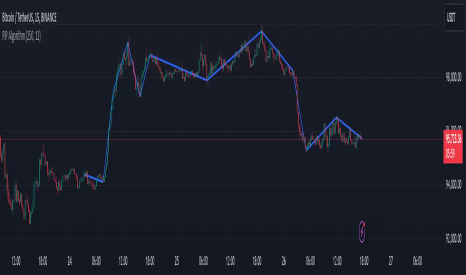
PIP Algorithm
# **Script Overview (For Non-Coders)**
1. **Purpose**
- The script tries to capture the essential “shape” of price movement by selecting a limited number of “key points” (anchors) from the latest bars.
- After selecting these anchors, it draws straight lines between them, effectively simplifying the price chart into a smaller set of points without losing major swings.
2. **How It Works, Step by Step**
1. We look back a certain number of bars (e.g., 50).
2. We start by drawing a straight line from the **oldest** bar in that range to the **newest** bar—just two points.
3. Next, we find the bar whose price is *farthest away* from that straight line. That becomes a new anchor point.
4. We “snap” (pin) the line to go exactly through that new anchor. Then we re-draw (re-interpolate) the entire line from the first anchor to the last, in segments.
5. We repeat the process (adding more anchors) until we reach the desired number of points. Each time, we choose the biggest gap between our line and the actual price, then re-draw the entire shape.
6. Finally, we connect these anchors on the chart with red lines, visually simplifying the price curve.
3. **Why It’s Useful**
- It highlights the most *important* bends or swings in the price over the chosen window.
- Instead of plotting every single bar, it condenses the information down to the “key turning points.”
4. **Key Takeaway**
- You’ll see a small number of red line segments connecting the **most significant** points in the price data.
- This is especially helpful if you want a simplified view of recent price action without minor fluctuations.
## **Detailed Logic Explanation**
# **Script Breakdown (For Coders)**
//@version=5
indicator(title="PIP Algorithm", overlay=true)
// 1. Inputs
length = input.int(50, title="Lookback Length")
num_points = input.int(5, title="Number of PIP Points (≥ 3)")
// 2. Helper Functions
// ---------------------------------------------------------------------
// reInterpSubrange(...):
// Given two “anchor” indices in `linesArr`, linearly interpolate
// the array values in between so that the subrange forms a straight line
// from linesArr to linesArr .
reInterpSubrange(linesArr, segmentLeft, segmentRight) =>
float leftVal = array.get(linesArr, segmentLeft)
float rightVal = array.get(linesArr, segmentRight)
int segmentLen = segmentRight - segmentLeft
if segmentLen > 1
for i = segmentLeft + 1 to segmentRight - 1
float ratio = (i - segmentLeft) / segmentLen
float interpVal = leftVal + (rightVal - leftVal) * ratio
array.set(linesArr, i, interpVal)
// reInterpolateAllSegments(...):
// For the entire “linesArr,” re-interpolate each subrange between
// consecutive breakpoints in `lineBreaksArr`.
// This ensures the line is globally correct after each new anchor insertion.
reInterpolateAllSegments(linesArr, lineBreaksArr) =>
array.sort(lineBreaksArr, order.asc)
for i = 0 to array.size(lineBreaksArr) - 2
int leftEdge = array.get(lineBreaksArr, i)
int rightEdge = array.get(lineBreaksArr, i + 1)
reInterpSubrange(linesArr, leftEdge, rightEdge)
// getMaxDistanceIndex(...):
// Return the index (bar) that is farthest from the current “linesArr.”
// We skip any indices already in `lineBreaksArr`.
getMaxDistanceIndex(linesArr, closeArr, lineBreaksArr) =>
float maxDist = -1.0
int maxIdx = -1
int sizeData = array.size(linesArr)
for i = 1 to sizeData - 2
bool isBreak = false
for b = 0 to array.size(lineBreaksArr) - 1
if i == array.get(lineBreaksArr, b)
isBreak := true
break
if not isBreak
float dist = math.abs(array.get(linesArr, i) - array.get(closeArr, i))
if dist > maxDist
maxDist := dist
maxIdx := i
maxIdx
// snapAndReinterpolate(...):
// "Snap" a chosen index to its actual close price, then re-interpolate the entire line again.
snapAndReinterpolate(linesArr, closeArr, lineBreaksArr, idxToSnap) =>
if idxToSnap >= 0
float snapVal = array.get(closeArr, idxToSnap)
array.set(linesArr, idxToSnap, snapVal)
reInterpolateAllSegments(linesArr, lineBreaksArr)
// 3. Global Arrays and Flags
// ---------------------------------------------------------------------
// We store final data globally, then use them outside the barstate.islast scope to draw lines.
var float finalCloseData = array.new_float()
var float finalLines = array.new_float()
var int finalLineBreaks = array.new_int()
var bool didCompute = false
var line pipLines = array.new_line()
// 4. Main Logic (Runs Once at the End of the Current Bar)
// ---------------------------------------------------------------------
if barstate.islast
// A) Prepare closeData in forward order (index 0 = oldest bar, index length-1 = newest)
float closeData = array.new_float()
for i = 0 to length - 1
array.push(closeData, close )
// B) Initialize linesArr with a simple linear interpolation from the first to the last point
float linesArr = array.new_float()
float firstClose = array.get(closeData, 0)
float lastClose = array.get(closeData, length - 1)
for i = 0 to length - 1
float ratio = (length > 1) ? (i / float(length - 1)) : 0.0
float val = firstClose + (lastClose - firstClose) * ratio
array.push(linesArr, val)
// C) Initialize lineBreaks with two anchors: 0 (oldest) and length-1 (newest)
int lineBreaks = array.new_int()
array.push(lineBreaks, 0)
array.push(lineBreaks, length - 1)
// D) Iteratively insert new breakpoints, always re-interpolating globally
int iterationsNeeded = math.max(num_points - 2, 0)
for _iteration = 1 to iterationsNeeded
// 1) Re-interpolate entire shape, so it's globally up to date
reInterpolateAllSegments(linesArr, lineBreaks)
// 2) Find the bar with the largest vertical distance to this line
int maxDistIdx = getMaxDistanceIndex(linesArr, closeData, lineBreaks)
if maxDistIdx == -1
break
// 3) Insert that bar index into lineBreaks and snap it
array.push(lineBreaks, maxDistIdx)
array.sort(lineBreaks, order.asc)
snapAndReinterpolate(linesArr, closeData, lineBreaks, maxDistIdx)
// E) Save results into global arrays for line drawing outside barstate.islast
array.clear(finalCloseData)
array.clear(finalLines)
array.clear(finalLineBreaks)
for i = 0 to array.size(closeData) - 1
array.push(finalCloseData, array.get(closeData, i))
array.push(finalLines, array.get(linesArr, i))
for b = 0 to array.size(lineBreaks) - 1
array.push(finalLineBreaks, array.get(lineBreaks, b))
didCompute := true
// 5. Drawing the Lines in Global Scope
// ---------------------------------------------------------------------
// We cannot create lines inside barstate.islast, so we do it outside.
array.clear(pipLines)
if didCompute
// Connect each pair of anchors with red lines
if array.size(finalLineBreaks) > 1
for i = 0 to array.size(finalLineBreaks) - 2
int idxLeft = array.get(finalLineBreaks, i)
int idxRight = array.get(finalLineBreaks, i + 1)
float x1 = bar_index - (length - 1) + idxLeft
float x2 = bar_index - (length - 1) + idxRight
float y1 = array.get(finalCloseData, idxLeft)
float y2 = array.get(finalCloseData, idxRight)
line ln = line.new(x1, y1, x2, y2, extend=extend.none)
line.set_color(ln, color.red)
line.set_width(ln, 2)
array.push(pipLines, ln)
1. **Data Collection**
- We collect the **most recent** `length` bars in `closeData`. Index 0 is the oldest bar in that window, index `length-1` is the newest bar.
2. **Initial Straight Line**
- We create an array called `linesArr` that starts as a simple linear interpolation from `closeData ` (the oldest bar’s close) to `closeData ` (the newest bar’s close).
3. **Line Breaks**
- We store “anchor points” in `lineBreaks`, initially ` `. These are the start and end of our segment.
4. **Global Re-Interpolation**
- Each time we want to add a new anchor, we **re-draw** (linear interpolation) for *every* subrange ` [lineBreaks , lineBreaks ]`, ensuring we have a globally consistent line.
- This avoids the “local subrange only” approach, which can cause clustering near existing anchors.
5. **Finding the Largest Distance**
- After re-drawing, we compute the vertical distance for each bar `i` that isn’t already a line break. The bar with the biggest distance from the line is chosen as the next anchor (`maxDistIdx`).
6. **Snapping and Re-Interpolate**
- We “snap” that bar’s line value to the actual close, i.e. `linesArr = closeData `. Then we globally re-draw all segments again.
7. **Repeat**
- We repeat these insertions until we have the desired number of points (`num_points`).
8. **Drawing**
- Finally, we connect each consecutive pair of anchor points (`lineBreaks`) with a `line.new(...)` call, coloring them red.
- We offset the line’s `x` coordinate so that the anchor at index 0 lines up with `bar_index - (length - 1)`, and the anchor at index `length-1` lines up with `bar_index` (the current bar).
**Result**:
You get a simplified representation of the price with a small set of line segments capturing the largest “jumps” or swings. By re-drawing the entire line after each insertion, the anchors tend to distribute more *evenly* across the data, mitigating the issue where anchors bunch up near each other.
Enjoy experimenting with different `length` and `num_points` to see how the simplified lines change!
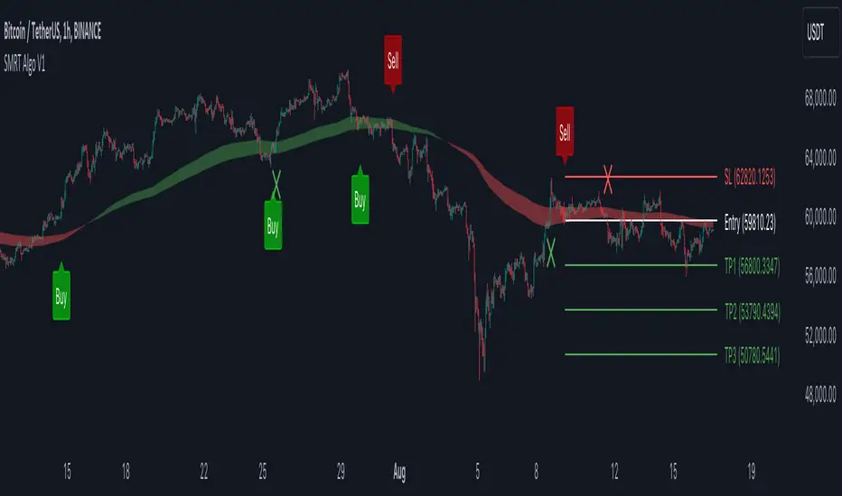
V1 [SMRT Algo]SMRT Algo V1 is a versatile trading indicator designed to provide traders with clear and actionable signals.
The system includes both standard buy/sell signals and confirmed buy/sell signals, denoted by an 'x', which appear after a signal is validated. Traders have the flexibility to enable or disable the confirmed signals based on their trading strategy preferences.
The combination of standard and confirmed buy/sell signals ensures that traders receive both initial alerts and validated signals, thereby enhancing the accuracy and reliability of trade entries. This dual-signal approach helps filter out false signals, providing an additional layer of security for traders.
Core Features:
Standard Signals: These signals are generated based on a pullback logic, where a signal is printed when the price returns to the average price level (the pullback zone) and starts to move away, indicating a potential trend continuation or reversal.
Confirmed Signals ('x'): These appear after the initial signal, providing additional validation and reducing false signals. This feature is particularly useful for traders who seek a higher level of confirmation before entering a trade.
MA Filter: The Moving Average (MA) Filter is a critical component that filters trades to ensure that only those aligned with the prevailing trend are considered. This filter helps in eliminating signals that go against the primary market trend, thereby increasing the probability of successful trades.
Dynamic Support and Resistance (S/R): The Dynamic S/R feature uses background plots to denote zones of support and resistance that are continuously updated based on market movements. These zones are used as part of the signal generation process, helping to identify key levels where price action may reverse or accelerate.
Take Profit (TP) and Stop Loss (SL) Levels: Each trade signal is accompanied by predefined TP and SL levels, offering traders clear guidance on potential exit points. TP levels are structured to provide different risk-reward ratios (e.g., TP1 for 1:1, TP2 for 1:2, TP3 for 1:3), allowing for flexible trade management according to individual risk tolerance and market conditions.
The MA Filter further refines this process by aligning trades with the prevailing market trend. By using a moving average as a filter, the system ensures that signals are only generated in the direction of the trend, reducing the likelihood of counter-trend trades that often carry higher risks. This feature is particularly beneficial in trending markets where maintaining the direction of trades with the overall trend increases the probability of success.
Dynamic Support and Resistance (S/R) zones play a crucial role in the indicator's signal generation and trade management strategies. These zones are not static but adjust in real-time based on market conditions, providing traders with up-to-date information on critical price levels. The integration of dynamic S/R with the signal generation process helps in identifying potential reversal or acceleration points, making it a valuable tool for both trend-following and reversal strategies.
Input Settings:
Show Confirmed Signals: Turning this on will show the ‘x’ on the chart, meaning a signal is confirmed.
Trend Bar Color: Turning this on will result in the signal candle being colored green for buy, and red for sell.
RSI Filter: Turning this feature off will result in not requiring the RSI condition to be met in order for signals to be generated. Turning this off will result in a higher frequency of signals.
X-Bar Range: How far back the indicator will look for signals. Increasing this value will lead to more signals generated, decreasing will lead to less signals.
MA Filter: Turning this on will result in only buy trades being printed when price is above the MA cloud, the opposite for sells. Turning this off will increase in more signals.
Dynamic S/R: This is the trend cloud that is shown on screen. It acts as a dynamic support/resistance as it moves along with price. This zone often acts as a retest (support) zone and is also where signals are often generated. It can be turned on/off visually.
TP/SL: The take profit & stop loss zones can be turned on/off. The size of TP/SL can also be adjusted by increasing or decreasing the multiplier and length values.
These components are not isolated features but work together to create a cohesive and comprehensive trading system. The standard and confirmed signals provide timely and validated entry points, while the MA Filter ensures these entries align with the broader trend. The dynamic S/R zones add another layer of analysis, highlighting critical levels that can influence price movements. Together, these features offer a well-rounded view of the market, enabling traders to make more informed and strategic decisions. The inclusion of TP and SL levels integrates risk management into every trade, making the system not only a tool for identifying trades but also for managing them effectively.
The SMRT Algo Suite offers a comprehensive set of tools and features that extend beyond the capabilities of standard or open-source indicators, providing significant additional value to users.
Advanced Customization: Users can customize various aspects of the indicator, such as toggling the confirmation signals on or off and adjusting the parameters of the MA Filter. This customization enhances the adaptability of the tool to different trading styles and market conditions.
Enhanced Market Understanding: The combination of pullback logic, dynamic S/R zones, and MA filtering offers traders a nuanced understanding of market dynamics, helping them make more informed trading decisions.
Unique Features: The specific combination of pullback logic, dynamic S/R, and multi-level TP/SL management is unique to SMRT Algo V1, offering features that are not readily available in standard or open-source indicators.
Educational and Support Resources: As with other products in the SMRT Algo suite, this indicator comes with comprehensive educational resources and access to a supportive trading community, as well as 24/7 Discord support.
The educational resources and community support included with SMRT Algo ensure that users can maximize the indicators’ potential, offering guidance on best practices and advanced usage.
SMRT Algo believe that there is no magic indicator that is able to print money. Indicator toolkits provide value via their convinience, adaptibility and uniqueness. Combining these items can help a trader make more educated; less messy, more planned trades and in turn hopefully help them succeed.
RISK DISCLAIMER
Trading involves significant risk, and most day traders lose money. All content, tools, scripts, articles, and educational materials provided by SMRT Algo are intended solely for informational and educational purposes. Past performance is not indicative of future results. Always conduct your own research and consult with a licensed financial advisor before making any trading decisions.
Reversal Finder [SMRT Algo]The Reversal Indicator is designed for traders who use contrarian strategies, focusing on identifying potential reversal points in the market. This indicator leverages mean and deviation calculations, along with bar pattern movements, to provide insights into price movements and potential turning points.
Features:
The Reversal Indicator is tailored for contrarian trading, which involves taking positions against the trend to capitalize on potential reversals. This approach is inherently riskier, as it aims to identify precise highs and lows in the market.
Configurable Sensitivity: Traders can adjust the sensitivity of the indicator, which determines how many confirmation candles are required before a signal is generated. Higher sensitivity values mean more confirmation candles, resulting in later but more reliable signals. This feature allows traders to balance between early entries and signal accuracy.
Separate Buy & Sell Sensitivities: Buy and sell sensitivities can be adjusted separately which provides greater flexibility, enabling traders to fine-tune the indicator based on market conditions or personal trading preferences.
Reversal Bands: The indicator features color-coded bands (green, yellow, red) that represent different levels of price overextension. The dynamic nature of these bands, which adjust based on real-time market data, provides a constantly updated visual representation of potential reversal zones.
- Green Band: Indicates the initial phase where price is starting to get overextended.
- Yellow Band: Suggests a moderate level of overextension.
- Red Band: Signals a high likelihood of reversal due to significant overextension.
Signal Generation: The indicator only searches for buy or sell signals when the price enters these reversal bands, thereby focusing on zones with a higher probability of a reversal.
Take Profit (TP) & Stop Loss (SL) Features: The indicator includes predefined TP and SL levels, calculated based on a risk-to-reward ratio with respect to the stop loss. For instance, TP1 corresponds to a 1:1 ratio, up to TP3, allowing traders to manage risk effectively and set realistic profit targets.
Band-Based Take Profit: In addition to standard TP levels, traders can use the reversal bands themselves as take profit zones, targeting the green, yellow, or red areas to close trades. This dual-layered approach provides more nuanced trade management options.
Alert System: The indicator allows traders to set alerts for when signals are generated, ensuring they do not miss potential trading opportunities.
A signal is generate when we have x-consecutive bullish/bearish bars for a buy or sell signal respectively. This is what the 'Sensitivity' input controsl for in the settings. A signal is only generated when price enters the deviation bands, as those are areas where a reversal is of higher probability.
The Reversal indicator uses mean and deviation calculations, which are fundamental to the Reversal Indicator, providing a statistical baseline for identifying overextended price movements. By measuring how far price deviates from its mean, the indicator identifies conditions where a reversal is more likely. This statistical foundation ensures that the signals are based on objective data, rather than subjective judgment.
The integration of bar pattern analysis with mean and deviation calculations allows the indicator to add a layer of context to the raw data. Bar patterns are used to confirm potential reversals by analyzing the formation of candles and the overall structure of the price action. This component enhances the accuracy of signals by ensuring they are not only statistically significant but also contextually relevant.
The Reversal Indicator’s unique sensitivity adjustment feature allows traders to fine-tune the responsiveness of the signals. This flexibility means the indicator can be adapted to various market conditions, enhancing its utility across different trading environments. The separate adjustment for buy and sell sensitivities further allows traders to customize the indicator based on their specific trading strategies, whether they are more conservative or aggressive in their approach.
The Reversal Indicator's unique combination of statistical and pattern-based analysis, customizable settings, and dynamic real-time components offers significant added value compared to standard indicators.
The SMRT Algo Suite, which the Reversal Finder is a part of, offers a comprehensive set of tools and features that extend beyond the capabilities of standard or open-source indicators, providing significant additional value to users.
What you also get with the SMRT Algo Suite:
Advanced Customization: Users can customize various aspects of the indicator, such as toggling the confirmation signals on or off and adjusting the parameters of the MA Filter. This customization enhances the adaptability of the tool to different trading styles and market conditions.
Enhanced Market Understanding: The combination of pullback logic, dynamic S/R zones, and MA filtering offers traders a nuanced understanding of market dynamics, helping them make more informed trading decisions.
Unique Features: The specific combination of pullback logic, dynamic S/R, and multi-level TP/SL management is unique to SMRT Algo, offering features that are not readily available in standard or open-source indicators.
Educational and Support Resources: As with other tools in the SMRT Algo suite, this indicator comes with comprehensive educational resources and access to a supportive trading community, as well as 24/7 Discord support.
The educational resources and community support included with SMRT Algo ensure that users can maximize the indicators’ potential, offering guidance on best practices and advanced usage.
SMRT Algo believe that there is no magic indicator that is able to print money. Indicator toolkits provide value via their convinience, adaptibility and uniqueness. Combining these items can help a trader make more educated; less messy, more planned trades and in turn hopefully help them succeed.
RISK DISCLAIMER
Trading involves significant risk, and most day traders lose money. All content, tools, scripts, articles, and educational materials provided by SMRT Algo are intended solely for informational and educational purposes. Past performance is not indicative of future results. Always conduct your own research and consult with a licensed financial advisor before making any trading decisions.

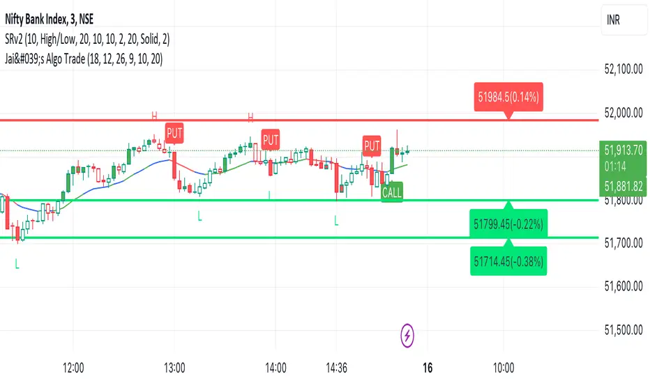
Jai's Algo SignalsOverview:
Jai's Algo Trade Indicator is a sophisticated trading tool designed to enhance your trading strategy by combining the strengths of two widely-used technical indicators: the Exponential Moving Average (EMA) and the Moving Average Convergence Divergence (MACD). This synergy provides a robust framework for identifying market trends and potential trade opportunities, making it ideal for both novice and experienced traders.
Justification for Combining EMA and MACD:
The EMA is a trend-following indicator that smooths out price data to highlight the direction of the trend, while the MACD is a momentum oscillator that reveals changes in the strength, direction, momentum, and duration of a trend. By integrating these two indicators, Jai's Algo Trade Indicator offers a comprehensive view of market conditions, allowing traders to make more informed decisions based on both trend direction and momentum.
How It Works:
Exponential Moving Average (EMA):
Calculation: The EMA is calculated using a user-defined period (default: 13). This moving average gives more weight to recent prices, making it responsive to new information.
Visualization: The EMA line is plotted on the chart and dynamically changes color: green when the price is above the EMA, red when below, and blue when the price is at the EMA.
Moving Average Convergence Divergence (MACD):
Calculation: The MACD is computed using three parameters: fast length (default: 12), slow length (default: 26), and signal smoothing (default: 9). The MACD line, signal line, and histogram are plotted to show the relationship between two moving averages of a security’s price.
Histogram: The MACD histogram is color-coded to indicate bullish (green), bearish (red), and neutral (gray) conditions, providing visual cues for momentum changes.
Impulse System:
Bar Colors: Bars are colored based on impulse conditions:
Green bars for bullish conditions (price above EMA and MACD histogram > 0).
Red bars for bearish conditions (price below EMA and MACD histogram < 0).
Blue bars for neutral conditions.
Trade Signals:
Buy Signal: A buy (call) signal is generated when a bullish candle crosses and closes above the EMA.
Sell Signal: A sell (put) signal is generated when a bearish candle crosses and closes below the EMA.
Visualization: Signals are displayed as green "BUY" labels below the bars and red "SELL" labels above the bars, providing clear entry and exit points.
How to Use:
Input Parameters:
Customize the EMA length, MACD fast length, slow length, and signal smoothing to fit your trading strategy and timeframe.
Visual Analysis:
Monitor the color-coded EMA line and histogram to understand the current market trend and momentum.
Use the bar colors to quickly identify bullish, bearish, and neutral conditions.
Trade Signals:
Follow the "BUY" and "SELL" signals to execute trades based on the indicator's analysis.
Combine these signals with other analysis techniques and risk management practices for optimal results.
Ideal For:
Traders looking to leverage a combination of trend-following and momentum indicators for more accurate trade entries and exits.
Those who want a clear and visual representation of market conditions to aid in their decision-making process.
Conclusion:
Jai's Algo Trade Indicator integrates the EMA and MACD to provide a powerful and comprehensive trading tool. By combining trend and momentum analysis, this indicator helps traders to make more informed decisions, enhancing their trading performance and confidence.
Han Algo - Moving average strategyHan Algo Indicator Strategy Description
Overview:
The Han Algo Indicator is designed to identify trend directions and signal potential buy and sell opportunities based on moving average crossovers. It aims to provide clear signals while filtering out noise and minimizing false signals.
Indicators Used:
Moving Averages:
200 SMA (Simple Moving Average): Used as a long-term trend indicator.
100 SMA: Provides a medium-term perspective on price movements.
50 SMA: Offers insights into shorter-term trends.
20 SMA: Provides a very short-term perspective on recent price actions.
Trend Identification:
The indicator identifies the trend based on the relationship between the closing price (close) and the 200 SMA (ma_long):
Uptrend: When the closing price is above the 200 SMA.
Downtrend: When the closing price is below the 200 SMA.
Sideways: When the closing price is equal to the 200 SMA.
Buy and Sell Signals:
Buy Signal: Generated when transitioning from a downtrend to an uptrend (buy_condition):
Displayed as a green "BUY" label above the price bar.
Sell Signal: Generated when transitioning from an uptrend to a downtrend (sell_condition):
Displayed as a red "SELL" label below the price bar.
Signal Filtering:
Signals are filtered to prevent consecutive signals occurring too closely (min_distance_bars parameter):
Ensures that only significant trend reversals are captured, minimizing false signals.
Visualization:
Background Color:
Changes to green for uptrend and red for downtrend (bgcolor function):
Provides visual cues for current market sentiment.
Usage:
Traders can customize the indicator's parameters (long_term_length, medium_term_length, short_term_length, very_short_term_length, min_distance_bars) to align with their trading preferences and timeframes.
The Han Algo Indicator helps traders make informed decisions by highlighting potential trend reversals and aligning with market trends identified through moving average analysis.
Disclaimer:
This indicator is intended for educational purposes and as a visual aid to support trading decisions. It should be used in conjunction with other technical analysis tools and risk management strategies.

[FXAN] 77 Cygni Algorithm (Swing Trading)⚜️ FXAN CYGNI INDICATORS ORIGINALITY
Originality comes from proprietary formula we use to measure the relationship between Volume and Price Volatility in relation to overall current market positioning in developing Volume Profile and multiple custom period Volume Profiles. We combine that with our own approach to measure price velocity in correlation to average daily/weekly/monthly ranges of the given market.
The relationship between current volume and price volatility gives us information about how much the volume that is currently coming into the market affects the price movement (volatility) and which side is more dominant/involved in the market (Buyers/Sellers). We call this the "Volume Impact" factor.
This information is then compared in relation to the overall current market positioning in developing Volume Profile and Multiple custom period Volume Profiles. We have created a rating system based on current price positioning in relation to the Volume Profile. Volume profile consists of different volume nodes, high volume nodes where we consider market interest to be high (a lot of transactions - High Volume) and low volume nodes where we consider market interest to be low (not a lot of transactions - Low Volume). We call this the current "Market Interest" factor.
We combine this information with our own approach to measure price velocity in correlation to the higher-timeframe price ranges. Calculation is done by measuring current ranges of market movement in correlation to average daily/weekly/monthly ranges. We call this "Price Velocity" factor.
This approach was applied to develop key components of our Tradingview Indicators, we've simplified some of the calculations and made them easy to use by programming them to display buying/selling volume pressure with colors.
In addition to our own proprietary formulas and criterias to measure volume impact on price, we've also used an array of indicators that measure the percentage change in volume over custom specified periods of time, including custom period ranged Volume Profile, Developing VA, Accumulation/Distribution (A/D Line), Volume Rate of Change (VROC), Volume Price Trend (VPT) - all of them with of course fine-tuned settings to fit the purpose in the overall calculation.
Reasons for multiple indicator use:
Custom period ranged Volume Profiles: To determine current interest of market participants. Used for "Market Interest"
Developing VA: To determine current fair price of the market (value area). Used for "Market Interest".
Accumulation/Distribution (A/D Line): Helping to gauge the strength of buying and selling pressure. Used for "Volume Impact"
Volume Rate of Change (VROC): To give us information about percentage change in volume. Used for "Volume Impact"
Volume Price Trend (VPT): To help identify potential trends. Used for "Volume Impact".
Average True Range (ATR): Used for measuring volatility. Used for "Volume Impact" and "Price Velocity".
Average Daily Range (ADR): Used for measuring average market price movement. Used for "Price Velocity".
How it all works together:
"Volume Impact" factor tells us the influence of incoming market volume on price movement. This information alongside the overall market positioning information derived from "Market Interest" factor combined with information about speed and direction relative to higher-timeframe price ranges frin "Price Velocity.
This is the basis of our proprietary developed Volume Dynamics analysis approach
"Volume Impact" x "Market Interest" x "Price Velocity"
Combining this factors together gives a good overall understanding of which side is currently more involved in the market to gauge the direction ("Volume Impact"), where the market is currently positioned to gauge the context ("Market Interest") and what the current market's momentum to improve the timing of our trades ("Price Velocity"). This increases our probabilities for successful trades, executed with good timing.
To simplify - our indicators will always analyze the volume behind every price movement and rate those movements based on the relationship between movement distance and volume behind it through an array of criterias and rate them.
Colors displayed by the indicators will be a result of that, suggesting which side of the market (Buyers or sellers) is currently more involved in the market, aiming to increase the probabilities for profitable trades. With the help of our indicators you have deep volume analysis behind price movements done without looking at anything else then indicator components.
🔷 OVERVIEW
Cygni 77 Algorithm is a TradingView indicator designed to help determine higher timeframe market context and long-term market sentiment and trends. It analyzes the underlying volume behind market movements and colors the candles with the help of formulas that include technical analysis and market price action. It caters to traders looking for swing trading setups or additional perspectives for day trading sentiment.
🔷 KEY FEATURES
▊ Candle Coloring
▊ Dynamic Support & Resistance Lines
▊ Dots | Above and below the candles
▊ Colored Bar | on the bottom of the chart
🔷 HOW DOES IT WORK?
□ Candle colors will indicate the general market trend from the technical analysis perspective. The calculation for this component uses price action concepts and segments from technical analysis, for example, candle/price structural breaks. Volume is not used for calculations of this component.
□ Dynamic Support & Resistance Lines indicate the current market structure from the technical analysis perspective. The calculation uses pure price action and structural analysis of the current market movements.
□ Candle Dots show what are the mid-term volume dynamics in the market by referencing the daily average price weighted by volume with the periods ranging from days to weeks. Candle Dots suggest what is the likely direction of the market's trend from the mid-term perspective. If the market is bullish, you’ll see the green dots printed below the candles, and if the market is bearish, the dots will color red and print above the candles.
□ Colored Bar analyzes long-term volume dynamics and the market's price action for the past three to six weeks, referencing average price weighted by volume. This makes it much less sensitive than the Candle Dots, so the colors won't change that often. If the market is bullish, you’ll see the green bars, and if the market is bearish, the bars will color red.
🔷 HOW TO USE IT?
□ In general, we look for areas where all components are in sync. These are valid trading signals (refer to the usage example below).
□ If all components are not in sync, we should look for at least two of them to be in sync, while one of them must be the Colored Bar.
□ Candle Colors: Looking for longs when the candles are green and looking for shorts when the colors are red
□ Dynamic Support & Resistance Lines: Used for placing entries and stop-loss limits. Using retest of the line for entry and placing the stop-loss beyond it. Or if we're entering based on other components, we can use the line to place the stop-loss beyond it.
□ Candle Dots: Looking to trade in the direction of the color. If the market is bullish, you’ll see the green dots, and if the market is bearish, the dots will color red.
□ Colored Bar: Most important component of this indicator, we favor trading in the direction suggested by this component. Additional confirmation of other components is a bonus. Colors here don't change that often, but once they do - it usually signals a long-term trend shift. Green color suggests a bullish market, trading long. Red color suggests bearish market, trading short.
🔷 COMBINING THE COMPONENTS
Each component of the indicator serves its own purpose and analyzes the market from its own perspective and with its own custom settings and formulas. The calculation of the individual component is done independently from the calculation of the other components. Once all of them align, we can execute trades with an edge as it signals that different aspects of volume and price analysis line up for the trading opportunity.
-Candle Colors performs technical analysis for you by displaying the colors of a favorable market direction based on the market's current technical structure.
- Dynamic Support & Resistance Lines are used for placing your entry/exit limit orders.
-Candle Dots are used to determine the favorable direction of the market based on Daily Volume Dynamics, with custom timeframe settings ranging from a couple of days to a couple of weeks.
-The Colored Bar is used to gauge the overall favorable trading direction based on Daily Volume Dynamics with custom timeframe settings ranging from 3 to 6 weeks.
It's important to combine the components to increase the probability of success - here's how you should look for a trade:
1. Assess the current most favorable market direction by referencing the Colored Bar. Look for longs if it’s green and for shorts if it’s red
2. Look for the Candle Dots to align with the Colored Bar, look for longs if it’s green and for shorts if it’s red
3. Look for the Candle Colors to align with the Colored Bar. Look for longs if it’s green and for shorts if it’s red
4. Place your SL level beyond the currently developing Support/Resistance line to protect your positions and look for exits once the colors change.
A valid example of the trade would be:
- Colored Bar is green, indicating the favorable trading directions is long
- Candle Dots are green, indicating the favorable trading directions is long
- Candle Colors are green, indicating the market structure is favorable to enter your positions
📊 USAGE EXAMPLE
