Red and Green Ignored Bar by Oliver VelezOn this occasion I present a script that detects Ignored Red Candles and Ignored Green Candles, basically it is a Price Action event that indicates a possible continuation of the current trend and gives the opportunity to climb it with a Very tight risk, before delving into detail I would like to leave this note:
Note: the detection of this event does not guarantee that the signal will be good, the trader must have the ability to determine its quality based on aspects such as trend, maturity, support / resistance levels, expansion / contraction of the market, risk / benefit, etc, if you do not have knowledge about this you should not use this indicator since using it without a robust trading plan and experience could cause you to partially or totally lose your money, if this is your case you should train before If you try to extract money from the market, this script was created to be another tool in your trading plan in order to configure the rules at your discretion, execute them consistently and have AUTOMATIC ALERTS when the event occurs, which is where I find more value because you can have many instruments waiting for the event to be generated, in the time frame you want and without having to observe the mer When the alert is generated, the Trader should evaluate the quality of the alert and define whether or not to execute it (higher timeframes, they can give you more time to execute the operation correctly).
Let's continue….
This event was created by Oliver Velez recognized trader / mentor of price action, the event has a very interesting particularity since it allows to take a position with a very limited risk in trend movements, this achieves favorable operations of good ratio and small losses when taking An adjusted risk, if the trade works, a good ratio is quickly achieved and we agree with a key point in the “Keep small losses and big profits” trading, this makes it easier to have a positive mathematical hope when your level of Success is not very high, so leave you in the field of profitability.
THE EVENT:
The event has a bullish configuration (Ignored Red Candle) and a bearish configuration (Ignored Green Candle), below I detail the “Hard” rules (later I explain why “Hard”):
1- Last 3 bars have to be GREEN-RED-GREEN (possible bullish configuration) or RED-GREEN-RED (possible bearish configuration), the first bar is called Control Bar, the second is called Ignored Bar and the third Signal Bar as shown in the following image:
2- Be in a trend determined by simple moving averages (Slow of 20 periods and Fast of 8 periods), as a general rule you can take the direction of MA20 but the Trader has to determine if there is a trend movement or not.
3- Control bar of good range, little tail and with a body greater than 55%.
4- Ignored bar preferably narrow range, little tail and that is located in the upper 1/3 of the control bar.
5- Signal bar cannot override the minimum of the ignored bar.
6- Activation / Confirmation of event by means of signal bar in overcoming the body of the ignored bar.
Some examples of ignored bars (with “Hard” and “Flexible” rules):
Features and configuration of the indicator:
To access the indicator settings, press the wheel next to the indicator name VVI_VRI "Configuration options".
- Operation mode (Filtering Type):
• Filtering Complete: all filters activated according to the configuration below.
• Without Filtering: all filters deactivated, all VRI / VVI are displayed without any selection criteria.
• Trend Filter only: shows only VRI / VVI that are in accordance with what is set in “Trend Settings”
- Configuration Moving Averages:
• See Slow Media: slow moving average display with direction detection and color change.
• See Fast Media: display of fast moving average with direction detection and color change.
• Type: possibility to choose the type of media: DEMA, EMA, HullMA, SMA, SSMA, SSMA, TEMA, TMA, VWMA, WMA, ZEMA)
• Period: number of previous bars.
• Source: possibility to choose the type of source, open, close, high, low, hl2 hlc3, ohlc4.
• Reaction: this configuration affects the color change before a change of direction, 1 being an immediate reaction and higher values, a more delayed reaction obtaining les false "changes of direction", a value of 3 filters the direction quite well.
- Trend Configuration
• Uptrend Condition P / VRI: possibility to select any of these conditions:
o Bullish MA direction
o Quick bullish MA direction
o Slow and fast bullish MA direction
o Price higher than slow MA
o Price higher than fast MA
o Price higher than slow and fast MA
o Price higher than slow MA and bullish direction
o Price higher than fast MA and bullish direction
o Price higher than slow, fast MA and bullish direction
o No condition
• Condition P / VVI bear trend: possibility of selecting any of these conditions:
o Slow bearish MA direction
o Fast bearish MA direction
o Slow and fast bearish MA direction
o Price less than slow MA
o Price less than fast MA
o Price less than slow and fast MA
o Price lower than slow MA and bearish direction
o Price less than fast MA and bearish direction
o Price less than slow, fast MA and bearish direction
o No condition
- Control bar configuration
• Minimum body percentage%: possibility to select what body percentage the bar must have.
• Paint control bar: when selected, paint the control bar.
• See control bar label: when selected, a label with the legend BC is plotted.
- Configuration bar ignored
• Above X% of the control bar: possibility to select above what percentage of the control bar the ignored bar must be located.
• Paint ignored bar: when selected, paint the ignored bar.
- Signal bar configuration
• You cannot override the minimum of the ignored bar: when selected, the condition is added that the signal bar cannot override the minimum of the ignored bar.
• Paint signal bar: when selected, paint the signal bar.
• See arrow: when selected it shows the direction arrow of the possible movement.
• See bear and arrow: when selected it shows bear and arrow label
• See bull and arrow: when selected it shows bull and arrow label
The following image shows the ignored bar and painted signal:
- Take profit / loss
The profit / loss taking varies depending on the trader and its risk / monetary plan, the proposal is a recommendation based on the nature of the event that is to have a small risk unit (stop below the minimum of the ignored bar), look for objectives in ratios greater than 2: 1 and eliminate the risk in 1: 1 by taking the stop to BE, all parameters are configurable and are the following:
• See recommended stop loss and take profit: trace the levels of Stop, BE, TP1 and TP2, as well as their prices to know them quickly based on the assumed risk
• To: select which event you want to draw the SL and TP (VRI, VVI)
• Extend stop loss line x bars: allows extending the stop line by x number of bars
• Extend take profit line x bars: allows extending the stop line by x number of bars
• Ratio to move to break even: allows you to select the minimum ratio to move stop to break even (default 1: 1)
• Take profit 1 ratio: allows you to select the ratio for take profit 1 (default 2: 1)
• Take profit 2 ratio: allows you to select the ratio for take profit 2 (default 4: 1)
- Alerts
• It is possible to configure the following alerts:
-VRI DETECTED
-VVI DETECTED
-VRI / VVI DETECTED
Final Notes:
- The term hard rules refers to the fact that an event is sought with the rules detailed above to obtain a high quality event but this brings 2 situations to consider, less
number of events and events that are generated in a strong impulse may be leaked, a very large control bar followed by an ignored narrow body away from moving averages, despite having a good chance of continuing, taking a stop very tight in a strong impulse you can touch it by the simple fact of the own volatility at that time.
- The setting of the parameters “Minimum body percentage% (control bar)”, “Above x% of the control bar (bar ignored)” and “Cannot override the minimum of the ignored bar” can bring large Benefits in terms of number of events and that can also be of high quality, feel free to find the best configuration for your instrument to operate.
- It is recommended to look for trending events, near moving averages and at an early stage of it.
- The display of several nearby VRIs or VVIs in an advanced trend may indicate a depletion of it.
- The alerts can be worked in 2 ways: at the closing of the candle (confirms event but the risk unit may be larger or smaller) or immediately the body of the ignored bar is exceeded, in case you are operating from the mobile and miss many events because of the short time I recommend that you operate in a superior time frame to have more time.
- The indicator is configured with “flexible” rules to have more events, but without any important criteria, each trader has to look for the best configuration that suits his instrument.
- It is recommended to partially close the operation based on the ratio and always keep a part of the position to apply manual trailing stop and try to maximize profits.
The code is open feel free to use and modify it, a mention in credits is appreciated.
If you liked this SCRIPT THUMB UP!
Greetings to all, I wish you much green!
Cerca negli script per "averages"

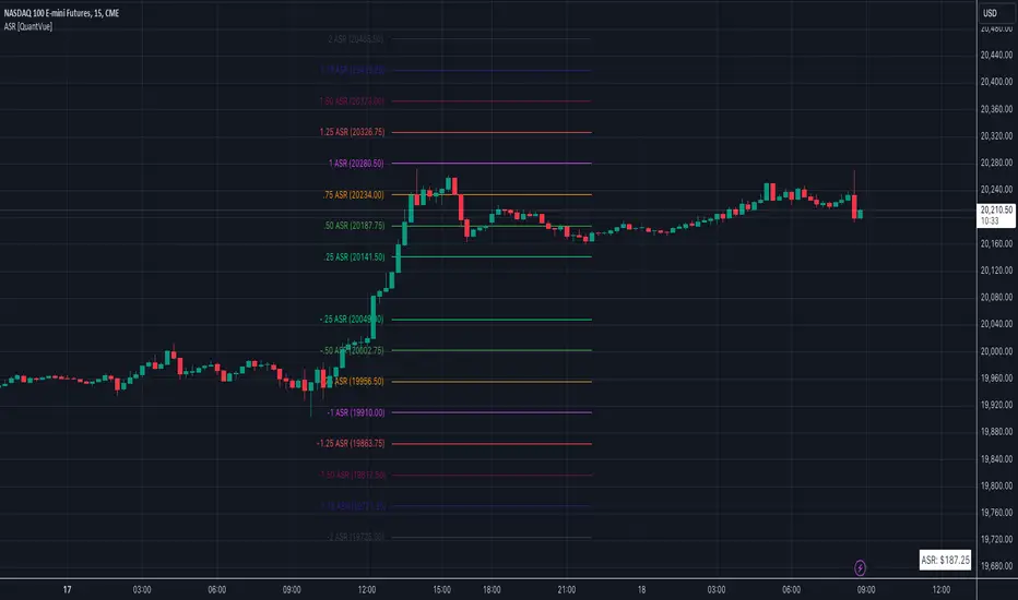
Average Session Range [QuantVue]The Average Session Range or ASR is a tool designed to find the average range of a user defined session over a user defined lookback period.
Not only is this indicator is useful for understanding volatility and price movement tendencies within sessions, but it also plots dynamic support and resistance levels based on the ASR.
The average session range is calculated over a specific period (default 14 sessions) by averaging the range (high - low) for each session.
Knowing what the ASR is allows the user to determine if current price action is normal or abnormal.
When a new session begins, potential support and resistance levels are calculated by breaking the ASR into quartiles which are then added and subtracted from the sessions opening price.
The indicator also shows an ASR label so traders can know what the ASR is in terms of dollars.
Session Time Configuration:
The indicator allows users to define the session time, with default timing set from 13:00 to 22:00.
ASR Calculation:
The ASR is calculated over a specified period (default 14 sessions) by averaging the range (high - low) of each session.
Various levels based on the ASR are computed: 0.25 ASR, 0.5 ASR, 0.75 ASR, 1 ASR, 1.25 ASR, 1.5 ASR, 1.75 ASR, and 2 ASR.
Visual Representation:
The indicator plots lines on the chart representing different ASR levels.
Customize the visibility, color, width, and style (Solid, Dashed, Dotted) of these lines for better visualization.
Labels for these lines can also be displayed, with customizable positions and text properties.
Give this indicator a BOOST and COMMENT your thoughts!
We hope you enjoy.
Cheers!
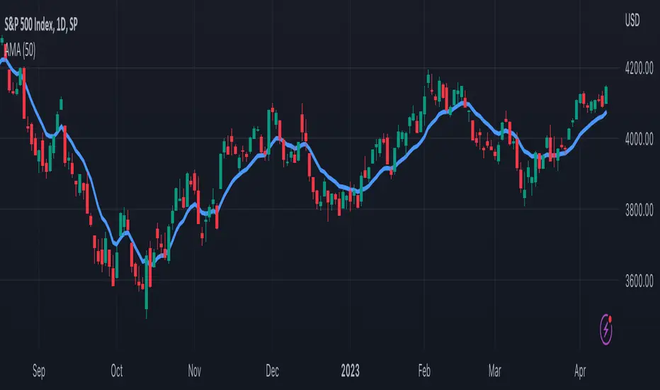
TASC 2023.05 Cong Adaptive Moving Average█ OVERVIEW
TASC's May 2023 edition of Traders' Tips features an article titled "An Adaptive Moving Average For Swing Trading" by Scott Cong. The article presents a new adaptive moving average (AMA) that adjusts its parameters automatically based on market volatility. The AMA tracks price closely during trending movements and remains flat during congestion areas.
█ CONCEPTS
Conventional moving averages (MAs) use a fixed lookback period, which may lead to limited performance in constantly changing market conditions. Perry Kaufman's adaptive moving average , first described in his 1995 book Smarter Trading, is a great example of how an AMA can self-adjust to adapt to changing environments. Scott Cong draws inspiration from Kaufman's approach and proposes a new way to calculate the AMA smoothing factor.
█ CALCULATIONS
Following Perry Kaufman's approach, Scott Cong's AMA is calculated progressively as:
AMA = α * Close + (1 − α) * AMA(1),
where:
Close = Close of the current bar
AMA(1) = AMA value of the previous bar
α = Smoothing factor between 0 and 1, defined by the lookback period
The smoothing factor determines the performance of AMA. In Cong's approach, it is calculated as:
α = Result / Effort,
where:
Result = Highest price of the n period − Lowest price of the n period
Effort = Sum(TR, n ), where TR stands for Wilder’s true range values of individual bars of the n period
n = Lookback period
As the price range is always no greater than the total journey, α is ensured to be between 0 and 1.
EMA/SMA Crossover Signals📊 EMA/SMA Crossover Signals
A professional trading indicator that identifies golden and death crosses between a customizable EMA and SMA with clear BUY/SELL labels displayed directly on your chart.
🎯 Key Features:
✅ Customizable Moving Averages - Adjust both EMA and SMA periods to match your trading strategy
✅ Clear Signal Labels - Large, color-coded "BUY" and "SELL" labels that are impossible to miss
✅ Adjustable Label Positioning - Control the vertical distance of signal labels from price action
✅ Professional Color Customization - Change colors for both moving averages and signals to match your theme
✅ Label Size Options - Choose from 4 different sizes (Tiny, Small, Normal, Large)
✅ Audio Alerts - Get notified instantly when crossovers occur
✅ Overlay Display - Signals appear directly on your price chart for better context
📈 How It Works:
🟢 BUY Signal: Triggered when the EMA crosses above the SMA (bullish crossover)
🔴 SELL Signal: Triggered when the EMA crosses below the SMA (bearish crossover)
⚙️ Customizable Settings:
Moving Averages:
- EMA Period (Default: 8)
- SMA Period (Default: 200)
Colors:
- EMA Color
- SMA Color
- Buy Signal Color
- Sell Signal Color
Signal Settings:
- Signal Vertical Offset
- Label Vertical Offset
- Label Size
💡 Best For:
- Day Trading (1-5 min timeframes)
- Swing Trading (4H-Daily)
- Trend Following Strategies
- Identifying momentum shifts
- Confirming market structure changes
🔔 Perfect for traders using ICT, Wyckoff, and institutional trading methodologies
Use this indicator as part of your complete trading system. Always combine with proper risk management and additional confluence factors.

Market Position TableMarket Position Table Indicator
Overview
The Market Position Table is a comprehensive multi-timeframe indicator that provides traders with an instant visual snapshot of market position relative to key technical indicators. This tool displays a clean, color-coded table directly on your chart, showing whether price is above or below critical moving averages, the Ichimoku Cloud, and whether the market is in a TTM Squeeze compression.
Key Features
Visual Status Dashboard
Real-time color coding: Green for bullish positioning (above), Red for bearish positioning (below/compressed)
Clean table display: Organized, easy-to-read format that doesn't clutter your chart
Customizable positioning: Place the table anywhere on your chart for optimal viewing
Technical Indicators Monitored
Four Moving Averages (20, 50, 100, 200 period)
Shows whether price is above or below each MA
Helps identify trend direction and strength
Ichimoku Cloud
Displays whether price is above, below, or inside the cloud
Gray color indicates price is within the cloud (neutral zone)
TTM Squeeze Indicator
Shows when the market is in compression (Squeeze ON = Red)
Alerts when the market is expanding (Squeeze OFF = Green)
Helps identify potential breakout opportunities
Flexible Customization
Moving Average Options:
Choose from 5 MA types: SMA, EMA, WMA, VWMA, HMA
Adjust all four MA periods to your preference
Default settings: 20, 50, 100, 200 periods
Timeframe Control:
Lock to Daily: View daily timeframe signals on any chart timeframe
Custom Timeframe: Select any specific timeframe for calculations
Chart Timeframe: Default behavior matches your current chart
Ichimoku Settings:
Customize Tenkan, Kijun, and Senkou B periods
Default: 9, 26, 52 (traditional settings)
Squeeze Settings:
Adjust Bollinger Band length and multiplier
Customize Keltner Channel length and multiplier
Fine-tune sensitivity to match your trading style
Visual Customization:
Table position: 9 placement options on your chart
Table size: Tiny, Small, Normal, or Large
Optional: Toggle MA plot lines on/off
Table Settings: Position and size
Moving Average Settings: Type and periods
Ichimoku Settings: Period adjustments
Squeeze Settings: BB and KC parameters
Timeframe Settings: Lock to daily or use custom timeframe
Interpretation
Moving Averages:
Green (ABOVE): Price is above the MA - bullish signal
Red (BELOW): Price is below the MA - bearish signal
Multiple green MAs indicate strong uptrend
Multiple red MAs indicate strong downtrend
Ichimoku Cloud:
Green (ABOVE): Price above cloud - bullish trend
Red (BELOW): Price below cloud - bearish trend
Gray (INSIDE): Price in cloud - consolidation/neutral
Squeeze Indicator:
Red (ON): Market is in compression - potential breakout setup
Green (OFF): Market is expanding - trend continuation or reversal in progress
Trading Applications
Trend Confirmation:
Use multiple green MAs + price above Ichimoku cloud to confirm strong uptrends
Use multiple red MAs + price below Ichimoku cloud to confirm strong downtrends
Breakout Trading:
Watch for Squeeze ON (red) as compression builds
When Squeeze turns OFF (green), look for directional breakout
Confirm direction with MA alignment
Multi-Timeframe Analysis:
Lock to daily timeframe while trading intraday charts
Ensure intraday trades align with daily trend direction
Example: Only take long setups on 15-min chart when daily shows green MAs
Support/Resistance:
Major MAs (50, 100, 200) often act as dynamic support/resistance
Watch for price reactions when testing these levels
Best Practices
Combine with Price Action: Use the table as confirmation alongside your chart analysis
Multi-Timeframe Confluence: Check that multiple timeframes align for higher probability setups
Don't Trade on Table Alone: Use this as one tool in your complete trading system
Customize to Your Strategy: Adjust MA types and periods to match your trading style
Monitor All Indicators: Look for alignment across all indicators for strongest signals
Tips for Optimal Use
Day Traders: Enable "Lock to Daily" to stay aligned with the daily trend while trading shorter timeframes
Swing Traders: Use default chart timeframe on daily or weekly charts
Trend Followers: Focus on MA alignment - all green or all red indicates strong trends
Breakout Traders: Watch the Squeeze indicator closely for compression/expansion cycles
Position Traders: Use longer MA periods (e.g., 50, 100, 150, 200) for smoother signals

HTF BIAS FILTER🧭HTF Bias Filter Indicator: 5 in 1 indicator
Technical Overview
The Bias Filter is a comprehensive multi-timeframe tool designed to confirm directional bias using five key indicators before entering a trade. It plots higher-timeframe Moving Averages directly on the chart and provides an immediate status summary via a static dashboard.
The more confluence on the dashboard, the greater the probability of the direction of the trade.
1. 📊 Display Components
A. Plotted Lines
The indicator uses the request.security function to draw Moving Averages from higher timeframes onto your current chart:
1H EMA 21 (Purple): The 21-period Exponential Moving Average calculated on the 1-Hour (60 min) chart. Plotted using a step-line style.
4H EMA 50 (Red): The 50-period Exponential Moving Average calculated on the 4-Hour (240 min) chart. Plotted using a step-line style.
B. Directional Dashboard
A fixed-position summary table is anchored to the bottom-right corner of the chart, providing a quick glance at the current status of all five filters.
2. 🎨 Colour Logic
Each of the five indicators is assigned a colour based on its current directional signal. The more indicators that show the same colour (confluence), the stronger the signal and the higher the likelihood of a high-probability trade.
🟢 Green indicators are signaling UP/BUY (Bullish momentum or trend).
🔴 Red indicators are signaling DOWN/SELL (Bearish momentum or trend).
⚫ Gray indicators are signaling Mixed or flat directions (neutral or undecided).
Note: The dashboard's main header color is determined by a strict confluence logic (All four 4H filters must align for Green/Red), while individual indicator colors follow the simple rules above.
3. 📋 Indicator Breakdown and Logic
The dashboard provides the direction of five different filters.
3.1. Higher-Timeframe (HTF) Trend Indicators
These two signals determine the immediate slope and direction of the primary Moving Averages:
4H EMA 50:
Timeframe: 4-Hour (240 min)
Logic: Compares the current EMA value to the value two bars ago on the 4H chart.
Output: UP ↑, DOWN ↓, or FLAT ⏸
1H EMA 21:
Timeframe: 1-Hour (60 min)
Logic: Compares the current EMA value to the value two bars ago on the 1H chart.
Output: UP ↑, DOWN ↓, or FLAT ⏸
3.2. 4-Hour Confluence Filters
These three indicators provide supplementary confirmation on Volume, Price Position, and Momentum, all calculated on the 4-Hour (240 min) chart:
4H OBV (Smoothed):
Timeframe: 4-Hour (240 min)
Logic: Direction is based on the current value of the 21-bar smoothed On-Balance Volume (OBV) compared to its value nine bars ago.
Output: UP ↑, DOWN ↓, or FLAT ⏸
4H ATR DIR (EMA Proxy):
Timeframe: 4-Hour (240 min)
Logic: Determines the price position by comparing the current Close price against the 4H EMA 50.
Output: BUY 🟢 (Close > EMA 50), SELL 🔴 (Close < EMA 50), or FLAT ⏸️ (Close = EMA 50).
4H RSI (14):
Timeframe: 4-Hour (240 min)
Logic: Momentum check comparing the 14-period Relative Strength Index (RSI) value against the 50 level.
Output: BUY 🟢 (RSI > 50), SELL 🔴 (RSI < 50), or FLAT ⏸️ (RSI = 50).

Moving Aaverage (EMA) & VWAP by Vish
Multi-Timeframe Moving Averages with VWAP
This indicator combines essential moving averages with VWAP to provide comprehensive trend analysis on a single chart. Designed for traders who need quick visual reference of multiple timeframes and volume-weighted price levels.
Features:
• Six customizable moving averages: 8, 13, 21, 50, 100, and 200 periods
• Toggle between Simple Moving Average (SMA) and Exponential Moving Average (EMA) for all lines
• Individual on/off controls for each moving average
• Volume Weighted Average Price (VWAP) with customizable settings
• VWAP anchor options: Session, Week, Month, Quarter, and Year
• Clean, color-coded visualization for easy identification
• Fully customizable through settings panel
Use Cases:
• Identify trend direction across multiple timeframes
• Find dynamic support and resistance levels
• Spot potential entry and exit points
• Analyze price action relative to volume-weighted average
• Confirm trend strength with multiple MA convergence/divergence
Settings:
All parameters are adjustable including MA type (SMA/EMA), individual MA visibility, VWAP source, and VWAP anchor period.
Suitable for all markets and timeframes. Works on stocks, forex, crypto, commodities, and indices.
#moving average #MA #EMA #SMA #VWAP #trend #support #resistance #multi-timeframe

LibWghtLibrary "LibWght"
This is a library of mathematical and statistical functions
designed for quantitative analysis in Pine Script. Its core
principle is the integration of a custom weighting series
(e.g., volume) into a wide array of standard technical
analysis calculations.
Key Capabilities:
1. **Universal Weighting:** All exported functions accept a `weight`
parameter. This allows standard calculations (like moving
averages, RSI, and standard deviation) to be influenced by an
external data series, such as volume or tick count.
2. **Weighted Averages and Indicators:** Includes a comprehensive
collection of weighted functions:
- **Moving Averages:** `wSma`, `wEma`, `wWma`, `wRma` (Wilder's),
`wHma` (Hull), and `wLSma` (Least Squares / Linear Regression).
- **Oscillators & Ranges:** `wRsi`, `wAtr` (Average True Range),
`wTr` (True Range), and `wR` (High-Low Range).
3. **Volatility Decomposition:** Provides functions to decompose
total variance into distinct components for market analysis.
- **Two-Way Decomposition (`wTotVar`):** Separates variance into
**between-bar** (directional) and **within-bar** (noise)
components.
- **Three-Way Decomposition (`wLRTotVar`):** Decomposes variance
relative to a linear regression into **Trend** (explained by
the LR slope), **Residual** (mean-reversion around the
LR line), and **Within-Bar** (noise) components.
- **Local Volatility (`wLRLocTotStdDev`):** Measures the total
"noise" (within-bar + residual) around the trend line.
4. **Weighted Statistics and Regression:** Provides a robust
function for Weighted Linear Regression (`wLinReg`) and a
full suite of related statistical measures:
- **Between-Bar Stats:** `wBtwVar`, `wBtwStdDev`, `wBtwStdErr`.
- **Residual Stats:** `wResVar`, `wResStdDev`, `wResStdErr`.
5. **Fallback Mechanism:** All functions are designed for reliability.
If the total weight over the lookback period is zero (e.g., in
a no-volume period), the algorithms automatically fall back to
their unweighted, uniform-weight equivalents (e.g., `wSma`
becomes a standard `ta.sma`), preventing errors and ensuring
continuous calculation.
---
**DISCLAIMER**
This library is provided "AS IS" and for informational and
educational purposes only. It does not constitute financial,
investment, or trading advice.
The author assumes no liability for any errors, inaccuracies,
or omissions in the code. Using this library to build
trading indicators or strategies is entirely at your own risk.
As a developer using this library, you are solely responsible
for the rigorous testing, validation, and performance of any
scripts you create based on these functions. The author shall
not be held liable for any financial losses incurred directly
or indirectly from the use of this library or any scripts
derived from it.
wSma(source, weight, length)
Weighted Simple Moving Average (linear kernel).
Parameters:
source (float) : series float Data to average.
weight (float) : series float Weight series.
length (int) : series int Look-back length ≥ 1.
Returns: series float Linear-kernel weighted mean; falls back to
the arithmetic mean if Σweight = 0.
wEma(source, weight, length)
Weighted EMA (exponential kernel).
Parameters:
source (float) : series float Data to average.
weight (float) : series float Weight series.
length (simple int) : simple int Look-back length ≥ 1.
Returns: series float Exponential-kernel weighted mean; falls
back to classic EMA if Σweight = 0.
wWma(source, weight, length)
Weighted WMA (linear kernel).
Parameters:
source (float) : series float Data to average.
weight (float) : series float Weight series.
length (int) : series int Look-back length ≥ 1.
Returns: series float Linear-kernel weighted mean; falls back to
classic WMA if Σweight = 0.
wRma(source, weight, length)
Weighted RMA (Wilder kernel, α = 1/len).
Parameters:
source (float) : series float Data to average.
weight (float) : series float Weight series.
length (simple int) : simple int Look-back length ≥ 1.
Returns: series float Wilder-kernel weighted mean; falls back to
classic RMA if Σweight = 0.
wHma(source, weight, length)
Weighted HMA (linear kernel).
Parameters:
source (float) : series float Data to average.
weight (float) : series float Weight series.
length (int) : series int Look-back length ≥ 1.
Returns: series float Linear-kernel weighted mean; falls back to
classic HMA if Σweight = 0.
wRsi(source, weight, length)
Weighted Relative Strength Index.
Parameters:
source (float) : series float Price series.
weight (float) : series float Weight series.
length (simple int) : simple int Look-back length ≥ 1.
Returns: series float Weighted RSI; uniform if Σw = 0.
wAtr(tr, weight, length)
Weighted ATR (Average True Range).
Implemented as WRMA on *true range*.
Parameters:
tr (float) : series float True Range series.
weight (float) : series float Weight series.
length (simple int) : simple int Look-back length ≥ 1.
Returns: series float Weighted ATR; uniform weights if Σw = 0.
wTr(tr, weight, length)
Weighted True Range over a window.
Parameters:
tr (float) : series float True Range series.
weight (float) : series float Weight series.
length (int) : series int Look-back length ≥ 1.
Returns: series float Weighted mean of TR; uniform if Σw = 0.
wR(r, weight, length)
Weighted High-Low Range over a window.
Parameters:
r (float) : series float High-Low per bar.
weight (float) : series float Weight series.
length (int) : series int Look-back length ≥ 1.
Returns: series float Weighted mean of range; uniform if Σw = 0.
wBtwVar(source, weight, length, biased)
Weighted Between Variance (biased/unbiased).
Parameters:
source (float) : series float Data series.
weight (float) : series float Weight series.
length (int) : series int Look-back length ≥ 2.
biased (bool) : series bool true → population (biased); false → sample.
Returns:
variance series float The calculated between-bar variance (σ²btw), either biased or unbiased.
sumW series float The sum of weights over the lookback period (Σw).
sumW2 series float The sum of squared weights over the lookback period (Σw²).
wBtwStdDev(source, weight, length, biased)
Weighted Between Standard Deviation.
Parameters:
source (float) : series float Data series.
weight (float) : series float Weight series.
length (int) : series int Look-back length ≥ 2.
biased (bool) : series bool true → population (biased); false → sample.
Returns: series float σbtw uniform if Σw = 0.
wBtwStdErr(source, weight, length, biased)
Weighted Between Standard Error.
Parameters:
source (float) : series float Data series.
weight (float) : series float Weight series.
length (int) : series int Look-back length ≥ 2.
biased (bool) : series bool true → population (biased); false → sample.
Returns: series float √(σ²btw / N_eff) uniform if Σw = 0.
wTotVar(mu, sigma, weight, length, biased)
Weighted Total Variance (= between-group + within-group).
Useful when each bar represents an aggregate with its own
mean* and pre-estimated σ (e.g., second-level ranges inside a
1-minute bar). Assumes the *weight* series applies to both the
group means and their σ estimates.
Parameters:
mu (float) : series float Group means (e.g., HL2 of 1-second bars).
sigma (float) : series float Pre-estimated σ of each group (same basis).
weight (float) : series float Weight series (volume, ticks, …).
length (int) : series int Look-back length ≥ 2.
biased (bool) : series bool true → population (biased); false → sample.
Returns:
varBtw series float The between-bar variance component (σ²btw).
varWtn series float The within-bar variance component (σ²wtn).
sumW series float The sum of weights over the lookback period (Σw).
sumW2 series float The sum of squared weights over the lookback period (Σw²).
wTotStdDev(mu, sigma, weight, length, biased)
Weighted Total Standard Deviation.
Parameters:
mu (float) : series float Group means (e.g., HL2 of 1-second bars).
sigma (float) : series float Pre-estimated σ of each group (same basis).
weight (float) : series float Weight series (volume, ticks, …).
length (int) : series int Look-back length ≥ 2.
biased (bool) : series bool true → population (biased); false → sample.
Returns: series float σtot.
wTotStdErr(mu, sigma, weight, length, biased)
Weighted Total Standard Error.
SE = √( total variance / N_eff ) with the same effective sample
size logic as `wster()`.
Parameters:
mu (float) : series float Group means (e.g., HL2 of 1-second bars).
sigma (float) : series float Pre-estimated σ of each group (same basis).
weight (float) : series float Weight series (volume, ticks, …).
length (int) : series int Look-back length ≥ 2.
biased (bool) : series bool true → population (biased); false → sample.
Returns: series float √(σ²tot / N_eff).
wLinReg(source, weight, length)
Weighted Linear Regression.
Parameters:
source (float) : series float Data series.
weight (float) : series float Weight series.
length (int) : series int Look-back length ≥ 2.
Returns:
mid series float The estimated value of the regression line at the most recent bar.
slope series float The slope of the regression line.
intercept series float The intercept of the regression line.
wResVar(source, weight, midLine, slope, length, biased)
Weighted Residual Variance.
linear regression – optionally biased (population) or
unbiased (sample).
Parameters:
source (float) : series float Data series.
weight (float) : series float Weighting series (volume, etc.).
midLine (float) : series float Regression value at the last bar.
slope (float) : series float Slope per bar.
length (int) : series int Look-back length ≥ 2.
biased (bool) : series bool true → population variance (σ²_P), denominator ≈ N_eff.
false → sample variance (σ²_S), denominator ≈ N_eff - 2.
(Adjusts for 2 degrees of freedom lost to the regression).
Returns:
variance series float The calculated residual variance (σ²res), either biased or unbiased.
sumW series float The sum of weights over the lookback period (Σw).
sumW2 series float The sum of squared weights over the lookback period (Σw²).
wResStdDev(source, weight, midLine, slope, length, biased)
Weighted Residual Standard Deviation.
Parameters:
source (float) : series float Data series.
weight (float) : series float Weight series.
midLine (float) : series float Regression value at the last bar.
slope (float) : series float Slope per bar.
length (int) : series int Look-back length ≥ 2.
biased (bool) : series bool true → population (biased); false → sample.
Returns: series float σres; uniform if Σw = 0.
wResStdErr(source, weight, midLine, slope, length, biased)
Weighted Residual Standard Error.
Parameters:
source (float) : series float Data series.
weight (float) : series float Weight series.
midLine (float) : series float Regression value at the last bar.
slope (float) : series float Slope per bar.
length (int) : series int Look-back length ≥ 2.
biased (bool) : series bool true → population (biased); false → sample.
Returns: series float √(σ²res / N_eff); uniform if Σw = 0.
wLRTotVar(mu, sigma, weight, midLine, slope, length, biased)
Weighted Linear-Regression Total Variance **around the
window’s weighted mean μ**.
σ²_tot = E_w ⟶ *within-group variance*
+ Var_w ⟶ *residual variance*
+ Var_w ⟶ *trend variance*
where each bar i in the look-back window contributes
m_i = *mean* (e.g. 1-sec HL2)
σ_i = *sigma* (pre-estimated intrabar σ)
w_i = *weight* (volume, ticks, …)
ŷ_i = b₀ + b₁·x (value of the weighted LR line)
r_i = m_i − ŷ_i (orthogonal residual)
Parameters:
mu (float) : series float Per-bar mean m_i.
sigma (float) : series float Pre-estimated σ_i of each bar.
weight (float) : series float Weight series w_i (≥ 0).
midLine (float) : series float Regression value at the latest bar (ŷₙ₋₁).
slope (float) : series float Slope b₁ of the regression line.
length (int) : series int Look-back length ≥ 2.
biased (bool) : series bool true → population; false → sample.
Returns:
varRes series float The residual variance component (σ²res).
varWtn series float The within-bar variance component (σ²wtn).
varTrd series float The trend variance component (σ²trd), explained by the linear regression.
sumW series float The sum of weights over the lookback period (Σw).
sumW2 series float The sum of squared weights over the lookback period (Σw²).
wLRTotStdDev(mu, sigma, weight, midLine, slope, length, biased)
Weighted Linear-Regression Total Standard Deviation.
Parameters:
mu (float) : series float Per-bar mean m_i.
sigma (float) : series float Pre-estimated σ_i of each bar.
weight (float) : series float Weight series w_i (≥ 0).
midLine (float) : series float Regression value at the latest bar (ŷₙ₋₁).
slope (float) : series float Slope b₁ of the regression line.
length (int) : series int Look-back length ≥ 2.
biased (bool) : series bool true → population; false → sample.
Returns: series float √(σ²tot).
wLRTotStdErr(mu, sigma, weight, midLine, slope, length, biased)
Weighted Linear-Regression Total Standard Error.
SE = √( σ²_tot / N_eff ) with N_eff = Σw² / Σw² (like in wster()).
Parameters:
mu (float) : series float Per-bar mean m_i.
sigma (float) : series float Pre-estimated σ_i of each bar.
weight (float) : series float Weight series w_i (≥ 0).
midLine (float) : series float Regression value at the latest bar (ŷₙ₋₁).
slope (float) : series float Slope b₁ of the regression line.
length (int) : series int Look-back length ≥ 2.
biased (bool) : series bool true → population; false → sample.
Returns: series float √((σ²res, σ²wtn, σ²trd) / N_eff).
wLRLocTotStdDev(mu, sigma, weight, midLine, slope, length, biased)
Weighted Linear-Regression Local Total Standard Deviation.
Measures the total "noise" (within-bar + residual) around the trend.
Parameters:
mu (float) : series float Per-bar mean m_i.
sigma (float) : series float Pre-estimated σ_i of each bar.
weight (float) : series float Weight series w_i (≥ 0).
midLine (float) : series float Regression value at the latest bar (ŷₙ₋₁).
slope (float) : series float Slope b₁ of the regression line.
length (int) : series int Look-back length ≥ 2.
biased (bool) : series bool true → population; false → sample.
Returns: series float √(σ²wtn + σ²res).
wLRLocTotStdErr(mu, sigma, weight, midLine, slope, length, biased)
Weighted Linear-Regression Local Total Standard Error.
Parameters:
mu (float) : series float Per-bar mean m_i.
sigma (float) : series float Pre-estimated σ_i of each bar.
weight (float) : series float Weight series w_i (≥ 0).
midLine (float) : series float Regression value at the latest bar (ŷₙ₋₁).
slope (float) : series float Slope b₁ of the regression line.
length (int) : series int Look-back length ≥ 2.
biased (bool) : series bool true → population; false → sample.
Returns: series float √((σ²wtn + σ²res) / N_eff).
wLSma(source, weight, length)
Weighted Least Square Moving Average.
Parameters:
source (float) : series float Data series.
weight (float) : series float Weight series.
length (int) : series int Look-back length ≥ 2.
Returns: series float Least square weighted mean. Falls back
to unweighted regression if Σw = 0.
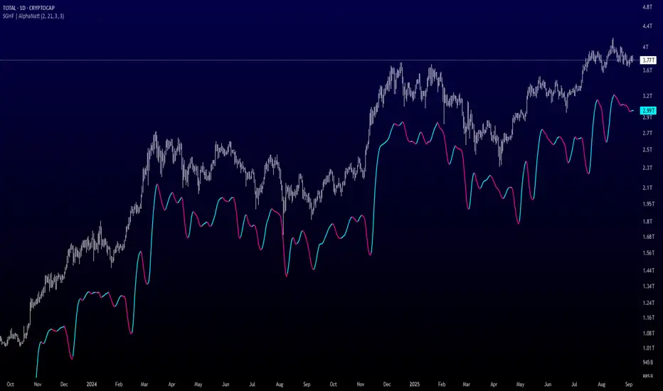
Arnaud Legoux Gaussian Flow | AlphaNattArnaud Legoux Gaussian Flow | AlphaNatt
A sophisticated trend-following and mean-reversion indicator that combines the power of the Arnaud Legoux Moving Average (ALMA) with advanced Gaussian distribution analysis to identify high-probability trading opportunities.
🎯 What Makes This Indicator Unique?
This indicator goes beyond traditional moving averages by incorporating Gaussian mathematics at multiple levels:
ALMA uses Gaussian distribution for superior price smoothing with minimal lag
Dynamic envelopes based on Gaussian probability zones
Multi-layer gradient visualization showing probability density
Adaptive envelope modes that respond to market conditions
📊 Core Components
1. Arnaud Legoux Moving Average (ALMA)
The ALMA is a highly responsive moving average that uses Gaussian distribution to weight price data. Unlike simple moving averages, ALMA can be fine-tuned to balance responsiveness and smoothness through three key parameters:
ALMA Period: Controls the lookback window (default: 21)
Gaussian Offset: Shifts the Gaussian curve to adjust lag vs. responsiveness (default: 0.85)
Gaussian Sigma: Controls the width of the Gaussian distribution (default: 6.0)
2. Gaussian Envelope System
The indicator features three envelope calculation modes:
Fixed Mode: Uses ATR-based fixed width for consistent envelope sizing
Adaptive Mode: Dynamically adjusts based on price acceleration and volatility
Hybrid Mode: Combines ATR and standard deviation for balanced adaptation
The envelopes represent statistical probability zones. Price moving beyond these zones suggests potential mean reversion opportunities.
3. Momentum-Adjusted Envelopes
The envelope width automatically expands during strong trends and contracts during consolidation, providing context-aware support and resistance levels.
⚡ Key Features
Multi-Layer Gradient Visualization
The indicator displays 10 gradient layers between the ALMA and envelope boundaries, creating a visual "heat map" of probability density. This helps traders quickly assess:
Distance from the mean
Potential support/resistance strength
Overbought/oversold conditions in context
Dynamic Color Coding
Cyan gradient: Price below ALMA (bullish zone)
Magenta gradient: Price above ALMA (bearish zone)
The ALMA line itself changes color based on price position
Trend Regime Detection
The indicator automatically identifies market regimes:
Strong Uptrend: Trend strength > 0.5% with price above ALMA
Strong Downtrend: Trend strength < -0.5% with price below ALMA
Weak trends and ranging conditions
📈 Trading Strategies
Mean Reversion Strategy
Look for price entering the extreme Gaussian zones (beyond 95% of envelope width) when trend strength is moderate. These represent statistical extremes where mean reversion is probable.
Signals:
Long: Price in lower Gaussian zone with trend strength > -0.5%
Short: Price in upper Gaussian zone with trend strength < 0.5%
Trend Continuation Strategy
Enter when price crosses the ALMA during confirmed strong trend conditions, riding momentum while using the envelope as a trailing stop reference.
Signals:
Long: Price crosses above ALMA during strong uptrend
Short: Price crosses below ALMA during strong downtrend
🎨 Visualization Guide
The gradient layers create a "probability cloud" around the ALMA:
Darker shades (near ALMA): High probability zone - price tends to stay here
Lighter shades (near envelope edges): Lower probability - potential reversal zones
Price at envelope extremes: Statistical outliers - strongest mean reversion setups
⚙️ Customization Options
ALMA Parameters
Adjust period for different timeframes (lower for day trading, higher for swing trading)
Modify offset to tune responsiveness vs. smoothness
Change sigma to control distribution width
Envelope Configuration
Choose envelope mode based on market characteristics
Adjust multiplier to match instrument volatility
Modify gradient depth for visual preference (5-15 layers)
Signal Enhancement
Momentum Length: Lookback for trend strength calculation
Signal Smoothing: Additional EMA smoothing to reduce noise
🔔 Built-in Alerts
The indicator includes six pre-configured alert conditions:
ALMA Trend Long - Price crosses above ALMA in strong uptrend
ALMA Trend Short - Price crosses below ALMA in strong downtrend
Mean Reversion Long - Price enters lower Gaussian zone
Mean Reversion Short - Price enters upper Gaussian zone
Strong Uptrend Detected - Momentum confirms strong bullish regime
Strong Downtrend Detected - Momentum confirms strong bearish regime
💡 Best Practices
Use on clean, liquid markets with consistent volatility
Combine with volume analysis for confirmation
Adjust envelope multiplier based on backtesting for your specific instrument
Higher timeframes (4H+) generally provide more reliable signals
Use adaptive mode for trending markets, hybrid for mixed conditions
⚠️ Important Notes
This indicator works best in markets with normal price distribution
Extreme news events can invalidate Gaussian assumptions temporarily
Always use proper risk management - no indicator is perfect
Backtest parameters on your specific instrument and timeframe
🔬 Technical Background
The Arnaud Legoux Moving Average was developed to solve the classic dilemma of moving averages: the trade-off between lag and noise. By applying Gaussian distribution weighting, ALMA achieves superior smoothing while maintaining responsiveness to price changes.
The envelope system extends this concept by creating probability zones based on volatility and momentum, effectively mapping where price is "likely" vs "unlikely" to be found based on statistical principles.
Created by AlphaNatt - For educational purposes. Always practice proper risk management. Not financial advice. Always DYOR.

Savitzky-Golay Hampel Filter | AlphaNattSavitzky-Golay Hampel Filter | AlphaNatt
A revolutionary indicator combining NASA's satellite data processing algorithms with robust statistical outlier detection to create the most scientifically advanced trend filter available on TradingView.
"This is the same mathematics that processes signals from the Hubble Space Telescope and analyzes data from the Large Hadron Collider - now applied to financial markets."
━━━━━━━━━━━━━━━━━━━━━━━━━━━━━━━━━━━━━━━━
🚀 SCIENTIFIC PEDIGREE
Savitzky-Golay Filter Applications:
NASA: Satellite telemetry and space probe data processing
CERN: Particle physics data analysis at the LHC
Pharmaceutical: Chromatography and spectroscopy analysis
Astronomy: Processing signals from radio telescopes
Medical: ECG and EEG signal processing
Hampel Filter Usage:
Aerospace: Cleaning sensor data from aircraft and spacecraft
Manufacturing: Quality control in precision engineering
Seismology: Earthquake detection and analysis
Robotics: Sensor fusion and noise reduction
━━━━━━━━━━━━━━━━━━━━━━━━━━━━━━━━━━━━━━━━
🧬 THE MATHEMATICS
1. Savitzky-Golay Filter
The SG filter performs local polynomial regression on data points:
Fits a polynomial of degree n to a sliding window of data
Evaluates the polynomial at the center point
Preserves higher moments (peaks, valleys) unlike moving averages
Maintains derivative information for true momentum analysis
Originally published in Analytical Chemistry (1964)
Mathematical Properties:
Optimal smoothing in the least-squares sense
Preserves statistical moments up to polynomial order
Exact derivative calculation without additional lag
Superior frequency response vs traditional filters
2. Hampel Filter
A robust outlier detector based on Median Absolute Deviation (MAD):
Identifies outliers using robust statistics
Replaces spurious values with polynomial-fitted estimates
Resistant to up to 50% contaminated data
MAD is 1.4826 times more robust than standard deviation
Outlier Detection Formula:
|x - median| > k × 1.4826 × MAD
Where k is the threshold parameter (typically 3 for 99.7% confidence)
━━━━━━━━━━━━━━━━━━━━━━━━━━━━━━━━━━━━━━━━
💎 WHY THIS IS SUPERIOR
vs Moving Averages:
Preserves peaks and valleys (critical for catching tops/bottoms)
No lag penalty for smoothness
Maintains derivative information
Polynomial fitting > simple averaging
vs Other Filters:
Outlier immunity (Hampel component)
Scientifically optimal smoothing
Preserves higher-order features
Used in billion-dollar research projects
Unique Advantages:
Feature Preservation: Maintains market structure while smoothing
Spike Immunity: Ignores false breakouts and stop hunts
Derivative Accuracy: True momentum without additional indicators
Scientific Validation: 60+ years of academic research
━━━━━━━━━━━━━━━━━━━━━━━━━━━━━━━━━━━━━━━━
⚙️ PARAMETER OPTIMIZATION
1. Polynomial Order (2-5)
2 (Quadratic): Maximum smoothing, gentle curves
3 (Cubic): Balanced smoothing and responsiveness (recommended)
4-5 (Higher): More responsive, preserves more features
2. Window Size (7-51)
Must be odd number
Larger = smoother but more lag
Formula: 2×(desired smoothing period) + 1
Default 21 = analyzes 10 bars each side
3. Hampel Threshold (1.0-5.0)
1.0: Aggressive outlier removal (68% confidence)
2.0: Moderate outlier removal (95% confidence)
3.0: Conservative outlier removal (99.7% confidence) (default)
4.0+: Only extreme outliers removed
4. Final Smoothing (1-7)
Additional WMA smoothing after filtering
1 = No additional smoothing
3-5 = Recommended for most timeframes
7 = Ultra-smooth for position trading
━━━━━━━━━━━━━━━━━━━━━━━━━━━━━━━━━━━━━━━━
📊 TRADING STRATEGIES
Signal Recognition:
Cyan Line: Bullish trend with positive derivative
Pink Line: Bearish trend with negative derivative
Color Change: Trend reversal with polynomial confirmation
1. Trend Following Strategy
Enter when price crosses above cyan filter
Exit when filter turns pink
Use filter as dynamic stop loss
Best in trending markets
2. Mean Reversion Strategy
Enter long when price touches filter from below in uptrend
Enter short when price touches filter from above in downtrend
Exit at opposite band or filter color change
Excellent for range-bound markets
3. Derivative Strategy (Advanced)
The SG filter preserves derivative information
Acceleration = second derivative > 0
Enter on positive first derivative + positive acceleration
Exit on negative second derivative (momentum slowing)
━━━━━━━━━━━━━━━━━━━━━━━━━━━━━━━━━━━━━━━━
📈 PERFORMANCE CHARACTERISTICS
Strengths:
Outlier Immunity: Ignores stop hunts and flash crashes
Feature Preservation: Catches tops/bottoms better than MAs
Smooth Output: Reduces whipsaws significantly
Scientific Basis: Not curve-fitted or optimized to markets
Considerations:
Slight lag in extreme volatility (all filters have this)
Requires odd window sizes (mathematical requirement)
More complex than simple moving averages
Best with liquid instruments
━━━━━━━━━━━━━━━━━━━━━━━━━━━━━━━━━━━━━━━━
🔬 SCIENTIFIC BACKGROUND
Savitzky-Golay Publication:
"Smoothing and Differentiation of Data by Simplified Least Squares Procedures"
- Abraham Savitzky & Marcel Golay
- Analytical Chemistry, Vol. 36, No. 8, 1964
Hampel Filter Origin:
"Robust Statistics: The Approach Based on Influence Functions"
- Frank Hampel et al., 1986
- Princeton University Press
These techniques have been validated in thousands of scientific papers and are standard tools in:
NASA's Jet Propulsion Laboratory
European Space Agency
CERN (Large Hadron Collider)
MIT Lincoln Laboratory
Max Planck Institutes
━━━━━━━━━━━━━━━━━━━━━━━━━━━━━━━━━━━━━━━━
💡 ADVANCED TIPS
News Trading: Lower Hampel threshold before major events to catch spikes
Scalping: Use Order=2 for maximum smoothness, Window=11 for responsiveness
Position Trading: Increase Window to 31+ for long-term trends
Combine with Volume: Strong trends need volume confirmation
Multiple Timeframes: Use daily for trend, hourly for entry
Watch the Derivative: Filter color changes when first derivative changes sign
━━━━━━━━━━━━━━━━━━━━━━━━━━━━━━━━━━━━━━━━
⚠️ IMPORTANT NOTICES
Not financial advice - educational purposes only
Past performance does not guarantee future results
Always use proper risk management
Test settings on your specific instrument and timeframe
No indicator is perfect - part of complete trading system
━━━━━━━━━━━━━━━━━━━━━━━━━━━━━━━━━━━━━━━━
🏆 CONCLUSION
The Savitzky-Golay Hampel Filter represents the pinnacle of scientific signal processing applied to financial markets. By combining polynomial regression with robust outlier detection, traders gain access to the same mathematical tools that:
Guide spacecraft to other planets
Detect gravitational waves from black holes
Analyze particle collisions at near light-speed
Process signals from deep space
This isn't just another indicator - it's rocket science for trading .
"When NASA needs to separate signal from noise in billion-dollar missions, they use these exact algorithms. Now you can too."
━━━━━━━━━━━━━━━━━━━━━━━━━━━━━━━━━━━━━━━━
Developed by AlphaNatt
Version: 1.0
Release: 2025
Pine Script: v6
"Where Space Technology Meets Market Analysis"
Not financial advice. Always DYOR
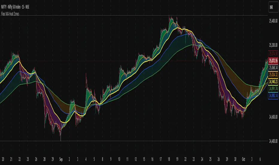
Flexi MA Heat ZonesOverview
Flexi MA Heat Zones is a powerful multi-timeframe visualization tool that helps traders easily identify trend strength, direction, and potential zones of confluence using multiple moving averages and dynamic heatmaps. The indicator plots up to three pairs of customizable moving averages, with color-coded heat zones to highlight bullish and bearish conditions at a glance.
Whether you're a trend follower, mean-reversion trader, or looking for visual confirmation zones, this indicator is designed to offer deep insights with high customizability.
⚙️ Key Features
🔄 Supports multiple MA types: Choose from EMA, SMA, WMA, VWMA to suit your strategy.
🎯 Six moving averages: Three MA pairs (MA1-MA2, MA3-MA4, MA5-MA6), each with independent lengths and colors.
🌈 Heatmap Zones: Dynamic fills between MA pairs, changing color based on bullish or bearish alignment.
👁️🗨️ Full customization: Enable/disable any MA pair and its heatmap zone from the settings.
🪞 Transparency controls: Adjust the visibility of heat zones for clarity or stylistic preference.
🎨 Color-coded for clarity: Bullish and bearish colors for each heat zone pair, fully user-configurable.
🧩 Efficient layout: Smart use of grouped inputs for easier configuration and visibility management.
📈 How to Use
Use the MA1–MA2 and MA3–MA4 zones for longer-term trend tracking and confluence analysis.
Use the faster MA5–MA6 zone for short-term micro-trend identification or scalping.
When a faster MA is above the slower one within a pair, the fill turns bullish (user-defined color).
When the faster MA is below the slower one, the fill turns bearish.
Combine with price action or other indicators for entry/exit confirmation.
🧠 Pro Tips
For trend-following strategies, consider using EMA or WMA types.
For mean-reversion or support/resistance zones, SMA and VWMA may offer better zone clarity.
Overlay with RSI, MACD, or custom entry signals for higher confidence setups.
Use different heatmap transparencies to visually separate overlapping MA zones.
THF Crossover and Trend Signals Golden & Death Cross with VolumeScript Overview:
This Pine Script is designed to assist traders in identifying key buy/sell signals and major trend changes on the chart using Exponential Moving Averages (EMA) and Simple Moving Averages (SMA), as well as visualizing Golden Cross and Death Cross events. The script also includes a volume indicator to highlight the volume trading activity in relation to the price movements.
Key Features:
1. Moving Averages:
EMA 21: Exponential Moving Average over a 21-period, shown in green.
EMA 50: Exponential Moving Average over a 50-period, shown in yellow.
SMA 50: Simple Moving Average over a 50-period, shown in red.
SMA 200: Simple Moving Average over a 200-period, shown in blue.
2. Signals:
Buy Signal: Generated when EMA 21 crosses above SMA 50, indicating a potential upward trend. Displayed with a green label below the price bar.
Sell Signal: Generated when EMA 21 crosses below SMA 50, indicating a potential downward trend. Displayed with a red label above the price bar.
3. Golden Cross (Bullish Trend):
A Golden Cross occurs when EMA 50 crosses above SMA 200, which often signals the start of a long-term upward trend. The signal is displayed with a yellow label below the price bar.
4. Death Cross (Bearish Trend):
A Death Cross occurs when EMA 50 crosses below SMA 200, which often signals the start of a long-term downward trend. The signal is displayed with a blue label above the price bar.
5. Volume Indicator:
The volume is plotted as colored columns. Green indicates higher volume than the 20-period moving average, and red indicates lower volume.
A Volume Moving Average (SMA 20) is also plotted to compare volume changes over time.
How the Script Works:
1. The EMA and SMA lines are plotted on the chart, providing a visual representation of the short- and long-term trends.
2. Buy/Sell signals are triggered based on the crossover between EMA 21 and SMA 50, helping to identify potential entry and exit points.
3. The Golden Cross and Death Cross indicators highlight major trend reversals based on the crossover between EMA 50 and SMA 200, providing clear visual cues for long-term trend changes.
4. Volume is displayed alongside price movements, offering insight into the strength or weakness of a trend.
Key Customizations:
Moving Average Periods: Users can modify the lengths of the EMAs and SMAs for customized analysis.
Volume Moving Average Period: The script allows for adjustment of the volume moving average period to suit different market conditions.
Signal Visibility: The size and color of the buy, sell, Golden Cross, and Death Cross signals can be easily customized to make them more prominent on the chart.
Conclusion:
This script is ideal for traders looking to combine price action with volume analysis, using key technical indicators such as EMA, SMA, Golden Cross, and Death Cross to make informed decisions in trending markets.
---
This explanation covers all aspects of the script and provides a clear understanding of its functionality, which is helpful for sharing the script or using it as an educational resource.

Uptrick: Fusion Trend Reversion SystemOverview
The Uptrick: Fusion Trend Reversion System is a multi-layered indicator designed to identify potential price reversals during intraday movement while keeping traders informed of the dominant short-term trend. It blends a composite fair value model with deviation logic and a refined momentum filter using the Relative Strength Index (RSI). This tool was created with scalpers and short-term traders in mind and is especially effective on lower timeframes such as 1-minute, 5-minute, and 15-minute charts where price dislocations and quick momentum shifts are frequent.
Introduction
This indicator is built around the fusion of two classic concepts in technical trading: identifying trend direction and spotting potential reversion points. These are often handled separately, but this system merges them into one process. It starts by computing a fair value price using five moving averages, each with its own mathematical structure and strengths. These include the exponential moving average (EMA), which gives more weight to recent data; the simple moving average (SMA), which gives equal weight to all periods; the weighted moving average (WMA), which progressively increases weight with recency; the Arnaud Legoux moving average (ALMA), known for smoothing without lag; and the volume-weighted average price (VWAP), which factors in volume at each price level.
All five are averaged into a single value — the raw fusion line. This fusion acts as a dynamically balanced centerline that adapts to price conditions with both smoothing and responsiveness. Two additional exponential moving averages are applied to the raw fusion line. One is slower, giving a stable trend reference, and the other is faster, used to define momentum and cloud behavior. These two lines — the fusion slow and fusion fast — form the backbone of trend and signal logic.
Purpose
This system is meant for traders who want to trade reversals without losing sight of the underlying directional bias. Many reversal indicators fail because they act too early or signal too frequently in choppy markets. This script filters out noise through two conditions: price deviation and RSI confirmation. Reversion trades are considered only when the price moves a significant distance from fair value and RSI suggests a legitimate shift in momentum. That filtering process gives the trader a cleaner, higher-quality signal and reduces false entries.
The indicator also visually supports the trader through colored bars, up/down labels, and a filled cloud between the fast and slow fusion lines. These features make the market context immediately visible: whether the trend is up or down, whether a reversal just occurred, and whether price is currently in a high-risk reversion zone.
Originality and Uniqueness
What makes this script different from most reversal systems is the way it combines layers of logic — not just to detect signals, but to qualify and structure them. Rather than relying on a single MA or a raw RSI level, it uses a five-MA fusion to create a baseline fair value that incorporates speed, stability, and volume-awareness.
On top of that, the system introduces a dual-smoothing mechanism. It doesn’t just smooth price once — it creates two layers: one to follow the general trend and another to track faster deviations. This structure lets the script distinguish between continuation moves and possible turning points more effectively than a single-line or single-metric system.
It also uses RSI in a more refined way. Instead of just checking if RSI is overbought or oversold, the script smooths RSI and requires directional confirmation. Beyond that, it includes signal memory. Once a signal is generated, a new one will not appear unless the RSI becomes even more extreme and curls back again. This memory-based gating reduces signal clutter and prevents repetition, a rare feature in similar scripts.
Why these indicators were merged
Each moving average in the fusion serves a specific role. EMA reacts quickly to recent price changes and is often favored in fast-trading strategies. SMA acts as a long-term filter and smooths erratic behavior. WMA blends responsiveness with smoothing in a more balanced way. ALMA focuses on minimizing lag without losing detail, which is helpful in fast markets. VWAP anchors price to real trade volume, giving a sense of where actual positioning is happening.
By combining all five, the script creates a fair value model that doesn’t lean too heavily on one logic type. This fusion is then smoothed into two separate EMAs: one slower (trend layer), one faster (signal layer). The difference between these forms the basis of the trend cloud, which can be toggled on or off visually.
RSI is then used to confirm whether price is reversing with enough force to warrant a trade. The RSI is calculated over a 14-period window and smoothed with a 7-period EMA. The reason for smoothing RSI is to cut down on noise and avoid reacting to short, insignificant spikes. A signal is only considered if price is stretched away from the trend line and the smoothed RSI is in a reversal state — below 30 and rising for bullish setups, above 70 and falling for bearish ones.
Calculations
The script follows this structure:
Calculate EMA, SMA, WMA, ALMA, and VWAP using the same base length
Average the five values to form the raw fusion line
Smooth the raw fusion line with an EMA using sens1 to create the fusion slow line
Smooth the raw fusion line with another EMA using sens2 to create the fusion fast line
If fusion slow is rising and price is above it, trend is bullish
If fusion slow is falling and price is below it, trend is bearish
Calculate RSI over 14 periods
Smooth RSI using a 7-period EMA
Determine deviation as the absolute difference between current price and fusion slow
A raw signal is flagged if deviation exceeds the threshold
A raw signal is flagged if RSI EMA is under 30 and rising (bullish setup)
A raw signal is flagged if RSI EMA is over 70 and falling (bearish setup)
A final signal is confirmed for a bullish setup if RSI EMA is lower than the last bullish signal’s RSI
A final signal is confirmed for a bearish setup if RSI EMA is higher than the last bearish signal’s RSI
Reset the bullish RSI memory if RSI EMA rises above 30
Reset the bearish RSI memory if RSI EMA falls below 70
Store last signal direction and use it for optional bar coloring
Draw the trend cloud between fusion fast and fusion slow using fill()
Show signal labels only if showSignals is enabled
Bar and candle colors reflect either trend slope or last signal direction depending on mode selected
How it works
Once the script is loaded, it builds a fusion line by averaging five different types of moving averages. That line is smoothed twice into a fast and slow version. These two fusion lines form the structure for identifying trend direction and signal areas.
Trend bias is defined by the slope of the slow line. If the slow line is rising and price is above it, the market is considered bullish. If the slow line is falling and price is below it, it’s considered bearish.
Meanwhile, the script monitors how far price has moved from that slow line. If price is stretched beyond a certain distance (set by the threshold), and RSI confirms that momentum is reversing, a raw reversion signal is created. But the script only allows that signal to show if RSI has moved further into oversold or overbought territory than it did at the last signal. This blocks repetitive, weak entries. The memory is cleared only if RSI exits the zone — above 30 for bullish, below 70 for bearish.
Once a signal is accepted, a label is drawn. If the signal toggle is off, no label will be shown regardless of conditions. Bar colors are controlled separately — you can color them based on trend slope or last signal, depending on your selected mode.
Inputs
You can adjust the following settings:
MA Length: Sets the period for all moving averages used in the fusion.
Show Reversion Signals: Turns on the plotting of “Up” and “Down” labels when a reversal is confirmed.
Bar Coloring: Enables or disables colored bars based on trend or signal direction.
Show Trend Cloud: Fills the space between the fusion fast and slow lines to reflect trend bias.
Bar Color Mode: Lets you choose whether bars follow trend logic or last signal direction.
Sens 1: Smoothing speed for the slow fusion line — higher values = slower trend.
Sens 2: Smoothing speed for the fast line — lower values = faster signal response.
Deviation Threshold: Minimum distance price must move from fair value to trigger a signal check.
Features
This indicator offers:
A composite fair value model using five moving average types.
Dual smoothing system with user-defined sensitivity.
Slope-based trend definition tied to price position.
Deviation-triggered signal logic filtered by RSI reversal.
RSI memory system that blocks repetitive signals and resets only when RSI exits overbought or oversold zones.
Real-time tracking of the last signal’s direction for optional bar coloring.
Up/Down labels at signal points, visible only when enabled.
Optional trend cloud between fusion layers, visualizing current market bias.
Full user control over smoothing, threshold, color modes, and visibility.
Conclusion
The Fusion Trend-Reversion System is a tool for short-term traders looking to fade price extremes without ignoring trend bias. It calculates fair value using five diverse moving averages, smooths this into two dynamic layers, and applies strict reversal logic based on RSI deviation and momentum strength. Signals are triggered only when price is stretched and momentum confirms it with increasingly strong behavior. This combination makes the tool suitable for scalping, intraday entries, and fast market environments where precision matters.
Disclaimer
This indicator is for informational and educational purposes only. It does not constitute financial advice. All trading involves risk, and no tool can predict market behavior with certainty. Use proper risk management and do your own research before making trading decisions.

RSI-GringoRSI-Gringo — Stochastic RSI with Advanced Smoothing Averages
Overview:
RSI-Gringo is an advanced technical indicator that combines the concept of the Stochastic RSI with multiple smoothing options using various moving averages. It is designed for traders seeking greater precision in momentum analysis, while offering the flexibility to select the type of moving average that best suits their trading style.
Disclaimer: This script is not investment advice. Its use is entirely at your own risk. My responsibility is to provide a fully functional indicator, but it is not my role to guide how to trade, adjust, or use this tool in any specific strategy.
The JMA (Jurik Moving Average) version used in this script is a custom implementation based on publicly shared code by TradingView users, and it is not the original licensed version from Jurik Research.
What This Indicator Does
RSI-Gringo applies the Stochastic Oscillator logic to the RSI itself (rather than price), helping to identify overbought and oversold conditions within the RSI. This often leads to more responsive and accurate momentum signals.
This indicator displays:
%K: the main Stochastic RSI line
%D: smoothed signal line of %K
Upper/Lower horizontal reference lines at 80 and 20
Features and Settings
Available smoothing methods (selectable from dropdown):
SMA — Simple Moving Average
SMMA — Smoothed Moving Average (equivalent to RMA)
EMA — Exponential Moving Average
WMA — Weighted Moving Average
HMA — Hull Moving Average (manually implemented)
JMA — Jurik Moving Average (custom approximation)
KAMA — Kaufman Adaptive Moving Average
T3 — Triple Smoothed Moving Average with adjustable hot factor
How to Adjust Advanced Averages
T3 – Triple Smoothed MA
Parameter: T3 Hot Factor
Valid range: 0.1 to 2.0
Tuning:
Lower values (e.g., 0.1) make it faster but noisier
Higher values (e.g., 2.0) make it smoother but slower
Balanced range: 0.7 to 1.0 (recommended)
JMA – Jurik Moving Average (Custom)
Parameters:
Phase: adjusts responsiveness and smoothness (-100 to 100)
Power: controls smoothing intensity (default: 1)
Tuning:
Phase = 0: neutral behavior
Phase > 0: more reactive
Phase < 0: smoother, more delayed
Power = 1: recommended default for most uses
Note: The JMA used here is not the proprietary version by Jurik Research, but an educational approximation available in the public domain on TradingView.
How to Use
Crossover Signals
Buy signal: %K crosses above %D from below the 20 line
Sell signal: %K crosses below %D from above the 80 line
Momentum Strength
%K and %D above 80: strong bullish momentum
%K and %D below 20: strong bearish momentum
With Trend Filters
Combine this indicator with trend-following tools (like moving averages on price)
Fast smoothing types (like EMA or HMA) are better for scalping and day trading
Slower types (like T3 or KAMA) are better for swing and long-term trading
Final Tips
Tweak RSI and smoothing periods depending on the time frame you're trading.
Try different combinations of moving averages to find what works best for your strategy.
This indicator is intended as a supporting tool for technical analysis — not a standalone decision-making system.

Functionally Weighted Moving AverageOVERVIEW
An anchor-able moving average that weights historical prices with mathematical curves (shaping functions) such as Smoothstep , Ease In / Out , or even a Cubic Bézier . This level of configurability lends itself to more versatile price modeling, over conventional moving averages.
SESSION ANCHORS
Aside from VWAP, conventional moving averages do not allow you to use the first bar of each session as an anchor. This can make averages less useful near the open when price is sufficiently different from yesterdays close. For example, in this screenshot the EMA (blue) lags behind the sessionally anchored FWMA (yellow) at the open, making it slower to indicate a pivot higher.
An incrementing length is what makes a moving average anchor-able. VWAP is designed to do this, indefinitely growing until a new anchor resets the average (which is why it doesn't have a length parameter). But conventional MA's are designed to have a set length (they do not increment). Combining these features, the FWMA treats the length like a maximum rather than a set length, incrementing up to it from the anchor (when enabled).
Quick aside: If you code and want to anchor a conventional MA, the length() function in my UtilityLibrary will help you do this.
Incrementing an averages length introduces near-anchor volatility. For this reason, the FWMA also includes an option to saturate the anchor with the source , making values near the anchor more resistant to change. The following screenshot illustrates how saturation affects the average near the anchor when disabled (aqua) and enabled (fuchsia).
AVERAGING MATH
While there's nothing special about the math, it's worth documenting exactly how the average is affected by the anchor.
Average = Dot Product / Sum of Weights
Dot Product
This is the sum of element-wise multiplication between the Price and Weight arrays.
Dot Product = Price1 × Weight1 + Price2 × Weight2 + Price3 × Weight3 ...
When the Price and Weight arrays are equally sized (aka. the length is no longer incrementing from the anchor), there's a 1-1 mapping between Price and Weight indices. Anchoring, however, purges historical data from the Price array, making it temporarily smaller. When this happens, a dot product is synthesized by linearly interpolating for proportional indices (rather than a 1-1 mapping) to maintain the intended shape of weights.
Synthetic Dot Product = FirstPrice × FirstWeight + ... MidPrice × MidWeight ... + LastPrice × LastWeight
Sum of Weights
Exactly what it sounds like, the sum of weights used by the dot product operation. The sum of used weights may be less than the sum of all weights when the dot product is synthesized.
Sum of Weights = Weight1 + Weight2 + Weight3 ...
CALCULATING WEIGHTS
Shaping functions are mathematical curves used for interpolation. They are what give the Functionally Weighted Moving Average its name, and define how each historical price in the look back period is weighted.
The included shaping functions are:
Linear (conventional WMA)
Smoothstep (S curve)
Ease In Out (adjustable S curve)
Ease In (first half of Ease In Out)
Ease Out (second half of Ease In Out)
Ease Out In (eases out and then back in)
Cubic Bézier (aka. any curve you want)
In the following screenshot, the only difference between the three FWMA's is the shaping function (Ease In, Ease In Out, and Ease Out) illustrating how different curves can influence the responsiveness of an average.
And here is the same example, but with anchor saturation disabled .
ADJUSTING WEIGHTS
Each function outputs a range of values between 0 and 1. While you can't expand or shrink the range, you can nudge it higher or lower using the Scalar . For example, setting the scalar to -0.2 remaps to , and +0.2 remaps to . The following screenshot illustrates how -0.2 (lightest blue) and +0.2 (darkest blue) affect the average.
Easing functions can be further adjusted with the Degree (how much the shaping function curves). There's an interactive example of this here and the following illustrates how a degrees 0, 1, and 20 (dark orange, orange, and light orange) affect the average.
This level of configurability completely changes how a moving average models price for a given length, making the FWMA extremely versatile.
INPUTS
You can configure:
Length (how many historical bars to average)
Source (the bar value to average)
Offset (horizontal offset of the plot)
Weight (the shaping function)
Scalar (how much to adjust each weight)
Degree (how much to ease in / out)
Bézier Points (controls shape of Bézier)
Divisor & Anchor parameters
Style of the plot
BUT ... WHY?
We use moving averages to anticipate trend initialization, continuation, and termination. For a given look back period (length) we want the average to represent the data as accurately and smoothly as possible. The better it does this, the better it is at modeling price.
In this screenshot, both the FWMA (yellow) and EMA (blue) have a length of 9. They are both smooth, but one of them more accurately models price.
You wouldn't necessarily want to trade with these FWMA parameters, but knowing it does a better job of modeling price allows you to confidently expand the model to larger timeframes for bigger moves. Here, both the FWMA (yellow) and EMA (blue) have a length of 195 (aka. 50% of NYSE market hours).
INSPIRATION
I predominantly trade ETF derivatives and hold the position that markets are chaotic, not random . The salient difference being that randomness is entirely unpredictable, and chaotic systems can be modeled. The kind of analysis I value requires a very good pricing model.
The term "model" sounds more intimidating than it is. Math terms do that sometimes. It's just a mathematical estimation . That's it. For example, a regression is an "average regressing" model (aka. mean reversion ), and LOWESS (Locally Weighted Scatterplot Smoothing) is a statistically rigorous local regression .
LOWESS is excellent for modeling data. Also, it's not practical for trading. It's computationally expensive and uses data to the right of the point it's averaging, which is impossible in realtime (everything to the right is in the future). But many techniques used within LOWESS are still valuable.
My goal was to create an efficient real time emulation of LOWESS. Specifically I wanted something that was weighted non-linearly, was efficient, left-side only, and data faithful. Incorporate trading paradigms (like anchoring) and you get a Functionally Weighted Moving Average.
The formulas for determining the weights in LOWESS are typically chosen just because they seem to work well. Meaning ... they can be anything, and there's no justification other than "looks about right". So having a variety of functions (aka. kernels) for the FWMA, and being able to slide the weight range higher or lower, allows you to also make it "look about right".
William Cleveland, prominent figure in statistics known for his contributions to LOWESS, preferred using a tri-cube weighting function. Using Weight = Ease Out In with the Degrees = 3 is comparable to this. Enjoy!

EMA SuiteFor strategies with moving averages, of course. My preference is to use Fibonacci values, but it can be configured with any setup. When working on a single timeframe, it allows adding averages or groups of averages from other timeframes, I’ve used this for scalping. The indicator is designed to be dynamic and adaptable. By editing the script, it’s easy to add or remove averages.
Larger averages might slow down loading, and a color palette selector could be added since manually setting 11 values is tedious.
I’m open to any suggestions
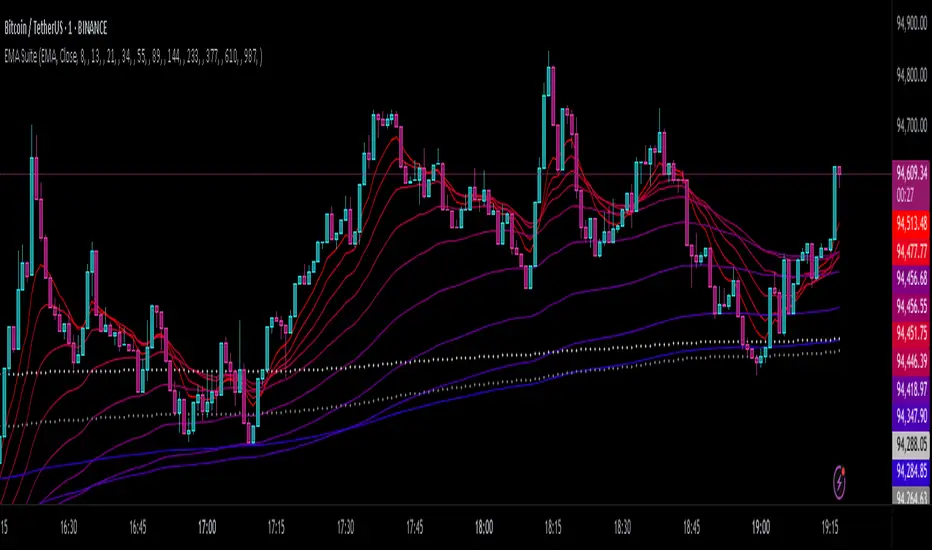
LinReg Heikin Ashi CandlesLinear Regression Heikin Ashi Candles will dramatically change how the candlesticks on your chart will appear. This script creates Heikin Ashi candles from the existing candlesticks and then applies wickless Linear Regression candles as an overlay. The result is an ultra smoothed 'Renko-like' chart that remains time-based and responsive.
Key Features:
Heikin Ashi Base: Provides a smoother representation of price trends by filtering out noise.
Linear Regression Candles on Heikin Ashi: Plots Linear Regression lines as candles on the Heikin Ashi chart, potentially highlighting the immediate trend direction and momentum within the smoothed data. Wicks are intentionally removed for a clearer focus on the linear progression.
Tillson T3 Moving Averages: Includes fast and slow T3 Moving Averages with customizable length and alpha. These smoothed moving averages can help identify trend direction and potential crossover signals. Users can toggle their visibility.
Volatility Bands: Integrates Volatility Bands based on Average True Range (ATR) with customizable length, ATR type (RMA, SMA, EMA, WMA), and inner/outer multipliers. These bands help gauge price volatility and potential reversal zones. Users can toggle the visibility of the basis line.
Customizable Colors: Allows users to customize the colors of the Linear Regression Heikin Ashi bullish and bearish candles.
How to Use:
This is an overlay on your chart so you'll need to 'hide' the existing candlesticks on your chart.
This indicator can be used on any timeframe from seconds to days to quickly identify market trend, gauge volatility, and potentially find entry/exit points. Consider looking for confluence between the candle color/direction, T3 MA crossovers, and price interaction with the Volatility Bands.
Note: This indicator plots Linear Regression directly on Heikin Ashi candles, removing wicks for a focus on the linear trend within the smoothed data. Adjust the input parameters to suit your trading style and the specific market conditions.
HUGE CREDIT to ugurvu who originally created the Linear Regression Candles indicator that my indicator pulls code from.
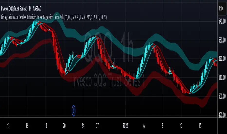
SuperTrend MTF Pro [Cometreon]The SuperTrend MTF Pro takes the classic SuperTrend to a whole new level of customization and accuracy. Unlike the standard version, this indicator allows you to select different moving averages, apply it to various chart types, and fine-tune every key parameter.
If you're looking for an advanced, non-repainting, and highly configurable SuperTrend, this is the right choice for you.
🔷 New Features and Improvements
🟩 Multi-MA SuperTrend
Now you can customize the SuperTrend calculation by choosing from 15 different moving averages:
SMA (Simple Moving Average)
EMA (Exponential Moving Average)
WMA (Weighted Moving Average)
RMA (Smoothed Moving Average)
HMA (Hull Moving Average)
JMA (Jurik Moving Average)
DEMA (Double Exponential Moving Average)
TEMA (Triple Exponential Moving Average)
LSMA (Least Squares Moving Average)
VWMA (Volume-Weighted Moving Average)
SMMA (Smoothed Moving Average)
KAMA (Kaufman’s Adaptive Moving Average)
ALMA (Arnaud Legoux Moving Average)
FRAMA (Fractal Adaptive Moving Average)
VIDYA (Variable Index Dynamic Average)
🟩 Multiple Chart Types
You're no longer limited to candlestick charts! Now you can use SuperTrend with different chart formats, including:
Heikin Ashi
Renko
Kagi
Line Break
Point & Figure
🟩 Customizable Timeframe
Now you can adjust the SuperTrend timeframe without repainting issues, avoiding signal distortions.
🔷 Technical Details and Customizable Inputs
SuperTrend offers multiple customization options to fit any trading strategy:
1️⃣ ATR Period – Defines the ATR length, affecting the indicator’s sensitivity.
2️⃣ Source – Selects the price value used for calculations (Close, HL2, Open, etc.).
3️⃣ ATR Mult – Multiplies the ATR to determine band distance. Higher values reduce false signals, lower values make it more reactive.
4️⃣ Change ATR Calculation Method – When enabled, uses the default ATR method; when disabled, allows selecting another Moving Average with "Use Different Type".
5️⃣ Source Break – Defines the price source for trend changes (Close for more stability, High/Low for more reactivity).
6️⃣ Use Different Type – Allows selecting an alternative Moving Average for ATR calculation if "Change ATR Calculation Method" is disabled.
7️⃣ SuperTrend Type – Advanced options for specific MAs (JMA, ALMA, FRAMA, VIDYA), with dedicated parameters like Phase, Sigma, and Offset for optimized responsiveness.
8️⃣ Ticker Settings – Customize parameters for special chart types such as Renko, Heikin Ashi, Kagi, Line Break, and Point & Figure, adjusting reversal, number of lines, and ATR length.
9️⃣ Timeframe – Enables using SuperTrend on a higher timeframe.
🔟 Wait for Timeframe Closes -
✅ Enabled – Prevents multiple signals, useful for precise alerts.
❌ Disabled – Displays SuperTrend smoothly without interruptions.
🔷 How to Use SuperTrend MTF Pro
🔍 Identifying Trends
SuperTrend follows the ongoing trend and provides clear visual signals:
When the price is above the line, the trend is bullish.
When the price is below the line, the trend is bearish.
📈 Interpreting Signals
Line color and position change → Possible trend reversal
Bounce off the line → Potential trend continuation
Strong breakout of the line → Possible reversal
🛠 Integration with Other Tools
RSI or MACD to filter false signals
Moving Averages to confirm trend direction
Support and Resistance to improve entry points
☄️ If you find this indicator useful, leave a Boost to support its development!
Every feedback helps to continuously improve the tool, offering an even more effective trading experience. Share your thoughts in the comments! 🚀🔥
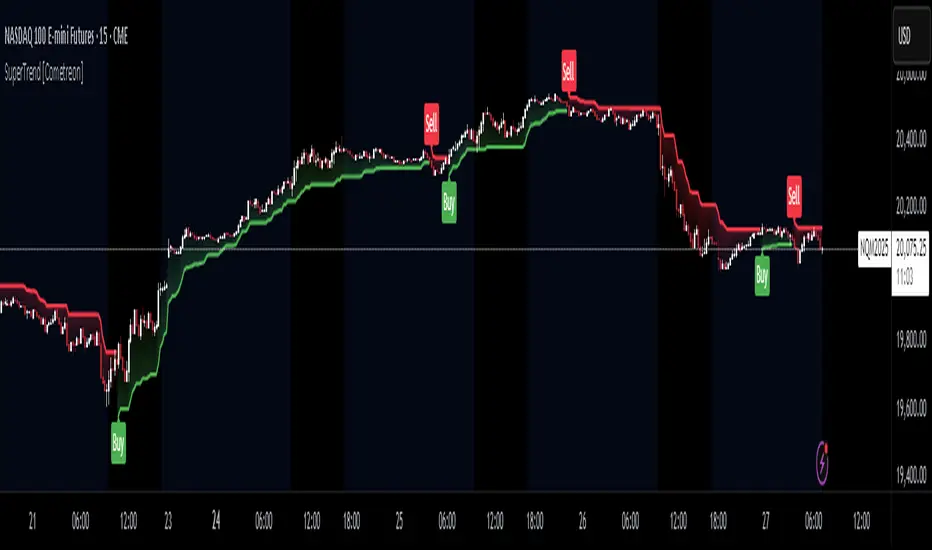
ST -Dashboard Volume MTF , [Sese04]User Guide: ST - Dashboard Volume MTF
Introduction
This script displays a multi-timeframe (MTF) volume dashboard, tracking buy and sell volumes and the moving averages of volume. It is designed for traders using ICT (Inner Circle Trader) and SMC (Smart Money Concepts) to quickly visualize market dynamics across multiple timeframes.
Settings and Features
📌 User Inputs
Customizable settings allow traders to adjust the dashboard display and volume moving averages.
Volume Display per Timeframe
show_vol_1m: Show volume for 1-minute chart.
show_vol_5m: Show volume for 5-minute chart.
show_vol_15m: Show volume for 15-minute chart.
show_vol_1h: Show volume for 1-hour chart.
show_vol_4h: Show volume for 4-hour chart.
show_vol_1d: Show volume for 1-day chart.
Volume Moving Average Settings
ma_length_short: Length of the short-term moving average (default 5 periods).
ma_length_long: Length of the long-term moving average (default 14 periods).
Dashboard Customization
dashboard_position: Dashboard position (Bottom Right, Bottom Left, Top Right, Top Left).
text_color: Text color for the dashboard.
text_size: Text size (small, normal, large).
How the Script Works
🔹 1. Calculating Buy and Sell Volume
The calculate_buy_sell function separates buy and sell volume based on the candle's open and close price:
If the closing price is higher than the opening price → Buy volume 📈.
If the closing price is lower or equal to the opening price → Sell volume 📉.
🔹 2. Retrieving Volume Data Across Multiple Timeframes
The function get_volumes collects buy and sell volume data for different timeframes using request.security().
The available timeframes are: 1m, 5m, 15m, 1h, 4h, and 1d.
🔹 3. Calculating Volume Moving Averages
The script uses ta.sma() to compute moving averages for volume trends:
ma_vol_short: Short-term moving average (e.g., 5 periods).
ma_vol_long: Long-term moving average (e.g., 14 periods).
🔹 4. Creating and Displaying the Dashboard
A table (table.new()) is generated at the last bar (barstate.islast) to display the volume data:
A title “📊 Volume Dashboard (Buy vs Sell)” in purple.
Column headers:
TIMEFRAME (e.g., 1M, 5M, 15M, 1H, 4H, 1D).
BUY VOLUME (dark blue).
SELL VOLUME (dark red).
Buy and Sell Volume values are displayed in their respective cells for easy reading.
How to Use This Script on TradingView?
Adding the Script
Open TradingView.
Go to Pine Editor and paste the script.
Click "Add to Chart".
Configuring the Settings
Open the indicator settings.
Enable/disable the desired timeframes.
Adjust the moving average lengths if necessary.
Interpreting the Data
Increasing buy volume across timeframes may indicate bullish momentum.
Rising sell volume suggests a bearish reversal.
Crossovers of volume moving averages can help detect market shifts.
Conclusion
This script is a powerful tool for analyzing volume dynamics across multiple timeframes. It provides a quick overview of the balance between buyers and sellers, essential for ICT scalping and liquidity-based trading.
🚀 Pro Tip: Combine this dashboard with other SMC indicators (engulfing candles, pivot points) to refine your trading decisions.

Relative Performance SuiteOverview
The Relative Performance Suite (RPS) is a versatile and comprehensive indicator designed to evaluate an asset's performance relative to a benchmark. By offering multiple methods to measure performance, including Relative Performance, Alpha, and Price Ratio, this tool helps traders and investors assess asset strength, resilience, and overall behavior in different market conditions.
Key Features:
✅ Multiple Performance Measures:
Choose from various relative performance calculations, including:
Relative Performance:
Measures how much an asset has outperformed or underperformed its benchmark over a given period.
Relative Performance (Proportional):
A proportional version of relative performance,
factoring in scaling effects.
Relative Performance (MA Based):
Uses moving averages to smooth performance fluctuations.
Alpha:
A measure of an asset’s performance relative to what would be expected based on its beta and the benchmark’s return. It represents the excess return above the risk-free rate after adjusting for market risk.
Price Ratio:
Compares asset prices directly to determine relative value over time.
✅ Customizable Moving Averages:
Apply different moving average types (SMA, EMA, SMMA, WMA, VWMA) to smooth price inputs and refine calculations.
✅ Beta Calculation:
Includes a Beta measure used in Alpha calculation, which users can toggle the visibility of helping users understand an asset's sensitivity to market movements.
✅ Risk-Free Rate Adjustment:
Incorporate risk-free rates (e.g., US Treasury yields, Fed Funds Rate) for a more accurate calculation of Alpha.
✅ Logarithmic Returns Option:
Users can switch between standard returns and log returns for more refined performance analysis.
✅ Dynamic Color Coding:
Identify outperformance or underperformance with intuitive color coding.
Option to color bars based on relative strength, making chart analysis easier.
✅ Customizable Tables for Data Display:
Overview table summarizing key metrics.
Explanation table offering insights into how values are derived.
How to Use:
Select a Benchmark: Choose a comparison symbol (e.g., TOTAL or SPX ).
Pick a Performance Metric: Use different modes to analyze relative performance.
Customize Calculation Methods: Adjust moving averages, timeframes, and log returns based on preference.
Interpret the Colors & Tables: Utilize the dynamic coloring and tables to quickly assess market conditions.
Ideal For:
Traders looking to compare individual asset performance against an index or benchmark.
Investors analyzing Alpha & Beta to understand risk-adjusted returns.
Market analysts who want a visually intuitive and data-rich performance tracking tool.
This indicator provides a powerful and flexible way to track relative asset strength, helping users make more informed trading decisions.

EMA/SMA Ribbon Pro (AUTO HTF + Labels)This indicator is a multi-timeframe (MTF) moving average ribbon that dynamically adjusts to the next highest timeframe. It provides a visual representation of market trends by stacking multiple EMAs and SMAs with customizable color fills and labels.
Features
✅ Multi-Timeframe (MTF) Support: Automatically detects the next highest time frame or allows for manual selection
✅ Customizable Moving Averages: Supports EMA and SMA with different lengths for flexible configuration
✅ Ribbon Visualization: Smooth color transitions between different moving averages for better trend identification
✅ Crossover Labels: Detects bullish and bearish EMA/SMA crossovers and marks them on the chart
✅ Price Labels & Timeframe Display: Displays moving average values to the right of the price axis with customizable label padding and colors
How It Works
Select the HTF mode: Manual or automatic
Choose EMA/SMA lengths to create different ribbons
Enable/disable price labels for each moving average
Customize colors and transparency for ribbons and labels
Crossover labels appear when faster moving averages cross slower ones and vice versa
Use Cases
📌 Trend Identification: Identify bullish and bearish trends using multiple EMAs and SMAs
📌 Support & Resistance Zones: MAs can act as dynamic support and resistance levels
📌 Reversal & Confirmation Signals: Watch for MTF crossovers to confirm trend changes
Customization
🔹 Standard EMA Lengths: 6, 8, 13, 21, 34, 48, 100, 200, 300, 400
🔹 SMA Lengths: 48, 100, 200
🔹 Color Adjustments: Set custom colors for bullish/bearish ribbons
🔹 Crossovers: Enable/disable custom crossover pairs (e.g., 100/200 EMA, 200 EMA/SMA).
This indicator is perfect for traders who rely on multi-timeframe confluence while seeking to enhance their market analysis and decision-making process.
As always, by combining EMA/SMA Ribbon with other tools, traders ensure that they are not relying on a single indicator. This layered approach can reduce the likelihood of false signals and improve overall trading accuracy.
As always, be sure to use any indicator with price action and volume indicators for better trade confirmation!

Moving Average Crossover StrategyCertainly! Below is an example of a professional trading strategy implemented in Pine Script for TradingView. This strategy is a simple moving average crossover strategy, which is a common approach used by many traders. It uses two moving averages (a short-term and a long-term) to generate buy and sell signals.
Input Parameters:
shortLength: The length of the short-term moving average.
longLength: The length of the long-term moving average.
Moving Averages:
shortMA: The short-term simple moving average (SMA).
longMA: The long-term simple moving average (SMA).
Conditions:
longCondition: A buy signal is generated when the short-term MA crosses above the long-term MA.
shortCondition: A sell signal is generated when the short-term MA crosses below the long-term MA.
Trade Execution:
The strategy enters a long position when the longCondition is met.
The strategy enters a short position when the shortCondition is met.
Plotting:
The moving averages are plotted on the chart.
Buy and sell signals are plotted as labels on the chart.
How to Use:
Copy the script into TradingView's Pine Script editor.
Adjust the shortLength and longLength parameters to fit your trading style.
Add the script to your chart and apply it to your desired timeframe.
Backtest the strategy to see how it performs on historical data.
This is a basic example, and professional traders often enhance such strategies with additional filters, risk management rules, and other indicators to improve performance.

Johnny's Machine Learning Moving Average (MLMA) w/ Trend Alerts📖 Overview
Johnny's Machine Learning Moving Average (MLMA) w/ Trend Alerts is a powerful adaptive moving average indicator designed to capture market trends dynamically. Unlike traditional moving averages (e.g., SMA, EMA, WMA), this indicator incorporates volatility-based trend detection, Bollinger Bands, ADX, and RSI, offering a comprehensive view of market conditions.
The MLMA is "machine learning-inspired" because it adapts dynamically to market conditions using ATR-based windowing and integrates multiple trend strength indicators (ADX, RSI, and volatility bands) to provide an intelligent moving average calculation that learns from recent price action rather than being static.
🛠 How It Works
1️⃣ Adaptive Moving Average Selection
The MLMA automatically selects one of four different moving averages:
📊 EMA (Exponential Moving Average) – Reacts quickly to price changes.
🔵 HMA (Hull Moving Average) – Smooth and fast, reducing lag.
🟡 WMA (Weighted Moving Average) – Gives recent prices more importance.
🔴 VWAP (Volume Weighted Average Price) – Accounts for volume impact.
The user can select which moving average type to use, making the indicator customizable based on their strategy.
2️⃣ Dynamic Trend Detection
ATR-Based Adaptive Window 📏
The Average True Range (ATR) determines the window size dynamically.
When volatility is high, the moving average window expands, making the MLMA more stable.
When volatility is low, the window shrinks, making the MLMA more responsive.
Trend Strength Filters 📊
ADX (Average Directional Index) > 25 → Indicates a strong trend.
RSI (Relative Strength Index) > 70 or < 30 → Identifies overbought/oversold conditions.
Price Position Relative to Upper/Lower Bands → Determines bullish vs. bearish momentum.
3️⃣ Volatility Bands & Dynamic Support/Resistance
Bollinger Bands (BB) 📉
Uses standard deviation-based bands around the MLMA to detect overbought and oversold zones.
Upper Band = Resistance, Lower Band = Support.
Helps traders identify breakout potential.
Adaptive Trend Bands 🔵🔴
The MLMA has built-in trend envelopes.
When price breaks the upper band, bullish momentum is confirmed.
When price breaks the lower band, bearish momentum is confirmed.
4️⃣ Visual Enhancements
Dynamic Gradient Fills 🌈
The trend strength (ADX-based) determines the gradient intensity.
Stronger trends = More vivid colors.
Weaker trends = Lighter colors.
Trend Reversal Arrows 🔄
🔼 Green Up Arrow: Bullish reversal signal.
🔽 Red Down Arrow: Bearish reversal signal.
Trend Table Overlay 🖥
Displays ADX, RSI, and Trend State dynamically on the chart.
📢 Trading Signals & How to Use It
1️⃣ Bullish Signals 📈
✅ Conditions for a Long (Buy) Trade:
The MLMA crosses above the lower band.
The ADX is above 25 (confirming trend strength).
RSI is above 55, indicating positive momentum.
Green trend reversal arrow appears (confirmation of a bullish reversal).
🔹 How to Trade It:
Enter a long trade when the MLMA turns bullish.
Set stop-loss below the lower Bollinger Band.
Target previous resistance levels or use the upper band as take-profit.
2️⃣ Bearish Signals 📉
✅ Conditions for a Short (Sell) Trade:
The MLMA crosses below the upper band.
The ADX is above 25 (confirming trend strength).
RSI is below 45, indicating bearish pressure.
Red trend reversal arrow appears (confirmation of a bearish reversal).
🔹 How to Trade It:
Enter a short trade when the MLMA turns bearish.
Set stop-loss above the upper Bollinger Band.
Target the lower band as take-profit.
💡 What Makes This a Machine Learning Moving Average?
📍 1️⃣ Adaptive & Self-Tuning
Unlike static moving averages that rely on fixed parameters, this MLMA automatically adjusts its sensitivity to market conditions using:
ATR-based dynamic windowing 📏 (Expands/contracts based on volatility).
Adaptive smoothing using EMA, HMA, WMA, or VWAP 📊.
Multi-indicator confirmation (ADX, RSI, Volatility Bands) 🏆.
📍 2️⃣ Intelligent Trend Confirmation
The MLMA "learns" from recent price movements instead of blindly following a fixed-length average.
It incorporates ADX & RSI trend filtering to reduce noise & false signals.
📍 3️⃣ Dynamic Color-Coding for Trend Strength
Strong trends trigger more vivid colors, mimicking confidence levels in machine learning models.
Weaker trends appear faded, suggesting uncertainty.
🎯 Why Use the MLMA?
✅ Pros
✔ Combines multiple trend indicators (MA, ADX, RSI, BB).
✔ Automatically adjusts to market conditions.
✔ Filters out weak trends, making it more reliable.
✔ Visually intuitive (gradient colors & reversal arrows).
✔ Works across all timeframes and assets.
⚠️ Cons
❌ Not a standalone strategy → Best used with volume confirmation or candlestick analysis.
❌ Can lag slightly in fast-moving markets (due to smoothing).
