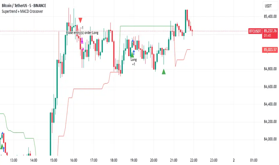
Supertrend + MACD CrossoverKey Elements of the Template:
Supertrend Settings:
supertrendFactor: Adjustable to control the sensitivity of the Supertrend.
supertrendATRLength: ATR length used for Supertrend calculation.
MACD Settings:
macdFastLength, macdSlowLength, macdSignalSmoothing: These settings allow you to fine-tune the MACD for better results.
Risk Management:
Stop-Loss: The stop-loss is based on the ATR (Average True Range), a volatility-based indicator.
Take-Profit: The take-profit is based on the risk-reward ratio (set to 3x by default).
Both stop-loss and take-profit are dynamic, based on ATR, which adjusts according to market volatility.
Buy and Sell Signals:
Buy Signal: Supertrend is bullish, and MACD line crosses above the Signal line.
Sell Signal: Supertrend is bearish, and MACD line crosses below the Signal line.
Visual Elements:
The Supertrend line is plotted in green (bullish) and red (bearish).
Buy and Sell signals are shown with green and red triangles on the chart.
Next Steps for Optimization:
Backtesting:
Run backtests on BTC in the 5-minute timeframe and adjust parameters (Supertrend factor, MACD settings, risk-reward ratio) to find the optimal configuration for the 60% win ratio.
Fine-Tuning Parameters:
Adjust supertrendFactor and macdFastLength to find more optimal values based on BTC's market behavior.
Tweak the risk-reward ratio to maximize profitability while maintaining a good win ratio.
Evaluate Market Conditions:
The performance of the strategy can vary based on market volatility. It may be helpful to evaluate performance in different market conditions or pair it with a filter like RSI or volume.
Let me know if you'd like further tweaks or explanations!
Cerca negli script per "backtest"
[TehThomas] - Displacement CandlesOverview:
This PineScript is designed to detect and visualize significant price movements, called displacements, on a trading chart. It's particularly useful for traders who want to identify potential trend changes or strong market sentiment quickly.
How the Script Works
User Input:
The script allows users to set a custom threshold for displacement detection and choose colors for bullish and bearish movements.
Displacement Detection Function:
isDisplacement(series, threshold) =>
percentage_change = math.abs(series - series ) / series * 100
percentage_change > threshold
This function calculates the percentage change between the current and previous price.
If the change exceeds the set threshold, it's considered a displacement.
Bullish and Bearish Detection:
bullish_displacement = isDisplacement(close, threshold) and close > close
bearish_displacement = isDisplacement(close, threshold) and close < close
Identifies whether the displacement is bullish (price increase) or bearish (price decrease).
Candle Coloring:
barcolor(bullish_displacement ? bullish_color : bearish_displacement ? bearish_color : na)
Changes the color of candles based on the detected displacement type.
Usefulness and Applications:
Trend Identification: Helps in quickly spotting potential trend changes or continuations.
Volatility Analysis: Provides a visual representation of market volatility.
Entry and Exit Signals: Can be used to identify potential entry or exit points for trades.
Market Sentiment: Offers insights into the strength of bullish or bearish sentiment.
Customizable Sensitivity: The adjustable threshold allows traders to fine-tune the indicator based on the asset's typical volatility.
Visual Clarity: By changing candle colors, it provides a clear, at-a-glance view of significant price movements.
Complementary Tool: Can be used alongside other technical indicators for confirmation of signals.
Multiple Timeframe Analysis: Applicable across different timeframes to suit various trading styles (day trading, swing trading, etc.).
Educational Purpose: Helps new traders understand and visualize significant price movements in the market.
Backtesting: Can be incorporated into strategy backtests to assess its effectiveness in different market conditions.
This script is particularly handy for traders who want to cut through market noise and focus on significant price movements. It's versatile enough to be used across different trading strategies and can be a valuable addition to a trader's technical analysis toolkit.
It's a very easy script and not alot to mention. If you see any improvements please let me know.

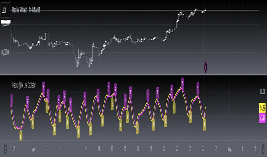
[blackcat] L1 Main life line oscillator█ OVERVIEW
The Pine Script provided is an indicator named " L1 Main life line oscillator." Its primary function is to calculate and plot two oscillators: the Main Force and the Life Line. These oscillators are derived from smoothed price data, and the script also detects and labels crossovers and crossunders between the two lines, which can be used to generate buy and sell signals.
█ FEATURES
Key Features:
• Input Parameters: Users can define the period (n) and the weight for the oscillators.
• Custom Function: A function calculate_life_line_oscillator is defined to compute the Main Force and Life Line oscillators.
• Advanced Calculations: The script uses an adaptive moving average (ALMA) and exponential moving average (EMA) to smooth the price data and calculate the oscillators.
• Crossover and Crossunder Detection: Built-in functions ta.crossover and ta.crossunder are used to identify signal points.
• Label Drawing: Custom labels are drawn on the chart to indicate buy ("B") and sell ("S") signals.
█ HOW TO USE
1 — Configure Input Parameters: Adjust the period (n) and weight to suit your trading strategy.
2 — Interpret the Oscillators: Observe the Main Force and Life Line on the chart.
3 — Act on Signals: Look for crossovers and crossunders to generate buy and sell signals. Buy signals are indicated by the label "B" and sell signals by "S".
█ LIMITATIONS
• Lag in Signals: While the use of ALMA and EMA reduces lag, some delay may still occur, especially in volatile markets.
• False Signals: Crossovers and crossunders can sometimes produce false signals, so it is advisable to use this indicator in conjunction with other tools for confirmation.
█ NOTES
Advanced Pine Script Features:
• Adaptive Moving Average (ALMA): Provides a more responsive and adaptive oscillator.
• Exponential Moving Average (EMA): Smooths the price range and Main Force values.
• Crossover and Crossunder Detection: Utilizes built-in functions for signal identification.
• Label Drawing: Enhances visual signaling with custom labels.
Optimization Techniques:
• The use of ALMA and EMA helps in reducing lag and improving the responsiveness of the oscillators.
• The custom function encapsulates complex calculations, making the main script cleaner and more maintainable.
Unique Approaches:
• The combination of ALMA and EMA to create the Main Force oscillator provides a unique smoothing method.
• The Life Line is calculated using a weighted average of the previous and current Main Force values, adding an additional layer of smoothing and responsiveness.
█ THANKS
Thank you for using the " L1 Main life line oscillator." If you have any questions or suggestions, please feel free to reach out in the comments or on the TradingView or my Discord channel.
█ EXTENDED KNOWLEDGE AND APPLICATIONS
Potential Modifications:
• Additional Indicators: Extend the script to include other technical indicators (e.g., RSI, MACD) for a more comprehensive trading signal system.
• Customizable Colors and Styles: Allow users to customize the colors and styles of the plotted lines and labels.
• Alerts: Implement alerts for crossovers and crossunders to notify users in real-time.
Application Scenarios:
• Intraday Trading: The responsiveness of the oscillators makes this script suitable for intraday trading, where quick buy and sell signals are crucial.
• Long-Term Analysis: By adjusting the period n, the script can be used for long-term trend analysis and strategic trades.
• Backtesting: The script can be modified into a strategy to backtest the performance of the oscillator-based signals against historical data.
Related Pine Script Concepts:
• Strategy Development: Understanding how to convert indicators into strategies for backtesting and live trading.
• Advanced Plotting: Exploring more advanced plotting techniques, such as using different styles and customizing plot appearances.
• Signal Validation: Techniques for validating and filtering signals to reduce false positives and improve trade accuracy.
Equilibrium Candles + Pattern [Honestcowboy]The Equilibrium Candles is a very simple trend continuation or reversal strategy depending on your settings.
How an Equilibrium Candle is created:
We calculate the equilibrium by measuring the mid point between highest and lowest point over X amount of bars back.
This now is the opening price for each bar and will be considered a green bar if price closes above equilibrium.
Bars get shaded by checking if regular candle close is higher than open etc. So you still see what the normal candles are doing.
Why are they useful?
The equilibrium is calculated the same as Baseline in Ichimoku Cloud. Which provides a point where price is very likely to retrace to. This script visualises the distance between close and equilibrium using candles. To provide a clear visual of how price relates to this equilibrium point.
This also makes it more straightforward to develop strategies based on this simple concept and makes the trader purely focus on this relationship and not think of any Ichimoku Cloud theories.
Script uses a very simple pattern to enter trades:
It will count how many candles have been one directional (above or below equilibrium)
Based on user input after X candles (7 by default) script shows we are in a trend (bg colors)
On the first pullback (candle closes on other side of equilibrium) it will look to enter a trade.
Places a stop order at the high of the candle if bullish trend or reverse if bearish trend.
If based on user input after X opposite candles (2 by default) order is not filled will cancel it and look for a new trend.
Use Reverse Logic:
There is a use reverse logic in the settings which on default is turned on. It will turn long orders into short orders making the stop orders become limit orders. It will use the normal long SL as target for the short. And TP as stop for the short. This to provide a means to reverse equity curve in case your pair is mean reverting by nature instead of trending.
ATR Calculation:
Averaged ATR, which is using ta.percentile_nearest_rank of 60% of a normal ATR (14 period) over the last 200 bars. This in simple words finds a value slightly above the mean ATR value over that period.
Big Candle Exit Logic:
Using Averaged ATR the script will check if a candle closes X times that ATR from the equilibrium point. This is then considered an overextension and all trades are closed.
This is also based on user input.
Simple trade management logic:
Checks if the user has selected to use TP and SL, or/and big candle exit.
Places a TP and SL based on averaged ATR at a multiplier based on user Input.
Closes trade if there is a Big Candle Exit or an opposite direction signal from indicator.
Script can be fully automated to MT5
There are risk settings in % and symbol settings provided at the bottom of the indicator. The script will send alert to MT5 broker trying to mimic the execution that happens on tradingview. There are always delays when using a bridge to MT5 broker and there could be errors so be mindful of that. This script sends alerts in format so they can be read by tradingview.to which is a bridge between the platforms.
Use the all alert function calls feature when setting up alerts and make sure you provide the right webhook if you want to use this approach.
There is also a simple buy and sell alert feature if you don't want to fully automate but still get alerts. These are available in the dropdown when creating an alert.
Almost every setting in this indicator has a tooltip added to it. So if any setting is not clear hover over the (?) icon on the right of the setting.
The backtest uses a 4% exposure per trade and a 10 point slippage. I did not include a commission cause I'm not personaly aware what the commissions are on most forex brokers. I'm only aware of minimal slippage to use in a backtest. Trading conditions vary per broker you use so always pay close attention to trading costs on your own broker. Use a full automation at your own risk and discretion and do proper backtesting.

TradingView.To Strategy Template (with Dyanmic Alerts)Hello traders,
If you're tired of manual trading and looking for a solid strategy template to pair with your indicators, look no further.
This Pine Script v5 strategy template is engineered for maximum customization and risk management.
Best part?
This Pine Script v5 template facilitates the dynamic construction of TradingView.TO alerts, sparing users the time and effort of mastering the TradingView.TO syntax and manually create alert commands.
This powerful tool gives much power to those who don't know how to code in Pinescript and want to automate their indicators' signals via TradingView.TO bot.
IMPORTANT NOTES
TradingView.TO is a trading bot software that forwards TradingView alerts to your brokers (examples: Binance, Oanda, Coinbase, Bybit, Metatrader 4/5, ...) for automating trading.
Many traders don't know how to create TradingView.TO dynamically-compatible alerts using the data from their TradingView scripts.
Traders using trading bots want their alerts to reflect the stop-loss/take-profit/trailing-stop/stop-loss to break options from your script and then create the orders accordingly.
This script showcases how to create TradingView.TO alerts dynamically.
TRADINGVIEW ALERTS
1) You'll have to create one alert per asset X timeframe = 1 chart.
Example: 1 alert for BTC/USDT on the 5 minutes chart, 1 alert for BTC/USDT on the 15-minute chart (assuming you want your bot to trade the BTC/USDT on the 5 and 15-minute timeframes)
2) Select the Order fills and alert() function calls condition
3) For each alert, the alert message is pre-configured with the text below
{{strategy.order.alert_message}}
Please leave it as it is.
It's a TradingView native variable that will fetch the alert text messages built by the script.
4) TradingView.TO uses webhook technology - setting a webhook URL from the alerts notifications tab is required.
KEY FEATURES
I) Modular Indicator Connection
* plug your existing indicator into the template.
* Only two lines of code are needed for full compatibility.
Step 1: Create your connector
Adapt your indicator with only 2 lines of code and then connect it to this strategy template.
To do so:
1) Find in your indicator where the conditions print the long/buy and short/sell signals.
2) Create an additional plot as below
I'm giving an example with a Two moving averages cross.
Please replicate the same methodology for your indicator, whether a MACD , ZigZag, Pivots , higher-highs, lower-lows or whatever indicator with clear buy and sell conditions.
//@version=5
indicator("Supertrend", overlay = true, timeframe = "", timeframe_gaps = true)
atrPeriod = input.int(10, "ATR Length", minval = 1)
factor = input.float(3.0, "Factor", minval = 0.01, step = 0.01)
= ta.supertrend(factor, atrPeriod)
supertrend := barstate.isfirst ? na : supertrend
bodyMiddle = plot(barstate.isfirst ? na : (open + close) / 2, display = display.none)
upTrend = plot(direction < 0 ? supertrend : na, "Up Trend", color = color.green, style = plot.style_linebr)
downTrend = plot(direction < 0 ? na : supertrend, "Down Trend", color = color.red, style = plot.style_linebr)
fill(bodyMiddle, upTrend, color.new(color.green, 90), fillgaps = false)
fill(bodyMiddle, downTrend, color.new(color.red, 90), fillgaps = false)
buy = ta.crossunder(direction, 0)
sell = ta.crossunder(direction, 0)
//////// CONNECTOR SECTION ////////
Signal = buy ? 1 : sell ? -1 : 0
plot(Signal, title = "Signal", display = display.data_window)
//////// CONNECTOR SECTION ////////
Important Notes
🔥 The Strategy Template expects the value to be exactly 1 for the bullish signal and -1 for the bearish signal
Now, you can connect your indicator to the Strategy Template using the method below or that one.
Step 2: Connect the connector
1) Add your updated indicator to a TradingView chart
2) Add the Strategy Template as well to the SAME chart
3) Open the Strategy Template settings, and in the Data Source field, select your 🔌Connector🔌 (which comes from your indicator)
Note it doesn’t have to be named 🔌Connector🔌 - you can name it as you want - however, I recommend an explicit name you can easily remember.
From then, you should start seeing the signals and plenty of other stuff on your chart.
🔥 Note that whenever you update your indicator values, the strategy statistics and visuals on your chart will update in real-time
II) BOT Risk Management:
- Max Drawdown:
Mode: Select whether the max drawdown is calculated in percentage (%) or USD.
Value: If the max drawdown reaches this specified value, set a value to halt the bot.
- Max Consecutive Days:
Use Max Consecutive Days BOT Halt: Enable/Disable halting the bot if the max consecutive losing days value is reached.
- Max Consecutive Days: Set the maximum number of consecutive losing days allowed before halting the bot.
- Max Losing Streak:
Use Max Losing Streak: Enable/Disable a feature to prevent the bot from taking too many losses in a row.
- Max Losing Streak Length: Set the maximum length of a losing streak allowed.
Margin Call:
- Use Margin Call: Enable/Disable a feature to exit when a specified percentage away from a margin call to prevent it.
Margin Call (%): Set the percentage value to trigger this feature.
- Close BOT Total Loss:
Use Close BOT Total Loss: Enable/Disable a feature to close all trades and halt the bot if the total loss is reached.
- Total Loss ($): Set the total loss value in USD to trigger this feature.
Intraday BOT Risk Management:
- Intraday Losses:
Use Intraday Losses BOT Halt: Enable/Disable halting the bot on reaching specified intraday losses.
Mode: Select whether the intraday loss is calculated in percentage (%) or USD.
- Max Intraday Losses (%): Set the value for maximum intraday losses.
Limit Intraday Trades:
- Use Limit Intraday Trades: Enable/Disable a feature to limit the number of intraday trades.
- Max Intraday Trades: Set the maximum number of intraday trades allowed.
Restart Intraday EA:
III) Order Types and Position Sizing
- Choose between market or limit orders.
- Set your position size directly in the template.
Please use the position size from the “Inputs” and not the “Properties” tab.
I know it's redundant. - the template needs this value from the "Inputs" tab to build the alerts, and the Backtester needs it from the "Properties" tab.
IV) Advanced Take-Profit and Stop-Loss Options
- Choose to set your SL/TP in either USD or percentages.
- Option for multiple take-profit levels and trailing stop losses.
- Move your stop loss to break even +/- offset in USD for “risk-free” trades.
V) Miscellaneous:
Retry order openings if they fail.
Order Types:
Select and specify order type and price settings.
Position Size:
Define the type and size of positions.
Leverage:
Leverage settings, including margin type and hedge mode.
Session:
Limit trades to specific sessions.
Dates:
Limit trades to a specific date range.
Trades Direction:
Direction: Specify the market direction for opening positions.
VI) Logger
The TradingView.TO commands are logged in the TradingView logger.
You'll find more information about it in this TradingView blog post .
WHY YOU MIGHT NEED THIS TEMPLATE
1) Transform your indicator into a TradingView.TO trading bot more easily than before
Connect your indicator to the template
Create your alerts
Set your EA settings
2) Save Time
Auto-generated alert messages for TradingView.TO.
I tested them all and checked with the support team what could/couldn’t be done.
3) Be in Control
Manage your trading risks with advanced features.
4) Customizable
Fits various trading styles and asset classes.
REQUIREMENTS
* Make sure you have your TradingView.TO account
* If there is any issue with the template, ask me in the comments section - I’ll answer quickly.
BACKTEST RESULTS FROM THIS POST
1) I connected this strategy template to a dummy Supertrend script.
I could have selected any other indicator or concept for this script post.
I wanted to share an example of how you can quickly upgrade your strategy, making it compatible with TradingView.TO.
2) The backtest results aren't relevant for this educational script publication.
I used realistic backtesting data but didn't look too much into optimizing the results, as this isn't the point of why I'm publishing this script.
This strategy is a template to be connected to any indicator - the sky is the limit. :)
3) This template is made to take 1 trade per direction at any given time.
Pyramiding is set to 1 on TradingView.
The strategy default settings are:
* Initial Capital: 100000 USD
* Position Size: 1%
* Commission Percent: 0.075%
* Slippage: 1 tick
* No margin/leverage used

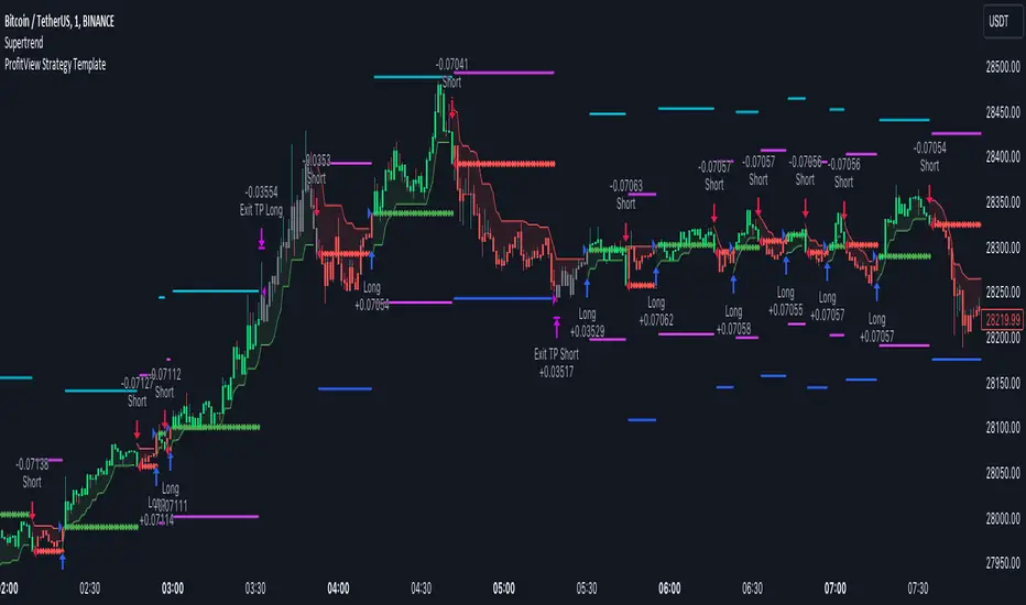
ProfitView Strategy TemplateHello traders,
This script took me a full week of coding/testing, sweat, and tears - and I’m too nice as I’m giving it for free to the community.
If you're tired of manual trading and looking for a solid strategy template to pair with your indicators, look no further.
This Pine Script v5 strategy template is engineered for maximum customization and risk management.
Best part?
This Pine Script v5 template facilitates the dynamic construction of ProfitView alerts, sparing users the time and effort of mastering the ProfitView syntax and manually creating alert commands.
This powerful tool gives much power to those who don't know how to code in Pinescript and want to automate their indicators' signals via the ProfitView Chrome extension.
IMPORTANT NOTES
ProfitView is a trading bot software that forwards TradingView alerts to your brokers (examples: Binance, Oanda, Coinbase, Bybit, etc.) for automating trading.
Many traders don't know how to dynamically create ProfitView-compatible alerts using the data from their TradingView scripts.
Traders using trading bots want their alerts to reflect the stop-loss/take-profit/trailing-stop/stop-loss to break options from your script and then create the orders accordingly.
This script showcases how to create ProfitView alerts dynamically.
TRADINGVIEW ALERTS
1) You'll have to create one alert per asset X timeframe = 1 chart.
Example: 1 alert for EUR/USD on the 5 minutes chart, 1 alert for EUR/USD on the 15-minute chart (assuming you want your bot to trade the EUR/USD on the 5 and 15-minute timeframes)
2) Select the Order fills and alert() function calls condition
3) For each alert, the alert message is pre-configured with the text below
{{strategy.order.alert_message}}
Please leave it as it is.
It's a TradingView native variable that will fetch the alert text messages built by the script.
4) ProfitView doesn't use webhook technology, so setting a webhook URL from the alerts notifications tab is unnecessary.
KEY FEATURES
I) Modular Indicator Connection
* plug your existing indicator into the template.
* Only two lines of code are needed for full compatibility.
Step 1: Create your connector
Adapt your indicator with only 2 lines of code and then connect it to this strategy template.
To do so:
1) Find in your indicator where the conditions print the long/buy and short/sell signals.
2) Create an additional plot as below
I'm giving an example with a Two moving averages cross.
Please replicate the same methodology for your indicator, whether a MACD , ZigZag, Pivots , higher-highs, lower-lows or whatever indicator with clear buy and sell conditions.
//@version=5
indicator("Supertrend", overlay = true, timeframe = "", timeframe_gaps = true)
atrPeriod = input.int(10, "ATR Length", minval = 1)
factor = input.float(3.0, "Factor", minval = 0.01, step = 0.01)
= ta.supertrend(factor, atrPeriod)
supertrend := barstate.isfirst ? na : supertrend
bodyMiddle = plot(barstate.isfirst ? na : (open + close) / 2, display = display.none)
upTrend = plot(direction < 0 ? supertrend : na, "Up Trend", color = color.green, style = plot.style_linebr)
downTrend = plot(direction < 0 ? na : supertrend, "Down Trend", color = color.red, style = plot.style_linebr)
fill(bodyMiddle, upTrend, color.new(color.green, 90), fillgaps = false)
fill(bodyMiddle, downTrend, color.new(color.red, 90), fillgaps = false)
buy = ta.crossunder(direction, 0)
sell = ta.crossunder(direction, 0)
//////// CONNECTOR SECTION ////////
Signal = buy ? 1 : sell ? -1 : 0
plot(Signal, title = "Signal", display = display.data_window)
//////// CONNECTOR SECTION ////////
Important Notes
🔥 The Strategy Template expects the value to be exactly 1 for the bullish signal and -1 for the bearish signal
Now, you can connect your indicator to the Strategy Template using the method below or that one.
Step 2: Connect the connector
1) Add your updated indicator to a TradingView chart
2) Add the Strategy Template as well to the SAME chart
3) Open the Strategy Template settings, and in the Data Source field, select your 🔌Connector🔌 (which comes from your indicator)
Note it doesn’t have to be named 🔌Connector🔌 - you can name it as you want - however, I recommend an explicit name you can easily remember.
From then, you should start seeing the signals and plenty of other stuff on your chart.
🔥 Note that whenever you update your indicator values, the strategy statistics and visuals on your chart will update in real-time
II) BOT Risk Management:
- Max Drawdown:
Mode: Select whether the max drawdown is calculated in percentage (%) or USD.
Value: If the max drawdown reaches this specified value, set a value to halt the bot.
- Max Consecutive Days:
Use Max Consecutive Days BOT Halt: Enable/Disable halting the bot if the max consecutive losing days value is reached.
- Max Consecutive Days: Set the maximum number of consecutive losing days allowed before halting the bot.
- Max Losing Streak:
Use Max Losing Streak: Enable/Disable a feature to prevent the bot from taking too many losses in a row.
- Max Losing Streak Length: Set the maximum length of a losing streak allowed.
Margin Call:
- Use Margin Call: Enable/Disable a feature to exit when a specified percentage away from a margin call to prevent it.
Margin Call (%): Set the percentage value to trigger this feature.
- Close BOT Total Loss:
Use Close BOT Total Loss: Enable/Disable a feature to close all trades and halt the bot if the total loss is reached.
- Total Loss ($): Set the total loss value in USD to trigger this feature.
Intraday BOT Risk Management:
- Intraday Losses:
Use Intraday Losses BOT Halt: Enable/Disable halting the bot on reaching specified intraday losses.
Mode: Select whether the intraday loss is calculated in percentage (%) or USD.
- Max Intraday Losses (%): Set the value for maximum intraday losses.
Limit Intraday Trades:
- Use Limit Intraday Trades: Enable/Disable a feature to limit the number of intraday trades.
- Max Intraday Trades: Set the maximum number of intraday trades allowed.
Restart Intraday EA:
- Use Restart Intraday EA: Enable/Disable a feature to restart the bot at the first bar of the next day if it has been stopped with an intraday risk management safeguard.
III) Order Types and Position Sizing
- Choose between market, limit, or stop orders.
- Set your position size directly in the template.
Please use the position size from the “Inputs” and not the “Properties” tab.
I know it's redundant. - the template needs this value from the "Inputs" tab to build the alerts, and the Backtester needs it from the "Properties" tab.
IV) Advanced Take-Profit and Stop-Loss Options
- Choose to set your SL/TP in either pips or percentages.
- Option for multiple take-profit levels and trailing stop losses.
- Move your stop loss to break even +/- offset in pips for “risk-free” trades.
V) Miscellaneous
Retry order openings if they fail.
Order Types:
Select and specify order type and price settings.
Position Size:
Define the type and size of positions.
Leverage:
Leverage settings, including margin type and hedge mode.
Session:
Limit trades to specific sessions.
Dates:
Limit trades to a specific date range.
Trades Direction:
Direction: Specify the market direction for opening positions.
VI) Notifications (Telegram/Discord/Email/IFTTT/Twilio/SMS)
Customize notifications sent to Telegram, Discord, Email, IFTTT, Twilio, and ProfitView Logger.
VII) Logger
The ProfitView commands are logged in the TradingView logger.
You'll find more information about it in this TradingView blog post .
WHY YOU MIGHT NEED THIS TEMPLATE
1) Transform your indicator into a ProfitView trading bot more easily than before
Connect your indicator to the template
Create your alerts
Set your EA settings
2) Save Time
Auto-generated alert messages for ProfitView.
I tested them all and checked with the support team what could/couldn’t be done.
3) Be in Control
Manage your trading risks with advanced features.
4) Customizable
Fits various trading styles and asset classes.
REQUIREMENTS
* Make sure you have your ProfitView account and do the settings correctly in your Chrome extension. If you don't know how to do it, read the documentation + ask for help in the ProfitView Discord support channel.
* If there is any issue with the template, ask me in the comments section - I’ll answer quickly.
BACKTEST RESULTS FROM THIS POST
1) I connected this strategy template to a dummy Supertrend script.
I could have selected any other indicator or concept for this script post.
I wanted to share an example of how you can quickly upgrade your strategy, making it compatible with ProfitView.
2) The backtest results aren't relevant for this educational script publication.
I used realistic backtesting data but didn't look too much into optimizing the results, as this isn't the point of why I'm publishing this script.
This strategy is a template to be connected to any indicator - the sky is the limit. :)
3) This template is made to take 1 trade per direction at any given time.
Pyramiding is set to 1 on TradingView.
The strategy default settings are:
* Initial Capital: 100000 USD
* Position Size: 1%
* Commission Percent: 0.075%
* Slippage: 1 tick
* No margin/leverage used
Best regards,
Dave
EMA bands + leledc + bollinger bands trend following strategy v2The basics:
In its simplest form, this strategy is a positional trend following strategy which enters long when price breaks out above "middle" EMA bands and closes or flips short when price breaks down below "middle" EMA bands. The top and bottom of the middle EMA bands are calculated from the EMA of candle highs and lows, respectively.
The idea is that entering trades on breakouts of the high EMAs and low EMAs rather than the typical EMA based on candle closes gives a bit more confirmation of trend strength and minimizes getting chopped up. To further reduce getting chopped up, the strategy defaults to close on crossing the opposite EMA band (ie. long on break above high EMA middle band and close below low EMA middle band).
This strategy works on all markets on all timeframes, but as a trend following strategy it works best on markets prone to trending such as crypto and tech stocks. On lower timeframes, longer EMAs tend to work best (I've found good results on EMA lengths even has high up to 1000), while 4H charts and above tend to work better with EMA lengths 21 and below.
As an added filter to confirm the trend, a second EMA can be used. Inputting a slower EMA filter can ensure trades are entered in accordance with longer term trends, inputting a faster EMA filter can act as confirmation of breakout strength.
Bar coloring can be enabled to quickly visually identify a trend's direction for confluence with other indicators or strategies.
The goods:
Waiting for the trend to flip before closing a trade (especially when a longer base EMA is used) often leaves money on the table. This script combines a number of ways to identify when a trend is exhausted for backtesting the best early exits.
"Delayed bars inside middle bands" - When a number of candle's in a row open and close between the middle EMA bands, it could be a sign the trend is weak, or that the breakout was not the start of a new trend. Selecting this will close out positions after a number of bars has passed
"Leledc bars" - Originally introduced by glaz, this is a price action indicator that highlights a candle after a number of bars in a row close the same direction and result in greatest high/low over a period. It often triggers when a strong trend has paused before further continuation, or it marks the end of a trend. To mitigate closing on false Leledc signals, this strategy has two options: 1. Introducing requirement for increased volume on the Leledc bars can help filter out Leledc signals that happen mid trend. 2. Closing after a number of Leledc bars appear after position opens. These two options work great in isolation but don't perform well together in my testing.
"Bollinger Bands exhaustion bars" - These bars are highlighted when price closes back inside the Bollinger Bands and RSI is within specified overbought/sold zones. The idea is that a trend is overextended when price trades beyond the Bollinger Bands. When price closes back inside the bands it's likely due for mean reversion back to the base EMA in which this strategy will ideally re-enter a position. Since the added RSI requirements often make this indicator too strict to trigger a large enough sample size to backtest, I've found it best to use "non-standard" settings for both the bands and the RSI as seen in the default settings.
"Buy/Sell zones" - Similar to the idea behind using Bollinger Bands exhaustion bars as a closing signal. Instead of calculating off of standard deviations, the Buy/Sell zones are calculated off multiples of the middle EMA bands. When trading beyond these zones and subsequently failing back inside, price may be due for mean reversion back to the base EMA. No RSI filter is used for Buy/Sell zones.
If any early close conditions are selected, it's often worth enabling trade re-entry on "middle EMA band bounce". Instead of waiting for a candle to close back inside the middle EMA bands, this feature will re-enter position on only a wick back into the middle bands as will sometimes happen when the trend is strong.
Any and all of the early close conditions can be combined. Experimenting with these, I've found can result in less net profit but higher win-rates and sharpe ratios as less time is spent in trades.
The deadly:
The trend is your friend. But wouldn't it be nice to catch the trends early? In ranging markets (or when using slower base EMAs in this strategy), waiting for confirmation of a breakout of the EMA bands at best will cause you to miss half the move, at worst will result in getting consistently chopped up. Enabling "counter-trend" trades on this strategy will allow the strategy to enter positions on the opposite side of the EMA bands on either a Leledc bar or Bollinger Bands exhaustion bar. There is a filter requiring either a high/low (for Leledc) or open (for BB bars) outside the selected inner or outer Buy/Sell zone. There are also a number of different close conditions for the counter-trend trades to experiment with and backtest.
There are two ways I've found best to use counter-trend trades
1. Mean reverting scalp trades when a trend is clearly overextended. Selecting from the first 5 counter-trend closing conditions on the dropdown list will usually close the trades out quickly, with less profit but less risk.
2. Trying to catch trends early. Selecting any of the close conditions below the first 5 can cause the strategy to behave as if it's entering into a new trend (from the wrong side).
This feature can be deadly effective in profiting from every move price makes, or deadly to the strategy's PnL if not set correctly. Since counter-trend trades open opposite the middle bands, a stop-loss is recommended to reduce risk. If stop-losses for counter-trend trades are disabled, the strategy will hold a position open often until liquidation in a trending market if th trade is offsides. Note that using a slower base EMA makes counter-trend stop-losses even more necessary as it can reduce the effectiveness of the Buy/Sell zone filter for opening the trades as price can spend a long time trending outside the zones. If faster EMAs (34 and below) are used with "Inner" Buy/Zone filter selected, the first few closing conditions will often trigger almost immediately closing the trade at a loss.
The niche:
I've added a feature to default into longs or shorts. Enabling these with other features (aside from the basic long/short on EMA middle band breakout) tends to break the strategy one way or another. Enabling default long works to simulate trying to acquire more of the asset rather than the base currency. Enabling default short can have positive results for those high FDV, high inflation coins that go down-only for months at a time. Otherwise, I use default short as a hedge for coins that I hold and stake spot. I gain the utility and APR of staking while reducing the risk of holding the underlying asset by maintaining a net neutral position *most* of the time.
Disclaimer:
This script is intended for experimenting and backtesting different strategies around EMA bands. Use this script for your live trading at your own risk. I am a rookie coder, as such there may be errors in the code that cause the strategy to behave not as intended. As far as I can tell it doesn't repaint, but I cannot guarantee that it does not. That being said if there's any question, improvements, or errors you've found, drop a comment below!
PA SystemPA System
短简介 Short Description(放在最上面)
中文:
PA System 是一套以 AL Brooks 价格行为为核心的策略(Strategy),将 结构(HH/HL/LH/LL)→ 回调(H1/L1)→ 二次入场(H2/L2 微平台突破) 串成完整可回测流程,并可选叠加 BoS/CHoCH 结构突破过滤 与 Liquidity Sweep(扫流动性)确认。内置风险管理:定风险仓位、部分止盈、保本、移动止损、时间止损、冷却期。
English:
PA System is an AL Brooks–inspired Price Action strategy that chains Market Structure (HH/HL/LH/LL) → Pullback (H1/L1) → Second Entry (H2/L2 via Micro Range Breakout) into a complete backtestable workflow, with optional BoS/CHoCH structure-break filtering and Liquidity Sweep confirmation. Built-in risk management includes risk-based sizing, partial exits, breakeven, trailing stops, time stop, and cooldown.
⸻
1) 核心理念 Core Idea
中文:
这不是“指标堆叠”,而是一条清晰的价格行为决策链:
结构确认 → 回调出现 → 小平台突破(二次入场)→ 风控出场。
策略把 Brooks 常见的“二次入场”思路程序化,同时用可选的结构突破与扫流动性模块提升信号质量、减少震荡误入。
English:
This is not an “indicator soup.” It’s a clear price-action decision chain:
Confirmed structure → Pullback → Micro-range breakout (second entry) → Risk-managed exits.
The system programmatically implements the Brooks-style “second entry” concept, and optionally adds structure-break and liquidity-sweep context to reduce chop and improve trade quality.
⸻
2) 主要模块 Main Modules
A. 结构识别 Market Structure (HH/HL/LH/LL)
中文:
使用 pivot 摆动点确认结构,标记 HH/HL/LH/LL,并可显示最近一组摆动水平线,方便对照结构位置。
English:
Uses confirmed pivot swings to label HH/HL/LH/LL and optionally plots the most recent swing levels for clean structure context.
B. 状态机 Market Regime (State Machine + “Always In”)
中文:
基于趋势K强度、EMA关系与波动范围,识别市场环境(Breakout/Channel/Range)以及 Always-In 方向,用于过滤不合适的交易环境。
English:
A lightweight regime engine detects Breakout/Channel/Range and an “Always In” directional bias using momentum and EMA/range context to avoid low-quality conditions.
C. 二次入场 Second Entry Engine (H1→H2 / L1→L2)
中文:
• H1/L1:回调到结构附近并出现反转迹象
• H2/L2:在 H1/L1 后等待最小 bars,然后触发 Micro Range Breakout(小平台突破)并要求信号K收盘强度达标
这一段是策略的“主发动机”。
English:
• H1/L1: Pullback into structure with reversal intent
• H2/L2: After a minimum wait, triggers on Micro Range Breakout plus a configurable close-strength filter
This is the main “entry engine.”
D. 可选过滤器 Optional Filters (Quality Boost)
BoS/CHoCH(结构突破过滤)
中文: 可识别 BoS / CHoCH,并可要求“入场前最近 N bars 必须有同向 break”。
English: Detects BoS/CHoCH and can require a recent same-direction break within N bars.
Liquidity Sweeps(扫流动性确认)
中文: 画出 pivot 高/低的流动性水平线,检测“刺破后收回”的 sweep,并可要求入场前出现同向 sweep。
English: Tracks pivot-based liquidity levels, confirms sweeps (pierce-and-reclaim), and can require a recent sweep before entry.
E. FVG 可视化 FVG Visualization
中文: 提供 FVG 区域盒子与管理模式(仅保留未回补 / 仅保留最近N),主要用于区域理解与复盘,不作为强制入场条件(可自行扩展)。
English: Displays FVG boxes with retention modes (unfilled-only or last-N). Primarily for context/analysis; not required for entries (you can extend it as a filter/target).
⸻
3) 风险管理 Risk Management (Built-In)
中文:
• 定风险仓位:按账户权益百分比计算仓位
• SL/TP:基于结构 + ATR 缓冲,且限制最大止损 ATR 倍
• 部分止盈:到达指定 R 后减仓
• 保本:到达指定 R 后推到 BE
• 移动止损:到达指定 R 后开始跟随
• 时间止损:持仓太久不动则退出
• 冷却期:出场后等待 N bars 再允许新单
English:
• Risk-based sizing: position size from equity risk %
• SL/TP: structure + ATR buffer with max ATR risk cap
• Partial exits at an R threshold
• Breakeven at an R threshold
• Trailing stop activation at an R threshold
• Time stop to reduce chop damage
• Cooldown after exit to avoid rapid re-entries
⸻
4) 推荐使用方式 Recommended Usage
中文:
• 推荐从 5m / 15m / 1H 开始测试
• 想更稳:开启 EMA Filter + Break Filter + Sweep Filter,并提高 Close Strength
• 想更多信号:关闭 Break/Sweep 过滤或降低 Swing Length / Close Strength
• 回测时务必设置合理的手续费与滑点,尤其是期货/指数
English:
• Start testing on 5m / 15m / 1H
• For higher quality: enable EMA Filter + Break Filter + Sweep Filter and increase Close Strength
• For more signals: disable Break/Sweep filters or reduce Swing Length / Close Strength
• Use realistic commissions/slippage in backtests (especially for futures/indices)
⸻
5) 重要说明 Notes
中文:
结构 pivot 需要右侧确认 bars,因此结构点存在天然滞后(确认后不会再变)。策略逻辑尽量避免不必要的对象堆叠,并对数组/对象做了稳定管理,适合长期运行与复盘。
English:
Pivot-based structure requires right-side confirmation (inherent lag; once confirmed it won’t change). The script is designed for stability and resource-safe object management, suitable for long sessions and review.
⸻
免责声明 Disclaimer(建议原样保留)
中文:
本脚本仅用于教育与研究目的,不构成任何投资建议。策略回测结果受市场条件、手续费、滑点、交易时段、数据质量等影响显著。使用者需自行验证并承担全部风险。过往表现不代表未来结果。
English:
This script is for educational and research purposes only and does not constitute financial advice. Backtest results are highly sensitive to market conditions, fees, slippage, session settings, and data quality. Use at your own risk. Past performance is not indicative of future results.

MLExtensionsLibrary "MLExtensions"
A set of extension methods for a novel implementation of a Approximate Nearest Neighbors (ANN) algorithm in Lorentzian space.
normalizeDeriv(src, quadraticMeanLength)
Returns the smoothed hyperbolic tangent of the input series.
Parameters:
src (float) : The input series (i.e., the first-order derivative for price).
quadraticMeanLength (int) : The length of the quadratic mean (RMS).
Returns: nDeriv The normalized derivative of the input series.
normalize(src, min, max)
Rescales a source value with an unbounded range to a target range.
Parameters:
src (float) : The input series
min (float) : The minimum value of the unbounded range
max (float) : The maximum value of the unbounded range
Returns: The normalized series
rescale(src, oldMin, oldMax, newMin, newMax)
Rescales a source value with a bounded range to anther bounded range
Parameters:
src (float) : The input series
oldMin (float) : The minimum value of the range to rescale from
oldMax (float) : The maximum value of the range to rescale from
newMin (float) : The minimum value of the range to rescale to
newMax (float) : The maximum value of the range to rescale to
Returns: The rescaled series
getColorShades(color)
Creates an array of colors with varying shades of the input color
Parameters:
color (color) : The color to create shades of
Returns: An array of colors with varying shades of the input color
getPredictionColor(prediction, neighborsCount, shadesArr)
Determines the color shade based on prediction percentile
Parameters:
prediction (float) : Value of the prediction
neighborsCount (int) : The number of neighbors used in a nearest neighbors classification
shadesArr (array) : An array of colors with varying shades of the input color
Returns: shade Color shade based on prediction percentile
color_green(prediction)
Assigns varying shades of the color green based on the KNN classification
Parameters:
prediction (float) : Value (int|float) of the prediction
Returns: color
color_red(prediction)
Assigns varying shades of the color red based on the KNN classification
Parameters:
prediction (float) : Value of the prediction
Returns: color
tanh(src)
Returns the the hyperbolic tangent of the input series. The sigmoid-like hyperbolic tangent function is used to compress the input to a value between -1 and 1.
Parameters:
src (float) : The input series (i.e., the normalized derivative).
Returns: tanh The hyperbolic tangent of the input series.
dualPoleFilter(src, lookback)
Returns the smoothed hyperbolic tangent of the input series.
Parameters:
src (float) : The input series (i.e., the hyperbolic tangent).
lookback (int) : The lookback window for the smoothing.
Returns: filter The smoothed hyperbolic tangent of the input series.
tanhTransform(src, smoothingFrequency, quadraticMeanLength)
Returns the tanh transform of the input series.
Parameters:
src (float) : The input series (i.e., the result of the tanh calculation).
smoothingFrequency (int)
quadraticMeanLength (int)
Returns: signal The smoothed hyperbolic tangent transform of the input series.
n_rsi(src, n1, n2)
Returns the normalized RSI ideal for use in ML algorithms.
Parameters:
src (float) : The input series (i.e., the result of the RSI calculation).
n1 (simple int) : The length of the RSI.
n2 (simple int) : The smoothing length of the RSI.
Returns: signal The normalized RSI.
n_cci(src, n1, n2)
Returns the normalized CCI ideal for use in ML algorithms.
Parameters:
src (float) : The input series (i.e., the result of the CCI calculation).
n1 (simple int) : The length of the CCI.
n2 (simple int) : The smoothing length of the CCI.
Returns: signal The normalized CCI.
n_wt(src, n1, n2)
Returns the normalized WaveTrend Classic series ideal for use in ML algorithms.
Parameters:
src (float) : The input series (i.e., the result of the WaveTrend Classic calculation).
n1 (simple int)
n2 (simple int)
Returns: signal The normalized WaveTrend Classic series.
n_adx(highSrc, lowSrc, closeSrc, n1)
Returns the normalized ADX ideal for use in ML algorithms.
Parameters:
highSrc (float) : The input series for the high price.
lowSrc (float) : The input series for the low price.
closeSrc (float) : The input series for the close price.
n1 (simple int) : The length of the ADX.
regime_filter(src, threshold, useRegimeFilter)
Parameters:
src (float)
threshold (float)
useRegimeFilter (bool)
filter_adx(src, length, adxThreshold, useAdxFilter)
filter_adx
Parameters:
src (float) : The source series.
length (simple int) : The length of the ADX.
adxThreshold (int) : The ADX threshold.
useAdxFilter (bool) : Whether to use the ADX filter.
Returns: The ADX.
filter_volatility(minLength, maxLength, useVolatilityFilter)
filter_volatility
Parameters:
minLength (simple int) : The minimum length of the ATR.
maxLength (simple int) : The maximum length of the ATR.
useVolatilityFilter (bool) : Whether to use the volatility filter.
Returns: Boolean indicating whether or not to let the signal pass through the filter.
backtest(high, low, open, startLongTrade, endLongTrade, startShortTrade, endShortTrade, isEarlySignalFlip, maxBarsBackIndex, thisBarIndex, src, useWorstCase)
Performs a basic backtest using the specified parameters and conditions.
Parameters:
high (float) : The input series for the high price.
low (float) : The input series for the low price.
open (float) : The input series for the open price.
startLongTrade (bool) : The series of conditions that indicate the start of a long trade.
endLongTrade (bool) : The series of conditions that indicate the end of a long trade.
startShortTrade (bool) : The series of conditions that indicate the start of a short trade.
endShortTrade (bool) : The series of conditions that indicate the end of a short trade.
isEarlySignalFlip (bool) : Whether or not the signal flip is early.
maxBarsBackIndex (int) : The maximum number of bars to go back in the backtest.
thisBarIndex (int) : The current bar index.
src (float) : The source series.
useWorstCase (bool) : Whether to use the worst case scenario for the backtest.
Returns: A tuple containing backtest values
init_table()
init_table()
Returns: tbl The backtest results.
update_table(tbl, tradeStatsHeader, totalTrades, totalWins, totalLosses, winLossRatio, winrate, earlySignalFlips)
update_table(tbl, tradeStats)
Parameters:
tbl (table) : The backtest results table.
tradeStatsHeader (string) : The trade stats header.
totalTrades (float) : The total number of trades.
totalWins (float) : The total number of wins.
totalLosses (float) : The total number of losses.
winLossRatio (float) : The win loss ratio.
winrate (float) : The winrate.
earlySignalFlips (float) : The total number of early signal flips.
Returns: Updated backtest results table.

VMDM - Volume, Momentum & Divergence Master [BullByte]VMDM - Volume, Momentum and Divergence Master
Educational Multi-Layer Market Structure Analysis System
Multi-factor divergence engine that scores RSI momentum, volume pressure, and institutional footprints into one non-repainting confluence rating (0-100).
WHAT THIS INDICATOR IS
VMDM is an educational indicator designed to teach traders how to recognize high-probability reversal and continuation patterns by analyzing four independent market dimensions simultaneously. Instead of relying on a single indicator that may produce frequent false signals, VMDM creates a confluence-based scoring system that weights multiple confirmation factors, helping you understand which setups have stronger technical backing and which are lower quality.
This is NOT a trading system or signal generator. It is a learning tool that visualizes complex market structure concepts in an accessible format for both coders and non-coders.
THE PROBLEM IT SOLVES
Most traders face these common challenges:
Challenge 1 - Indicator Overload: Running RSI, volume analysis, and divergence detection separately creates chart clutter and conflicting signals. You waste time cross-referencing multiple windows trying to determine if all factors align.
Challenge 2 - False Divergences: Standard divergence indicators trigger on every minor pivot, creating noise. Many divergences fail because they lack supporting evidence from volume or market structure.
Challenge 3 - Missed Context: A bullish RSI divergence means nothing if it occurs during weak volume or in the middle of strong distribution. Context determines quality.
Challenge 4 - Repainting Confusion: Many divergence scripts repaint, showing perfect historical signals that never actually triggered in real-time, leading to false confidence.
Challenge 5 - Institutional Pattern Recognition: Absorption zones, stop hunts, and exhaustion patterns are taught in trading education but difficult to identify systematically without manual analysis.
VMDM addresses all five challenges by combining complementary analytical layers into one transparent, non-repainting, confluence-weighted system with visual clarity.
WHY THIS SPECIFIC COMBINATION - MASHUP JUSTIFICATION
This indicator is NOT a random mashup of popular indicators. Each of the four layers serves a specific analytical purpose and together they create a complete market structure assessment framework.
THE FOUR ANALYTICAL LAYERS
LAYER 1 - RSI MOMENTUM DIVERGENCE (Trend Exhaustion Detection)
Purpose: Identifies when price momentum is weakening before price itself reverses.
Why RSI: The Relative Strength Index measures momentum on a bounded 0-100 scale, making divergence detection mathematically consistent across all assets and timeframes. Unlike raw price oscillators, RSI normalizes momentum regardless of volatility regime.
How It Contributes: Divergence between price pivots and RSI pivots reveals early momentum exhaustion. A lower price low with a higher RSI low (bullish regular divergence) signals sellers are losing strength even as price makes new lows. This is the PRIMARY signal generator in VMDM.
Limitation If Used Alone: RSI divergence by itself produces many false signals because momentum can remain weak during continued trends. It needs confirmation from volume and structural evidence.
LAYER 2 - VOLUME PRESSURE ANALYSIS (Buying vs Selling Intensity)
Purpose: Quantifies whether the current bar's volume reflects buying pressure or selling pressure based on where price closed within the bar's range.
Methodology: Instead of just measuring volume size, VMDM calculates WHERE in the bar range the close occurred. A close near the high on high volume indicates strong buying absorption. A close near the low indicates selling pressure. The calculation accounts for wick size (wicks reduce pressure quality) and uses percentile ranking over a lookback period to normalize pressure strength on a 0-100 scale.
Formula Concept:
Buy Pressure = Volume × (Close - Low) / (High - Low) × Wick Quality Factor
Sell Pressure = Volume × (High - Close) / (High - Low) × Wick Quality Factor
Net Pressure = Buy Pressure - Sell Pressure
Pressure Strength = Percentile Rank of Net Pressure over lookback period
Why Percentile Ranking: Absolute volume varies by asset and session. Percentile ranking makes 85th percentile pressure on low-volume crypto comparable to 85th percentile pressure on high-volume forex.
How It Contributes: When a bullish divergence occurs at a pivot low AND pressure strength is above 60 (strong buying), this adds 25 confluence points. It confirms that the divergence is occurring during actual accumulation, not just weak selling.
Limitation If Used Alone: Pressure analysis shows current bar intensity but cannot identify trend exhaustion or reversal timing. High buying pressure can exist during a strong uptrend with no reversal imminent.
LAYER 3 - BEHAVIORAL FOOTPRINT PATTERNS (Volume Anomaly Detection)
CRITICAL DISCLAIMER: The terms "institutional footprint," "absorption," "stop hunt," and "exhaustion" used in this indicator are EDUCATIONAL LABELS for specific price and volume behavioral patterns. These patterns are detected through technical analysis of publicly available price, volume, and bar structure data. This indicator does NOT have access to actual institutional order flow, market maker data, broker stop-loss locations, or any non-public data source. These pattern names are used because they are common terminology in trading education to describe these technical behaviors. The analysis is interpretive and based on observable price action, not privileged information.
Purpose: Detect volume anomalies and price patterns that historically correlate with potential reversal zones or trend continuation failure.
Pattern Type 1 - Absorption (Labeled as "ACCUMULATION" or "DISTRIBUTION")
Detection Criteria: Volume is more than 2x the moving average AND bar range is less than 50 percent of the average bar range.
Interpretation: High volume compressed into a tight range suggests large participants are absorbing supply (accumulation) or distribution (distribution) without allowing price to move significantly. This often precedes directional moves once absorption completes.
Visual: Colored box zone highlighting the absorption area.
Pattern Type 2 - Stop Hunt (Labeled as "BULL HUNT" or "BEAR HUNT")
Detection Criteria: Price penetrates a recent 10-bar high or low by a small margin (0.2 percent), then closes back inside the range on above-average volume (1.5x+).
Interpretation: Price briefly spikes beyond recent structure (likely triggering stop losses placed just beyond obvious levels) then reverses. This is a classic false breakout pattern often seen before reversals.
Visual: Label at the wick extreme showing hunt direction.
Pattern Type 3 - Exhaustion (Labeled as "SELL EXHAUST" or "BUY EXHAUST")
Detection Criteria: Lower wick is more than 2.5x the body size with volume above 1.8x average and RSI below 35 (sell exhaustion), OR upper wick more than 2.5x body size with volume above 1.8x average and RSI above 65 (buy exhaustion).
Interpretation: Large wicks with high volume and extreme RSI suggest aggressive buying or selling was met with equally aggressive rejection. This exhaustion often marks short-term extremes.
Visual: Label showing exhaustion type.
How These Contribute: When a divergence forms at a pivot AND one of these behavioral patterns is active, the confluence score increases by 20 points. This confirms the divergence is occurring during structural anomaly activity, not just normal price flow.
Limitation If Used Alone: These patterns can occur mid-trend and do not indicate direction without momentum context. Absorption in a strong uptrend may just be continuation accumulation.
LAYER 4 - CONFLUENCE SCORING MATRIX (Quality Weighting System)
Purpose: Translate all detected conditions into a single 0-100 quality score so you can objectively compare setups.
Scoring Breakdown:
Divergence Present: +30 points (primary signal)
Pressure Confirmation: +25 points (volume supports direction)
Behavioral Footprint Active: +20 points (structural anomaly present)
RSI Extreme: +15 points (RSI below 30 or above 70 at pivot)
Volume Spike: +10 points (current volume above 1.5x average)
Maximum Possible Score: 100 points
Why These Weights: The weights reflect reliability hierarchy based on backtesting observation. Divergence is the core signal (30 points), but without volume confirmation (25 points) many fail. Behavioral patterns add meaningful context (20 points). RSI extremes and volume spikes are secondary confirmations (15 and 10 points).
Quality Tiers:
90-100: TEXTBOOK (all factors aligned)
75-89: HIGH QUALITY (strong confluence)
60-74: VALID (meets minimum threshold)
Below 60: DEVELOPING (not displayed unless threshold lowered)
How It Contributes: The confluence score allows you to filter noise. You can set your minimum quality threshold in settings. Higher thresholds (75+) show fewer but higher-quality patterns. Lower thresholds (50-60) show more patterns but include lower-confidence setups. This teaches you to distinguish strong setups from weak ones.
Limitation: Confluence scoring is historical observation-based, not predictive guarantee. A 95-point setup can still fail. The score represents technical alignment, not future certainty.
WHY THIS COMBINATION WORKS TOGETHER
Each layer addresses a limitation in the others:
RSI Divergence identifies WHEN momentum is exhausting (timing)
Volume Pressure confirms WHETHER the exhaustion is accompanied by opposite-side accumulation (confirmation)
Behavioral Footprint shows IF structural anomalies support the reversal hypothesis (context)
Confluence Scoring weights ALL factors into an objective quality metric (filtering)
Using only RSI divergence gives you timing without confirmation. Using only volume pressure gives you intensity without directional context. Using only pattern detection gives you anomalies without trend exhaustion context. Using all four together creates a complete analytical framework where each layer compensates for the others' weaknesses.
This is not a mashup for the sake of combining indicators. It is a structured analytical system where each component has a defined role in a multi-dimensional market assessment process.
HOW TO READ THE INDICATOR - VISUAL ELEMENTS GUIDE
VMDM displays up to five visual layer types. You can enable or disable each layer independently in settings under "Visual Layers."
VISUAL LAYER 1 - MARKET STRUCTURE (Pivot Points and Lines)
What You See:
Small labels at swing highs and lows marked "PH" (Pivot High) and "PL" (Pivot Low) with horizontal dashed lines extending right from each pivot.
What It Means:
These are CONFIRMED pivots, not real-time. A pivot low appears AFTER the required right-side confirmation bars pass (default 3 bars). This creates a delay but prevents repainting. The pivot only appears once it is mathematically confirmed.
The horizontal lines represent support (from pivot lows) and resistance (from pivot highs) levels where price previously found significant rejection.
Color Coding:
Green label and line: Pivot Low (potential support)
Red label and line: Pivot High (potential resistance)
How To Use:
These pivots are the foundation for divergence detection. Divergence is only calculated between confirmed pivots, ensuring all signals are non-repainting. The lines help you see historical structure levels.
VISUAL LAYER 2 - PRESSURE ZONES (Background Color)
What You See:
Subtle background color shading on bars - light green or light red tint.
What It Means:
This visualizes volume pressure strength in real-time.
Color Coding:
Light Green Background: Pressure Strength above 70 (strong buying pressure - price closing near highs on volume)
Light Red Background: Pressure Strength below 30 (strong selling pressure - price closing near lows on volume)
No Color: Neutral pressure (pressure between 30-70)
How To Use:
When a bullish divergence pattern appears during green pressure zones, it suggests the divergence is forming during accumulation. When a bearish divergence appears during red zones, distribution is occurring. Pressure zones help you filter divergences - those forming in supportive pressure environments have higher probability.
VISUAL LAYER 3 - DIVERGENCE LINES (Dotted Connectors)
What You See:
Dotted lines connecting two pivot points (either two pivot lows or two pivot highs).
What It Means:
A divergence has been detected between those two pivots. The line connects the price pivots where RSI showed opposite behavior.
Color Coding:
Bright Green Line: Bullish divergence (regular or hidden)
Bright Red Line: Bearish divergence (regular or hidden)
How To Use:
The divergence line appears ONLY after the second pivot is confirmed (delayed by right-side confirmation bars). This is intentional to prevent repainting. When you see the line appear, it means:
For Bullish Regular Divergence:
Price made a lower low (second pivot lower than first)
RSI made a higher low (RSI at second pivot higher than first)
Interpretation: Downtrend losing momentum
For Bullish Hidden Divergence:
Price made a higher low (second pivot higher than first)
RSI made a lower low (RSI at second pivot lower than first)
Interpretation: Uptrend continuation likely (pullback within uptrend)
For Bearish Regular Divergence:
Price made a higher high (second pivot higher than first)
RSI made a lower high (RSI at second pivot lower than first)
Interpretation: Uptrend losing momentum
For Bearish Hidden Divergence:
Price made a lower high (second pivot lower than first)
RSI made a higher high (RSI at second pivot higher than first)
Interpretation: Downtrend continuation likely (bounce within downtrend)
If "Show Consolidated Analysis Label" is disabled, a small label will appear on the divergence line showing the divergence type abbreviation.
VISUAL LAYER 4 - BEHAVIORAL FOOTPRINT MARKERS
What You See:
Boxes, labels, and markers at specific bars showing pattern detection.
ABSORPTION ZONES (Boxes):
Colored rectangular boxes spanning one or more bars.
Purple Box: Accumulation absorption zone (high volume, tight range, bullish close)
Red Box: Distribution absorption zone (high volume, tight range, bearish close)
If absorption continues for multiple consecutive bars, the box extends and a counter appears in the label showing how many bars the absorption lasted.
What It Means: Large volume is being absorbed without significant price movement. This often precedes directional breakouts once the absorption phase completes.
STOP HUNT MARKERS (Labels):
Small labels below or above wicks labeled "BULL HUNT" or "BEAR HUNT" (may show bar count if consecutive).
What It Means:
BULL HUNT : Price spiked below recent lows then reversed back up on volume - likely triggered sell stops before reversing
BEAR HUNT : Price spiked above recent highs then reversed back down on volume - likely triggered buy stops before reversing
EXHAUSTION MARKERS (Labels):
Labels showing "SELL EXHAUST" or "BUY EXHAUST."
What It Means:
SELL EXHAUST : Large lower wick with high volume and low RSI - aggressive selling met with strong rejection
BUY EXHAUST : Large upper wick with high volume and high RSI - aggressive buying met with strong rejection
How To Use:
These markers help you identify WHERE structural anomalies occurred. When a divergence signal appears AT THE SAME TIME as one of these patterns, the confluence score increases. You are looking for alignment - divergence + behavioral pattern + pressure confirmation = high-quality setup.
VISUAL LAYER 5 - CONSOLIDATED ANALYSIS LABEL (Main Pattern Signal)
What You See:
A large label appearing at pivot points (or in real-time mode, at current bar) containing full pattern analysis.
Label Appearance:
Depending on your "Use Compact Label Format" setting:
COMPACT MODE (Single Line):
Example: "BULLISH REGULAR | Q:HIGH QUALITY C:82"
Breakdown:
BULLISH REGULAR: Divergence type detected
Q:HIGH QUALITY: Pattern quality tier
C:82: Confluence score (82 out of 100)
FULL MODE (Multi-Line Detailed):
Example:
PATTERN DETECTED
-------------------
BULLISH REGULAR
Quality: HIGH QUALITY
Price: Lower Low
Momentum: Higher Low
Signal: Weakening Downtrend
CONFLUENCE: 82/100
-------------------
Divergence: 30
Pressure: 25
Institutional: 20
RSI Extreme: 0
Volume: 10
Breakdown:
Top section: Pattern type and quality
Middle section: Divergence explanation (what price did vs what RSI did)
Bottom section: Confluence score with itemized breakdown showing which factors contributed
Label Position:
In Confirmed modes: Label appears AT the pivot point (delayed by confirmation bars)
In Real-time mode: Label appears at current bar as conditions develop
Label Color:
Gold: Textbook quality (90+ confluence)
Green: High quality (75-89 confluence)
Blue: Valid quality (60-74 confluence)
How To Use:
This is your primary decision-making label. When it appears:
Check the divergence type (regular divergences are reversal signals, hidden divergences are continuation signals)
Review the quality tier (textbook and high quality have better historical win rates)
Examine the confluence breakdown to see which factors are present and which are missing
Look at the chart context (trend, support/resistance, timeframe)
Use this information to assess whether the setup aligns with your strategy
The label does NOT tell you to buy or sell. It tells you a technical pattern has formed and provides the quality assessment. Your trading decision must incorporate risk management, market context, and your strategy rules.
UNDERSTANDING THE THREE DETECTION MODES
VMDM offers three signal detection modes in settings to accommodate different trading styles and learning objectives.
MODE 1: "Confluence Only (Real-Time)"
How It Works: Displays signals AS THEY DEVELOP on the current bar without waiting for pivot confirmation. The system calculates confluence score from pressure, volume, RSI extremes, and behavioral patterns. Divergence signals are NOT required in this mode.
Delay: ZERO - signals appear immediately.
Use Case: Real-time scanning for high-confluence zones without divergence requirement. Useful for intraday traders who want immediate alerts when multiple factors align.
Tradeoff: More frequent signals but includes setups without confirmed divergence. Higher false signal rate. Signals can change as the bar develops (not repainting in historical bars, but current bar updates).
Visual Behavior: Labels appear at the current bar. No divergence lines unless divergence happens to be present.
MODE 2: "Divergence + Confluence (Confirmed)" - DEFAULT RECOMMENDED
How It Works: Full system engagement. Signals appear ONLY when:
A pivot is confirmed (requires right-side confirmation bars to pass)
Divergence is detected between current pivot and previous pivot
Total confluence score meets or exceeds your minimum threshold
Delay: Equal to your "Pivot Right Bars" setting (default 3 bars). This means signals appear 3 bars AFTER the actual pivot formed.
Use Case: Highest-quality, non-repainting signals for swing traders and learners who want to study confirmed pattern completion.
Tradeoff: Delayed signals. You will not receive the signal until confirmation occurs. In fast-moving markets, price may have already moved significantly by the time the signal appears.
Visual Behavior: Labels appear at the historical pivot location (in the past). Divergence lines connect the two pivots. This is the most educational mode because it shows completed, confirmed patterns.
Non-Repainting Guarantee: Yes. Once a signal appears, it never disappears or changes.
MODE 3: "Divergence + Confluence (Relaxed)"
How It Works: Same as Confirmed mode but with adaptive thresholds. If confluence is very high (10 points above threshold), the signal may appear even if some factors are weak. If divergence is present but confluence is slightly below threshold (within 10 points), it may still appear.
Delay: Same as Confirmed mode (right-side confirmation bars).
Use Case: Slightly more signals than Confirmed mode for traders willing to accept near-threshold setups.
Tradeoff: More signals but lower average quality than Confirmed mode.
Visual Behavior: Same as Confirmed mode.
DASHBOARD GUIDE - READING THE METRICS
The dashboard appears in the corner of your chart (position selectable in settings) and provides real-time market state analysis.
You can choose between four dashboard detail levels in settings: Off, Compact, Optimized (default), Full.
DASHBOARD ROW EXPLANATIONS
ROW 1 - Header Information
Left: Current symbol and timeframe
Center: "VMDM "
Right: Version number
ROW 2 - Mode and Delay
Shows which detection mode you are using and the signal delay.
Example: "CONFIRMED | Delay: 3 bars"
This reminds you that signals in confirmed mode appear 3 bars after the pivot forms.
ROW 3 - Market Regime
Format: "TREND UP HV" or "RANGING NV"
First Part - Trend State:
TREND UP: 20 EMA above 50 EMA with strong separation
TREND DOWN: 20 EMA below 50 EMA with strong separation
RANGING: EMAs close together, low trend strength
TRANSITION: Between trending and ranging states
Second Part - Volatility State:
HV: High Volatility (current ATR more than 1.3x the 50-bar average ATR)
NV: Normal Volatility (current ATR between 0.7x and 1.3x average)
LV: Low Volatility (current ATR less than 0.7x average)
Third Column: Volatility ratio (example: "1.45x" means current ATR is 1.45 times normal)
How To Use: Regime context helps you interpret signals. Reversal divergences are more reliable in ranging or transitional regimes. Continuation divergences (hidden) are more reliable in trending regimes. High volatility means wider stops may be needed.
ROW 4 - Pressure
Shows current volume pressure state.
Format: "BUYING | ██████████░░░░░░░░░"
States:
BUYING : Pressure strength above 60 (closes near highs)
SELLING : Pressure strength below 40 (closes near lows)
NEUTRAL : Pressure strength between 40-60
Bar Visualization: Each block represents 10 percentile points. A full bar (10 filled blocks) = 100th percentile pressure.
Color: Green for buying, red for selling, gray for neutral.
How To Use: When pressure aligns with divergence direction (bullish divergence during buying pressure), confluence is stronger.
ROW 5 - Volume and RSI
Format: "1.8x | RSI 68 | OB"
First Value: Current volume ratio (1.8x = volume is 1.8 times the moving average)
Second Value: Current RSI reading
Third Value: RSI state
OB: Overbought (RSI above 70)
OS: Oversold (RSI below 30)
Blank: Neutral RSI
How To Use: Volume spikes (above 1.5x) during divergence formation add confluence. RSI extremes at pivots add confluence.
ROW 6 - Behavioral Footprint
Format: "BULL HUNT | 2 bars"
Shows the most recent behavioral pattern detected and how long ago.
States:
ACCUMULATION / DISTRIBUTION: Absorption detected
BULL HUNT / BEAR HUNT: Stop hunt detected
SELL EXHAUST / BUY EXHAUST: Exhaustion detected
SCANNING: No recent pattern
NOW: Pattern is active on current bar
How To Use: When footprint activity is recent (within 50 bars) or active now, it adds context to divergence signals forming in that area.
ROW 7 - Current Pattern
Shows the divergence type currently detected (if any).
Examples: "BULLISH REGULAR", "BEARISH HIDDEN", "Scanning..."
Quality: Shows pattern quality (TEXTBOOK, HIGH QUALITY, VALID)
How To Use: This tells you what type of signal is active. Regular divergences are reversal setups. Hidden divergences are continuation setups.
ROW 8 - Session Summary
Format: "14 events | A3 H8 E3"
First Value: Total institutional events this session
Breakdown:
A: Absorption events
H: Stop hunt events
E: Exhaustion events
How To Use: High event counts suggest an active, volatile session with frequent structural anomalies. Low counts suggest quiet, orderly price action.
ROW 9 - Confluence Score (Optimized/Full mode only)
Format: "78/100 | ████████░░"
Shows current real-time confluence score even if no pattern is confirmed yet.
How To Use: Watch this in real-time to see how close you are to pattern formation. When it exceeds your threshold and divergence forms, a signal will appear (after confirmation delay).
ROW 10 - Patterns Studied (Optimized/Full mode only)
Format: "47 patterns | 12 bars ago"
First Value: Total confirmed patterns detected since chart loaded
Second Value: How many bars since the last confirmed pattern appeared
How To Use: Helps you understand pattern frequency on your selected symbol and timeframe. If many bars have passed since last pattern, market may be trending without reversal opportunities.
ROW 11 - Bull/Bear Ratio (Optimized/Full mode only)
Format: "28:19 | BULL"
Shows count of bullish vs bearish patterns detected.
Balance:
BULL: More bullish patterns detected (suggests market has had more bullish reversals/continuations)
BEAR: More bearish patterns detected
BAL: Equal counts
How To Use: Extreme imbalances can indicate directional bias in the studied period. A heavily bullish ratio in a downtrend might suggest frequent failed rallies (bearish continuation). Context matters.
ROW 12 - Volume Ratio Detail (Optimized/Full mode only)
Shows current volume vs average volume in absolute terms.
Example: "1.4x | 45230 / 32300"
How To Use: Confirms whether current activity is above or below normal.
ROW 13 - Last Institutional Event (Full mode only)
Shows the most recent institutional pattern type and how many bars ago it occurred.
Example: "DISTRIBUTION | 23 bars"
How To Use: Tracks recency of last anomaly for context.
SETTINGS GUIDE - EVERY PARAMETER EXPLAINED
PERFORMANCE SECTION
Enable All Visuals (Master Toggle)
Default: ON
What It Does: Master kill switch for ALL visual elements (labels, lines, boxes, background colors, dashboard). When OFF, only plot outputs remain (invisible unless you open data window).
When To Change: Turn OFF on mobile devices, 1-second charts, or slow computers to improve performance. You can still receive alerts even with visuals disabled.
Impact: Dramatic performance improvement when OFF, but you lose all visual feedback.
Maximum Object History
Default: 50 | Range: 10-100
What It Does: Limits how many of each object type (labels, lines, boxes) are kept in memory. Older objects beyond this limit are deleted.
When To Change: Lower to 20-30 on fast timeframes (1-minute charts) to prevent slowdown. Increase to 100 on daily charts if you want more historical pattern visibility.
Impact: Lower values = better performance but less historical visibility. Higher values = more history visible but potential slowdown on fast timeframes.
Alert Cooldown (Bars)
Default: 5 | Range: 1-50
What It Does: Minimum number of bars that must pass before another alert of the same type can fire. Prevents alert spam when multiple patterns form in quick succession.
When To Change: Increase to 20+ on 1-minute charts to reduce noise. Decrease to 1-2 on daily charts if you want every pattern alerted.
Impact: Higher cooldown = fewer alerts. Lower cooldown = more alerts.
USER EXPERIENCE SECTION
Show Enhanced Tooltips
Default: ON
What It Does: Enables detailed hover-over tooltips on labels and visual elements.
When To Change: Turn OFF if you encounter Pine Script compilation errors related to tooltip arguments (rare, platform-specific issue).
Impact: Minimal. Just adds helpful hover text.
MARKET STRUCTURE DETECTION SECTION
Pivot Left Bars
Default: 3 | Range: 2-10
What It Does: Number of bars to the LEFT of the center bar that must be higher (for pivot low) or lower (for pivot high) than the center bar for a pivot to be valid.
Example: With value 3, a pivot low requires the center bar's low to be lower than the 3 bars to its left.
When To Change:
Increase to 5-7 on noisy timeframes (1-minute charts) to filter insignificant pivots
Decrease to 2 on slow timeframes (daily charts) to catch more pivots
Impact: Higher values = fewer, more significant pivots = fewer signals. Lower values = more frequent pivots = more signals but more noise.
Pivot Right Bars
Default: 3 | Range: 2-10
What It Does: Number of bars to the RIGHT of the center bar that must pass for confirmation. This creates the non-repainting delay.
Example: With value 3, a pivot is confirmed 3 bars AFTER it forms.
When To Change:
Increase to 5-7 for slower, more confirmed signals (better for swing trading)
Decrease to 2 for faster signals (better for intraday, but still non-repainting)
Impact: Higher values = longer delay but more reliable confirmation. Lower values = faster signals but less confirmation. This setting directly controls your signal delay in Confirmed and Relaxed modes.
Minimum Confluence Score
Default: 60 | Range: 40-95
What It Does: The threshold score required for a pattern to be displayed. Patterns with confluence scores below this threshold are not shown.
When To Change:
Increase to 75+ if you only want high-quality textbook setups (fewer signals)
Decrease to 50-55 if you want to see more developing patterns (more signals, lower average quality)
Impact: This is your primary signal filter. Higher threshold = fewer, higher-quality signals. Lower threshold = more signals but includes weaker setups. Recommended starting point is 60-65.
TECHNICAL PERIODS SECTION
RSI Period
Default: 14 | Range: 5-50
What It Does: Lookback period for RSI calculation.
When To Change:
Decrease to 9-10 for faster, more sensitive RSI that detects shorter-term momentum changes
Increase to 21-28 for slower, smoother RSI that filters noise
Impact: Lower values make RSI more volatile (more frequent extremes and divergences). Higher values make RSI smoother (fewer but more significant divergences). 14 is industry standard.
Volume Moving Average Period
Default: 20 | Range: 10-200
What It Does: Lookback period for calculating average volume. Current volume is compared to this average to determine volume ratio.
When To Change:
Decrease to 10-14 for shorter-term volume comparison (more sensitive to recent volume changes)
Increase to 50-100 for longer-term volume comparison (smoother, less sensitive)
Impact: Lower values make volume ratio more volatile. Higher values make it more stable. 20 is standard.
ATR Period
Default: 14 | Range: 5-100
What It Does: Lookback period for Average True Range calculation used for volatility measurement and label positioning.
When To Change: Rarely needs adjustment. Use 7-10 for faster volatility response, 21-28 for slower.
Impact: Affects volatility ratio calculation and visual label spacing. Minimal impact on signals.
Pressure Percentile Lookback
Default: 50 | Range: 10-300
What It Does: Lookback period for calculating volume pressure percentile ranking. Your current pressure is ranked against the pressure of the last X bars.
When To Change:
Decrease to 20-30 for shorter-term pressure context (more responsive to recent changes)
Increase to 100-200 for longer-term pressure context (smoother rankings)
Impact: Lower values make pressure strength more sensitive to recent bars. Higher values provide more stable, long-term pressure assessment. Capped at 300 for performance reasons.
SIGNAL DETECTION SECTION
Signal Detection Mode
Default: "Divergence + Confluence (Confirmed)"
Options:
Confluence Only (Real-time)
Divergence + Confluence (Confirmed)
Divergence + Confluence (Relaxed)
What It Does: Selects which detection logic mode to use (see "Understanding The Three Detection Modes" section above).
When To Change: Use Confirmed for learning and non-repainting signals. Use Real-time for live scanning without divergence requirement. Use Relaxed for slightly more signals than Confirmed.
Impact: Fundamentally changes when and how signals appear.
VISUAL LAYERS SECTION
All toggles default to ON. Each controls visibility of one visual layer:
Show Market Structure: Pivot markers and support/resistance lines
Show Pressure Zones: Background color shading
Show Divergence Lines: Dotted lines connecting pivots
Show Institutional Footprint Markers: Absorption boxes, hunt labels, exhaustion labels
Show Consolidated Analysis Label: Main pattern detection label
Use Compact Label Format
Default: OFF
What It Does: Switches consolidated label between single-line compact format and multi-line detailed format.
When To Change: Turn ON if you find full labels too large or distracting.
Impact: Visual clarity vs. information density tradeoff.
DASHBOARD SECTION
Dashboard Mode
Default: "Optimized"
Options: Off, Compact, Optimized, Full
What It Does: Controls how much information the dashboard displays.
Off: No dashboard
Compact: 8 rows (essential metrics only)
Optimized: 12 rows (recommended balance)
Full: 13 rows (every available metric)
Dashboard Position
Default: "Top Right"
Options: Top Right, Top Left, Bottom Right, Bottom Left
What It Does: Screen corner where dashboard appears.
HOW TO USE VMDM - PRACTICAL WORKFLOW
STEP 1 - INITIAL SETUP
Add VMDM to your chart
Select your detection mode (Confirmed recommended for learning)
Set your minimum confluence score (start with 60-65)
Adjust pivot parameters if needed (default 3/3 is good for most timeframes)
Enable the visual layers you want to see
STEP 2 - CHART ANALYSIS
Let the indicator load and analyze historical data
Review the patterns that appear historically
Examine the confluence scores - notice which patterns had higher scores
Observe which patterns occurred during supportive pressure zones
Notice the divergence line connections - understand what price vs RSI did
STEP 3 - PATTERN RECOGNITION LEARNING
When a consolidated analysis label appears:
Read the divergence type (regular or hidden, bullish or bearish)
Check the quality tier (textbook, high quality, or valid)
Review the confluence breakdown - which factors contributed
Look at the chart context - where is price relative to structure, trend, etc.
Observe the behavioral footprint markers nearby - do they support the pattern
STEP 4 - REAL-TIME MONITORING
Watch the dashboard for real-time regime and pressure state
Monitor the current confluence score in the dashboard
When it approaches your threshold, be alert for potential pattern formation
When a new pattern appears (after confirmation delay), evaluate it using the workflow above
Use your trading strategy rules to decide if the setup aligns with your criteria
STEP 5 - POST-PATTERN OBSERVATION
After a pattern appears:
Mark the level on your chart
Observe what price does after the pattern completes
Did price respect the reversal/continuation signal
What was the confluence score of patterns that worked vs. those that failed
Learn which quality tiers and confluence levels produce better results on your specific symbol and timeframe
RECOMMENDED TIMEFRAMES AND ASSET CLASSES
VMDM is timeframe-agnostic and works on any asset with volume data. However, optimal performance varies:
BEST TIMEFRAMES
15-Minute to 1-Hour: Ideal balance of signal frequency and reliability. Pivot confirmation delay is acceptable. Sufficient volume data for pressure analysis.
4-Hour to Daily: Excellent for swing trading. Very high-quality signals. Lower frequency but higher significance. Recommended for learning because patterns are clearer.
1-Minute to 5-Minute: Works but requires adjustment. Increase pivot bars to 5-7 for filtering. Decrease max object history to 30 for performance. Expect more noise.
Weekly/Monthly: Works but very infrequent signals. Increase confluence threshold to 70+ to ensure only major patterns appear.
BEST ASSET CLASSES
Forex Majors: Excellent volume data and clear trends. Pressure analysis works well.
Crypto (Major Pairs): Good volume data. High volatility makes divergences more pronounced. Works very well.
Stock Indices (SPY, QQQ, etc.): Excellent. Clean price action and reliable volume.
Individual Stocks: Works well on high-volume stocks. Low-volume stocks may produce unreliable pressure readings.
Commodities (Gold, Oil, etc.): Works well. Clear trends and reactions.
WHAT THIS INDICATOR CANNOT DO - LIMITATIONS
LIMITATION 1 - It Does Not Predict The Future
VMDM identifies when technical conditions align historically associated with potential reversals or continuations. It does not predict what will happen next. A textbook 95-confluence pattern can still fail if fundamental events, news, or larger timeframe structure override the setup.
LIMITATION 2 - Confirmation Delay Means You Miss Early Entry
In Confirmed and Relaxed modes, the non-repainting design means you receive signals AFTER the pivot is confirmed. Price may have already moved significantly by the time you receive the signal. This is the tradeoff for non-repainting reliability. You can use Real-time mode for faster signals but sacrifice divergence confirmation.
LIMITATION 3 - It Does Not Tell You Position Sizing or Risk Management
VMDM provides technical pattern analysis. It does not calculate stop loss levels, take profit targets, or position sizing. You must apply your own risk management rules. Never risk more than you can afford to lose based on a technical signal.
LIMITATION 4 - Volume Pressure Analysis Requires Reliable Volume Data
On assets with thin volume or unreliable volume reporting, pressure analysis may be inaccurate. Stick to major liquid assets with consistent volume data.
LIMITATION 5 - It Cannot Detect Fundamental Events
VMDM is purely technical. It cannot predict earnings reports, central bank decisions, geopolitical events, or other fundamental catalysts that can override technical patterns.
LIMITATION 6 - Divergence Requires Two Pivots
The indicator cannot detect divergence until at least two pivots of the same type have formed. In strong trends without pullbacks, you may go long periods without signals.
LIMITATION 7 - Institutional Pattern Names Are Interpretive
The behavioral footprint patterns are named using common trading education terminology, but they are detected through technical analysis, not actual institutional data access. The patterns are interpretations based on price and volume behavior.
CONCEPT FOUNDATION - WHY THIS APPROACH WORKS
MARKET PRINCIPLE 1 - Momentum Divergence Precedes Price Reversal
Price is the final output of market forces, but momentum (the rate of change in those forces) shifts first. When price makes a new low but the momentum behind that move is weaker (higher RSI low), it signals that sellers are losing strength even though they temporarily pushed price lower. This precedes reversal. This is a fundamental principle in technical analysis taught by Charles Dow, widely observed in market behavior.
MARKET PRINCIPLE 2 - Volume Reveals Conviction
Price can move on low volume (low conviction) or high volume (high conviction). When price makes a new low on declining volume while RSI shows improving momentum, it suggests the new low is not confirmed by participant conviction. Adding volume pressure analysis to momentum divergence adds a confirmation layer that filters false divergences.
MARKET PRINCIPLE 3 - Anomalies Mark Structural Extremes
When volume spikes significantly but range contracts (absorption), or when price spikes beyond structure then reverses (stop hunt), or when aggressive moves are met with large-wick rejection (exhaustion), these anomalies often mark short-term extremes. Combining these structural observations with momentum analysis creates context.
MARKET PRINCIPLE 4 - Confluence Improves Probability
No single technical factor is reliable in isolation. RSI divergence alone fails frequently. Volume analysis alone cannot time entries. Combining multiple independent factors into a weighted system increases the probability that observed patterns have structural significance rather than random noise.
THE EDUCATIONAL VALUE
By visualizing all four layers simultaneously and breaking down the confluence scoring transparently, VMDM teaches you to think in terms of multi-dimensional analysis rather than single-indicator reliance. Over time, you will learn to recognize these patterns manually and understand which combinations produce better results on your traded assets.
INSTITUTIONAL TERMINOLOGY - IMPORTANT CLARIFICATION
This indicator uses the following terms that are common in trading education:
Institutional Footprint
Absorption (Accumulation / Distribution)
Stop Hunt
Exhaustion
CRITICAL DISCLAIMER:
These terms are EDUCATIONAL LABELS for specific price action and volume behavior patterns detected through technical analysis of publicly available chart data (open, high, low, close, volume). This indicator does NOT have access to:
Actual institutional order flow or order book data
Market maker positions or intentions
Broker stop-loss databases
Non-public trading data
Proprietary institutional information
The patterns labeled as "institutional footprint" are interpretations based on observable price and volume behavior that educational trading literature often associates with potential large-participant activity. The detection is algorithmic pattern recognition, not privileged data access.
When this indicator identifies "absorption," it means it detected high volume within a small range - a condition that MAY indicate large orders being filled but is not confirmation of actual institutional participation.
When it identifies a "stop hunt," it means price briefly penetrated a structural level then reversed - a pattern that MAY have triggered stop losses but is not confirmation that stops were specifically targeted.
When it identifies "exhaustion," it means high volume with large rejection wicks - a pattern that MAY indicate aggressive participation meeting strong opposition but is not confirmation of institutional involvement.
These are technical analysis interpretations, not factual statements about market participant identity or intent.
DISCLAIMER AND RISK WARNING
EDUCATIONAL PURPOSE ONLY
This indicator is designed as an educational tool to help traders learn to recognize technical patterns, understand multi-factor analysis, and practice systematic market observation. It is NOT a trading system, signal service, or financial advice.
NO PERFORMANCE GUARANTEE
Past pattern behavior does not guarantee future results. A pattern that historically preceded price movement in one direction may fail in the future due to changing market conditions, fundamental events, or random variance. Confluence scores reflect historical technical alignment, not future certainty.
TRADING INVOLVES SUBSTANTIAL RISK
Trading financial instruments involves substantial risk of loss. You can lose more than your initial investment. Never trade with money you cannot afford to lose. Always use proper risk management including stop losses, position sizing, and portfolio diversification.
NO PREDICTIVE CLAIMS
This indicator does NOT predict future price movement. It identifies when technical conditions align in patterns that historically have been associated with potential reversals or continuations. Market behavior is probabilistic, not deterministic.
BACKTESTING LIMITATIONS
If you backtest trading strategies using this indicator, ensure you account for:
Realistic commission costs
Realistic slippage (difference between signal price and actual fill price)
Sufficient sample size (minimum 100 trades for statistical relevance)
Reasonable position sizing (risking no more than 1-2 percent of account per trade)
The confirmation delay inherent in the indicator (you cannot enter at the exact pivot in Confirmed mode)
Backtests that do not account for these factors will produce unrealistic results.
AUTHOR LIABILITY
The author (BullByte) is not responsible for any trading losses incurred using this indicator. By using this indicator, you acknowledge that all trading decisions are your sole responsibility and that you understand the risks involved.
NOT FINANCIAL ADVICE
Nothing in this indicator, its code, its description, or its visual outputs constitutes financial, investment, or trading advice. Consult a licensed financial advisor before making investment decisions.
FREQUENTLY ASKED QUESTIONS
Q: Why do signals appear in the past, not at the current bar
A: In Confirmed and Relaxed modes, signals appear at confirmed pivots, which requires waiting for right-side confirmation bars (default 3). This creates a delay but prevents repainting. Use Real-time mode if you want current-bar signals without pivot confirmation.
Q: Can I use this for automated trading
A: You can create alert-based automation, but understand that Confirmed mode signals appear AFTER the pivot with delay, so your entry will not be at the pivot price. Real-time mode signals can change as the current bar develops. Automation requires careful consideration of these factors.
Q: How do I know which confluence score to use
A: Start with 60. Observe which patterns work on your symbol/timeframe. If too many false signals, increase to 70-75. If too few signals, decrease to 55. Quality vs. quantity tradeoff.
Q: Do regular divergences mean I should enter a reversal trade immediately
A: No. Regular divergences indicate momentum exhaustion, which is a WARNING sign that trend may reverse, not a confirmation that it will. Use confluence score, market context, support/resistance, and your strategy rules to make entry decisions. Many divergences fail.
Q: What's the difference between regular and hidden divergence
A: Regular divergence = price and momentum move in opposite directions at extremes = potential reversal signal. Hidden divergence = price and momentum move in opposite directions during pullbacks = potential continuation signal. Hidden divergence suggests the pullback is just a correction within the larger trend.
Q: Why does the pressure zone color sometimes conflict with the divergence direction
A: Pressure is real-time current bar analysis. Divergence is confirmed pivot analysis from the past. They measure different things at different times. A bullish divergence confirmed 3 bars ago might appear during current selling pressure. This is normal.
Q: Can I use this on stocks without volume data
A: No. Volume is required for pressure analysis and behavioral pattern detection. Use only on assets with reliable volume reporting.
Q: How often should I expect signals
A: Depends on timeframe and settings. Daily charts might produce 5-10 signals per month. 1-hour charts might produce 20-30. 15-minute charts might produce 50-100. Adjust confluence threshold to control frequency.
Q: Can I modify the code
A: Yes, this is open source. You can modify for personal use. If you publish a modified version, please credit the original and ensure your publication meets TradingView guidelines.
Q: What if I disagree with a pattern's confluence score
A: The scoring weights are based on general observations and may not suit your specific strategy or asset. You can modify the code to adjust weights if you have data-driven reasons to do so.
Final Notes
VMDM - Volume, Momentum and Divergence Master is an educational multi-layer market analysis system designed to teach systematic pattern recognition through transparent, confluence-weighted signal detection. By combining RSI momentum divergence, volume pressure quantification, behavioral footprint pattern recognition, and quality scoring into a unified framework, it provides a comprehensive learning environment for understanding market structure.
Use this tool to develop your analytical skills, understand how multiple technical factors interact, and learn to distinguish high-quality setups from noise. Remember that technical analysis is probabilistic, not predictive. No indicator replaces proper education, risk management, and trading discipline.
Trade responsibly. Learn continuously. Risk only what you can afford to lose.
-BullByte

able MACD Overview
Purpose: The indicator combines the traditional MACD (Moving Average Convergence Divergence) with a short-term “forecast” (projection) of MACD/histogram values to give early warning of momentum changes.
Typical outputs:
MACD line (fastEMA − slowEMA)
Signal line (EMA of MACD)
Histogram (MACD − signal)
Forecasted MACD or histogram projected N bars ahead
Optional buy/sell markers and alert conditions
Add the indicator to TradingView (Installation)
Open TradingView and the chart you want to apply the indicator to.
Click “Pine Editor” at the bottom of the chart.
Copy the contents of able_macd_forecast.pine into the Pine Editor window.
Click “Add to chart” (or Save then Add to chart). If it’s a study, it will appear on the chart below price.
If you plan to re-use the script, click Save and give it a meaningful name.
Inputs / Parameters (typical) Note: exact input names may differ in your script. Replace the names below with the script’s input labels when you inspect it.
Source: price source for calculations (close, hl2, etc.).
Fast Length: length for the fast EMA (commonly 12).
Slow Length: length for the slow EMA (commonly 26).
Signal Length: length for the MACD signal EMA (commonly 9).
Forecast Length / Horizon: how many bars ahead the script projects the MACD/histogram (e.g., 1–5).
Forecast Method / Smoothing: choice of projection method (linear regression, EMA extrapolation, simple slope * N, etc.) if available.
Histogram Thresholds: numeric thresholds to emphasize significant momentum (optional).
Show Forecast: toggle on/off the forecast plot.
Alerts On/Off toggles: enable or disable alert conditions baked into the indicator.
Visual / Style settings: colors, plot thickness, histogram style (columns/areas), show labels, show buy/sell arrows.
How the indicator is typically calculated (summary)
MACD line = EMA(source, fast) − EMA(source, slow)
Signal line = EMA(MACD line, signal length)
Histogram = MACD − Signal
Forecast = method-specific short-term projection of MACD or histogram (for example: extend the last slope forward, apply linear regression to MACD values and extrapolate N bars, or apply an additional smoothing and extend that value) Note: For exact math, I need to inspect the script; this is the typical approach.
How to read the indicator (signals & interpretation)
Bullish signal:
MACD line crossing above the signal line (MACD cross up).
Histogram turns positive (cross above zero).
Forecast shows MACD/histogram moving higher in the next N bars (if forecast is positive or trending up).
Bearish signal:
MACD line crossing below the signal line (MACD cross down).
Histogram turns negative (cross below zero).
Forecast shows MACD/histogram moving lower ahead.
Confirmations:
Use price action (higher highs/lows for bullish, lower highs/lows for bearish).
Volume or other momentum/confluence indicators (RSI, ADX).
Divergences:
Bullish divergence: price makes lower low while MACD histogram makes higher low.
Bearish divergence: price makes higher high while MACD histogram makes lower high.
Forecast behavior:
If the forecast leads the MACD cross (forecast crosses before the current MACD does), it’s an early warning.
Use caution: forecasts are prone to false signals; always confirm.
Common trading setups using this indicator
Conservative:
Wait for MACD to cross signal + histogram above zero + forecast already trending same direction.
Use stop below recent swing low (for long) or above recent swing high (for short).
Aggressive (early entry):
Enter when forecast turns positive while MACD still below signal (anticipating cross).
Use tighter stops and smaller position sizes.
Exit rules:
Opposite MACD cross, histogram flipping sign, or a target based on risk-reward.
Use trailing stop based on ATR or structure.
Example settings for different timeframes (starting points)
Scalping / 5–15 min:
Fast 8, Slow 21, Signal 5, Forecast 1–2
Intraday / 1H:
Fast 12, Slow 26, Signal 9, Forecast 2–3
Swing / 4H–Daily:
Fast 12, Slow 26, Signal 9, Forecast 3–5 Adjust based on the asset volatility and backtests.
Adding alerts (TradingView)
Click the “Alerts” button (clock icon) or press Alt + A.
In the Condition dropdown, select the indicator name (able_macd_forecast) and choose a plotted series or built-in alert condition (if the script uses alertcondition).
Common alert types:
MACD crosses Signal (Crossing)
Histogram crosses 0 (Crossing)
Forecast crosses 0 or Forecast trend change (if provided)
Message templates:
“{{ticker}}: MACD crossed above signal on {{interval}}”
“{{ticker}} Forecast positive: MACD forecast shows upward momentum”
Customize the message for your trade automation or notifications.
Configure frequency (Only once, Once per bar, or Once per bar close) — for signals like crossovers, “Once per bar close” is usually safer to avoid repainting issues. Note: If the script includes alertcondition() calls with explicit IDs/messages, use those directly — they are the most reliable for automation.
Backtesting / Strategy conversion
If this script is a study (indicator), you can:
Convert it to a strategy by adding strategy.* order calls (strategy.entry, strategy.close) using the entry/exit logic you prefer, or
Use TradingView’s “Bar Replay” to manually test signals across different markets/timeframes.
If you want, I can help convert or write a strategy wrapper that uses the indicator’s signals to place backtest trades (I’ll need the code).
Practical tips & best practices
Use higher timeframe confirmation for lower-timeframe entries (e.g., check daily MACD momentum before trading 15m signals).
Beware of choppy markets; MACD / forecast may produce whipsaws. Combine with trend filters (moving average direction, ADX).
If you rely on forecasted values, prefer alerts “on bar close” when possible to reduce false alerts from intra-bar noise.
Tune parameters for the specific asset (FX, crypto, stocks have different behavior).
Record each signal and outcome for a sample period (20–100 trades) to evaluate performance.
Troubleshooting
Indicator won’t add: verify Pine version in script header (//@version=4 or //@version=5). TradingView may reject scripts with unsupported version syntax.
Plots missing: check script inputs (Some scripts hide plots if toggles are off).
Alerts firing too often: change alert frequency to “Once per bar close” or adjust threshold values.
Forecast seems to repaint: some forecast methods can repaint (use “bar_index” or store values only on closed bars, or use non-repainting forecast methods). Ask me to inspect the script for repainting logic.
What I can do next (recommended)
If you paste the content of able_macd_forecast.pine here, I will:
Produce a precise, line-by-line usage guide mapping to the exact input names and default values.
Show the exact plotted series names and how to reference them for alerts.
Point out any repainting risks and suggest fixes.
Provide example alert messages that match the script’s alertcondition IDs (if any).
Optionally convert it into a strategy for backtesting, or add non-repainting forecast logic if needed.

Static K-means Clustering | InvestorUnknownStatic K-Means Clustering is a machine-learning-driven market regime classifier designed for traders who want a data-driven structure instead of subjective indicators or manually drawn zones.
This script performs offline (static) K-means training on your chosen historical window. Using four engineered features:
RSI (Momentum)
CCI (Price deviation / Mean reversion)
CMF (Money flow / Strength)
MACD Histogram (Trend acceleration)
It groups past market conditions into K distinct clusters (regimes). After training, every new bar is assigned to the nearest cluster via Euclidean distance in 4-dimensional standardized feature space.
This allows you to create models like:
Regime-based long/short filters
Volatility phase detectors
Trend vs. chop separation
Mean-reversion vs. breakout classification
Volume-enhanced money-flow regime shifts
Full machine-learning trading systems based solely on regimes
Note:
This script is not a universal ML strategy out of the box.
The user must engineer the feature set to match their trading style and target market.
K-means is a tool, not a ready made system, this script provides the framework.
Core Idea
K-means clustering takes raw, unlabeled market observations and attempts to discover structure by grouping similar bars together.
// STEP 1 — DATA POINTS ON A COORDINATE PLANE
// We start with raw, unlabeled data scattered in 2D space (x/y).
// At this point, nothing is grouped—these are just observations.
// K-means will try to discover structure by grouping nearby points.
//
// y ↑
// |
// 12 | •
// | •
// 10 | •
// | •
// 8 | • •
// |
// 6 | •
// |
// 4 | •
// |
// 2 |______________________________________________→ x
// 2 4 6 8 10 12 14
//
//
//
// STEP 2 — RANDOMLY PLACE INITIAL CENTROIDS
// The algorithm begins by placing K centroids at random positions.
// These centroids act as the temporary “representatives” of clusters.
// Their starting positions heavily influence the first assignment step.
//
// y ↑
// |
// 12 | •
// | •
// 10 | • C2 ×
// | •
// 8 | • •
// |
// 6 | C1 × •
// |
// 4 | •
// |
// 2 |______________________________________________→ x
// 2 4 6 8 10 12 14
//
//
//
// STEP 3 — ASSIGN POINTS TO NEAREST CENTROID
// Each point is compared to all centroids.
// Using simple Euclidean distance, each point joins the cluster
// of the centroid it is closest to.
// This creates a temporary grouping of the data.
//
// (Coloring concept shown using labels)
//
// - Points closer to C1 → Cluster 1
// - Points closer to C2 → Cluster 2
//
// y ↑
// |
// 12 | 2
// | 1
// 10 | 1 C2 ×
// | 2
// 8 | 1 2
// |
// 6 | C1 × 2
// |
// 4 | 1
// |
// 2 |______________________________________________→ x
// 2 4 6 8 10 12 14
//
// (1 = assigned to Cluster 1, 2 = assigned to Cluster 2)
// At this stage, clusters are formed purely by distance.
Your chosen historical window becomes the static training dataset , and after fitting, the centroids never change again.
This makes the model:
Predictable
Repeatable
Consistent across backtests
Fast for live use (no recalculation of centroids every bar)
Static Training Window
You select a period with:
Training Start
Training End
Only bars inside this range are used to fit the K-means model. This window defines:
the market regime examples
the statistical distributions (means/std) for each feature
how the centroids will be positioned post-trainin
Bars before training = fully transparent
Training bars = gray
Post-training bars = full colored regimes
Feature Engineering (4D Input Vector)
Every bar during training becomes a 4-dimensional point:
This combination balances: momentum, volatility, mean-reversion, trend acceleration giving the algorithm a richer "market fingerprint" per bar.
Standardization
To prevent any feature from dominating due to scale differences (e.g., CMF near zero vs CCI ±200), all features are standardized:
standardize(value, mean, std) =>
(value - mean) / std
Centroid Initialization
Centroids start at diverse coordinates using various curves:
linear
sinusoidal
sign-preserving quadratic
tanh compression
init_centroids() =>
// Spread centroids across using different shapes per feature
for c = 0 to k_clusters - 1
frac = k_clusters == 1 ? 0.0 : c / (k_clusters - 1.0) // 0 → 1
v = frac * 2 - 1 // -1 → +1
array.set(cent_rsi, c, v) // linear
array.set(cent_cci, c, math.sin(v)) // sinusoidal
array.set(cent_cmf, c, v * v * (v < 0 ? -1 : 1)) // quadratic sign-preserving
array.set(cent_mac, c, tanh(v)) // compressed
This makes initial cluster spread “random” even though true randomness is hardly achieved in pinescript.
K-Means Iterative Refinement
The algorithm repeats these steps:
(A) Assignment Step, Each bar is assigned to the nearest centroid via Euclidean distance in 4D:
distance = sqrt(dx² + dy² + dz² + dw²)
(B) Update Step, Centroids update to the mean of points assigned to them. This repeats iterations times (configurable).
LIVE REGIME CLASSIFICATION
After training, each new bar is:
Standardized using the training mean/std
Compared to all centroids
Assigned to the nearest cluster
Bar color updates based on cluster
No re-training occurs. This ensures:
No lookahead bias
Clean historical testing
Stable regimes over time
CLUSTER BEHAVIOR & TRADING LOGIC
Clusters (0, 1, 2, 3…) hold no inherent meaning. The user defines what each cluster does.
Example of custom actions:
Cluster 0 → Cash
Cluster 1 → Long
Cluster 2 → Short
Cluster 3+ → Cash (noise regime)
This flexibility means:
One trader might have cluster 0 as consolidation.
Another might repurpose it as a breakout-loading zone.
A third might ignore 3 clusters entirely.
Example on ETHUSD
Important Note:
Any change of parameters or chart timeframe or ticker can cause the “order” of clusters to change
The script does NOT assume any cluster equals any actionable bias, user decides.
PERFORMANCE METRICS & ROC TABLE
The indicator computes average 1-bar ROC for each cluster in:
Training set
Test (live) set
This helps measure:
Cluster profitability consistency
Regime forward predictability
Whether a regime is noise, trend, or reversion-biased
EQUITY SIMULATION & FEES
Designed for close-to-close realistic backtesting.
Position = cluster of previous bar
Fees applied only on regime switches. Meaning:
Staying long → no fee
Switching long→short → fee applied
Switching any→cash → fee applied
Fee input is percentage, but script already converts internally.
Disclaimers
⚠️ This indicator uses machine-learning but does not predict the future. It classifies similarity to past regimes, nothing more.
⚠️ Backtest results are not indicative of future performance.
⚠️ Clusters have no inherent “bullish” or “bearish” meaning. You must interpret them based on your testing and your own feature engineering.

Hash Momentum Strategy# Hash Momentum Strategy
## 📊 Overview
The **Hash Momentum Strategy** is a professional-grade momentum trading system designed to capture strong directional price movements with precision timing and intelligent risk management. Unlike traditional EMA crossover strategies, this system uses momentum acceleration as its primary signal, resulting in earlier entries and better risk-to-reward ratios.
---
## ⚡ What Makes This Strategy Unique
### 1. Momentum-Based Entry System
Most strategies rely on lagging indicators like moving average crossovers. This strategy captures momentum *acceleration* - entering when price movement is gaining strength, not after the move has already happened.
### 2. Programmable Risk-to-Reward
Set your exact R:R ratio (1:2, 1:2.5, 1:3, etc.) and the strategy automatically calculates stop loss and take profit levels. No more guessing or manual calculations.
### 3. Smart Partial Profit Taking
Lock in profits at multiple stages:
- **First TP**: Take 50% off at 2R
- **Second TP**: Take 40% off at 2.5R
- **Final TP**: Let 10% ride to maximum target
This approach locks in gains while letting winners run.
### 4. Dynamic Momentum Threshold
Uses ATR (Average True Range) multiplied by your threshold setting to adapt to market volatility. Volatile markets = higher threshold. Quiet markets = lower threshold.
### 5. Trade Cooldown System
Prevents overtrading and revenge trading by enforcing a cooldown period between trades. Configurable from 1-24 bars.
### 6. Optional Session & Weekend Filters
Filter trades by Tokyo, London, and New York sessions. Optional weekend-off toggle to avoid low-liquidity periods.
---
## 🎯 How It Works
### Signal Generation
**STEP 1: Calculate Momentum**
- Momentum = Current Price - Price
- Check if Momentum > ATR × Threshold Multiplier
- Momentum must be accelerating (positive change in momentum)
**STEP 2: Confirm with EMA Trend Filter**
- Long: Price must be above EMA
- Short: Price must be below EMA
**STEP 3: Check Filters**
- Not in cooldown period
- Valid session (if enabled)
- Not weekend (if enabled)
**STEP 4: ENTRY SIGNAL TRIGGERED**
### Risk Management Example
**Example Long Trade:**
- Entry: $100
- Stop Loss: $97.80 (2.2% risk)
- Risk Amount: $2.20
**Take Profit Levels:**
- TP1: $104.40 (2R = $4.40) → Close 50%
- TP2: $105.50 (2.5R = $5.50) → Close 40%
- Final: $105.50 (2.5R) → Close remaining 10%
---
## ⚙️ Settings Guide
### Core Strategy
**Momentum Length** (Default: 13)
Number of bars for momentum calculation. Higher = stronger but fewer signals.
**Momentum Threshold** (Default: 2.25)
ATR multiplier. Higher = only trade biggest moves.
**Use EMA Trend Filter** (Default: ON)
Only long above EMA, short below EMA.
**EMA Length** (Default: 28)
Period for trend-confirming EMA.
### Filters
**Use Trading Session Filter** (Default: OFF)
Restrict trading to specific sessions.
**Tokyo Session** (Default: OFF)
Trade during Asian hours (00:00-09:00 JST).
**London Session** (Default: OFF)
Trade during European hours (08:00-17:00 GMT).
**New York Session** (Default: OFF)
Trade during US hours (08:00-17:00 EST).
**Weekend Off** (Default: OFF)
Disable trading on Saturdays and Sundays.
### Risk Management
**Stop Loss %** (Default: 2.2)
Fixed percentage stop loss from entry.
**Risk:Reward Ratio** (Default: 2.5)
Your target reward as multiple of risk.
**Use Partial Profit Taking** (Default: ON)
Take profits in stages.
**First TP R:R** (Default: 2.0)
First target as multiple of risk.
**First TP Size %** (Default: 50)
Percentage of position to close at TP1.
**Second TP R:R** (Default: 2.5)
Second target as multiple of risk.
**Second TP Size %** (Default: 40)
Percentage of position to close at TP2.
### Trade Management
**Use Trade Cooldown** (Default: ON)
Prevent overtrading.
**Cooldown Bars** (Default: 6)
Bars to wait after closing a trade.
---
## 🎨 Visual Elements
### Chart Indicators
🟢 **Green Dot** (below bar) = Long entry signal
🔴 **Red Dot** (above bar) = Short entry signal
🔵 **Blue X** (above bar) = Long position closed
🟠 **Orange X** (below bar) = Short position closed
**EMA Line** = Trend direction (green when bullish, red when bearish)
**White Line** = Entry price
**Red Line** = Stop loss level
**Green Lines** = Take profit levels (TP1, TP2, Final)
### Dashboard
When not in real-time mode, a dashboard displays:
- Current position (LONG/SHORT/FLAT)
- Entry price
- Stop loss price
- Take profit price
- R:R ratio
- Current momentum strength
- Total trades
- Win rate
- Net profit %
---
## 📈 Recommended Settings by Timeframe
### 1-Hour Timeframe (Default)
- Momentum Length: 13
- Momentum Threshold: 2.25
- EMA Length: 28
- Stop Loss: 2.2%
- R:R Ratio: 2.5
- Cooldown: 6 bars
### 4-Hour Timeframe
- Momentum Length: 24-36
- Momentum Threshold: 2.5
- EMA Length: 50
- Stop Loss: 3-4%
- R:R Ratio: 2.0-2.5
- Cooldown: 6-8 bars
### 15-Minute Timeframe
- Momentum Length: 8-10
- Momentum Threshold: 2.0
- EMA Length: 20
- Stop Loss: 1.5-2%
- R:R Ratio: 2.0
- Cooldown: 4-6 bars
---
## 🔧 Optimization Tips
### Want More Trades?
- Decrease Momentum Threshold (2.0 instead of 2.25)
- Decrease Momentum Length (10 instead of 13)
- Decrease Cooldown Bars (4 instead of 6)
### Want Higher Quality Trades?
- Increase Momentum Threshold (2.5-3.0)
- Increase Momentum Length (18-24)
- Increase Cooldown Bars (8-10)
### Want Lower Drawdown?
- Increase Cooldown Bars
- Use tighter stop loss
- Enable session filters (trade only high-liquidity sessions)
- Enable Weekend Off
### Want Higher Win Rate?
- Increase R:R Ratio (may reduce total profit)
- Increase Momentum Threshold (fewer but stronger signals)
- Use longer EMA for trend confirmation
---
## 📊 Performance Expectations
Based on typical backtesting results:
- **Win Rate**: 35-45%
- **Profit Factor**: 1.5-2.0
- **Risk:Reward**: 1:2.5 (configurable)
- **Max Drawdown**: 10-20%
- **Trades/Month**: 8-15 (1H timeframe)
**Note:** Win rate may appear low, but with 2.5:1 R:R, you only need ~29% win rate to break even. The strategy aims for quality over quantity.
---
## 🎓 Strategy Logic Explained
### Why Momentum > EMA Crossover?
**EMA Crossover Problems:**
- Signals lag behind price
- Late entries = poor R:R
- Many false signals in ranging markets
**Momentum Advantages:**
- Catches moves as they start accelerating
- Earlier entries = better R:R
- Adapts to volatility via ATR
### Why Partial Profit Taking?
**Without Partial TPs:**
- All-or-nothing approach
- Winners often turn to losers
- High stress watching open positions
**With Partial TPs:**
- Lock in 50% at first target
- Reduce risk to breakeven
- Let remainder ride for bigger gains
- Lower psychological pressure
### Why Trade Cooldown?
**Without Cooldown:**
- Revenge trading after losses
- Overtrading in choppy markets
- Emotional decision-making
**With Cooldown:**
- Forces discipline
- Waits for new setup to develop
- Reduces transaction costs
- Better signal quality
---
## ⚠️ Important Notes
1. **This is a momentum strategy, not an EMA strategy**
The EMA only confirms trend direction. Momentum generates the actual signals.
2. **Backtest thoroughly before live trading**
Past performance ≠ future results. Test on your specific asset and timeframe.
3. **Use proper position sizing**
Risk 1-2% of account per trade maximum. The strategy uses 100% equity by default (adjust in Properties).
4. **Dashboard auto-hides in real-time**
Clean chart for live trading. Visible during backtesting.
5. **Customize for your trading style**
All settings are fully adjustable. No single "best" configuration.
---
## 🚀 Quick Start Guide
1. **Add to Chart**: Apply to your preferred asset and timeframe
2. **Keep Defaults**: Start with default settings
3. **Backtest**: Review historical performance
4. **Paper Trade**: Test with simulated money first
5. **Go Live**: Start small and scale up
---
## 💡 Pro Tips
**Tip 1: Combine Timeframes**
Use higher timeframe (4H) for trend direction, lower timeframe (1H) for entries.
**Tip 2: Avoid News Events**
Major news can cause whipsaws. Consider manual intervention during high-impact events.
**Tip 3: Monitor Momentum Strength**
Dashboard shows momentum in sigma (σ). Values >1.0σ indicate very strong momentum.
**Tip 4: Adjust for Volatility**
In high-volatility markets, increase threshold and stop loss. In quiet markets, decrease them.
**Tip 5: Review Losing Trades**
Check if losses are hitting stop loss or reversing. Adjust stop accordingly.
---
## 📝 Changelog
**v1.0** - Initial Release
- Momentum-based signal generation
- EMA trend filter
- Programmable R:R ratio
- Partial profit taking (3 stages)
- Trade cooldown system
- Session filters (Tokyo/London/New York)
- Weekend off toggle
- Smart dashboard (auto-hides in real-time)
- Clean visual design
---
## 🙏 Credits
Developed by **Hash Capital Research**
If you find this strategy useful, please give it a like and share with others!
---
## ⚖️ Disclaimer
This strategy is for educational purposes only. Trading involves substantial risk of loss and is not suitable for all investors. Past performance is not indicative of future results. Always do your own research and consult with a qualified financial advisor before trading.
---
## 📬 Feedback
Have suggestions or found a bug? Leave a comment below! I'm continuously improving this strategy based on community feedback.
---
**Happy Trading! 🚀📈**
Supply & Demand ZonesThis indicator detects high-probability supply and demand zones using a multi-step smart money concept approach:
Liquidity Sweep Detection: Identifies when price sweeps above a pivot high (supply setup) or below a pivot low (demand setup), capturing liquidity grabs by institutional traders.
Displacement Confirmation: Requires a strong displacement candle (measured by ATR and body percentage) or fair value gap (FVG/imbalance) in the opposite direction after the sweep.
Volume Confirmation: Optional filter ensures zones form only when volume exceeds the user-defined threshold, indicating institutional participation.
Smart Filtering: Built-in logic prevents overlapping zones, enforces minimum spacing between signals, and requires confirmation bars to eliminate false signals.
Zone Lifecycle Management: Zones are automatically removed when price closes through them with momentum. Breached zones can optionally "flip" to the opposite type when re-tested with strong displacement.
✨ Key Features
Clean Visual Display: Small "D" (Demand) and "S" (Supply) labels with shaded zone boxes
Non-Repainting: All signals use confirmed historical data—no lookahead or repainting
Volume Filter: Optional confirmation using volume spike detection
Zone Flip Logic: Breached demand zones can become supply (and vice versa) when violated
Overlap Prevention: Smart algorithm prevents clustered or duplicate zones
Confirmation Delay: Configurable wait period after sweep to confirm genuine setups
Customizable Inputs: Adjust pivot sensitivity, displacement thresholds, volume filters, and more
Alert Ready: Built-in alert conditions for new supply and demand zone formations
🎯 How to Add to Your Chart
Favorite the Indicator: Click the star icon to add this script to your favorites
Open Your Chart: Navigate to the asset and timeframe you want to trade (works best on 5m-1H intraday charts)
Add Indicator: Click "Indicators" at the top, search for "Supply & Demand Zones (Smart Filtered)", and add to chart
Customize Settings: Click the gear icon ⚙️ to adjust inputs based on your trading style and instrument volatility
Set Alerts: Right-click the indicator name → "Add alert" → Select "Supply Zone" or "Demand Zone" conditions
📖 How to Use
Demand Zones (Green "D" Labels):
Price swept below a swing low (liquidity grab)
Strong bullish displacement or imbalance followed
Trading Action: Look for LONG entries when price returns to the zone or on immediate continuation
Stop Loss: Place just below the zone or sweep low
Target: Next resistance level, supply zone, or risk-reward ratio target
Supply Zones (Red "S" Labels):
Price swept above a swing high (liquidity grab)
Strong bearish displacement or imbalance followed
Trading Action: Look for SHORT entries when price returns to the zone or on immediate continuation
Stop Loss: Place just above the zone or sweep high
Target: Next support level, demand zone, or risk-reward ratio target
Flipped Zones (Orange Labels):
Previous demand/supply zone was broken with strong momentum
Zone has flipped polarity and may now act as the opposite type
Trading Action: Exercise caution—wait for additional confirmation before trading flipped zones
🔍 What to Look For
High-Quality Setups:
Zone forms with above-average volume (check volume filter is enabled)
Clear liquidity sweep visible on the chart
Strong displacement candle with large body percentage
Zone aligns with overall market trend or key structure levels
Multiple timeframe confirmation (check higher timeframe for context)
Avoid These Setups:
Zones forming in choppy, low-volume conditions
Multiple overlapping zones in the same area (indicator filters these automatically)
Zones that appear immediately after news events (set confirmation bars higher)
Counter-trend zones without additional confluence
⚙️ Recommended Settings by Timeframe
5-Minute Charts (Scalping):
Pivot Lookback: 3/3
Min Displacement ATR: 0.9
Confirmation Bars: 1
Min Zone Spacing: 3-5 bars
Volume Threshold: 1.2x
15-Minute Charts (Intraday):
Pivot Lookback: 4/4 (default)
Min Displacement ATR: 1.0 (default)
Confirmation Bars: 2 (default)
Min Zone Spacing: 5-8 bars
Volume Threshold: 1.2x
1-Hour Charts (Swing Trading):
Pivot Lookback: 5/5
Min Displacement ATR: 1.2-1.5
Confirmation Bars: 3
Min Zone Spacing: 8-12 bars
Volume Threshold: 1.3x
💡 Trading Tips & Best Practices
Combine with Price Action: Use this indicator alongside candlestick patterns, support/resistance, and trendlines for confirmation
Multiple Timeframe Analysis: Check higher timeframes for overall bias and major zones
Volume is Key: Enable volume filter to focus on institutional-backed moves
Risk Management: Always use stop losses and proper position sizing
Backtesting: Test settings on your preferred instruments and timeframes before live trading
Context Matters: Consider market conditions, news events, and session times
Wait for Confirmation: Don't rush entries—wait for price reaction at the zone
⚠️ Important Disclaimers
Educational Purpose Only: This indicator is provided for educational and informational purposes. It does not constitute financial advice, investment recommendations, or trading signals.
No Guarantees: Past performance and backtested results do not guarantee future results. Trading involves substantial risk of loss.

Sigma Trinity ModelAbstract
Sigma Trinity Model is an educational framework that studies how three layers of market behavior interact within the same trend: (1) structural momentum (Rasta), (2) internal strength (RSI), and (3) continuation/compounding structure (Pyramid). The model deliberately combines bar-close momentum logic with intrabar, wick-aware strength checks to help users see how reversals form, confirm, and extend. It is not a signal service or automation tool; it is a transparent learning instrument for chart study and backtesting.
Why this is not “just a mashup”
Many scripts merge indicators without explaining the purpose. Sigma Trinity is a coordinated, three-engine study designed for a specific learning goal:
Rasta (structure): defines when momentum actually flips using a dual-line EMA vs smoothed EMA. It gives the entry/exit framework on bar close for clean historical study.
RSI (energy): measures internal strength with wick-aware triggers. It uses RSI of LOW (for bottom touches/reclaims) and RSI of HIGH (for top touches/exhaustion) so users can see intrabar strength/weakness that the close can hide.
Pyramid (progression): demonstrates how continuation behaves once momentum and strength align. It shows the logic of adds (compounding) as a didactic layer, also on bar close to keep historical alignment consistent.
These three roles are complementary, not redundant: structure → strength → progression.
Architecture Overview
Execution model
Rasta & Pyramid: bar close only by default (historically stable, easy to audit).
RSI: per tick (realtime) with bar-close backup by default, using RSI of LOW for entries and RSI of HIGH for exits. This makes the module sensitive to intra-bar wicks while still giving a close-based safety net for backtests.
Stops (optional in strategy builds): wick-accurate: trail arms/ratchets on HIGH; stop hit checks with LOW (or Close if selected) with a small undershoot buffer to avoid micro-noise hits.
Visual model
Dual lines (EMA vs smoothed EMA) for Rasta + color fog to see direction and compression/expansion.
Rungs (small vertical lines) drawn between the two Rasta lines to visualize wave spacing and rhythm.
Clean labels for Entry/Exit/Pyramid Add/RSI events. Everything is state-locked to avoid spamming.
Module 1 — Rasta (Structural Momentum Layer)
Goal: Identify structural momentum reversals and maintain a consistent, replayable backbone for study.
Method:
Compute an EMA of a chosen price source (default Close), and a smoothed version (SMA/EMA/RMA/WMA/None selectable).
Flip points occur when the EMA line crosses the smoothed line.
Optional EMA 8/21 trend filter can gate entries (long-bias when EMA8 > EMA21). A small “adaptive on flip” option lets an entry fire when the filter itself flips to ON and the EMA is already above the smoothed line—useful for trend resumption.
Why bar close only?
Bar-close Rasta gives a stable, auditable timeline for the structure of the trend. It teaches users to separate “structure” (close-resolved) from “energy” (intrabar, via RSI).
Visuals:
Fog between the lines (green/red) to show regime.
Rungs between lines to show spread (compression vs expansion).
Optional plotting of EMA8/EMA21 so users can see the gating effect.
Module 2 — RSI (Internal Strength / Energy Layer)
Goal: Reveal the intrabar strength/weakness that often precedes or confirms structural flips.
Method:
Standard RSI with adjustable length and signal smoothing for the panel view.
Logic uses wick-aware sources:
Entry trigger: RSI of LOW (same RSI length) touching or below a lower band (default 15). Think of it as intraband reactivation from the bottom, using the candle’s deepest excursion.
Exit trigger: RSI of HIGH touching or above an upper band (default 85). Think of it as exhaustion at the top, using the candle’s highest excursion.
Realtime + Close Backup: fires intrabar on tick, but if the realtime event was missed, the close backup will note it at bar end.
Cooldown control: optional bars-between-signals to avoid rapid re-triggers on choppy sequences.
Why wick-aware RSI?
A close-only RSI can miss the true micro-extremes that cause reversals. Using LOW/HIGH for triggers captures the behavior that traders actually react to during the bar, while the bar-close backup preserves historical reproducibility.
Module 3 — Pyramid (Continuation / Compounding Layer)
Goal: Teach how continuation behaves once a trend is underway, and how adds can be structured.
Method:
Same dual-line logic as Rasta (EMA vs smoothed EMA), but only fires when already in a position (or after prior entry conditions).
Supports the same EMA 8/21 filter and optional adaptive-on-flip behavior.
Bar close only to maintain historical cohesion.
What it teaches:
Adds tend to cluster when momentum persists.
Students can experiment with add spacing and compare “one-shot entries” vs “laddered adds” during strong regimes.
How the Pieces Work Together
Rasta establishes the structural frame (when the wave flip is real enough to record at close).
RSI validates or challenges that structure by tracking intrabar energy at the extremes (low/high touches).
Pyramid shows what sustained continuation looks like once (1) and (2) align.
This produces a layered view: Structure → Energy → Progression. Users can see when all three line up (strongest phases) and when they diverge (riskier phases or transitions).
How to Use It (Step-by-Step)
Quick Start
Apply script to any symbol/timeframe.
In Strategy/Indicator Properties:
Enable On every tick (recommended).
If available, enable Using bar magnifier and choose a lower resolution (e.g., 1m) to simulate intrabar fills more realistically.
Keep On bar close unchecked if you want to observe realtime logic in live charts (strategies still place orders on close by platform design).
Default behavior: Rasta & Pyramid = bar close; RSI = per tick with close backup.
Reading the Chart
Watch for Rasta Entry/Exit labels: they define clean structural turns on close.
Watch RSI Entry (LOW touch at/below lower band) and RSI Exit (HIGH touch at/above upper band) to gauge internal energy extremes.
Pyramid Add labels reveal continuation phases once a move is already in progress.
Tuning
Rasta smoothing: choose SMA/EMA/RMA/WMA or None. Higher smoothing → later but cleaner flips; lower smoothing → earlier but choppier.
RSI bands: a common educational setting is 15/85 for strong extremes; 20/80 is a bit looser.
Cooldown: increase if you see too many RSI re-fires in chop.
EMA 8/21 filter: toggle ON to study “trend-gated” entries, OFF to study raw momentum flips.
Backtesting Notes (for Strategy Builds)
Stops (optional): trail is armed when price advances by a trigger (default D–F₀), ratchets only upward from HIGH, and hits from LOW (or Close if chosen) with a tiny undershoot buffer to avoid micro-wicks.
Order sequencing per bar (mirrors the script’s code comments):
Trail ratchet via HIGH
Intrabar stop hit via LOW/CLOSE → immediate close
If still in position at bar close: process exits (Rasta/RSI)
If still in position at bar close: process Pyramid Add
If flat at bar close: process entries (Rasta/RSI)
Platform reality: strategies place orders at bar close in historical testing; the intrabar logic improves realism for stops and event marking but final order timestamps are still close-resolved.
Inputs Reference (common)
Modules: enable/disable RSI and Pyramid learning layers.
Rasta: EMA length, smoothing type/length, EMA8/21 filter & adaptive flip, fog opacity, rungs on/off & limit.
RSI: RSI length, signal MA length (panel), Entry band (LOW), Exit band (HIGH), cooldown bars, labels.
Pyramid: EMA length, smoothing, EMA8/21 filter & adaptive adds.
Execution: toggle Bar Close Only for Rasta/Pyramid; toggle Realtime + Close Backup for RSI.
Stops (strategy): Fixed Stop % (first), Fixed Stop % (add), Trail Distance %, Trigger rule (auto D–F₀ or custom), undershoot buffer %, and hit source (LOW/CLOSE).
What to Study With It
Convergence: how often RSI-LOW entry touches precede the next Rasta flip.
Divergence: cases where RSI screams exhaustion (HIGH >= upper band) but Rasta hasn’t flipped yet—often transition zones.
Continuation: how Pyramid adds cluster in strong moves; how spacing changes with smoothing/filter choices.
Regime changes: use EMA8/21 filter toggles to see what happens at macro turns vs chop.
Limitations & Scope
This is a learning tool, not a trade copier. It does not provide financial advice or automated execution.
Intrabar results depend on data granularity; bar magnifier (when available) can help simulate lower-resolution ticks, but true tick-by-tick fills are a platform-level feature and not guaranteed across all symbols.
Suggested Publication Settings (Strategy)
Initial capital: 100
Order size: 100 USD (cash)
Pyramiding: 10
Commission: 0.25%
Slippage: 3 ticks
Recalculate: ✓ On every tick
Fill orders: ✓ Using bar magnifier (choose 1m or similar); leave On bar close unchecked for live viewing.
Educational License
Released under the Michael Culpepper Gratitude License (2025).
Use and modify freely for education and research with attribution. No resale. No promises of profitability. Purpose is understanding, not signals.

TrendSync Pro (SMC)📊 TrendSync Pro (SMC) – Advanced Trend-Following Strategy with HTF Alignment
Created by Shubham Singh
🔍 Strategy Overview
TrendSync Pro (SMC) is a precision-based smart trend-following strategy inspired by Smart Money Concepts (SMC). It combines: Real-time pivot-based trendline detection
Higher Time Frame (HTF) filtering to align trades with dominant trend
Risk management via adjustable Stop Loss (SL) and Take Profit (TP)
Directional control — trade only bullish, bearish, or both setups
Realistic backtesting using commissions and slippage
Pre-optimized profiles for scalpers, intraday, swing, and long-term traders
🧠 How It Works:
🔧 Strategy Settings Image:
beeimg.com
The strategy dynamically identifies trend direction by using swing high/low pivots. When a new pivot forms: It draws a trendline from the last significant pivot
Detects whether the trend is up (based on pivot lows) or down (based on pivot highs)
Waits for price to break above/below the trendline
Confirms with HTF price direction (HTF close > previous HTF close = bullish)
Only then it triggers a long or short trade
It exits either at TP, SL, or a manual trendline break
🛠️ Adjustable Parameters:
Trend Period: Length for pivot detection (affects sensitivity of trendlines)
HTF Timeframe: Aligns lower timeframe entries with higher timeframe direction
SL% and TP%: Customize your risk-reward profile
Commission & Slippage: Make backtests more realistic
Trade Direction: Choose to trade: Long only, Short only, or Both
🎛️ Trade Direction Control:
In settings, you can choose: Bullish Only: Executes only long entries
Bearish Only: Executes only short entries
Both: Executes both long and short entries when conditions are met
This allows you to align trades with your own market bias or external analysis.
📈 Entry Logic: Long Entry:
• Price crosses above trendline
• HTF is bullish (HTF close > previous close)
• Latest pivot is a low (trend is considered up)
Short Entry:
• Price crosses below trendline
• HTF is bearish (HTF close < previous close)
• Latest pivot is a high (trend is considered down)
📉 Exit Logic: Hit Take Profit or Stop Loss
Manual trendline invalidation: If price crosses opposite of the trend direction
⏰ Best Timeframes & Recommended Settings:
Scalping (1m to 5m):
HTF = 15m | Trend Period = 7
SL = 0.5% | TP = 1% to 2%
Intraday (15m to 30m):
HTF = 1H | Trend Period = 10–14
SL = 0.75% | TP = 2% to 3%
6 Hour Trading (30m to 1H):
HTF = 4H | Trend Period = 20
SL = 1% | TP = 4% to 6%
Swing Trading (4H to 1D):
HTF = 1D | Trend Period = 35
SL = 2% | TP = 8% to 12%
Long-Term Investing (1D+):
HTF = 1W | Trend Period = 50
SL = 3% | TP = 15%+
Note: These are recommended base settings. Adjust based on volatility, asset class, or personal trading style.
📸 Testing Note:
beeimg.com
TradingView limits test length to 20k bars (~40 trades on smaller timeframes). To show long-term results: Test on higher timeframes (e.g., 1H, 4H, 1D)
Share images of backtest result in description
Host longer test result screenshots on Imgur or any public drive
📍 Asset Behavior Insight:
This strategy works on multiple assets, including BTC, ETH, etc.
Performance varies by trend strength:
Sometimes BTC performs better than ETH
Other times ETH gives better results
That’s normal as both assets follow different volatility and trend behavior
It’s a trend-following setup. Longer and clearer the trend → better the results.
✅ Best Practices: Avoid ranging markets
Use proper SL/TP for each timeframe
Use directional filter if you already have a directional bias
Always forward test before going live
⚠️ Trading Disclaimer:
This script is for educational and backtesting purposes only. Trading involves risk. Always use risk management and never invest more than you can afford to lose.

Multi-Timeframe MACD Strategy ver 1.0Multi-Timeframe MACD Strategy: Enhanced Trend Trading with Customizable Entry and Trailing Stop
This strategy utilizes the Moving Average Convergence Divergence (MACD) indicator across multiple timeframes to identify strong trends, generate precise entry and exit signals, and manage risk with an optional trailing stop loss. By combining the insights of both the current chart's timeframe and a user-defined higher timeframe, this strategy aims to improve trade accuracy, reduce exposure to false signals, and capture larger market moves.
Key Features:
Dual Timeframe Analysis: Calculates and analyzes the MACD on both the current chart's timeframe and a user-selected higher timeframe (e.g., Daily MACD on a 1-hour chart). This provides a broader market context, helping to confirm trends and filter out short-term noise.
Configurable MACD: Fine-tune the MACD calculation with adjustable Fast Length, Slow Length, and Signal Length parameters. Optimize the indicator's sensitivity to match your trading style and the volatility of the asset.
Flexible Entry Options: Choose between three distinct entry types:
Crossover: Enters trades when the MACD line crosses above (long) or below (short) the Signal line.
Zero Cross: Enters trades when the MACD line crosses above (long) or below (short) the zero line.
Both: Combines both Crossover and Zero Cross signals, providing more potential entry opportunities.
Independent Timeframe Control: Display and trade based on the current timeframe MACD, the higher timeframe MACD, or both. This allows you to focus on the information most relevant to your analysis.
Optional Trailing Stop Loss: Implements a configurable trailing stop loss to protect profits and limit potential losses. The trailing stop is adjusted dynamically as the price moves in your favor, based on a user-defined percentage.
No Repainting: Employs lookahead=barmerge.lookahead_off in the request.security() function to prevent data leakage and ensure accurate backtesting and real-time signals.
Clear Visual Signals (Optional): Includes optional plotting of the MACD and Signal lines for both timeframes, with distinct colors for easy visual identification. These plots are for visual confirmation and are not required for the strategy's logic.
Suitable for Various Trading Styles: Adaptable to swing trading, day trading, and trend-following strategies across diverse markets (stocks, forex, cryptocurrencies, etc.).
Fully Customizable: All parameters are adjustable, including timeframes, MACD Settings, Entry signal type and trailing stop settings.
How it Works:
MACD Calculation: The strategy calculates the MACD (using the standard formula) for both the current chart's timeframe and the specified higher timeframe.
Trend Identification: The relationship between the MACD line, Signal line, and zero line is used to determine the current trend for each timeframe.
Entry Signals: Buy/sell signals are generated based on the selected "Entry Type":
Crossover: A long signal is generated when the MACD line crosses above the Signal line, and both timeframes are in agreement (if both are enabled). A short signal is generated when the MACD line crosses below the Signal line, and both timeframes are in agreement.
Zero Cross: A long signal is generated when the MACD line crosses above the zero line, and both timeframes agree. A short signal is generated when the MACD line crosses below the zero line and both timeframes agree.
Both: Combines Crossover and Zero Cross signals.
Trailing Stop Loss (Optional): If enabled, a trailing stop loss is set at a specified percentage below (for long positions) or above (for short positions) the entry price. The stop-loss is automatically adjusted as the price moves favorably.
Exit Signals:
Without Trailing Stop: Positions are closed when the MACD signals reverse according to the selected "Entry Type" (e.g., a long position is closed when the MACD line crosses below the Signal line if using "Crossover" entries).
With Trailing Stop: Positions are closed if the price hits the trailing stop loss.
Backtesting and Optimization: The strategy automatically backtests on the chart's historical data, allowing you to assess its performance and optimize parameters for different assets and timeframes.
Example Use Cases:
Confirming Trend Strength: A trader on a 1-hour chart sees a bullish MACD crossover on the current timeframe. They check the MTF MACD strategy and see that the Daily MACD is also bullish, confirming the strength of the uptrend.
Filtering Noise: A trader using a 15-minute chart wants to avoid false signals from short-term volatility. They use the strategy with a 4-hour higher timeframe to filter out noise and only trade in the direction of the dominant trend.
Dynamic Risk Management: A trader enters a long position and enables the trailing stop loss. As the price rises, the trailing stop is automatically adjusted upwards, protecting profits. The trade is exited either when the MACD reverses or when the price hits the trailing stop.
Disclaimer:
The MACD is a lagging indicator and can produce false signals, especially in ranging markets. This strategy is for educational and informational purposes only and should not be considered financial advice. Backtest and optimize the strategy thoroughly, combine it with other technical analysis tools, and always implement sound risk management practices before using it with real capital. Past performance is not indicative of future results. Conduct your own due diligence and consider your risk tolerance before making any trading decisions.
ATR Adjusted RSIATR Adjusted RSI Indicator
By Nathan Farmer
The ATR Adjusted RSI Indicator is a versatile indicator designed primarily for trend-following strategies, while also offering configurations for overbought/oversold (OB/OS) signals, making it suitable for mean-reversion setups. This tool combines the classic Relative Strength Index (RSI) with a unique Average True Range (ATR)-based smoothing mechanism, allowing traders to adjust their RSI signals according to market volatility for more reliable entries and exits.
Key Features:
ATR Weighted RSI:
At the core of this indicator is the ATR-adjusted RSI line, where the RSI is smoothed based on volatility (measured by the ATR). When volatility increases, the smoothing effect intensifies, resulting in a more stable and reliable RSI reading. This makes the indicator more responsive to market conditions, which is especially useful in trend-following systems.
Multiple Signal Types:
This indicator offers a variety of signal-generation methods, adaptable to different market environments and trading preferences:
RSI MA Crossovers: Generates signals when the RSI crosses above or below its moving average, with the flexibility to choose between different moving average types (SMA, EMA, WMA, etc.).
Midline Crossovers: Provides trend confirmation when either the RSI or its moving average crosses the 50 midline, signaling potential trend reversals.
ATR-Inversely Weighted RSI Variations: Uses the smoothed, ATR-adjusted RSI for a more refined and responsive trend-following signal. There are variations both for the MA crossover and the midline crossover.
Overbought/Oversold Conditions: Ideal for mean reversion setups, where signals are triggered when the RSI or its moving average crosses over overbought or oversold levels.
Flexible Customization:
With a wide range of customizable options, you can tailor the indicator to fit your personal trading style. Choose from various moving average types for the RSI, modify the ATR smoothing length, and adjust overbought/oversold levels to optimize your signals.
Usage:
While this indicator is primarily designed for trend-following, its OB/OS configurations make it highly effective for mean-reverting setups as well. Depending on your selected signal type, the relevant indicator line will change color between green and red to visually signal long or short opportunities. This flexibility allows traders to switch between trending and sideways market strategies seamlessly.
A Versatile Tool:
The ATR Adjusted RSI Indicator is a valuable component of any trading system, offering enhanced signals that adapt to market volatility. However, it is not recommended to rely on this indicator alone, especially without thorough backtesting. Its performance varies across different assets and timeframes, so it’s essential to experiment with the parameters to ensure consistent results before applying it in live trading.
Recommendation:
Before incorporating this indicator into live trading, backtest it extensively. Given its flexibility and wide range of signal-generation methods, backtesting allows you to optimize the settings for your preferred assets and timeframes. Only consider using it on it's own if you are confident in its performance based on your own backtest results, and even then, it is not recommended.

ACD Indicator [TradingFinder] M Fisher Pivots Methodology Signal🔵 Introduction
The book "The Logical Trader" begins with a comprehensive review of the ACD Methodology principles, which include identifying specific price points related to the opening range.
This method allows you to set reference points for trading and use points "A" and "C" for trade entry. You will also learn about the "Pivot Range" and how to combine them with the ACD method to maximize position size and minimize risk.
In this indicator, the strategy is implemented to make it easier to use.
🔵 How to Use
The "ACD" strategy can be applied to various markets such as stocks, commodities, or forex, providing buy and sell signals that allow you to set your price targets and stop losses.
This strategy is based on the assumption that the opening range of trades is statistically significant each day, meaning the initial market fluctuations influence the market until the end of the day.
The ACD trading strategy is known as a breakout strategy and performs best in volatile or strongly trending markets, such as crude oil and stocks.
Some of the rules for using the ACD strategy include the following :
Consider points A and C as reference points and continuously pay attention to these points during trades. These points serve as entry and exit points for trades.
Examine daily and multi-day pivot ranges to analyze market trends. If the price is above the pivots, the trend is upward, and if below the pivots, the trend is downward.
Trading with the ACD strategy in forex is possible using the ACD indicator. This indicator is a technical tool used to measure the balance between supply and demand in the market. By analyzing trading volume and price, this indicator helps traders identify trend strength and suitable entry and exit points.
To use the ACD indicator, consider the following :
Identifying strong trends: The ACD indicator can help you identify strong and stable trends in the market.
Determining entry and exit points: ACD provides buy and sell signals to enter or exit trades at the best possible time.
Bullish Setup :
When the "A up" line is broken, it is advisable to wait for some time to ensure that this is not a "Fake Breakout" and that the price stabilizes above this line.
After entering the trade, the best stop loss you can choose is below the "A down" line. However, it is recommended to test this in backtests to achieve the best results. The suitable reward-to-risk ratio for this strategy is 1, which should also be backtested.
Bearish Setup :
When the "A down" line is broken, it is advisable to wait for some time to ensure that this is not a "Fake Breakout" and that the price stabilizes below this line.
After entering the trade, the best stop loss you can choose is above the "A up" line. However, it is recommended to test this in backtests to achieve the best results. The suitable reward-to-risk ratio for this strategy is 1, which should also be backtested.
🔵 Setting
NDay Pivot Range Period : Using this entry you can specify the number of days to calculate NDay Pivot Range.
Show Daily Pivot Range : Set the Daily Pivot color and displayed or not.
Show NDay Pivot Range : Set the NDay Pivot color and displayed or not.
ATR Period Levels : Determining the period of the ATR indicator, which is used to determine the A and C levels.
Show Tokyo ACD Setup : Set the Tokyo ACD Setup color and displayed or not.
Tokyo Opening Range Time : The amount of time taken to determine the opening range. You can set this number between 5 and 60 minutes.
Tokyo Session : Market start and end time.
A Level Multiplier : The coefficient that is multiplied by ATR to determine the distance of line A up and A down.
C Level Multiplier : The coefficient that is multiplied by ATR to determine the distance of line C up and C down.
The same settings exist for the London and New York sessions.
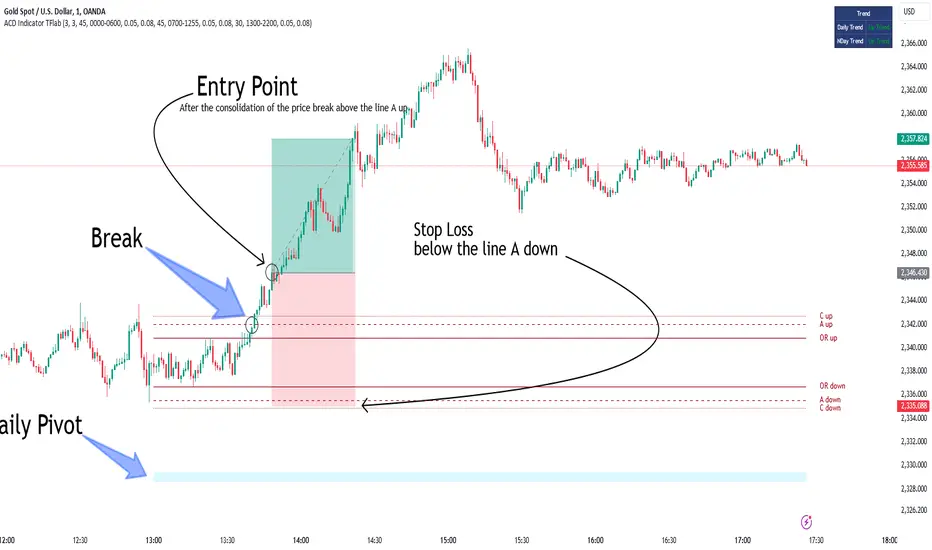
Ichimoku Breakout Kumo SWING TRADER (By Insert Cheese)A simple strategy for long spot or long futures (swing traders) based on a basic method of Ichimoku Kinko Hyo strategies.
The strategy is simple:
- Buy when the price breaks the cloud
- Close the trade when the price closes again inside the cloud.
The parameters that work best on this strategy are 10,30,60,30 and 1 for Senkou-Span A
but you can try classic Ichimoku parameters (9,26,52,26,26) or whatever you want like (7,22,44,22,22), (10,30,60,30,30) and others.
-1D chart
I have removed everything from the interface except the cloud to make it visually more aesthetic :D (but if you want to see all the ichimoku indicator you can put in again into the chart)
I have also added several functions for you to do your own backtesting:
- Date range
- TP AND SL method
- Includes long or short trades
The strategy starts with 500 $ and use 100% for trade to make the power of the compounding :P
Remember that this is for only educational porpouse and you must to do your own research and backtested on your usually market..
I hope you like it enjoy and support this indicator :)
Donate (BEP20) 0xC118f1ffB3ac40875C13B3823C182eA2Af344c6d
Ranged Volume DCA Strategy - R3c0nTraderUpdate: Republishing this as Public Open-Source script.
Credits:
Thank you "EvoCrypto" for granting me permission to use "Ranged Volume" to create this strategy.
Thank you "junyou0424" for granting me permission to use "DCA Bot with SuperTrend Emulator" which I used for adding bot inputs, calculations, and strategy
What does this do?
This script is mainly used for backtesting a Ranged Volume strategy to see how a 3Commas bot would perform.
I created this script out of necessity and I wanted a way to test a 3Commas DCA bot with a strategy based on “Volume.”
I came across "EvoCrypto’s" "Ranged Volume" study and strategy in TradingView and I liked it. I wanted to configure it so it can be used for DCA bot backtesting. I used parts from "junyou0424’s" "DCA Bot with SuperTrend Emulator" to add the following:
1. The Start Time and End Time
2. Price deviation to open safety orders (%)
3. Target Take Profit (%)
4. Trailing deviation
5. Base Order and Safety Order
6. Safety order volume scale
7. Safety order step scale
8. Max safety orders
In addition to the above, I also added chart indicators for "Take Profit" as well as "Safety Order"
Pre-requisites:
You can use this script without a 3Commas account and see how 3Commas DCA Bot and Ranged Volume strategy would perform vs. a non-DCA strategy. However, I highly recommend signing up for their free account and going through their training. This would give you a base understanding on the settings you will see in this strategy and why you will need to know them.
That said these are the pre-requisites I suggest you have:
1. Base Knowledge of 3Commas DCA bots
2. Base knowledge of settings such as “Max safety trades count”, “safety order volume scale” and “safety order step scale”. If these are alien to you, I suggest you read up on these.
3. Knowledge of setting up a Single-pair 3Commas bot for receiving custom TradingView signal.
4. A paper-bot to test your ideas. (Do not use a real money bot until you have tested it sufficiently with a paper-bot. You alone are responsible for your results!)
5. Add the study I created called "R3c0nTrader’s Ranged Volume Study” which adds a separate chart in its own pane showing the volume spikes. It will also generate the “buy” signals for your bot. NOTE: The study also has the same color scheme as this strategy and having the colors in both the strategy and the study will make things easier to see. If you use EvoCrypto’s Ranged Volume Study instead, just keep in mind that the colors won’t match, and you will have to manually match them.
6. Make your buy signals from your strategy are the same as in your study! To do this, use the same “Volume Range Length” you entered in the STRATEGY and enter that value for the “Volume Range Length” in the STUDY. Also ensure you have the same settings for “Heikin Ashi” (On or Off).
Comparisons of Ranged Volume Strategy vs Ranged Volume DCA Strategy
BTCUSD
Beware of Strategies that claim super high profits. This can easily be done by lowering the initial capital to something unrealistic. If I did that with this strategy and set the initial capital $100 and base order size to $100, I get a net profit of 2,864% which is not realistic.
How to Use
1. On the “Inputs” tab:
a. Set your Start and End Time to backtest against.
b. Set your “Volume Range Length” (number of bars to look back)
c. “Heikin Ashi Colors” – Usually I leave this enabled
d. “Show Bar Colors” – Leave enabled
e. “Show Break-Out” – Leave enabled
f. “Show Range” – Leave enabled
g. Set your other inputs which are those settings you would find in your 3Commas bot that you want to test (e.g., Price deviation to open safety orders, Target Take Profit, Base order, Safety order, etc.).
h. Quick Example for BTCUSD on 2hr chart:
i. Price deviation to open safety orders (%) = 6
ii. Target Take Profit (%) = 14
iii. Trailing deviation = 0
iv. Base order = 100
v. Safety order = 200
vi. Safety order volume scale = 2
vii. Safety order step scale = 1.4
viii. Max safety order = 5
2. On the “Properties” tab, set your initial capital, base currency, etc.
a. Initial capital – Default is 10,000 (Please use realistic values here. The amount here should be able to cover ALL your safety orders if they were triggered. Ideally, you should have funds left over and not use all trade capital.)
b. Base currency – Select your currency
c. Order Size - Not used. Use the “Inputs” tab to change your base order size.
d. Leave “Pyramiding” set to 999. This acts as a ceiling to the “Max safety orders” on the “Inputs” tab. It must always be higher than your “Max safety orders.” For example, if you set your “Max safety orders” to “4” and “Pyramiding” to “4” then it effectively means you have “3” “Max safety orders” and not “4” because it is counting each successive entry including the initial order.
e. “Commission” - Optional
f. “Verify price for limit orders” – Leave at zero. This does not change anything that I can tell.
g. Optional - Enter a value for “Commission”
h. Slippage – Optional. Slippage does not occur in backtesting but does occur in real trading but it can be simulated. Example use case for tracking performance of a real money bot: You enter the start date and time of your bot’s trade into this strategy and you notice some values are a little off due to slippage (average price, take profit, safety orders are not lining up) then you would go back here and increase the slippage until those lines up close enough with your actuals.
i. Margin for long positions – I don’t use this honestly.
j. Margin for short positions – I don’t use this honestly.
k. Recalculate “After order is filled” and “On every tick” – I don’t use this honestly.
3. “Style” tab
a. Ranged Volume Bar Coloring - You must disable bar coloring in any studies you added or this may not work properly
i. Color 0 – Default Yellow; appears when a volume breakout occurs
ii. Color 1 – Default Red; appears when a volume breakdown occurs
iii. Color 2 – Light Blue; appears when Close is higher than the Open
iv. Color 3 – Dark Blue; appears when the Close is lower than the Open
b. Take profit – Default Green; take profit line
c. Safety order – Default Light Blue; safety order line
d. No Safety Orders left – Default Red; when a trade runs out of safety orders, the line turns red and there is no safety orders left underneath to catch any further falling price movements.
e. Avg Position Price – Default Orange; your average position price for any given trade.
f. Take Profit Plot Area – Default Green; creates a highlighted area for your take profit
g. SO Plot Area – Default Light Blue; creates a highlighted area for your safety orders
h. Trades on chart – Show or hide your trades on the chart
i. Signal labels – Show or hide the trade signal labels on the chart
j. Quantity – Show or hide the trade quantity on the chart
Explanation of Chart lines and colors on chart

Ichimoku Cloud Strategy Long Only [Bitduke]Slightly modificated and optimized for Pine Script 4.0, Ichimoku Cloud Strategy which, suddenly, good suitable for the several crypto assets.
Details:
Enter position when conversion line crosses base line up, and close it when the opposite happens.
Additional condition for open / close the trade is lagging span, it should be higher than cloud to open position and below - to close it.
Backtesting:
Backtested on SOLUSDT ( FTX, Binance )
+150% for 2021 year, 8% dd
+191% for all time, 32% dd
Disadvantages:
- Small number of trades
- Need to vary parameters for different coins (not very robust)
Should be tested carefully for other coins / stock market. Different parameters could be needed or even algo modifications.
Strategy doesn't repaint.
Support BandsSupport Bands – Discount Zones for Bitcoin
⚡Overview:
-The Support Bands indicator identifies one of the most tested and respected support zones for Bitcoin using moving averages from higher timeframes.
-These zones are visualized through colored bands (blue, white, and violet), simplifying the decision making process especially for less experienced traders who seek high-probability areas to accumulate Bitcoin during retracements.
-Band levels are based on manual backtesting and real-world price behavior throughout Bitcoin’s history.
-Each zone reflects a different degree of support strength, from temporary pullback zones to historical bottoms.
⚡️ Key Characteristics:
-Highlights discount zones where Bitcoin has historically shown strong reactions.
-Uses 3 different levels of supports based on EMA/SMA combinations.
-Offers a clean, non-intrusive overlay that reduces chart clutter.
⚡ How to Use:
-Open your chart on the 1W timeframe and select the BTC Bitstamp or BLX symbol, as they provide the most complete historical data, ensuring optimal performance of the indicator.
-Use the bands as reference zones for support and potential pullbacks.
- Level 3 (violet band) historically marks the bottom of Bitcoin bear markets and is ideal for long-term entries during deep corrections.
- Level 2 (white band) often signals macro reaccumulation zones but usually requires 1–3 months of consolidation before a breakout. If the price closes below and then retests this level as resistance for 1–2 weekly candles, it often marks the start of a macro downtrend.
-Level 1 (blue band) acts as short-term support during strong bullish moves, typically after a successful rebound from Level 2.
⚡ What Makes It Unique:
- This script merges moving averages per level into three simplified bands for clearer analysis.
-Reduces chart noise by avoiding multiple overlapping lines, helping you make faster and cleaner decisions.
- Built from manual market study based on recurring Bitcoin behavior, not just random code.
-Historically backtested:
-Level 3 (violet band) until today has always marked the bitcoin bearmarket bottom.
- Level 2 (white band) is the strongest support during bull markets; losing it often signals a macro trend reversal.
- Level 1 is frequently retested during impulsive rallies and can act as short-term support or resistance.
⚡ Disclaimer:
-This script is a visual tool to assist with market analysis.
-It does not generate buy or sell signals, nor does it predict future movements.
-Historical performance is not indicative of future results.
-Always use independent judgment and proper risk management.
⚡ Why Use Support Bands:
-Ideal for traders who want clarity without dozens of lines on their charts.
- Helps identify logical zones for entry or reaccumulation.
- Based on actual market behavior rather than hypothetical setups.
-If the blue band (Level 1) doesn't hold as support, the price often moves to the white band (Level 2), and if that fails too, the violet band (Level 3) is typically the last strong support. By dividing your capital into three planned entries, one at each level,you can manage risk more effectively compared to entering blindly without this structure.