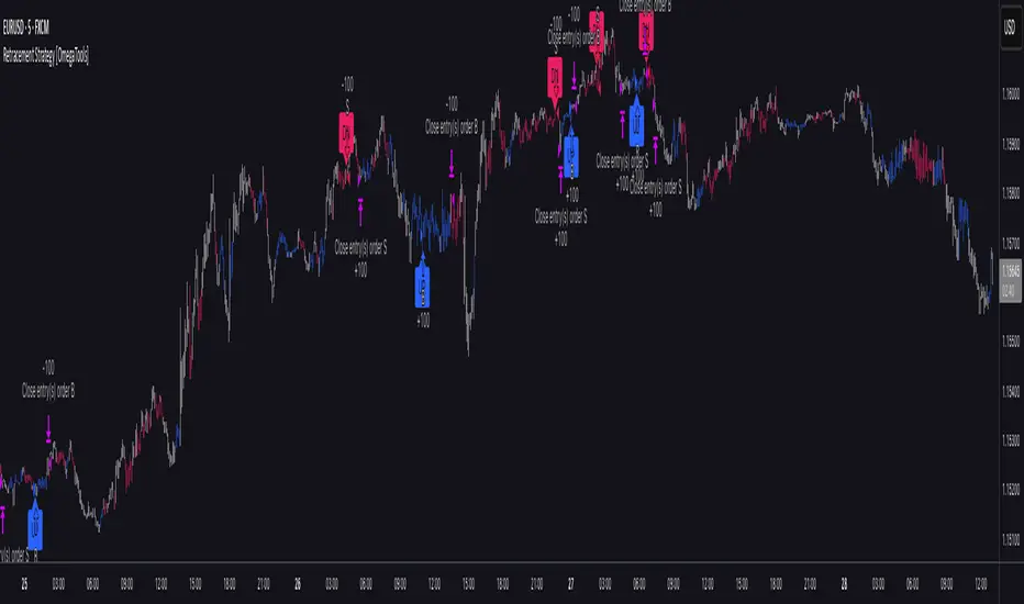
Retracement Strategy [OmegaTools]Retracement Strategy is a systematic trend–retracement framework designed to identify directional opportunities after a confirmed momentum shift, and to manage exits using either trend reversals or overextension conditions. It is built around a smoothed RSI regime filter and a simple, price-based retracement trigger, making it applicable across a wide range of markets and timeframes while remaining transparent and easy to interpret.
The strategy begins by defining the underlying trend through a two-stage RSI signal. A standard RSI is computed over the user-defined Length input, then smoothed with a short moving average to reduce noise. Two symmetric thresholds are derived from the Threshold parameter: an upper band at 100 minus the threshold and a lower band at the threshold itself. When the smoothed RSI crosses above the upper band, the environment is classified as bullish and the internal trend state is set to uptrend. When the smoothed RSI crosses below the lower band, the environment is classified as bearish and the trend state becomes downtrend. When RSI moves back into the central zone between the two bands, the trend is considered neutral. In addition to the current trend, the strategy tracks the last non-neutral trend direction, which is used to detect genuine trend changes rather than transient oscillations.
Once a trend is established, the strategy looks for retracement entries in the direction of that trend. For long setups in an uptrend, it computes the lowest low over the previous Length minus one bars, excluding the current bar. A long signal is generated when price dips below this recent low while the trend state remains bullish. Symmetrically, for short setups in a downtrend, it computes the highest high over the previous Length minus one bars and enters short when price spikes above this recent high while the trend state remains bearish. This logic is designed to capture pullbacks against the prevailing RSI-defined trend, entering when the market tests or slightly violates recent extremes, rather than chasing breakouts. The candles are visually coloured to reflect the detected trend, highlighting bullish and bearish environments while keeping neutral phases distinguishable on the chart. An ATR-based measure is used solely to position the “UP” and “DN” labels on the chart for clearer visualisation of entry points; it does not directly influence position sizing or stop calculation in this implementation.
Take profit and stop loss behaviour are fully parameterized through the “Take Profit” and “Stop Loss” inputs, each offering three modes: None, Trend Change and Extension. When “Trend Change” is selected for the take profit, the strategy will only exit profitable positions when a confirmed trend reversal occurs. For a long position, this means that the strategy will close the trade when the trend state flips from uptrend to downtrend, and the last recorded trend direction validates that this is a genuine reversal rather than a neutral fluctuation; the same logic applies symmetrically for short positions. When “Extension” is selected as the take profit mode, the strategy closes profitable long trades when the smoothed RSI reaches or exceeds the upper threshold, interpreted as an overbought extension within the bullish regime, and closes profitable short trades when the smoothed RSI falls to or below the lower threshold, interpreted as an oversold extension within the bearish regime. When “None” is chosen, the strategy does not apply any explicit take profit logic, leaving trades to be managed by the stop loss settings or by user discretion in backtesting.
The stop loss parameter works in a parallel way. With “Trend Change” selected as stop loss, any open long position is closed when the trend flips from uptrend to downtrend, regardless of whether the trade is currently in profit or loss, and any open short is closed when the trend flips from downtrend to uptrend. This turns the RSI trend regime into a hard invalidation rule: once the underlying momentum structure reverses, the position is exited. With “Extension” selected for stop loss, long positions are closed when RSI falls back below the upper band and moves towards the opposite side of the range, while short positions are closed when RSI rises above the lower band and moves towards the upper side. In practice, this acts as a dynamic exit based on the oscillator moving out of a favourable context for the existing trade. Selecting “None” for stop loss disables these automatic exits, leaving only the take profit logic, if any, to manage the position. Because take profit and stop loss configuration are independent, the user can construct different profiles, such as pure trend-change exits on both sides, pure overextension exits, or a mix (for example, take profit on overextension and stop loss on trend reversal).
This strategy is designed as an analytical and backtesting framework rather than a finished plug-and-play trading system. It does not include position sizing, risk-per-trade controls, multi-timeframe confirmation, volatility filters or instrument-specific fine-tuning. Its primary purpose is to provide a clear, rule-based structure for testing retracement logic within RSI-defined trends, and to allow users to explore how different exit regimes (trend-change based versus extension based) affect performance on their instruments and timeframes of interest.
Nothing in this script or its description should be interpreted as financial advice, investment recommendation or solicitation to buy or sell any financial instrument. Past performance on backtests does not guarantee future results. The behaviour of this strategy can vary significantly across symbols, timeframes and market conditions, and correlations, volatility and liquidity can change without warning. Before considering any live application, users should thoroughly backtest and forward test the strategy on their own data, adjust parameters to their risk profile and instrument characteristics, and integrate proper money management and trade management rules. Use of this script is entirely at the user’s own risk.
Cerca negli script per "backtest"
2-Period RSI strategy (with filter)2-period RSI strategy backtest described in several books of the trader Larry Connors . This strategy uses a 2 periods RSI , one slow arithmetic moving average and one fast arithmetic moving average.
Entry signal:
- RSI 2 value below oversold level (Larry Connors usually sets oversold to be below 5, but other authors prefer to work below 10 due to the higher number of signals).
- Closing above the slow average (200 periods).
- Entry at closing of candle or opening of next candle.
Exit signal:
- Occurs when the candlestick closes above the fast average (the most common fast average is 5 periods, but some traders also suggest the 10 period average).
Entry Filter (modification made by me):
- Applied an RSI2 arithmetic moving average to smooth out oscillations.
- Entered only when RSI2 is below oversold level and RSI2 moving average is below 30.
* NOTE: In the stocks that I evaluate daily the averages of 4 and 6 periods work very well as a filter.
Comments:
This strategy works very well in Daily charts but can be applied in other chart times as well. As this is a strategy to catch market fluctuations, it presents different results with different stocks.
I have been applying this strategy to the stocks of the Brazilian market (BOVESPA) and have enjoyed the result. Every day I evaluate the stocks that are generating entry signals and choose which one to trade based on the stocks with the highest Profit Value.
The RSI 2 averaging filter probably will reduce profit of the backtests because reduces the number of signals, but the Profit Value will usually increase. For me this was a good thing because without the filter, this strategy usually shows more signals than I have capital to allocate.
Before entering a trade I look at which fast average the paper has the highest Profit Value and then I use this average as my output signal for that trade (this change has greatly improved the result of the outputs).
This strategy does not use Stop Loss because normally Stop Loss decreases effectiveness (profit). In any case, the option to apply a percentage Stop Loss if desired is added in the script. As the strategy does not use stop, extra caution with risk management is advisable. I advise not to allocate more than 20% of the trade capital in the same operation.
I'm still studying ways to improve this strategy, but so far this is the best setup I've found. Suggestions are always welcome and we can test to see if they improve the backtest result.
Good luck and good trades.
================================================
Backtest das estratégia do IFR de 2 períodos descrita em varios livros do trader Larry Connors . Esta estratégia usa um IFR de 2 períodos, uma média movel aritmética lenta e uma média movel aritmética rápida.
Sinal de entrada:
- Valor do IFR 2 abaixo do nível de sobrevenda (Larry Connors usualmente define sobrevenda sendo abaixo de 5, mas outros autores preferem trabalhar abaixo de 10 devido ao maior número de sinais).
- Fechamento acima da média lenta (200 períodos).
- Realizado a compra no fechamento do candle ou na abertura do candle seguinte.
Sinal de saída:
- Ocorre quando o candle fecha acima da média rápida (a média rápida mais comum é a de 5 períodos, mas alguns traders sugerem também a média de 10 períodos).
Filtro para entrada (modificação feita por mim):
- Aplicado uma média móvel aritmética do IFR2 para suavisar as oscilações.
- Realizado a entrada apenas quando o IFR2 está abaixo do nível de sobrevenda e a média móvel do IFR2 está abaixo de 30.
*OBS: nos ativos que avalio diariamente as médias de 4 e 6 períodos funcionam muito bem como filtro.
Comentários:
Esta estratégia funciona muito bem no tempo gráfico Diário mas pode ser aplicada tambem em outros tempos gráficos. Como trata-se de uma estratégia para pegar oscilações do mercado, ela apresenta diferentes resultados com diferentes ativos.
Eu venho aplicando esta estratégia nos ativos do mercado brasileiro (BOVESPA) e tenho gostado do resultado. Diariamente eu avalio os papeis que estão gerando entrada e escolho qual irei realizar o trade baseado nos papeis que apresentam maior Profit Value.
O filtro da média do IFR 2 reduz o lucro nos backtests pois reduz também a quantidade de sinais, mas em compensação o Profit Value irá normalmente aumentar. Para mim isto foi algo positivo pois, sem o filtro, normalmente esta estratégia apresenta mais sinais do que possuo capital para alocar.
Antes de entrar em um trade eu olho em qual média rápida o papel apresenta maior Profit Value e então eu utilizo está média como meu sinal de saída para aquele trade (esta mudança tem melhorado bastante o resultado das saídas).
Está estratégia não utiliza Stop Loss pois normalmente o Stop Loss diminui a eficácia (lucro). De qualquer maneira, foi acrescentado no script a opção de aplicar um Stop Loss percentual caso seja desejado. Como a estratégia não utiliza stop é aconselhável um cuidado redobrado com o gerenciamento de risco. Eu aconselho não alocar mais de 20% do capital de trade em uma mesma operação.
Ainda estou estudando formas de melhorar esta estratégia, mas até o momento está é a melhor configuração que encontrei. Sugestões são sempre bem vindas e podemos testar para verificar se melhoram o resultado do backtest.
Boa sorte e bons trades.

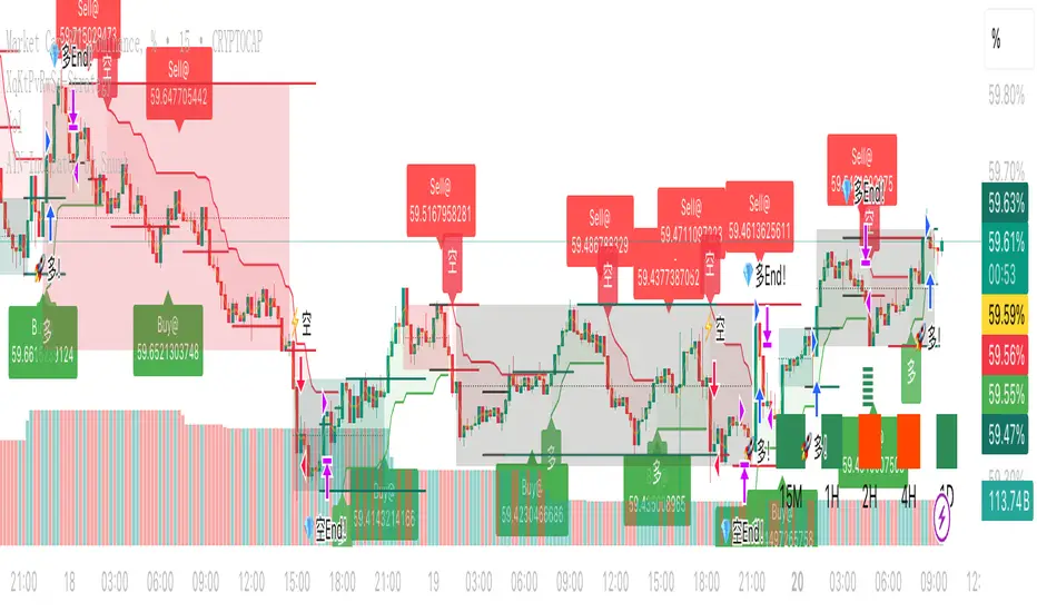
XqKtPvRwSd-StrategyTradingView Pine Script Suite (v4.0) — General Overview
Purpose
A modular indicator and strategy suite designed for crypto markets, focusing on trend detection, momentum, range visualization, and signal generation. The suite supports popular symbols (BTC, ETH, BNB, SOL, DOGE) and offers flexible visualization and alert options.
Main Components
- v4.0-indicator: Multi-signal display for monitoring market conditions and trend bias.
- v4.0-watch-15m: Watchlist-style indicator with symbol-aware auto-tuning and optional chart timeframe adaptation.
- v4.0-strategy: Backtestable strategy using a unified, SuperTrend-based trend determination for entries/exits.
- v4.0-range: Range and structure visualization with dynamic lines, zones, and basic breakout cues.
- Two Poles.pinescript and fengzi/Two Poles Trend: Low-lag trend and smoothing filters for stability.
- supertrend.pinescript: SuperTrend variations used across the suite for direction and stops.
- fengzi utilities:
- Hann Window FIR Filter: Denoising and smoothing to reduce noise without excessive lag.
- Heatmap + Hann Resonance: Visual heat/energy mapping for momentum and resonance cues.
- Heatmap Trailing Stop with Breakouts: Trailing stop framework with breakout detection.
- Additional modules: super Z, AI JX, v3.2, and 4.0.pinescript (combined or experimental entries).
Key Features
- Unified Trend Logic: Strategy and visual components rely on a consistent SuperTrend-based direction model, improving clarity and consistency.
- Adaptive Timeframe: Option to use the chart’s timeframe; parameters scale from a 15m baseline to maintain relative behavior.
- Symbol Auto-Tuning: Default parameter sets are tailored for common crypto symbols; manual overrides are available.
- RSI Top/Bottom Hints: Optional dynamic cues for potential peaks in uptrends and troughs in downtrends; can contribute to scoring and alerts.
- Visual Customization: Configurable markers (arrows, dots, crosses), colors, line widths, and subtle background highlighting.
- Scoring and Clustering: Combines checks into a simplified score and clusters signals to reduce noise.
- Alerts: Supports TradingView alerts for entries, exits, and RSI hints.
- Compatibility: Designed to compile across common Pine versions and avoid local-scope plotting issues.
Basic Usage
- Add the indicator or strategy to your chart depending on your goal (monitoring vs. backtesting).
- Choose to follow the chart’s timeframe or set a working timeframe manually.
- Keep symbol auto-tuning enabled for a balanced default, or adjust parameters to match your preferences.
- Toggle optional modules (RSI hints, scoring contribution, visualization) based on your needs.
- For strategies, run backtests across your target period and review performance metrics (win rate, drawdown, and trade frequency).
Configuration Guidelines
- For earlier entries: lower SuperTrend period or multiplier; relax RSI thresholds.
- For more conservative behavior: increase SuperTrend period or multiplier; tighten thresholds; use stricter RSI logic.
- For cleaner signals: rely on the unified trend and consider limiting trades during extreme volatility or illiquid sessions.
Outputs
- Trend markers and lines indicating bullish/bearish bias and reversals.
- Range drawings with dynamic line coordinates, zones, and visual cues for consolidations and breakouts.
- Optional multi-timeframe dashboard-style summaries where applicable.
Extensibility
- Parameters and defaults can be extended for additional symbols and styles.
- Optional weighting or neutrality rules can be added to trend logic if you prefer stricter confirmation.
- Additional filters (volatility, session, volume) can be integrated to refine entries and exits.
Notes
- Not financial advice; backtest thoroughly before using any strategy live.
- Performance and signal quality vary by symbol, timeframe, and market conditions; adjust parameters as needed.
- Pine version differences may require minor adjustments; keep your environment up to date.
Baseline TrendBaseline Trend Strategy Overview
Baseline Trend is a crypto-only trading strategy built on straightforward price-based logic: market direction is determined solely by the price’s position relative to a selected baseline open price. No technical indicators like RSI, MACD, or volume are used—this approach is purely focused on price action and position size manipulation.
This strategy is a genuine concept, developed from my own market analysis and logical theory, refined through extensive observation of crypto market behaviour.
While the strategy offers structure and adaptability, it’s important to recognise that no single trading system or indicator fits all market conditions. This tool is meant to support decision-making, not replace it—encouraging traders to stay flexible, informed, and in control of their risk.
Important Usage Note:
This system is intended for crypto markets only.
– When used as an indicator guide, it can be applied to both spot and futures markets.
– However, when used with web-hook automation, it is designed only for futures contracts.
Ensure compatibility with your trading setup before using automation features.
Core Logic: The Baseline
The strategy revolves around the concept of a “Baseline”, with three types available:
Main Baseline: Defines the primary trend direction. If the price is above, go long; if below, go short.
Second Baseline and Third Baseline: Used to measure buying/selling pressure and are key to certain take-profit logic options.
Baselines are customisable to different timeframes—Year, Month, Week, and more—based on available input settings. Structurally, the Main Baseline is the highest-level trend reference, followed by the Second, then Third.
Users can mix and match these baselines across timeframes to backtest crypto symbols and understand behaviour patterns, particularly when used with standard candlestick charts.
Entry & Exit Logic
Entry Signal: Triggered when price crosses over/under a defined distance (percentage) from the Main Baseline. This distance is the Trade Line, calculated based on the close price.
Exit Signal / Stop Loss: If price moves un-favorable and crosses over/under the Stop Loss Line (a defined distance from the Main Baseline), the open position will be force-closed according to user-defined settings.
LiqC (Liquidation Cut)
LiqC is a secondary stop-loss that activates when a leveraged position’s loss equals or exceeds the user-defined liquidation threshold. It forcefully closes the position to help prevent full liquidation before stop-loss, providing an extra layer of protection.
This LiqC is directly tied to the leverage level set by the user. Please ensure you understand how leverage affects liquidation risk, as different broker exchanges may use different liquidation ratio models. Using incorrect assumptions or mismatched leverage values may result in unexpected behaviour.
Position Sizing & Block Units
This strategy features a block-based position sizing system designed for flexibility and precision in trade management:
Block Range: Customisable from 1 to 10 blocks
Risk Allocation: Controlled through a user-defined ROE (Risk of Equity) value
For example, setting an ROE of 0.1% with 10 blocks allocates a total of 1% of account equity to the position. This structure supports both conservative and aggressive risk approaches, depending on user preference.
Block sizes are automatically calculated in alignment with exchange requirements, using Minimum Notional Value (MNV) and Minimum Trade Amount (MTA). These values are dynamically calculated based on the live market price, and scaled relative to the trader’s balance and selected risk percentage. This ensures accurate sizing with built-in adaptability for any account level and current market conditions.
Scalping Meets Trend Holding
This system blends short-term scalping with longer-term trend holding, offering a flexible and adaptive trading style.
Example:
Enter 10 blocks → take quick profits on 5 blocks → let the remaining 5 ride the trend.
This dual-layered approach allows traders to secure early gains while staying positioned for larger market moves. Think of it as:
5 Blocks to Protect: Capture quick wins and manage exposure.
5 Blocks to Pursue: Let profits run by following the broader trend.
By combining both protection and pursuit, the strategy supports risk control without sacrificing the potential for extended returns.
Flexible Take-Profit Logic
The strategy supports multiple, customisable take-profit mechanisms:
TP1–4 (Profit Percentage)
Triggers take profit of 1 block unit when unrealised gains reach defined percentage thresholds (TP1, TP2, TP3, TP4).
Buying/Selling Pressure-Based Take Profit
D1 – Pressure 1
Measures pressure between Second and Third Baselines.
If the distance between them exceeds a user-defined DPT (Decrease Post Threshold) and the price moves far enough from the Third Baseline, D1 activates to take profit or scale out one block.
D2 – Pressure 2
Measures pressure between the Main and Second Baselines.
Works similarly to D1, using a separate distance and pressure trigger.
Note: Both D1 and D2 deactivate in reversal or even trend conditions.
D3–5: High-High / Low-Low Logic
Based on bar index tracking after position entry:
For Long Positions: If after D3 bars the price doesn't exceed the previous bar's high, the system executes a take profit or scale-out.
For Short Positions: If the price doesn't drop below the previous low, the same logic applies.
This approach adds time-based and momentum-aware exit flexibility.
Leverage & Liquidation Risk
When backtesting with leverage enabled, the system checks whether historical candles exceed the liquidation range, calculated based on the average entry price and the leverage input. If the Liquidation Risk Count exceeds 1, profit and loss accuracy may be affected. Traders are encouraged to monitor this count closely to ensure realistic backtesting results.
Since the system cannot directly control or sync with your broker exchange’s actual leverage setting, it’s important to manually match the system’s leverage input with your broker’s configured leverage.
For example: If the system leverage input is set to 10, your exchange leverage setting must also be set to 10. Any mismatch will lead to inaccurate liquidation risk and PnL calculations.
Backtesting and Customisation
All TP1–4 and D1–5 functions are fully optional and customisable. Users are encouraged to backtest different crypto symbols to observe how price behaviour aligns with baseline structures and pressure metrics.
Each of the TP1–4 and D1–5 triggers is designed to execute only once per open position, ensuring controlled and predictable behaviour within each trade cycle.
Since backtesting is based on available historical bar data, please note that data availability varies depending on your TradingView subscription plan. For more reliable insights, it’s recommended to backtest across multiple time ranges, not just the full dataset, to assess the stability and consistency of the strategy’s performance over time.
Additionally, the time frame resolution interval in TradingView is customisable. For best results, use commonly supported time frames such as 30 minutes, 1 hour, 4 hours, 1 day, or 1 week. While the system is designed to support a broad range of intervals, non-standard resolutions may still cause calculation errors.
Currently, the system supports the following resolution ranges:
Intraday: from 1 minute to 720 minutes
(e.g., 60 minutes = 1 hour, 240 minutes = 4 hours, 720 minutes = 12 hours)
Daily: from 1 day to 6 days
Weekly: from 1 week to 3 weeks
Monthly: from 1 month to 4 months
Although the script is built to adapt to various resolutions, users should still monitor output behaviour closely, especially when testing less common or edge-case time frames.
System Usage Notice:
This system can be used as a standalone trading indicator or integrated with an exchange that supports web-hook signal execution. If you choose to automate trades via web-hook, please ensure you fully understand how to configure the setup properly. Web-hook integration methods vary between exchanges, and incorrect setup may lead to unintended trades. Users are responsible for ensuring proper configuration and monitoring of their automation.
Note on Lower Time Frame Usage
When using lower time frames (e.g., 1-minute charts) as the trading time frame, please be aware that available historical data may be limited depending on your subscription plan. This can affect the depth and reliability of backtesting, making it harder to establish a trustworthy probability model for a symbol’s behaviour over time.
Additionally, when pairing a high-level Main Baseline (MBL) time line (such as "1 Month") with low time frame resolutions (like 1-minute), you may encounter order execution limits or calculation overloads during backtesting. This is due to the large number of historical bars required, which can strain the system's capacity.
That said, if a user intentionally chooses to work with lower time frames, that decision is fully respected—but it should be done with awareness and at the user’s own risk.
Things to Be Aware Of (Web-hook Usage Only)
The following points apply if you're using web-hook automation to send signals from the system to an exchange:
Alert Signal Reliability
During extreme market volatility, some broker exchanges may fail to respond to web-hook signals due to traffic overload. While rare, this has occurred in the past and should be considered when relying on automation.
Alert Expiration (TradingView)
If you're on a Basic plan, TradingView alerts are only active for a limited time—typically around 1.5 months. Once expired, signals will no longer be sent out.
To keep your system active, reset the alert before expiration. For uninterrupted alerts, consider upgrading to a Premium plan, which supports permanent alert activation.
TradingView Alert Maintenance
TradingView may occasionally perform system maintenance, during which alerts may temporarily stop functioning. It’s recommended to monitor TradingView’s status if you’re relying on real-time automation.
Repainting
As of the current version, no repainting behaviour has been observed. Signal stability and consistency have been maintained across real-time and historical bars.
Order Execution Type and Fill Logic
All signals use Limit orders by default, except for MBL Exit and Fallback execution, which use Market orders.
Since Limit orders are not guaranteed to fill, the system includes logic to cancel unfilled orders and resend them. If necessary, a Fallback Market order is used to avoid conflict with new incoming trades.
This has only happened once, and is considered rare, but users should always monitor execution status to ensure accuracy and alignment with system behaviour.
Feedback
If you encounter any errors, bugs, or unexpected behaviour while using the system, please don’t hesitate to let me know. Your input is invaluable for helping improve the strategy in future updates.
Likewise, if you have any suggestions or ideas for enhancing the system—whether it’s a new feature, adjustment, or usability improvement—please feel free to share. Together, we can continue refining the tool to make it more robust and beneficial for everyone.
Disclaimer
All trading involves risk, particularly in the crypto market where conditions can be highly volatile. Past performance does not guarantee future outcomes, and market behaviour may evolve over time. This strategy is offered as a tool to support trading decisions and should not be considered financial or investment advice. Each user is responsible for their own actions and accepts full responsibility for any results that may arise from using this system.

Bitcoin 5A Strategy@LilibtcIn our long-term strategy, we have deeply explored the key factors influencing the price of Bitcoin. By precisely calculating the correlation between these factors and the price of Bitcoin, we found that they are closely linked to the value of Bitcoin. To more effectively predict the fair price of Bitcoin, we have built a predictive model and adjusted our investment strategy accordingly based on this model. In practice, the prediction results of this model correspond quite high with actual values, fully demonstrating its reliability in predicting price fluctuations.
When the future is uncertain and the outlook is unclear, people often choose to hold back and avoid risks, or even abandon their original plans. However, the prediction of Bitcoin is full of challenges, but we have taken the first step in exploring.
Table of contents:
Usage Guide
Step 1: Identify the factors that have the greatest impact on Bitcoin price
Step 2: Build a Bitcoin price prediction model
Step 3: Find indicators for warning of bear market bottoms and bull market tops
Step 4: Predict Bitcoin Price in 2025
Step 5: Develop a Bitcoin 5A strategy
Step 6: Verify the performance of the Bitcoin 5A strategy
Usage Restrictions
🦮Usage Guide:
1. On the main interface, modify the code, find the BTCUSD trading pair, and select the BITSTAMP exchange for trading.
2. Set the time period to the daily chart.
3. Select a logarithmic chart in the chart type to better identify price trends.
4. In the strategy settings, adjust the options according to personal needs, including language, display indicators, display strategies, display performance, display optimizations, sell alerts, buy prompts, opening days, backtesting start year, backtesting start month, and backtesting start date.
🏃Step 1: Identify the factors that have the greatest impact on Bitcoin price
📖Correlation Coefficient: A mathematical concept for measuring influence
In order to predict the price trend of Bitcoin, we need to delve into the factors that have the greatest impact on its price. These factors or variables can be expressed in mathematical or statistical correlation coefficients. The correlation coefficient is an indicator of the degree of association between two variables, ranging from -1 to 1. A value of 1 indicates a perfect positive correlation, while a value of -1 indicates a perfect negative correlation.
For example, if the price of corn rises, the price of live pigs usually rises accordingly, because corn is the main feed source for pig breeding. In this case, the correlation coefficient between corn and live pig prices is approximately 0.3. This means that corn is a factor affecting the price of live pigs. On the other hand, if a shooter's performance improves while another shooter's performance deteriorates due to increased psychological pressure, we can say that the former is a factor affecting the latter's performance.
Therefore, in order to identify the factors that have the greatest impact on the price of Bitcoin, we need to find the factors with the highest correlation coefficients with the price of Bitcoin. If, through the analysis of the correlation between the price of Bitcoin and the data on the chain, we find that a certain data factor on the chain has the highest correlation coefficient with the price of Bitcoin, then this data factor on the chain can be identified as the factor that has the greatest impact on the price of Bitcoin. Through calculation, we found that the 🔵number of Bitcoin blocks is one of the factors that has the greatest impact on the price of Bitcoin. From historical data, it can be clearly seen that the growth rate of the 🔵number of Bitcoin blocks is basically consistent with the movement direction of the price of Bitcoin. By analyzing the past ten years of data, we obtained a daily correlation coefficient of 0.93 between the number of Bitcoin blocks and the price of Bitcoin.
🏃Step 2: Build a Bitcoin price prediction model
📖Predictive Model: What formula is used to predict the price of Bitcoin?
Among various prediction models, the linear function is the preferred model due to its high accuracy. Take the standard weight as an example, its linear function graph is a straight line, which is why we choose the linear function model. However, the growth rate of the price of Bitcoin and the number of blocks is extremely fast, which does not conform to the characteristics of the linear function. Therefore, in order to make them more in line with the characteristics of the linear function, we first take the logarithm of both. By observing the logarithmic graph of the price of Bitcoin and the number of blocks, we can find that after the logarithm transformation, the two are more in line with the characteristics of the linear function. Based on this feature, we choose the linear regression model to establish the prediction model.
From the graph below, we can see that the actual red and green K-line fluctuates around the predicted blue and 🟢green line. These predicted values are based on fundamental factors of Bitcoin, which support its value and reflect its reasonable value. This picture is consistent with the theory proposed by Marx in "Das Kapital" that "prices fluctuate around values."
The predicted logarithm of the market cap of Bitcoin is calculated through the model. The specific calculation formula of the Bitcoin price prediction value is as follows:
btc_predicted_marketcap = math.exp(btc_predicted_marketcap_log)
btc_predicted_price = btc_predicted_marketcap / btc_supply
🏃Step 3: Find indicators for early warning of bear market bottoms and bull market tops
📖Warning Indicator: How to Determine Whether the Bitcoin Price has Reached the Bear Market Bottom or the Bull Market Top?
By observing the Bitcoin price logarithmic prediction chart mentioned above, we notice that the actual price often falls below the predicted value at the bottom of a bear market; during the peak of a bull market, the actual price exceeds the predicted price. This pattern indicates that the deviation between the actual price and the predicted price can serve as an early warning signal. When the 🔴 Bitcoin price deviation is very low, as shown by the chart with 🟩green background, it usually means that we are at the bottom of the bear market; Conversely, when the 🔴 Bitcoin price deviation is very high, the chart with a 🟥red background indicates that we are at the peak of the bull market.
This pattern has been validated through six bull and bear markets, and the deviation value indeed serves as an early warning signal, which can be used as an important reference for us to judge market trends.
🏃Step 4:Predict Bitcoin Price in 2025
📖Price Upper Limit
According to the data calculated on February 25, 2024, the 🟠upper limit of the Bitcoin price is $194,287, which is the price ceiling of this bull market. The peak of the last bull market was on November 9, 2021, at $68,664. The bull-bear market cycle is 4 years, so the highest point of this bull market is expected in 2025. That is where you should sell the Bitcoin. and the upper limit of the Bitcoin price will exceed $190,000. The closing price of Bitcoin on February 25, 2024, was $51,729, with an expected increase of 2.7 times.
🏃Step 5: Bitcoin 5A Strategy Formulation
📖Strategy: When to buy or sell, and how many to choose?
We introduce the Bitcoin 5A strategy. This strategy requires us to generate trading signals based on the critical values of the warning indicators, simulate the trades, and collect performance data for evaluation. In the Bitcoin 5A strategy, there are three key parameters: buying warning indicator, batch trading days, and selling warning indicator. Batch trading days are set to ensure that we can make purchases in batches after the trading signal is sent, thus buying at a lower price, selling at a higher price, and reducing the trading impact cost.
In order to find the optimal warning indicator critical value and batch trading days, we need to adjust these parameters repeatedly and perform backtesting. Backtesting is a method established by observing historical data, which can help us better understand market trends and trading opportunities.
Specifically, we can find the key trading points by watching the Bitcoin price log and the Bitcoin price deviation chart. For example, on August 25, 2015, the 🔴 Bitcoin price deviation was at its lowest value of -1.11; on December 17, 2017, the 🔴 Bitcoin price deviation was at its highest value at the time, 1.69; on March 16, 2020, the 🔴 Bitcoin price deviation was at its lowest value at the time, -0.91; on March 13, 2021, the 🔴 Bitcoin price deviation was at its highest value at the time, 1.1; on December 31, 2022, the 🔴 Bitcoin price deviation was at its lowest value at the time, -1.
To ensure that all five key trading points generate trading signals, we set the warning indicator Bitcoin price deviation to the larger of the three lowest values, -0.9, and the smallest of the two highest values, 1. Then, we buy when the warning indicator Bitcoin price deviation is below -0.9, and sell when it is above 1.
In addition, we set the batch trading days as 25 days to implement a strategy that averages purchases and sales. Within these 25 days, we will invest all funds into the market evenly, buying once a day. At the same time, we also sell positions at the same pace, selling once a day.
📖Adjusting the threshold: a key step to optimizing trading strategy
Adjusting the threshold is an indispensable step for better performance. Here are some suggestions for adjusting the batch trading days and critical values of warning indicators:
• Batch trading days: Try different days like 25 to see how it affects overall performance.
• Buy and sell critical values for warning indicators: iteratively fine-tune the buy threshold value of -0.9 and the sell threshold value of 1 exhaustively to find the best combination of threshold values.
Through such careful adjustments, we may find an optimized approach with a lower maximum drawdown rate (e.g., 11%) and a higher cumulative return rate for closed trades (e.g., 474 times). The chart below is a backtest optimization chart for the Bitcoin 5A strategy, providing an intuitive display of strategy adjustments and optimizations.
In this way, we can better grasp market trends and trading opportunities, thereby achieving a more robust and efficient trading strategy.
🏃Step 6: Validating the performance of the Bitcoin 5A Strategy
📖Model interpretability validation: How to explain the Bitcoin price model?
The interpretability of the model is represented by the coefficient of determination R squared, which reflects the degree of match between the predicted value and the actual value. I divided all the historical data from August 18, 2015 into two groups, and used the data from August 18, 2011 to August 18, 2015 as training data to generate the model. The calculation result shows that the coefficient of determination R squared during the 2011-2015 training period is as high as 0.81, which shows that the interpretability of this model is quite high. From the Bitcoin price logarithmic prediction chart in the figure below, we can see that the deviation between the predicted value and the actual value is not far, which means that most of the predicted values can explain the actual value well.
The calculation formula for the coefficient of determination R squared is as follows:
residual = btc_close_log - btc_predicted_price_log
residual_square = residual * residual
train_residual_square_sum = math.sum(residual_square, train_days)
train_mse = train_residual_square_sum / train_days
train_r2 = 1 - train_mse / ta.variance(btc_close_log, train_days)
📖Model stability verification: How to affirm the stability of the Bitcoin price model when new data is available?
Model stability is achieved through model verification. I set the last day of the training period to February 2, 2024 as the "verification group" and used it as verification data to verify the stability of the model. This means that after generating the model if there is new data, I will use these new data together with the model for prediction, and then evaluate the interpretability of the model. If the coefficient of determination when using verification data is close to the previous training one and both remain at a high level, then we can consider this model as stability. The coefficient of determination calculated from the validation period data and model prediction results is as high as 0.83, which is close to the previous 0.81, further proving the stability of this model.
📖Performance evaluation: How to accurately evaluate historical backtesting results?
After detailed strategy testing, to ensure the accuracy and reliability of the results, we need to carry out a detailed performance evaluation on the backtest results. The key evaluation indices include:
• Net value curve: As shown in the rose line, it intuitively reflects the growth of the account net value. By observing the net value curve, we can understand the overall performance and profitability of the strategy.
The basic attributes of this strategy are as follows:
Trading range: 2015-8-19 to 2024-2-18, backtest range: 2011-8-18 to 2024-2-18
Initial capital: 1000USD, order size: 1 contract, pyramid: 50 orders, commission rate: 0.2%, slippage: 20 markers.
In the strategy tester overview chart, we also obtained the following key data:
• Net profit rate of closed trades: as high as 474 times, far exceeding the benchmark, as shown in the strategy tester performance summary chart, Bitcoin buys and holds 210 times.
• Number of closed trades and winning percentage: 100 trades were all profitable, showing the stability and reliability of the strategy.
• Drawdown rate & win-loose ratio: The maximum drawdown rate is only 11%, far lower than Bitcoin's 78%. Profit factor, or win-loose ratio, reached 500, further proving the advantage of the strategy.
Through these detailed evaluations, we can see clearly the excellent balance between risk and return of the Bitcoin 5A strategy.
⚠️Usage Restrictions: Strategy Application in Specific Situations
Please note that this strategy is designed specifically for Bitcoin and should not be applied to other assets or markets without authorization. In actual operations, we should make careful decisions according to our risk tolerance and investment goals.

Bitcoin 5A Strategy - Price Upper & Lower Limit@LilibtcIn our long-term strategy, we have deeply explored the key factors influencing the price of Bitcoin. By precisely calculating the correlation between these factors and the price of Bitcoin, we found that they are closely linked to the value of Bitcoin. To more effectively predict the fair price of Bitcoin, we have built a predictive model and adjusted our investment strategy accordingly based on this model. In practice, the prediction results of this model correspond quite high with actual values, fully demonstrating its reliability in predicting price fluctuations.
When the future is uncertain and the outlook is unclear, people often choose to hold back and avoid risks, or even abandon their original plans. However, the prediction of Bitcoin is full of challenges, but we have taken the first step in exploring.
Table of contents:
Usage Guide
Step 1: Identify the factors that have the greatest impact on Bitcoin price
Step 2: Build a Bitcoin price prediction model
Step 3: Find indicators for warning of bear market bottoms and bull market tops
Step 4: Predict Bitcoin Price in 2025
Step 5: Develop a Bitcoin 5A strategy
Step 6: Verify the performance of the Bitcoin 5A strategy
Usage Restrictions
🦮Usage Guide:
1. On the main interface, modify the code, find the BTCUSD trading pair, and select the BITSTAMP exchange for trading.
2. Set the time period to the daily chart.
3. Select a logarithmic chart in the chart type to better identify price trends.
4. In the strategy settings, adjust the options according to personal needs, including language, display indicators, display strategies, display performance, display optimizations, sell alerts, buy prompts, opening days, backtesting start year, backtesting start month, and backtesting start date.
🏃Step 1: Identify the factors that have the greatest impact on Bitcoin price
📖Correlation Coefficient: A mathematical concept for measuring influence
In order to predict the price trend of Bitcoin, we need to delve into the factors that have the greatest impact on its price. These factors or variables can be expressed in mathematical or statistical correlation coefficients. The correlation coefficient is an indicator of the degree of association between two variables, ranging from -1 to 1. A value of 1 indicates a perfect positive correlation, while a value of -1 indicates a perfect negative correlation.
For example, if the price of corn rises, the price of live pigs usually rises accordingly, because corn is the main feed source for pig breeding. In this case, the correlation coefficient between corn and live pig prices is approximately 0.3. This means that corn is a factor affecting the price of live pigs. On the other hand, if a shooter's performance improves while another shooter's performance deteriorates due to increased psychological pressure, we can say that the former is a factor affecting the latter's performance.
Therefore, in order to identify the factors that have the greatest impact on the price of Bitcoin, we need to find the factors with the highest correlation coefficients with the price of Bitcoin. If, through the analysis of the correlation between the price of Bitcoin and the data on the chain, we find that a certain data factor on the chain has the highest correlation coefficient with the price of Bitcoin, then this data factor on the chain can be identified as the factor that has the greatest impact on the price of Bitcoin. Through calculation, we found that the 🔵 number of Bitcoin blocks is one of the factors that has the greatest impact on the price of Bitcoin. From historical data, it can be clearly seen that the growth rate of the 🔵 number of Bitcoin blocks is basically consistent with the movement direction of the price of Bitcoin. By analyzing the past ten years of data, we obtained a daily correlation coefficient of 0.93 between the number of Bitcoin blocks and the price of Bitcoin.
🏃Step 2: Build a Bitcoin price prediction model
📖Predictive Model: What formula is used to predict the price of Bitcoin?
Among various prediction models, the linear function is the preferred model due to its high accuracy. Take the standard weight as an example, its linear function graph is a straight line, which is why we choose the linear function model. However, the growth rate of the price of Bitcoin and the number of blocks is extremely fast, which does not conform to the characteristics of the linear function. Therefore, in order to make them more in line with the characteristics of the linear function, we first take the logarithm of both. By observing the logarithmic graph of the price of Bitcoin and the number of blocks, we can find that after the logarithm transformation, the two are more in line with the characteristics of the linear function. Based on this feature, we choose the linear regression model to establish the prediction model.
From the graph below, we can see that the actual red and green K-line fluctuates around the predicted blue and 🟢green line. These predicted values are based on fundamental factors of Bitcoin, which support its value and reflect its reasonable value. This picture is consistent with the theory proposed by Marx in "Das Kapital" that "prices fluctuate around values."
The predicted logarithm of the market cap of Bitcoin is calculated through the model. The specific calculation formula of the Bitcoin price prediction value is as follows:
btc_predicted_marketcap = math.exp(btc_predicted_marketcap_log)
btc_predicted_price = btc_predicted_marketcap / btc_supply
🏃Step 3: Find indicators for early warning of bear market bottoms and bull market tops
📖Warning Indicator: How to Determine Whether the Bitcoin Price has Reached the Bear Market Bottom or the Bull Market Top?
By observing the Bitcoin price logarithmic prediction chart mentioned above, we notice that the actual price often falls below the predicted value at the bottom of a bear market; during the peak of a bull market, the actual price exceeds the predicted price. This pattern indicates that the deviation between the actual price and the predicted price can serve as an early warning signal. When the 🔴 Bitcoin price deviation is very low, as shown by the chart with 🟩green background, it usually means that we are at the bottom of the bear market; Conversely, when the 🔴 Bitcoin price deviation is very high, the chart with a 🟥red background indicates that we are at the peak of the bull market.
This pattern has been validated through six bull and bear markets, and the deviation value indeed serves as an early warning signal, which can be used as an important reference for us to judge market trends.
🏃Step 4:Predict Bitcoin Price in 2025
📖Price Upper Limit
According to the data calculated on March 10, 2023(If you want to check latest data, please contact with author), the 🟠upper limit of the Bitcoin price is $132,453, which is the price ceiling of this bull market. The peak of the last bull market was on November 9, 2021, at $68,664. The bull-bear market cycle is 4 years, so the highest point of this bull market is expected in 2025, and the 🟠upper limit of the Bitcoin price will exceed $130,000. The closing price of Bitcoin on March 10, 2024, was $68,515, with an expected increase of 90%.
🏃Step 5: Bitcoin 5A Strategy Formulation
📖Strategy: When to buy or sell, and how many to choose?
We introduce the Bitcoin 5A strategy. This strategy requires us to generate trading signals based on the critical values of the warning indicators, simulate the trades, and collect performance data for evaluation. In the Bitcoin 5A strategy, there are three key parameters: buying warning indicator, batch trading days, and selling warning indicator. Batch trading days are set to ensure that we can make purchases in batches after the trading signal is sent, thus buying at a lower price, selling at a higher price, and reducing the trading impact cost.
In order to find the optimal warning indicator critical value and batch trading days, we need to adjust these parameters repeatedly and perform backtesting. Backtesting is a method established by observing historical data, which can help us better understand market trends and trading opportunities.
Specifically, we can find the key trading points by watching the Bitcoin price log and the Bitcoin price deviation chart. For example, on August 25, 2015, the 🔴 Bitcoin price deviation was at its lowest value of -1.11; on December 17, 2017, the 🔴 Bitcoin price deviation was at its highest value at the time, 1.69; on March 16, 2020, the 🔴 Bitcoin price deviation was at its lowest value at the time, -0.91; on March 13, 2021, the 🔴 Bitcoin price deviation was at its highest value at the time, 1.1; on December 31, 2022, the 🔴 Bitcoin price deviation was at its lowest value at the time, -1.
To ensure that all five key trading points generate trading signals, we set the warning indicator Bitcoin price deviation to the larger of the three lowest values, -0.9, and the smallest of the two highest values, 1. Then, we buy when the warning indicator Bitcoin price deviation is below -0.9, and sell when it is above 1.
In addition, we set the batch trading days as 25 days to implement a strategy that averages purchases and sales. Within these 25 days, we will invest all funds into the market evenly, buying once a day. At the same time, we also sell positions at the same pace, selling once a day.
📖Adjusting the threshold: a key step to optimizing trading strategy
Adjusting the threshold is an indispensable step for better performance. Here are some suggestions for adjusting the batch trading days and critical values of warning indicators:
• Batch trading days: Try different days like 25 to see how it affects overall performance.
• Buy and sell critical values for warning indicators: iteratively fine-tune the buy threshold value of -0.9 and the sell threshold value of 1 exhaustively to find the best combination of threshold values.
Through such careful adjustments, we may find an optimized approach with a lower maximum drawdown rate (e.g., 11%) and a higher cumulative return rate for closed trades (e.g., 474 times). The chart below is a backtest optimization chart for the Bitcoin 5A strategy, providing an intuitive display of strategy adjustments and optimizations.
In this way, we can better grasp market trends and trading opportunities, thereby achieving a more robust and efficient trading strategy.
🏃Step 6: Validating the performance of the Bitcoin 5A Strategy
📖Model accuracy validation: How to judge the accuracy of the Bitcoin price model?
The accuracy of the model is represented by the coefficient of determination R square, which reflects the degree of match between the predicted value and the actual value. I divided all the historical data from August 18, 2015 into two groups, and used the data from August 18, 2011 to August 18, 2015 as training data to generate the model. The calculation result shows that the coefficient of determination R squared during the 2011-2015 training period is as high as 0.81, which shows that the accuracy of this model is quite high. From the Bitcoin price logarithmic prediction chart in the figure below, we can see that the deviation between the predicted value and the actual value is not far, which means that most of the predicted values can explain the actual value well.
The calculation formula for the coefficient of determination R square is as follows:
residual = btc_close_log - btc_predicted_price_log
residual_square = residual * residual
train_residual_square_sum = math.sum(residual_square, train_days)
train_mse = train_residual_square_sum / train_days
train_r2 = 1 - train_mse / ta.variance(btc_close_log, train_days)
📖Model reliability verification: How to affirm the reliability of the Bitcoin price model when new data is available?
Model reliability is achieved through model verification. I set the last day of the training period to February 2, 2024 as the "verification group" and used it as verification data to verify the reliability of the model. This means that after generating the model if there is new data, I will use these new data together with the model for prediction, and then evaluate the accuracy of the model. If the coefficient of determination when using verification data is close to the previous training one and both remain at a high level, then we can consider this model as reliable. The coefficient of determination calculated from the validation period data and model prediction results is as high as 0.83, which is close to the previous 0.81, further proving the reliability of this model.
📖Performance evaluation: How to accurately evaluate historical backtesting results?
After detailed strategy testing, to ensure the accuracy and reliability of the results, we need to carry out a detailed performance evaluation on the backtest results. The key evaluation indices include:
• Net value curve: As shown in the rose line, it intuitively reflects the growth of the account net value. By observing the net value curve, we can understand the overall performance and profitability of the strategy.
The basic attributes of this strategy are as follows:
Trading range: 2015-8-19 to 2024-2-18, backtest range: 2011-8-18 to 2024-2-18
Initial capital: 1000USD, order size: 1 contract, pyramid: 50 orders, commission rate: 0.2%, slippage: 20 markers.
In the strategy tester overview chart, we also obtained the following key data:
• Net profit rate of closed trades: as high as 474 times, far exceeding the benchmark, as shown in the strategy tester performance summary chart, Bitcoin buys and holds 210 times.
• Number of closed trades and winning percentage: 100 trades were all profitable, showing the stability and reliability of the strategy.
• Drawdown rate & win-loose ratio: The maximum drawdown rate is only 11%, far lower than Bitcoin's 78%. Profit factor, or win-loose ratio, reached 500, further proving the advantage of the strategy.
Through these detailed evaluations, we can see clearly the excellent balance between risk and return of the Bitcoin 5A strategy.
⚠️Usage Restrictions: Strategy Application in Specific Situations
Please note that this strategy is designed specifically for Bitcoin and should not be applied to other assets or markets without authorization. In actual operations, we should make careful decisions according to our risk tolerance and investment goals.

INFINITY ALGO🆕Meet the updated version of our flagship indicator, now it's INFINITY ALGO!
🏃🏻 QUICK START
In very simple terms, our indicator generates complex trading signals on your chart (buy/sell), including Entry Point, Take Profit levels, Stop Loss level
To start, you need to add our indicator to your chart , choose a timeframe (we recommend 13min,15min and 4h but you can try any, these only have the best results) and set up notifications (how to do it told below) and that's it, you can work with it even without changing the settings!
Of course, to improve the accuracy of signals you will have to choose the optimal settings of the script for each trading pair and timeframe (you can find a guide below)
📊 SIGNALS
This script will generate complex trading recommendations, both Long and Short (signals); signals include:
- Entry Point:
Calculated based on pivot levels with confirmation by EMA/SMA (you can select this in the settings); also bullish/bearish cup is checked to confirm the entry.
Additionally, in the settings you can enable Heiken Ashi calculation mode (it shows much better on some trading pairs).
Why do we mashup these components and how they work together?
- The main indicator in our script is pivot levels, it is enabled by default and cannot be disabled. Auxiliary indicators (which you can switch on and off in the script settings) are EMA/SMA and Heiken Ashi. We have used pivot levels, which mark potential support and resistance zones based on previous price action. We have also used EMA/SMA that smooth out price fluctuations and show the direction of the trend. We have added an option to use Heiken Ashi that filters out noise and highlights the trend. We have also checked for bullish/bearish cup patterns, which are reversal patterns that indicate a change in momentum. By combining these indicators, we have created a more robust entry point that considers multiple factors such as price levels, trend, noise, and momentum.
- 6 Take Profit levels:
It is also possible to change in the settings (It is also possible to change the values for Short or Long positions separately), it will be fixed values in % (The default Take Profits for Long&Short are as follows: TP1-0.3%; TP2-1%; TP3-2%; TP4-3%; TP5-7.5%; TP6-16.5%)
- Stop Loss Level:
As with Take Profits, this is a fixed % value that you can customise to suit your risk management needs (It is also possible to change the values for Short or Long positions separately, by default is 4.5% for Long&Short positions)
*When trading on these signals, we strongly recommend that you exit the position in parts at each take profit or close your entire position at one particular take profit. Our script was designed specifically for exiting a position on take profits
⚙️ SETTINGS
Now let's talk about the settings of this script, which allow you to customise the signals quite a lot. In general, we recommend selecting the settings for each trading pair and timeframe separately, this will allow you to achieve better targets accuracy (the default settings are universal, you can trade with them without changing them if you want)
-> IMAGE <-
1. Period - minimum value of 2. Increasing this parameter will increase the accuracy of signals, but will reduce their number (accordingly, lowering the parameter will do the opposite). For the majority of trading pairs and timeframes the optimal period will be between 5 and 10 (the default value is 5).
2. Maximum Breakout length (in bars) - for most trading pairs you can set the value from 200 to 300 and it will be optimal. Below 200 is not recommended
3. T hreshold Rate % - this value also affects the accuracy and the number of signals - the higher this value is, the more often signals will be generated, but it can negatively affect the accuracy. The minimum value is 3, and the maximum value is 10. We recommend to try values in the range from 4 to 7 for most tickers
4. Minimum Number of tests - the number of level checks is required, we recommend to try 2, and only for some timeframes increase to 3
5. MA type & MA filter - The shorter the length of moving averages, the faster they react to trend changes, and show more local trends than global ones. If the length of MAs is longer, more global trends are shown. By default, the most optimal values are set.
By the way, you can ask us for a ready-made preset for any pair and we will be happy to help you!
📄 BACKTESTING
Now let's talk about how to properly test the settings and evaluate their effectiveness. Our script has a c ustom built-in backtester that shows statistics on the current trading pair and allows you to calculate the accuracy of each take profit target, as well as calculate values such as Gross profit/loss, net profit, and the ratio of initial deposit to profit. (you can enable/disable backtester "statistics" label in main settings)
In the main settings you can change the values for: initial deposit (Deposit $), trade size $ and leverage (by the way, it also affects the display of the label "Peak profit", which is calculated with this leverage)
-> IMAGE <-
Now let's look at the backtester - it shows detailed statistics for each Take Profit level, including: accuracy in % and number of trades; gross profit & loss; net profit in % and $ (based on selected settings); deposit to profit ratio in % and $.
Why did we choose such properties in the backtest for publication?
- Well, as the initial capital we took 5000$ and deposit 3% (150$) of the initial capital in each trade. For the fee was taken the value from the exchange Binance, which is 0.06% per trade (Taker + Maker, for a user without VIP on Binance and without taking into account additional fees such as funding, leverage fees, etc).
- Please also take a look at our inbuilt backtester ( IMAGE ) which counts the accuracy to each Take Profit. Also note that our inbuilt backtester does not take any fees into account. Pay attention to the last field "Deposit with Profit" it shows the value if you would close all positions at a certain target. For example, we can see that the most optimal is TP3 at these settings for this trading pair and timeframe, as the deposit to profit ratio will be +61.2%
- Also the script is more designed for swing and long term trading, so on most trading pairs you will be able to see statistics for 60-90 trades dataset
*disclaimer: please note that past results does not guarantee future performance! The accuracy of take profit targets in our backtester is calculated on past results, keep this in mind please
📥 NOTIFICATIONS
We have provided notifications that will deliver the latest signals to you in a convenient format in TradingView. The notification looks like this: It contains the entry point, Take Profits, Stop Loss, and a bit of advice on risk management. -> IMAGE <-
To set up notifications:
1. Select the script settings, trading pair and timeframe
2. Click "add alert on InfinityAlgo", then select "alert () function calls only" in the settings
-> IMAGE <-
3. That's it, now all that's left is to wait for a fresh alert
🔑 HOW TO GET ACCESS
We hope you will like this script :) We are always ready to help you with customisation, just let us know! To learn more about our scripts & get access - check out the “Author’s instructions” below 👇🏼

VoVix DEVMA🌌 VoVix DEVMA: A Deep Dive into Second-Order Volatility Dynamics
Welcome to VoVix+, a sophisticated trading framework that transcends traditional price analysis. This is not merely another indicator; it is a complete system designed to dissect and interpret the very fabric of market volatility. VoVix+ operates on the principle that the most powerful signals are not found in price alone, but in the behavior of volatility itself. It analyzes the rate of change, the momentum, and the structure of market volatility to identify periods of expansion and contraction, providing a unique edge in anticipating major market moves.
This document will serve as your comprehensive guide, breaking down every mathematical component, every user input, and every visual element to empower you with a profound understanding of how to harness its capabilities.
🔬 THEORETICAL FOUNDATION: THE MATHEMATICS OF MARKET DYNAMICS
VoVix+ is built upon a multi-layered mathematical engine designed to measure what we call "second-order volatility." While standard indicators analyze price, and first-order volatility indicators (like ATR) analyze the range of price, VoVix+ analyzes the dynamics of the volatility itself. This provides insight into the market's underlying state of stability or chaos.
1. The VoVix Score: Measuring Volatility Thrust
The core of the system begins with the VoVix Score. This is a normalized measure of volatility acceleration or deceleration.
Mathematical Formula:
VoVix Score = (ATR(fast) - ATR(slow)) / (StDev(ATR(fast)) + ε)
Where:
ATR(fast) is the Average True Range over a short period, representing current, immediate volatility.
ATR(slow) is the Average True Range over a longer period, representing the baseline or established volatility.
StDev(ATR(fast)) is the Standard Deviation of the fast ATR, which measures the "noisiness" or consistency of recent volatility.
ε (epsilon) is a very small number to prevent division by zero.
Market Implementation:
Positive Score (Expansion): When the fast ATR is significantly higher than the slow ATR, it indicates a rapid increase in volatility. The market is "stretching" or expanding.
Negative Score (Contraction): When the fast ATR falls below the slow ATR, it indicates a decrease in volatility. The market is "coiling" or contracting.
Normalization: By dividing by the standard deviation, we normalize the score. This turns it into a standardized measure, allowing us to compare volatility thrust across different market conditions and timeframes. A score of 2.0 in a quiet market means the same, relatively, as a score of 2.0 in a volatile market.
2. Deviation Analysis (DEV): Gauging Volatility's Own Volatility
The script then takes the analysis a step further. It calculates the standard deviation of the VoVix Score itself.
Mathematical Formula:
DEV = StDev(VoVix Score, lookback_period)
Market Implementation:
This DEV value represents the magnitude of chaos or stability in the market's volatility dynamics. A high DEV value means the volatility thrust is erratic and unpredictable. A low DEV value suggests the change in volatility is smooth and directional.
3. The DEVMA Crossover: Identifying Regime Shifts
This is the primary signal generator. We take two moving averages of the DEV value.
Mathematical Formula:
fastDEVMA = SMA(DEV, fast_period)
slowDEVMA = SMA(DEV, slow_period)
The Core Signal:
The strategy triggers on the crossover and crossunder of these two DEVMA lines. This is a profound concept: we are not looking at a moving average of price or even of volatility, but a moving average of the standard deviation of the normalized rate of change of volatility.
Bullish Crossover (fastDEVMA > slowDEVMA): This signals that the short-term measure of volatility's chaos is increasing relative to the long-term measure. This often precedes a significant market expansion and is interpreted as a bullish volatility regime.
Bearish Crossunder (fastDEVMA < slowDEVMA): This signals that the short-term measure of volatility's chaos is decreasing. The market is settling down or contracting, often leading to trending moves or range consolidation.
⚙️ INPUTS MENU: CONFIGURING YOUR ANALYSIS ENGINE
Every input has been meticulously designed to give you full control over the strategy's behavior. Understanding these settings is key to adapting VoVix+ to your specific instrument, timeframe, and trading style.
🌀 VoVix DEVMA Configuration
🧬 Deviation Lookback: This sets the lookback period for calculating the DEV value. It defines the window for measuring the stability of the VoVix Score. A shorter value makes the system highly reactive to recent changes in volatility's character, ideal for scalping. A longer value provides a smoother, more stable reading, better for identifying major, long-term regime shifts.
⚡ Fast VoVix Length: This is the lookback period for the fastDEVMA. It represents the short-term trend of volatility's chaos. A smaller number will result in a faster, more sensitive signal line that reacts quickly to market shifts.
🐌 Slow VoVix Length: This is the lookback period for the slowDEVMA. It represents the long-term, baseline trend of volatility's chaos. A larger number creates a more stable, slower-moving anchor against which the fast line is compared.
How to Optimize: The relationship between the Fast and Slow lengths is crucial. A wider gap (e.g., 20 and 60) will result in fewer, but potentially more significant, signals. A narrower gap (e.g., 25 and 40) will generate more frequent signals, suitable for more active trading styles.
🧠 Adaptive Intelligence
🧠 Enable Adaptive Features: When enabled, this activates the strategy's performance tracking module. The script will analyze the outcome of its last 50 trades to calculate a dynamic win rate.
⏰ Adaptive Time-Based Exit: If Enable Adaptive Features is on, this allows the strategy to adjust its Maximum Bars in Trade setting based on performance. It learns from the average duration of winning trades. If winning trades tend to be short, it may shorten the time exit to lock in profits. If winners tend to run, it will extend the time exit, allowing trades more room to develop. This helps prevent the strategy from cutting winning trades short or holding losing trades for too long.
⚡ Intelligent Execution
📊 Trade Quantity: A straightforward input that defines the number of contracts or shares for each trade. This is a fixed value for consistent position sizing.
🛡️ Smart Stop Loss: Enables the dynamic stop-loss mechanism.
🎯 Stop Loss ATR Multiplier: Determines the distance of the stop loss from the entry price, calculated as a multiple of the current 14-period ATR. A higher multiplier gives the trade more room to breathe but increases risk per trade. A lower multiplier creates a tighter stop, reducing risk but increasing the chance of being stopped out by normal market noise.
💰 Take Profit ATR Multiplier: Sets the take profit target, also as a multiple of the ATR. A common practice is to set this higher than the Stop Loss multiplier (e.g., a 2:1 or 3:1 reward-to-risk ratio).
🏃 Use Trailing Stop: This is a powerful feature for trend-following. When enabled, instead of a fixed stop loss, the stop will trail behind the price as the trade moves into profit, helping to lock in gains while letting winners run.
🎯 Trail Points & 📏 Trail Offset ATR Multipliers: These control the trailing stop's behavior. Trail Points defines how much profit is needed before the trail activates. Trail Offset defines how far the stop will trail behind the current price. Both are based on ATR, making them fully adaptive to market volatility.
⏰ Maximum Bars in Trade: This is a time-based stop. It forces an exit if a trade has been open for a specified number of bars, preventing positions from being held indefinitely in stagnant markets.
⏰ Session Management
These inputs allow you to confine the strategy's trading activity to specific market hours, which is crucial for day trading instruments that have defined high-volume sessions (e.g., stock market open).
🎨 Visual Effects & Dashboard
These toggles give you complete control over the on-chart visuals and the dashboard. You can disable any element to declutter your chart or focus only on the information that matters most to you.
📊 THE DASHBOARD: YOUR AT-A-GLANCE COMMAND CENTER
The dashboard centralizes all critical information into one compact, easy-to-read panel. It provides a real-time summary of the market state and strategy performance.
🎯 VOVIX ANALYSIS
Fast & Slow: Displays the current numerical values of the fastDEVMA and slowDEVMA. The color indicates their direction: green for rising, red for falling. This lets you see the underlying momentum of each line.
Regime: This is your most important environmental cue. It tells you the market's current state based on the DEVMA relationship. 🚀 EXPANSION (Green) signifies a bullish volatility regime where explosive moves are more likely. ⚛️ CONTRACTION (Purple) signifies a bearish volatility regime, where the market may be consolidating or entering a smoother trend.
Quality: Measures the strength of the last signal based on the magnitude of the DEVMA difference. An ELITE or STRONG signal indicates a high-conviction setup where the crossover had significant force.
PERFORMANCE
Win Rate & Trades: Displays the historical win rate of the strategy from the backtest, along with the total number of closed trades. This provides immediate feedback on the strategy's historical effectiveness on the current chart.
EXECUTION
Trade Qty: Shows your configured position size per trade.
Session: Indicates whether trading is currently OPEN (allowed) or CLOSED based on your session management settings.
POSITION
Position & PnL: Displays your current position (LONG, SHORT, or FLAT) and the real-time Profit or Loss of the open trade.
🧠 ADAPTIVE STATUS
Stop/Profit Mult: In this simplified version, these are placeholders. The primary adaptive feature currently modifies the time-based exit, which is reflected in how long trades are held on the chart.
🎨 THE VISUAL UNIVERSE: DECIPHERING MARKET GEOMETRY
The visuals are not mere decorations; they are geometric representations of the underlying mathematical concepts, designed to give you an intuitive feel for the market's state.
The Core Lines:
FastDEVMA (Green/Maroon Line): The primary signal line. Green when rising, indicating an increase in short-term volatility chaos. Maroon when falling.
SlowDEVMA (Aqua/Orange Line): The baseline. Aqua when rising, indicating a long-term increase in volatility chaos. Orange when falling.
🌊 Morphism Flow (Flowing Lines with Circles):
What it represents: This visualizes the momentum and strength of the fastDEVMA. The width and intensity of the "beam" are proportional to the signal strength.
Interpretation: A thick, steep, and vibrant flow indicates powerful, committed momentum in the current volatility regime. The floating '●' particles represent kinetic energy; more particles suggest stronger underlying force.
📐 Homotopy Paths (Layered Transparent Boxes):
What it represents: These layered boxes are centered between the two DEVMA lines. Their height is determined by the DEV value.
Interpretation: This visualizes the overall "volatility of volatility." Wider boxes indicate a chaotic, unpredictable market. Narrower boxes suggest a more stable, predictable environment.
🧠 Consciousness Field (The Grid):
What it represents: This grid provides a historical lookback at the DEV range.
Interpretation: It maps the recent "consciousness" or character of the market's volatility. A consistently wide grid suggests a prolonged period of chaos, while a narrowing grid can signal a transition to a more stable state.
📏 Functorial Levels (Projected Horizontal Lines):
What it represents: These lines extend from the current fastDEVMA and slowDEVMA values into the future.
Interpretation: Think of these as dynamic support and resistance levels for the volatility structure itself. A crossover becomes more significant if it breaks cleanly through a prior established level.
🌊 Flow Boxes (Spaced Out Boxes):
What it represents: These are compact visual footprints of the current regime, colored green for Expansion and red for Contraction.
Interpretation: They provide a quick, at-a-glance confirmation of the dominant volatility flow, reinforcing the background color.
Background Color:
This provides an immediate, unmistakable indication of the current volatility regime. Light Green for Expansion and Light Aqua/Blue for Contraction, allowing you to assess the market environment in a split second.
📊 BACKTESTING PERFORMANCE REVIEW & ANALYSIS
The following is a factual, transparent review of a backtest conducted using the strategy's default settings on a specific instrument and timeframe. This information is presented for educational purposes to demonstrate how the strategy's mechanics performed over a historical period. It is crucial to understand that these results are historical, apply only to the specific conditions of this test, and are not a guarantee or promise of future performance. Market conditions are dynamic and constantly change.
Test Parameters & Conditions
To ensure the backtest reflects a degree of real-world conditions, the following parameters were used. The goal is to provide a transparent baseline, not an over-optimized or unrealistic scenario.
Instrument: CME E-mini Nasdaq 100 Futures (NQ1!)
Timeframe: 5-Minute Chart
Backtesting Range: March 24, 2024, to July 09, 2024
Initial Capital: $100,000
Commission: $0.62 per contract (A realistic cost for futures trading).
Slippage: 3 ticks per trade (A conservative setting to account for potential price discrepancies between order placement and execution).
Trade Size: 1 contract per trade.
Performance Overview (Historical Data)
The test period generated 465 total trades , providing a statistically significant sample size for analysis, which is well above the recommended minimum of 100 trades for a strategy evaluation.
Profit Factor: The historical Profit Factor was 2.663 . This metric represents the gross profit divided by the gross loss. In this test, it indicates that for every dollar lost, $2.663 was gained.
Percent Profitable: Across all 465 trades, the strategy had a historical win rate of 84.09% . While a high figure, this is a historical artifact of this specific data set and settings, and should not be the sole basis for future expectations.
Risk & Trade Characteristics
Beyond the headline numbers, the following metrics provide deeper insight into the strategy's historical behavior.
Sortino Ratio (Downside Risk): The Sortino Ratio was 6.828 . Unlike the Sharpe Ratio, this metric only measures the volatility of negative returns. A higher value, such as this one, suggests that during this test period, the strategy was highly efficient at managing downside volatility and large losing trades relative to the profits it generated.
Average Trade Duration: A critical characteristic to understand is the strategy's holding period. With an average of only 2 bars per trade , this configuration operates as a very short-term, or scalping-style, system. Winning trades averaged 2 bars, while losing trades averaged 4 bars. This indicates the strategy's logic is designed to capture quick, high-probability moves and exit rapidly, either at a profit target or a stop loss.
Conclusion and Final Disclaimer
This backtest demonstrates one specific application of the VoVix+ framework. It highlights the strategy's behavior as a short-term system that, in this historical test on NQ1!, exhibited a high win rate and effective management of downside risk. Users are strongly encouraged to conduct their own backtests on different instruments, timeframes, and date ranges to understand how the strategy adapts to varying market structures. Past performance is not indicative of future results, and all trading involves significant risk.
🔧 THE DEVELOPMENT PHILOSOPHY: FROM VOLATILITY TO CLARITY
The journey to create VoVix+ began with a simple question: "What drives major market moves?" The answer is often not a change in price direction, but a fundamental shift in market volatility. Standard indicators are reactive to price. We wanted to create a system that was predictive of market state. VoVix+ was designed to go one level deeper—to analyze the behavior, character, and momentum of volatility itself.
The challenge was twofold. First, to create a robust mathematical model to quantify these abstract concepts. This led to the multi-layered analysis of ATR differentials and standard deviations. Second, to make this complex data intuitive and actionable. This drove the creation of the "Visual Universe," where abstract mathematical values are translated into geometric shapes, flows, and fields. The adaptive system was intentionally kept simple and transparent, focusing on a single, impactful parameter (time-based exits) to provide performance feedback without becoming an inscrutable "black box." The result is a tool that is both profoundly deep in its analysis and remarkably clear in its presentation.
⚠️ RISK DISCLAIMER AND BEST PRACTICES
VoVix+ is an advanced analytical tool, not a guarantee of future profits. All financial markets carry inherent risk. The backtesting results shown by the strategy are historical and do not guarantee future performance. This strategy incorporates realistic commission and slippage settings by default, but market conditions can vary. Always practice sound risk management, use position sizes appropriate for your account equity, and never risk more than you can afford to lose. It is recommended to use this strategy as part of a comprehensive trading plan. This was developed specifically for Futures
"The prevailing wisdom is that markets are always right. I take the opposite view. I assume that markets are always wrong. Even if my assumption is occasionally wrong, I use it as a working hypothesis."
— George Soros
— Dskyz, Trade with insight. Trade with anticipation.

All Instrument Swing Trader with Pyramids, DCA and Leverage
Introduction
This is my most advanced Pine 4 script so far. It combines my range trader algorithms with my trend following pyramids all on a single interval. This script includes my beta tested DCA feature along with simulated leverage and buying power calculations. It has a twin study with several alerts. The features in this script allow you to experiment with different risk strategies and evaluate the approximate impact on your account capital. The script is flexible enough to run on instruments from different markets and at various bar intervals. This strategy can be run in three different modes: long, short and bidirectional. The bidirectional mode has two split modes (Ping Pong and BiDir). It also generates a summary report label with information not available in the TradingView Performance report such as Rate Of Return Standard Deviation and other Sharpe Ratio input values. Notable features include the following:
- Swing Trading Paradigm
- Uni or Bidirectional trading modes
- Calculation presets for Crypto, Stocks and Forex
- Conditional Minimum Profit
- Hard stop loss field
- Two types of DCA (Positive and Negative)
- Discretionary Pyramid levels with threshold adjustment and limiter
- Consecutive loss counter with preset and label
- Reentry loss limiter and trade entry caution fields
- Simulated Leverage and margin call warning label (approximation only)
- Buying power report labels (approximation only)
- Rate Of Return report with input values for Sharpe Ratio, Sortino and others
- Summary report label with real-time status indicators
- Trend follow bias modes (Its still range trading)
- Six anti-chop settings
- Single interval strategy to reduce repaint occurrence
This is a swing trading strategy so the behavior of this script is to buy on weakness and sell on strength. As such trade orders are placed in a counter direction to price pressure. What you will see on the chart is a short position on peaks and a long position on valleys. Just to be clear, the range as well as trends are merely illusions as the chart only receives prices. However, this script attempts to calculate pivot points from the price stream. Rising pivots are shorts and falling pivots are longs. I refer to pivots as a vertex in this script which adds structural components to the chart formation (point, sides and a base). When trading in “Ping Pong” mode long and short positions are intermingled continuously as long as there exists a detectable vertex. Unfortunately, this can work against your backtest profitability on long duration trends where prices continue in a single direction without pullback. I have designed various features in the script to compensate for this event. A well configured script should perform in a range bound market and minimize losses in a trend. For a range trader the trend is most certainly not your friend. I also have a trend following version of this script for those not interested in trading the range.
This script makes use of the TradingView pyramid feature accessible from the properties tab. Additional trades can be placed in the draw-down space increasing the position size and thereby increasing the profit or loss when the position finally closes. Each individual add on trade increases its order size as a multiple of its pyramid level. This makes it easy to comply with NFA FIFO Rule 2-43(b) if the trades are executed here in America. The inputs dialog box contains various settings to adjust where the add on trades show up, under what circumstances and how frequent if at all. Please be advised that pyramiding is an advanced feature and can wipe out your account capital if your not careful. You can use the “Performance Bond Leverage” feature to stress test your account capital with varying pyramid levels during the backtest. Use modest settings with realistic capital until you discover what you think you can handle. See the“Performance Bond Leverage” description for more information.
In addition to pyramiding this script employs DCA which enables users to experiment with loss recovery techniques. This is another advanced feature which can increase the order size on new trades in response to stopped out or winning streak trades. The script keeps track of debt incurred from losing trades. When the debt is recovered the order size returns to the base amount specified in the TV properties tab. The inputs for this feature include a limiter to prevent your account from depleting capital during runaway markets. The main difference between DCA and pyramids is that this implementation of DCA applies to new trades while pyramids affect open positions. DCA is a popular feature in crypto trading but can leave you with large “bags” if your not careful. In other markets, especially margin trading, you’ll need a well funded account and much experience.
To be sure pyramiding and dollar cost averaging is as close to gambling as you can get in respectable trading exchanges. However, if you are looking to compete in a Forex contest or want to add excitement to your trading life style those features could find a place in your strategies. Although your backtest may show spectacular gains don’t expect your live trading account to do the same. Every backtest has some measure to data mining bias. Please remember that.
This script is equipped with a consecutive loss counter. A limit field is provided in the report section of the input dialog box. This is a whole number value that, when specified, will generate a label on the chart when consecutive losses exceed the threshold. Every stop hit beyond this limit will be reported on a version 4 label above the bar where the stop is hit. Use the location of the labels along with the summary report tally to improve the adaptability of system. Don’t simply fit the chart. A good trading system should adapt to ever changing market conditions. On the study version the consecutive loss limit can be used to halt live trading on the broker side (managed manually).
This script can simulate leverage applied to your account capital. Basically, you want to know if the account capital you specified in the properties tab is sufficient to trade this script with the order size, pyramid and DCA parameters needed. TradingView does not halt trading when the account capital is depleted nor do you receive notification of such an event. Input the leverage you intend to trade with and simulate the stress on your account capital. When the check box labeled “Report Margin Call” is enabled a marker will plot on the chart at the location where the threshold was breached. Additionally, the Summary Report will indicated such a breach has occurred during the backtest. Please note that the margin calculation uses a performance bond contract model which is the same type of leverage applied to Forex accounts. This is not the same leverage as stock margin accounts since shares are not actually borrowed. It is also not applicable to futures contracts since we do not calculate maintenance margin. Also note that the account margin and buying power are calculated using the U.S. Dollar as a funding currency. Margin rules across the globe vary considerably so use this feature as an approximation. The “Report Margin Call” plot only appears on negative buying power which is well beyond the NFA enforced margin closeout price. Vary the order size and account capital and activate the buying power plot to get as close as you can to the desired margin call threshold. Also keep in mind that rollover fees, commissions, spreads, etc affect the margin call in actual live trading. This feature does not include any of those costs.
Inputs
The script input dialog box is divided into five sections. The last section, Section 5, contains all of the script reporting options. Notable reporting options are the inputs which provide support for calculating actual Sharpe Ratios and other risk / performance metrics. The TradingView performance report does not produce a scalable Sharpe Ratio which is unfortunate considering the limited data supplied to the backtest. Three report fields made available in this section are intended to enable users to measure the performance of this script using various industry standard risk metrics. In particular, The Sharpe Ratio, Sortino Ratio, Alpha Calculation, Beta Calculation, R-Squared and Monthly Standard Deviation. The following fields are dedicated to this effort:
– ROR Sample Period - Integer number which specifies the rate of return period. This number is a component of the Sharpe Ratio and determines the number of sample periods divisible in the chart data. The number specified here is the length of the period measured in bar intervals. Since the quantity of TradingView historical data is limited this number should reflect the scalar value applied to your Sharpe calculation. When the checkbox “Report Period ROR” is enabled red boxes plot on the dates corresponding to the ROR sample period. The red boxes display information useful in calculating various risk and performance models. Ongoing buying power is included in the period report which is especially useful in assessing the DCA stress on account capital. Important: When the “ROR Sample Period” is specified the script computes the ROR mean value and displays the result in the summary report label on the live end of the chart. Use this number to calculate the historical standard deviation of period returns.
– Return Mean Value - This is the ROR mean value which is displayed in the summary report field “ROR Mean”. Enter the value shown in the summary report here in order to calculate the standard deviation of returns. Once calculated the result is displayed in the summary report field “Standard Dev”. Please note that ROR and standard deviation are calculated on the quote currency of the chart and not the account currency. If you intend to calculate risk metrics based on other denominated returns use the period calculations in a spreadsheet. Important: Do not change the account denomination on the properties tab simply to force a dollar calculation. It will alter the backtest itself since the minimum profit, stop-loss and other variables are always measured in the quote currency of the chart.
– Report Period ROR - This checkbox is used to display the ROR period report which plots a red label above the bars corresponding to the ROR sample period. The sample period is defined by the value entered into the “ROR Sample Period” field. This checkbox only determines if the period labels plot on the chart. It does not enable or disable the ROR calculation itself. Please see input description“ROR Sample Period” for a detailed description of this feature.
Design
This script uses twelve indicators on a single time frame. The original trading algorithms are a port from a much larger program on another trading platform. I’ve converted some of the statistical functions to use standard indicators available on TradingView. The setups make heavy use of the Hull Moving Average in conjunction with EMAs that form the Bill Williams Alligator as described in his book “New Trading Dimensions” Chapter 3. Lag between the Hull and the EMAs form the basis of the entry and exit points. The vertices are calculated using one of five featured indicators. Each indicator is actually a composite of calculations which produce a distinct mean. This mathematical distinction enables the script to be useful on various instruments which belong to entirely different markets. In other words, at least one of these indicators should be able generate pivots on an arbitrarily selected instrument. Try each one to find the best fit.
The entire script is around 2200 lines of Pine code which pushes the limits of what can be created on this platform given the TradingView maximums for: local scopes, run-time duration and compile time. This script incorporates code from both my range trader and trend following published programs. Both have been in development for nearly two years and have been in beta test for the last several months. During the beta test of the range trading script it was discovered that by widening the stop and delaying the entry, add on trading opportunities appeared on the chart. I determined that by sacrificing a few minor features code space could be made available for pyramiding capability in the range trader. The module has been through several refactoring passes and makes extensive use of ternary statements. As such, It takes a full three minutes to compile after adding it to a chart. Please wait for the hovering dots to disappear before attempting to bring up the input dialog box. For the most part the same configuration settings for the range script can be applied to this script.
Inputs to the script use cone centric measurements in effort to avoid exposing adjustments to the various internal indicators. The goal was to keep the inputs relevant to the actual trade entry and exit locations as opposed to a series of MA input values and the like. As a result the strategy exposes over 70 inputs grouped into long or short sections. Inputs are available for the usual minimum profit and stop-loss as well as safeguards, trade frequency, pyramids, DCA, modes, presets, reports and lots of calibrations. The inputs are numerous, I know. Unfortunately, at this time, TradingView does not offer any other method to get data in the script. The usual initialization files such as cnf, cfg, ini, json and xml files are currently unsupported.
I have several example configuration settings that I use for my own trading. They include cryptocurrencies and forex instruments on various time frames.
Indicator Repainting and Anomalies
Indicator repainting is an industry wide problem which mainly occurs when you mix backtest data with real-time data. It doesn't matter which platform you use some form of this condition will manifest itself on your chart over time. The critical aspect being whether live trades on your broker’s account continue to match your TradingView study.
Based on my experience with Pine, most of the problems stem from TradingView’s implementation of multiple interval access. Whereas most platforms provide a separate bar series for each interval requested, the Pine language interleaves higher time frames with the primary chart interval. The problem is exacerbated by allowing a look-ahead parameter to the Security function. The goal of my repaint prevention is simply to ensure that my signal trading bias remains consistent between the strategy, study and broker. That being said this is what I’ve done address this issue in this script:
1. This script uses only 1 time frame. The chart interval.
2. Every entry and exit condition is evaluated on closed bars only.
3. No security functions are called to avoid a look-ahead possibility.
4. Every contributing factor specified in the TradingView wiki regarding this issue has been addressed.
5. Entry and exit setups are not reliant on crossover conditions.
6. I’ve run a 10 minute chart live for a week and compared it to the same chart periodically reloaded. The two charts were highly correlated with no instances of completely opposite real-time signals. I do have to say that there were differences in the location of some trades between the backtest and the study. But, I think mostly those differences are attributable to trading off closed bars in the study and the use of strategy functions in the backtest.
The study does indeed bring up the TV warning dialog. The only reason for this is because the script uses an EMA indicator which according to TradingView is due to “peculiarities of the algorithm”. I use the EMA for the Bill Williams Alligator so there is no way to remove it.
One issue that comes up when comparing the strategy with the study is that the strategy trades show on the chart one bar later than the study. This problem is due to the fact that “strategy.entry()” and “strategy_exit()” do not execute on the same bar called. The study, on the other hand, has no such limitation since there are no position routines.
Please be aware that the data source matters. Cryptocurrency has no central tick repository so each exchange supplies TradingView its feed. Even though it is the same symbol the quality of the data and subsequently the bars that are supplied to the chart varies with the exchange. This script will absolutely produce different results on different data feeds of the same symbol. Be sure to backtest this script on the same data you intend to receive alerts for. Any example settings I share with you will always have the exchange name used to generate the test results.
Usage
The following steps provide a very brief set of instructions that will get you started but will most certainly not produce the best backtest. A trading system that you are willing to risk your hard earned capital will require a well crafted configuration that involves time, expertise and clearly defined goals. As previously mentioned, I have several example configs that I use for my own trading that I can share with you. To get hands on experience in setting up your own symbol from scratch please follow the steps below.
The input dialog box contains over 70 inputs separated into five sections. Each section is identified as such with a makeshift separator input. There are three main areas that must to be configured: long side, short side and settings that apply to both. The rest of the inputs apply to pyramids, DCA, reporting and calibrations. The following steps address these three main areas only. You will need to get your backtest in the black before moving on to the more advanced features.
Step 1. Setup the Base currency and order size in the properties tab.
Step 2. Select the calculation presets in the Instrument Type field.
Step 3. Select “No Trade” in the Trading Mode field.
Step 4. Select the Histogram indicator from Section 2. You will be experimenting with different ones so it doesn’t matter which one you try first.
Step 5. Turn on Show Markers in Section 2.
Step 6. Go to the chart and checkout where the markers show up. Blue is up and red is down. Long trades show up along the red markers and short trades on the blue.
Step 7. Make adjustments to “Base To Vertex” and “Vertex To Base” net change and roc in Section 3. Use these fields to move the markers to where you want trades to be.
Step 8. Try a different indicator from Section 2 and repeat Step 7 until you find the best match for this instrument on this interval. This step is complete when the Vertex settings and indicator combination produce the most favorable results.
Step 9. Go to Section 3 and enable “Apply Red Base To Base Margin”.
Step 10. Go to Section 4 and enable “Apply Blue Base To Base Margin”.
Step 11. Go to Section 2 and adjust “Minimum Base To Base Blue” and “Minimum Base To Base Red”. Observe the chart and note where the markers move relative to each other. Markers further apart will produce less trades but will reduce cutoffs in “Ping Pong” mode.
Step 12. Return to Section 3 and 4 and turn off “Base To Base Margin” which was enabled in steps 9 and 10.
Step 13. Turn off Show Markers in Section 2.
Step 14. Put in your Minimum Profit and Stop Loss in the first section. This is in pips or currency basis points (chart right side scale). Percentage is not currently supported. This is a fixed value minimum profit and stop loss. Also note that the profit is taken as a conditional exit on a market order not a fixed limit. The actual profit taken will almost always be greater than the amount specified (due to the exit condition). The stop loss, on the other hand, is indeed a hard number which is executed by the TradingView broker simulator when the threshold is breached. On the study version, the stop is executed at the close of the bar.
Step 15. Return to step 3 and select a Trading Mode (Long, Short, BiDir, Ping Pong). If you are planning to trade bidirectionally its best to configure long first then short. Combine them with “BiDir” or “Ping Pong” after setting up both sides of the trade individually. The difference between “BiDir” and “Ping Pong” is that “Ping Pong” uses position reversal and can cut off opposing trades less than the specified minimum profit. As a result “Ping Pong” mode produces the greatest number of trades.
Step 16. Take a look at the chart. Trades should be showing along the markers plotted earlier.
Step 17. Make adjustments to the Vertex fields in Section 2 until the TradingView performance report is showing a profit. This includes the “Minimum Base To Base” fields. If a profit cannot be achieved move on to Step 18. Other adjustments may make a crucial difference.
Step 18. Improve the backtest profitability by adjusting the “Entry Net Change” and “Entry ROC” in Section 3 and 4.
Step 19. Enable the “Mandatory Snap” checkbox in Section 3 and 4 and adjust the “Snap Candle Delta” and “Snap Fractal Delta” in Section 2. This should reduce some chop producing unprofitable reversals.
Step 20. Increase the distance between opposing trades by adding an “Interleave Delta” in Sections 3 and 4. This is a floating point value which starts at 0.01 and typically does not exceed 2.0.
Step 21. Increase the distance between opposing trades even further by adding a “Decay Minimum Span” in Sections 3 and 4. This is an absolute value specified in the symbol’s quote currency (right side scale of the chart). This value is similar to the minimum profit and stop loss fields in Section 1.
Step 22. Improve the backtest profitability by adjusting the “Sparse Delta” in Section 3 and 4.
Step 23. Improve the backtest profitability by adjusting the “Chase Delta” in Section 3 and 4.
Step 24. Improve the backtest profitability by adjusting the “Adherence Delta” in Section 3 and 4. This field requires the “Adhere to Rising Trend” checkbox to be enabled.
Step 25. Try each checkbox in Section 3 and 4. See if it improves the backtest profitability. The “Caution Lackluster” checkbox only works when “Caution Mode” is enabled.
Step 26. Enable the reporting conditions in Section 5. Look for long runs of consecutive losses or high debt sequences. These are indications that your trading system cannot withstand sudden changes in market sentiment.
Step 27. Examine the chart and see that trades are being placed in accordance with your desired trading goals. This is an important step. If your desired model requires multiple trades per day then you should be seeing hundreds of trades on the chart. Alternatively, you may be looking to trade fewer steep peaks and deep valleys in which case you should see trades at major turning points. Don’t simply settle for what the backtest serves you. Work your configuration until the system aligns with your desired model. Try changing indicators and even intervals if you cannot reach your simulation goals. Generally speaking, the histogram and Candle indicators produce the most trades. The Macro indicator captures the tallest peaks and valleys.
Step 28. Apply the backtest settings to the study version and perform forward testing.
This script is open for beta testing. After successful beta test it will become a commercial application available by subscription only. I’ve invested quite a lot of time and effort into making this the best possible signal generator for all of the instruments I intend to trade. I certainly welcome any suggestions for improvements. Thank you all in advance.
One final note. I'm not a fan of having the Performance Overview (blue wedge) automatically show up at the end of the publish page since it could be misleading. On the EUR/USD backtest showing here I used a minimum profit of 65 pips, a stop of 120 pips, the candle indicator and a 5 pyramid max value. Also Mark Pyramid Levels (blue triangles) are enabled along with a 720 ROR Sample Period (red labels).

SMC Adaptive Breakout v1XSMC Adaptive Breakout v1X — Adaptive Smart Money Breakout Strategy
SMC Adaptive Breakout v1X is a Smart-Money–inspired breakout strategy that adapts to changing volatility and market structure in real time. It identifies recent pivot structure, verifies volatility expansion, uses ATR-scaled stops, and manages exits with fixed profit targets plus price-based trailing.
Why this strategy is unique / original
This strategy combines three concept layers into a single, cohesive system: (1) structure detection using adaptive pivots, (2) a normalized volatility filter (range percentile over a long lookback) to permit only expansion-phase breakouts, and (3) context-aware trade management using ATR-scaled stops and percentage-based profit/ trailing rules. The combination reduces false breakouts during low-volatility periods while preserving entries when institutional-style expansion occurs.
Core logic (high level)
1. Structure detection: recent pivot highs and lows (configurable lookback) form the active Support and Resistance reference levels used to define breakouts.
2. Volatility confirmation: raw bar range is normalized into a percentile within a long volatility lookback window; breakouts are only considered when normalized volatility exceeds the user filter threshold.
3. Order-block / gap detection: the script detects large price gaps relative to ATR(200) and flags them as bullish/bearish gaps (order-block style footprints) to add confluence to entries.
4. Entry criteria: a long entry is signalled when price closes above the most recent resistance and the volatility filter is satisfied (or a bullish gap condition is met). Shorts mirror this logic below support. Debug/force flags allow manual/backtest forcing of trades.
5. Risk & exits: stops are ATR-based (ATR length configurable, multiplier configurable) giving context-aware stop distances. Each entry sets a profit target as a percent of entry and attaches a trailing exit (points and offset defined as percent of price) to protect profits. Exits are placed with one strategy.exit per entry so they are executed by the strategy engine.
6. Non-premature confirmation: entries are determined using closed-bar conditions (no intrabar triggers), consistent with strategy backtesting expectations.
Key inputs (and what they control)
1. Levels Period (length) — pivot lookback used to compute support/resistance structure; larger values = larger, fewer zones.
2. Volatility Filter (filter 0–100) — normalized volatility threshold (percentile) required to allow breakout signals. Increase to reduce signals during quiet markets.
3. Volatility lookback (volatility_len) — window length used to normalize the raw range into a percentile.
4. ATR length (atr_len) & ATR Stop Multiplier (atr_multiplier) — ATR parameters used for stop distance; ATR gives volatility-adaptive stop sizing.
5. Profit target (%) — target as percent of entry price.
6. Trailing points (%) & offset (%) — trailing stop size and activation offset, expressed as percent of price (converted internally to price points).
7. Visual & debug toggles — show/hide levels, entry markers, and enable debug/force entry flags for manual/backtest validation.
Practical Usage & Recommended Settings
Timeframes – Works efficiently across multiple time horizons.
• 5–15 minutes → Scalping setups.
• 15 minutes–1 hour → Intraday opportunities.
• 4 hours–1 day → Swing trading confirmation.
Adjust length and Volatility Filter parameters to match your timeframe and instrument behavior.
Default Sensitivity –
The default length = 20 offers balanced structure detection.
• Lower values → faster, more frequent signals.
• Higher values → smoother structure and fewer breakouts.
Volatility Tuning –
Modify the Volatility Filter (0–100) according to market conditions.
• Increase the filter during low-volume or choppy sessions to reduce false signals.
• Decrease it during trending or high-volatility markets for greater responsiveness.
Stop / Target Sizing –
ATR-based stop-losses automatically adapt to market volatility.
• Recommended starting point: ATR Multiplier = 1.5 and Profit Target = 1.5%.
• Fine-tune both based on each asset’s typical volatility profile.
Backtesting –
Use TradingView’s built-in Strategy Tester to analyze results over different symbols and timeframes.
The strategy executes only on bar close, ensuring accurate, non-repainting backtest results.
What the strategy plots / visual cues
•Forward-extended pivot lines for support/resistance (configurable color/transparency).
•Order-block / gap markers when large ATR-scaled gaps are detected.
•Entry labels (“LONG” / “SHORT”) at position changes if enabled.
•Strategy entries/exits are placed through strategy.entry and strategy.exit so performance reports are available in the Tester.
Risk management & notes
•This script is a discretionary tool — it automates entries and exits for backtesting and strategy simulation, but users should still confirm trades with broader market context and higher-timeframe bias.
•Always run thorough backtests (multi-symbol, multi-timeframe) and forward test on a paper account before any live deployment.
•Adjust position sizing externally; the strategy code sets orders and exits but does not enforce a specific money-management sizing rule. Use the strategy tester’s default position size controls or integrate a sizing method in your own workflow.
Technical details & behavior
•Pine Script v6 strategy.
•Uses closed-bar confirmation for signals (no repainting on close).
•Order-block / gap detection uses ATR(200) as a volatility reference to identify large structural gaps.
•Trail calculations convert percent-based inputs to absolute price units each bar to maintain consistent behavior across price levels.
Limitations & disclaimers
•Past performance is not indicative of future results. This strategy does not guarantee profits and will produce losing trades.
•Results depend on parameter choices, instrument volatility, market regime, and execution slippage. Always test on the exact symbol and timeframe you intend to trade.
Invite-only / Access note (for Publish window)
This strategy is invite-only. Please use the TradingView Request Access button on this page to request access.

Qullamaggie [Modified] | FractalystWhat's the purpose of this strategy?
The strategy aims to identify high-probability breakout setups in trending markets, inspired by Kristjan "Qullamaggie" Kullamägi’s approach.
It focuses on capturing explosive price moves after periods of consolidation, using technical criteria like moving averages, breakouts, trailing stop-loss and momentum confirmation.
Ideal for swing traders seeking to ride strong trends while managing risk.
----
How does the strategy work?
The strategy follows a systematic process to capture high-momentum breakouts:
Pre-Breakout Criteria:
Prior Price Surge: Identifies stocks that have rallied 30-100%+ in recent month(s), signaling strong underlying momentum (per Qullamaggie’s volatility expansion principles).
Consolidation Phase: Looks for a tightening price range (e.g., flag, pennant, or tight base), indicating a potential "coiling" before continuation.
Trend Confirmation: Uses moving averages (e.g., 20/50/200 EMA) to ensure the stock is trading above key averages on the daily chart, confirming an uptrend.
Price Break: Enters when price clears the consolidation high with conviction.
Risk Management:
Initial Stop Loss: Placed below the consolidation low or a recent swing point to limit downside.
Break-Even Adjustment: Moves stop loss to breakeven once the trade reaches 1.5x risk-to-reward (RR), securing a "free trade" while letting winners run.
Trailing Stop (Unique Edge):
Market Structure Trailing: Instead of trailing via moving averages, the stop is dynamically adjusted using structural invalidation level. This adapts to price action, allowing the trade to stay open during volatile retracements while locking in gains as new structure forms.
Why This Matters: Most strategies use rigid trailing stops (e.g., below the 10EMA), which often exit prematurely in choppy markets. By trailing based on structure, this strategy avoids "noise" and captures larger trends, directly boosting overall returns.
----
What markets or timeframes is this suited for?
This is a long-only strategy designed for trending markets, and it performs best in:
Markets: Stocks (especially high-growth, liquid equities), cryptocurrencies (major pairs with strong volatility), commodities (e.g., oil, gold), and futures (index/commodity futures).
Timeframes: Primarily daily charts for swing trades (1-30 day holds), though weekly charts can help confirm broader trends.
Key Advantage: The TradingView script allows instant backtesting with adjustable parameters
You can:
- Test historical performance across multiple markets to identify which assets align best with the strategy.
- Optimize settings (e.g., trailing stop sensitivity, moving averages etc.) to match a market’s volatility profile.
Build a diversified portfolio by filtering for markets that show consistent profitability in backtests.
For example, you might discover cryptos require tighter trailing stops due to volatility, while stocks thrive with wider structural stops. The script automates this analysis, letting you to trade confidently.
----
What indicators or tools does the strategy use?
The strategy combines customizable technical tools with strict anti-lookahead safeguards:
Core Indicators:
Moving Averages: Adjustable periods (e.g., 20/50/200 EMA or SMA) and timeframes (daily/weekly) to confirm trend alignment. Users can test combinations (e.g., 10EMA vs. 20EMA) to optimize for specific markets.
Breakout Parameters:
Consolidation Length: Adjustable window to define the "tightness" of the pre-breakout pattern.
Entry Models: Flexible entry logics (Breakouts and fractals)
Anti-Lookahead Design:
All calculations (e.g., moving averages, consolidation ranges, volume averages) use only closed/confirmed data available at the time of the signal.
----
How do I manage risk with this strategy?
The strategy prioritizes customizable risk controls to align with your trading style and account size:
User-Defined Risk Inputs:
Risk Per Trade: Set a % of Equity (e.g., 1-2%) to determine position size. The strategy auto-calculates shares/contracts to match your selected risk per trade.
Flexibility: Choose between fixed risk or equity-based scaling.
The script adjusts position sizing dynamically based on your selection.
Pyramiding Feature:
Customizable Entries: Adjust the number of pyramiding trades allowed (e.g., 1-3 additional positions) in the strategy settings. Each new entry is triggered only if the prior trade hits its 1.5x RR target and the trend remains intact.
Risk-Scaled Additions: New positions use profits from prior trades, compounding gains without increasing initial risk.
Risk-Free Trade Mechanic:
Once a trade reaches 1.5x RR, the stop loss is moved to breakeven, eliminating downside risk.
The strategy then opens a new position (if pyramiding is enabled) using a portion of the locked-in profit. This "snowballs" winners while keeping total capital exposure stable.
Impact on Net Profit & Drawdown:
Net Profit Boost: Pyramiding lets you ride multi-leg trends aggressively. For example, a 100% runner could generate 2-3x more profit vs. a single-entry approach.
Controlled Drawdowns: Since new positions are funded by profits (not initial capital), max drawdown stays anchored to your original risk per trade (e.g., 1-2% of account). Even if later entries fail, the breakeven stop on prior trades protects overall equity.
Why This Works: Most strategies either over-leverage (increasing drawdowns) or exit too early. By recycling profits into new positions only after securing risk-free capital, this approach mimics hedge fund "scaling in" tactics while staying retail-trader friendly.
----
How does the strategy identify market structure for its trailing stoploss?
The strategy identifies market structure by utilizing an efficient logic with for loops to pinpoint the first swing candle that features a pivot of 2. This marks the beginning of the break of structure, where the market's previous trend or pattern is considered invalidated or changed.
----
What are the underlying calculations?
The underlying calculations involve:
Identifying Swing Points: The strategy looks for swing highs (marked with blue Xs) and swing lows (marked with red Xs). A swing high is identified when a candle's high is higher than the highs of the candles before and after it. Conversely, a swing low is when a candle's low is lower than the lows of the candles before and after it.
Break of Structure (BOS):
Bullish BOS: This occurs when the price breaks above the swing high level of the previous structure, indicating a potential shift to a bullish trend.
Bearish BOS: This happens when the price breaks below the swing low level of the previous structure, signaling a potential shift to a bearish trend.
Structural Liquidity and Invalidation:
Structural Liquidity: After a break of structure, liquidity levels are updated to the first swing high in a bullish BOS or the first swing low in a bearish BOS.
Structural Invalidation: If the price moves back to the level of the first swing low before the bullish BOS or the first swing high before the bearish BOS, it invalidates the break of structure, suggesting a potential reversal or continuation of the previous trend.
This method provides users with a technical approach to filter market regimes, offering an advantage by minimizing the risk of overfitting to historical data, which is often a concern with traditional indicators like moving averages.
By focusing on identifying pivotal swing points and the subsequent breaks of structure, the strategy maintains a balance between sensitivity to market changes and robustness against historical data anomalies, ensuring a more adaptable and potentially more reliable market analysis tool.
----
What entry criteria are used in this script?
The script uses two entry models for trading decisions: BreakOut and Fractal.
Underlying Calculations:
Breakout: The script records the most recent swing high by storing it in a variable. When the price closes above this recorded level, and all other predefined conditions are satisfied, the script triggers a breakout entry. This approach is considered conservative because it waits for the price to confirm a breakout above the previous high before entering a trade. As shown in the image, as soon as the price closes above the new candle (first tick), the long entry gets taken. The stop-loss is initially set and then moved to break-even once the price moves in favor of the trade.
Fractal: This method involves identifying a swing low with a period of 2, which means it looks for a low point where the price is lower than the two candles before and after it. Once this pattern is detected, the script executes the trade. This is an aggressive approach since it doesn't wait for further price confirmation. In the image, this is represented by the 'Fractal 2' label where the script identifies and acts on the swing low pattern.
----
What type of stop-loss identification method are used in this strategy?
This strategy employs two types of stop-loss methods: Initial Stop-loss and Trailing Stop-Loss.
Underlying Calculations:
Initial Stop-loss:
ATR Based: The strategy uses the Average True Range (ATR) to set an initial stop-loss, which helps in accounting for market volatility without predicting price direction.
Calculation:
- First, the True Range (TR) is calculated for each period, which is the greatest of:
- Current Period High - Current Period Low
- Absolute Value of Current Period High - Previous Period Close
- Absolute Value of Current Period Low - Previous Period Close
- The ATR is then the moving average of these TR values over a specified period, typically 14 periods by default. This ATR value can be used to set the stop-loss at a distance from the entry price that reflects the current market volatility.
Swing Low Based:
For this method, the stop-loss is set based on the most recent swing low identified in the market structure analysis. This approach uses the lowest point of the recent price action as a reference for setting the stop-loss.
Trailing Stop-Loss:
The strategy uses structural liquidity and structural invalidation levels across multiple timeframes to adjust the stop-loss once the trade is profitable. This method involves:
Detecting Structural Liquidity: After a break of structure, the liquidity levels are updated to the first swing high in a bullish scenario or the first swing low in a bearish scenario. These levels serve as potential areas where the price might find support or resistance, allowing the stop-loss to trail the price movement.
Detecting Structural Invalidation: If the price returns to the level of the first swing low before a bullish break of structure or the first swing high before a bearish break of structure, it suggests the trend might be reversing or invalidating, prompting the adjustment of the stop-loss to lock in profits or minimize losses.
By using these methods, the strategy dynamically adjusts the initial stop-loss based on market volatility, helping to protect against adverse price movements while allowing for enough room for trades to develop. The ATR-based stop-loss adapts to the current market conditions by considering the volatility, ensuring that the stop-loss is not too tight during volatile periods, which could lead to premature exits, nor too loose during calm markets, which might result in larger losses. Similarly, the swing low based stop-loss provides a logical exit point if the market structure changes unfavorably.
Each market behaves differently across various timeframes, and it is essential to test different parameters and optimizations to find out which trailing stop-loss method gives you the desired results and performance. This involves backtesting the strategy with different settings for the ATR period, the distance from the swing low, and how the trailing stop-loss reacts to structural liquidity and invalidation levels.
Through this process, you can tailor the strategy to perform optimally in different market environments, ensuring that the stop-loss mechanism supports the trade's longevity while safeguarding against significant drawdowns.
----
What type of break-even method is used in this strategy? What are the underlying calculations?
Moves the initial stop-loss to the entry price when the price reaches a certain RR ratio.
Calculation:
Break-even level = Entry Price + (Initial Risk * RR Ratio)
----
What tables are available in this script?
- Summary: Provides a general overview, displaying key performance parameters such as Net Profit, Profit Factor, Max Drawdown, Average Trade, Closed Trades and more.
Total Commission: Displays the cumulative commissions incurred from all trades executed within the selected backtesting window. This value is derived by summing the commission fees for each trade on your chart.
Average Commission: Represents the average commission per trade, calculated by dividing the Total Commission by the total number of closed trades. This metric is crucial for assessing the impact of trading costs on overall profitability.
Avg Trade: The sum of money gained or lost by the average trade generated by a strategy. Calculated by dividing the Net Profit by the overall number of closed trades. An important value since it must be large enough to cover the commission and slippage costs of trading the strategy and still bring a profit.
MaxDD: Displays the largest drawdown of losses, i.e., the maximum possible loss that the strategy could have incurred among all of the trades it has made. This value is calculated separately for every bar that the strategy spends with an open position.
Profit Factor: The amount of money a trading strategy made for every unit of money it lost (in the selected currency). This value is calculated by dividing gross profits by gross losses.
Avg RR: This is calculated by dividing the average winning trade by the average losing trade. This field is not a very meaningful value by itself because it does not take into account the ratio of the number of winning vs losing trades, and strategies can have different approaches to profitability. A strategy may trade at every possibility in order to capture many small profits, yet have an average losing trade greater than the average winning trade. The higher this value is, the better, but it should be considered together with the percentage of winning trades and the net profit.
Winrate: The percentage of winning trades generated by a strategy. Calculated by dividing the number of winning trades by the total number of closed trades generated by a strategy. Percent profitable is not a very reliable measure by itself. A strategy could have many small winning trades, making the percent profitable high with a small average winning trade, or a few big winning trades accounting for a low percent profitable and a big average winning trade. Most mean-reversion successful strategies have a percent profitability of 40-80% but are profitable due to risk management control.
BE Trades: Number of break-even trades, excluding commission/slippage.
Losing Trades: The total number of losing trades generated by the strategy.
Winning Trades: The total number of winning trades generated by the strategy.
Total Trades: Total number of taken traders visible your charts.
Net Profit: The overall profit or loss (in the selected currency) achieved by the trading strategy in the test period. The value is the sum of all values from the Profit column (on the List of Trades tab), taking into account the sign.
- Monthly: Displays performance data on a month-by-month basis, allowing users to analyze performance trends over each month and year.
- Weekly: Displays performance data on a week-by-week basis, helping users to understand weekly performance variations.
- UI Table: A user-friendly table that allows users to view and save the selected strategy parameters from user inputs. This table enables easy access to key settings and configurations, providing a straightforward solution for saving strategy parameters by simply taking a screenshot with Alt + S or ⌥ + S.
User-input styles and customizations:
Please note that all background colors in the style are disabled by default to enhance visualization.
How to Use This Strategy to Create a Profitable Edge and Systems?
Choose Your Strategy mode:
- Decide whether you are creating an investing strategy or a trading strategy.
Select a Market:
- Choose a one-sided market such as stocks, indices, or cryptocurrencies.
Historical Data:
- Ensure the historical data covers at least 10 years of price action for robust backtesting.
Timeframe Selection:
- Choose the timeframe you are comfortable trading with. It is strongly recommended to use a timeframe above 15 minutes to minimize the impact of commissions/slippage on your profits.
Set Commission and Slippage:
- Properly set the commission and slippage in the strategy properties according to your broker/prop firm specifications.
Parameter Optimization:
- Use trial and error to test different parameters until you find the performance results you are looking for in the summary table or, preferably, through deep backtesting using the strategy tester.
Trade Count:
- Ensure the number of trades is 200 or more; the higher, the better for statistical significance.
Positive Average Trade:
- Make sure the average trade is above zero.
(An important value since it must be large enough to cover the commission and slippage costs of trading the strategy and still bring a profit.)
Performance Metrics:
- Look for a high profit factor, and net profit with minimum drawdown.
- Ideally, aim for a drawdown under 20-30%, depending on your risk tolerance.
Refinement and Optimization:
- Try out different markets and timeframes.
- Continue working on refining your edge using the available filters and components to further optimize your strategy.
What Makes This Strategy Unique?
This strategy combines flexibility, smart risk management, and momentum focus in a way that’s rare and practical:
1. Adapts to Any Market Rhythm
Works on daily, weekly, or intraday charts without code changes.
Uses two entry types: classic breakouts (like trending stocks) or fractal patterns (to avoid false starts).
2. Smarter Stop-Loss System
No rigid rules: Stops adjust based on price structure (e.g., new “higher lows”), not fixed percentages.
Avoids whipsaws: Tightens stops only when the trend strengthens, not in choppy markets.
3. Safe Profit-Boosting Pyramiding
Adds new positions only after prior trades are risk-free (stops moved above breakeven).
Scales up using locked-in profits, not new capital, to grow gains safely.
4. Built-In Momentum Check
Tracks 1/3/6-month price growth to spotlight stocks with strong, lasting momentum.
Terms and Conditions | Disclaimer
Our charting tools are provided for informational and educational purposes only and should not be construed as financial, investment, or trading advice. They are not intended to forecast market movements or offer specific recommendations. Users should understand that past performance does not guarantee future results and should not base financial decisions solely on historical data.
Built-in components, features, and functionalities of our charting tools are the intellectual property of @Fractalyst Unauthorized use, reproduction, or distribution of these proprietary elements is prohibited.
- By continuing to use our charting tools, the user acknowledges and accepts the Terms and Conditions outlined in this legal disclaimer and agrees to respect our intellectual property rights and comply with all applicable laws and regulations.

Mean-Reversion Swing Trading Strategy v1A port of the TradeStation EasyLanguage code for a mean-revision strategy described at
traders.com
"In “Mean-Reversion Swing Trading,” which appeared in the December 2016 issue of STOCKS & COMMODITIES, author Ken Calhoun
describes a trading methodology where the trader attempts to enter an existing trend after there has been a pullback.
He suggests looking for 50% pullbacks in strong trends and waiting for price to move back in the direction of the trend
before entering the trade."
See Also:
- 9 Mistakes Quants Make that Cause Backtests to Lie (blog.quantopian.com)
- When Backtests Meet Reality (financial-hacker.com)
- Why MT4 backtesting does not work (www.stevehopwoodforex.com)

ATH대비 지정하락률에 도착 시 매수 - 장기홀딩 선물 전략(ATH Drawdown Re-Buy Long Only)본 스크립트는 과거 하락 데이터를 이용하여, 정해진 하락 %가 발생하는 경우 자기 자본의 정해진 %만큼을 진입하게 설계되어진 스트레티지입니다.
레버리지를 사용할 수 있으며 기본적으로 셋팅해둔 값이 내장되어있습니다.(자유롭게 바꿔서 쓰시면 됩니다.) 추가적으로 2번의 진입 외에도 다른 진입 기준, 진입 %를 설정하실 수 있으며 - ChatGPT에게 요청하면 수정해줄 것입니다.
실제 사용용도로는 KillSwitch 기능을 꺼주세요. 바 돋보기 기능을 켜주세요.
ATH Drawdown Re-Buy Long Only 전략 설명
1. 전략 개요
ATH Drawdown Re-Buy Long Only 전략은 자산의 역대 최고가(ATH, All-Time High)를 기준으로 한 하락폭(드로우다운)을 활용하여,
특정 구간마다 단계적으로 롱 포지션을 구축하는 자동 재매수(Long Only) 전략입니다.
본 전략은 다음과 같은 목적을 가지고 설계되었습니다.
급격한 조정 구간에서 체계적인 분할 매수 및 레버리지 활용
ATH를 기준으로 한 명확한 진입 규칙 제공
실시간으로
평단가
레버리지
청산가 추정
계좌 MDD
수익률
등을 시각적으로 제공하여 리스크와 포지션 상태를 직관적으로 확인할 수 있도록 지원
※ 본 전략은 교육·연구·백테스트 용도로 제공되며,
어떠한 형태의 투자 권유 또는 수익을 보장하지 않습니다.
2. 전략의 핵심 개념
2-1. ATH(역대 최고가) 기준 드로우다운
전략은 차트 상에서 항상 가장 높은 고가(High)를 ATH로 기록합니다.
새로운 고점이 형성될 때마다 ATH를 갱신하고, 해당 ATH를 기준으로 다음을 계산합니다.
현재 바의 저가(Low)가 ATH에서 몇 % 하락했는지
현재 바의 종가(Close)가 ATH에서 몇 % 하락했는지
그리고 사전에 설정한 두 개의 드로우다운 구간에서 매수를 수행합니다.
1차 진입 구간: ATH 대비 X% 하락 시
2차 진입 구간: ATH 대비 Y% 하락 시
각 구간은 ATH가 새로 갱신될 때마다 한 번씩만 작동하며,
새로운 ATH가 생성되면 다시 “1차 / 2차 진입 가능 상태”로 초기화됩니다.
2-2. 첫 포지션 100% / 300% 특수 규칙
이 전략의 중요한 특징은 **“첫 포지션 진입 시의 예외 규칙”**입니다.
전략이 현재 어떠한 포지션도 들고 있지 않은 상태에서
최초로 롱 포지션을 진입하는 시점(첫 포지션)에 대해:
기본적으로는 **자산의 100%**를 기준으로 포지션을 구축하지만,
만약 그 순간의 가격이 ATH 대비 설정값 이상(예: 약 –72.5% 이상 하락한 상황) 이라면
→ 자산의 300% 규모로 첫 포지션을 진입하도록 설계되어 있습니다.
이 규칙은 다음과 같이 동작합니다.
첫 진입이 1차 드로우다운 구간에서 발생하든,
첫 진입이 2차 드로우다운 구간에서 발생하든,
현재 하락폭이 설정된 기준 이상(예: –72.5% 이상) 이라면
→ “이 정도 하락이면 첫 진입부터 더 공격적으로 들어간다”는 의미로 300% 규모로 진입
그 이하의 하락폭이라면
→ 첫 진입은 100% 규모로 제한
즉, 전략은 다음 두 가지 모드로 동작합니다.
일반적인 상황의 첫 진입: 자산의 100%
심각한 드로우다운 구간에서의 첫 진입: 자산의 300%
이 특수 규칙은 깊은 하락에서는 공격적으로, 평소에는 상대적으로 보수적으로 진입하도록 설계된 것입니다.
3. 전략 동작 구조
3-1. 매수 조건
차트 상 High 기준으로 ATH를 추적합니다.
각 바마다 해당 ATH에서의 하락률을 계산합니다.
사용자가 설정한 두 개의 드로우다운 구간(예시):
1차 구간: 예를 들어 ATH – 50%
2차 구간: 예를 들어 ATH – 72.5%
각 구간에 대해 다음과 같은 조건을 확인합니다.
“이번 ATH 구간에서 아직 해당 구간 매수를 한 적이 없는 상태”이고,
현재 바의 저가(Low)가 해당 구간 가격 이하를 찍는 순간
→ 해당 바에서 매수 조건 충족으로 간주
실제 주문은:
해당 구간 가격에 맞춰 롱 포지션 진입(리밋/시장가 기반 시뮬레이션) 으로 처리됩니다.
3-2. ATH 갱신과 진입 기회 리셋
차트 상에서 새로운 고점(High)이 기존 ATH를 넘어서는 순간,
ATH가 갱신되고,
1차 / 2차 진입 여부를 나타내는 내부 플래그가 초기화됩니다.
이를 통해, 시장이 새로운 고점을 돌파해 나갈 때마다,
해당 구간에서 다시 한 번씩 1차·2차 드로우다운 진입 기회를 갖게 됩니다.
4. 포지션 사이징 및 레버리지
4-1. 계좌 자산(Equity) 기준 포지션 크기 결정
전략은 현재 계좌 자산을 다음과 같이 정의하여 사용합니다.
현재 자산 = 초기 자본 + 실현 손익 + 미실현 손익
각 진입 구간에서의 포지션 가치는 다음과 같이 결정됩니다.
1차 진입 구간:
“자산의 몇 %를 사용할지”를 설정값으로 입력
설정된 퍼센트를 계좌 자산에 곱한 뒤,
다시 전략 내 레버리지 배수(Leverage) 를 곱하여 실제 포지션 가치를 계산
2차 진입 구간:
동일한 방식으로, 독립된 퍼센트 설정값을 사용
즉, 포지션 가치는 다음과 같이 계산됩니다.
포지션 가치 = 현재 자산 × (해당 구간 설정 % / 100) × 레버리지 배수
그리고 이를 해당 구간의 진입 가격으로 나누어 실제 수량(토큰 단위) 를 산출합니다.
4-2. 첫 포지션의 예외 처리 (100% / 300%)
첫 포지션에 대해서는 위의 일반적인 퍼센트 설정 대신,
다음과 같은 고정 비율이 사용됩니다.
기본: 자산의 100% 규모로 첫 포지션 진입
단, 진입 시점의 ATH 대비 하락률이 설정값 이상(예: –72.5% 이상) 일 경우
→ 자산의 300% 규모로 첫 포지션 진입
이때 역시 다음 공식을 사용합니다.
포지션 가치 = 현재 자산 × (100% 또는 300%) × 레버리지
그리고 이를 가격으로 나누어 실제 진입 수량을 계산합니다.
이 규칙은:
첫 진입이 1차 구간이든 2차 구간이든 동일하게 적용되며,
“충분히 깊은 하락 구간에서는 첫 진입부터 더 크게,
평소에는 비교적 보수적으로” 라는 운용 철학을 반영합니다.
4-3. 실레버리지(Real Leverage)의 추적
전략은 각 바 단위로 다음을 추적합니다.
바가 시작할 때의 기존 포지션 크기
해당 바에서 새로 진입한 수량
이를 바탕으로, 진입이 발생한 시점에 다음을 계산합니다.
실제 레버리지 = (포지션 가치 / 현재 자산)
그리고 차트 상에 예를 들어:
Lev 2.53x 와 같은 형식의 레이블로 표시합니다.
이를 통해, 매수 시점마다 실제 계좌 레버리지가 어느 정도였는지를 직관적으로 확인할 수 있습니다.
5. 시각화 및 모니터링 요소
5-1. 차트 상 시각 요소
전략은 차트 위에 다음과 같은 정보를 직접 표시합니다.
ATH 라인
High 기준으로 계산된 역대 최고가를 주황색 선으로 표시
평단가(평균 진입가) 라인
현재 보유 포지션이 있을 때,
해당 포지션의 평균 진입가를 노란색 선으로 표시
추정 청산가(고정형 청산가) 라인
포지션 수량이 변화하는 시점을 감지하여,
당시의 평단가와 실제 레버리지를 이용해 근사적인 청산가를 계산
이를 빨간색 선으로 차트에 고정 표시
포지션이 없거나 레버리지가 1배 이하인 경우에는 청산가 라인을 제거
매수 마커 및 레이블
1차/2차 매수 조건이 충족될 때마다 해당 지점에 매수 마커를 표시
"Buy XX% @ 가격", "Lev XXx" 형태의 라벨로
진입 비율과 당시 레버리지를 함께 시각화
레이블의 위치는 설정에서 선택 가능:
바 아래 (Below Bar)
바 위 (Above Bar)
실제 가격 위치 (At Price)
5-2. 우측 상단 정보 테이블
차트 우측 상단에는 현재 계좌·포지션 상태를 요약한 정보 테이블이 표시됩니다.
대표적으로 다음 항목들이 포함됩니다.
Pos Qty (Token)
현재 보유 중인 포지션 수량(토큰 기준, 절대값 기준)
Pos Value (USDT)
현재 포지션의 시장 가치 (수량 × 현재 가격)
Leverage (Now)
현재 실레버리지 (포지션 가치 / 현재 자산)
DD from ATH (%)
현재 가격 기준, 최근 ATH에서의 하락률(%)
Avg Entry
현재 포지션의 평균 진입 가격
PnL (%)
현재 포지션 기준 미실현 손익률(%)
Max DD (Equity %)
전략 전체 기간 동안 기록된 계좌 기준 최대 손실(MDD, Max Drawdown)
Last Entry Price
가장 최근에 포지션을 추가로 진입한 직후의 평균 진입 가격
Last Entry Lev
위 “Last Entry Price” 시점에서의 실레버리지
Liq Price (Fixed)
위에서 설명한 고정형 추정 청산가
Return from Start (%)
전략 시작 시점(초기 자본) 대비 현재 계좌 자산의 총 수익률(%)
이 테이블을 통해 사용자는:
현재 계좌와 포지션의 상태
리스크 수준
누적 성과
를 직관적으로 파악할 수 있습니다.
6. 시간 필터 및 라벨 옵션
6-1. 전략 동작 기간 설정
전략은 옵션으로 특정 기간에만 전략을 동작시키는 시간 필터를 제공합니다.
“Use Date Range” 옵션을 활성화하면:
시작 시각과 종료 시각을 지정하여
해당 구간에 한해서만 매매가 발생하도록 제한
옵션을 비활성화하면:
전략은 전체 차트 구간에서 자유롭게 동작
6-2. 진입 라벨 위치 설정
사용자는 매수/레버리지 라벨의 위치를 선택할 수 있습니다.
바 아래 (Below Bar)
바 위 (Above Bar)
실제 가격 위치 (At Price)
이를 통해 개인 취향 및 차트 가독성에 맞추어
시각화 방식을 유연하게 조정할 수 있습니다.
7. 활용 대상 및 사용 예시
본 전략은 다음과 같은 목적에 적합합니다.
현물 또는 선물 롱 포지션 기준 장기·스윙 관점 추매 전략 백테스트
“고점 대비 하락률”을 기준으로 한 규칙 기반 운용 아이디어 검증
레버리지 사용 시
계좌 레버리지·청산가·MDD를 동시에 모니터링하고자 하는 경우
특정 자산에 대해
“새로운 고점이 형성될 때마다
일정한 규칙으로 깊은 조정 구간에서만 분할 진입하고자 할 때”
실거래에 그대로 적용하기보다는,
전략 아이디어 검증 및 리스크 프로파일 분석,
자신의 성향에 맞는 파라미터 탐색 용도로 사용하는 것을 권장합니다.
8. 한계 및 유의사항
백테스트 결과는 미래 성과를 보장하지 않습니다.
과거 데이터에 기반한 시뮬레이션일 뿐이며,
실제 시장에서는
유동성
슬리피지
수수료 체계
강제청산 규칙
등 다양한 변수가 존재합니다.
청산가는 단순화된 공식에 따른 추정치입니다.
거래소별 실제 청산 규칙, 유지 증거금, 수수료, 펀딩비 등은
본 전략의 계산과 다를 수 있으며,
청산가 추정 라인은 참고용 지표일 뿐입니다.
레버리지 및 진입 비율 설정에 따라 손실 폭이 매우 커질 수 있습니다.
특히 **“첫 포지션 300% 진입”**과 같이 매우 공격적인 설정은
시장 급락 시 계좌 손실과 청산 리스크를 크게 증가시킬 수 있으므로
신중한 검토가 필요합니다.
실거래 연동 시에는 별도의 리스크 관리가 필수입니다.
개별 손절 기준
포지션 상한선
전체 포트폴리오 내 비중 관리 등
본 전략 외부에서 추가적인 안전장치가 필요합니다.
9. 결론
ATH Drawdown Re-Buy Long Only 전략은 단순한 “저가 매수”를 넘어서,
ATH 기준으로 드로우다운을 구조적으로 활용하고,
첫 포지션에 대한 **특수 규칙(100% / 300%)**을 적용하며,
레버리지·청산가·MDD·수익률을 통합적으로 시각화함으로써,
하락 구간에서의 규칙 기반 롱 포지션 구축과
리스크 모니터링을 동시에 지원하는 전략입니다.
사용자는 본 전략을 통해:
자신의 시장 관점과 리스크 허용 범위에 맞는
드로우다운 구간
진입 비율
레버리지 설정
다양한 시나리오에 대한 백테스트와 분석
을 수행할 수 있습니다.
다시 한 번 강조하지만,
본 전략은 연구·학습·백테스트를 위한 도구이며,
실제 투자 판단과 책임은 전적으로 사용자 본인에게 있습니다.
/ENG Version.
This script is designed to use historical drawdown data and automatically enter positions when a predefined percentage drop from the all-time high occurs, using a predefined percentage of your account equity.
You can use leverage, and default parameter values are provided out of the box (you can freely change them to suit your style).
In addition to the two main entry levels, you can add more entry conditions and custom entry percentages – just ask ChatGPT to modify the script.
For actual/live usage, please turn OFF the KillSwitch function and turn ON the Bar Magnifier feature.
ATH Drawdown Re-Buy Long Only Strategy
1. Strategy Overview
The ATH Drawdown Re-Buy Long Only strategy is an automatic re-buy (Long Only) system that builds long positions step-by-step at specific drawdown levels, based on the asset’s all-time high (ATH) and its subsequent drawdown.
This strategy is designed with the following goals:
Systematic scaled buying and leverage usage during sharp correction periods
Clear, rule-based entry logic using drawdowns from ATH
Real-time visualization of:
Average entry price
Leverage
Estimated liquidation price
Account MDD (Max Drawdown)
Return / performance
This allows traders to intuitively monitor both risk and position status.
※ This strategy is provided for educational, research, and backtesting purposes only.
It does not constitute investment advice and does not guarantee any profits.
2. Core Concepts
2-1. Drawdown from ATH (All-Time High)
On the chart, the strategy always tracks the highest high as the ATH.
Whenever a new high is made, ATH is updated, and based on that ATH the following are calculated:
How many percent the current bar’s Low is below the ATH
How many percent the current bar’s Close is below the ATH
Using these, the strategy executes buys at two predefined drawdown zones:
1st entry zone: When price drops X% from ATH
2nd entry zone: When price drops Y% from ATH
Each zone is allowed to trigger only once per ATH cycle.
When a new ATH is created, the “1st / 2nd entry possible” flags are reset, and new opportunities open up for that ATH leg.
2-2. Special Rule for the First Position (100% / 300%)
A key feature of this strategy is the special rule for the very first position.
When the strategy currently holds no position and is about to open the first long position:
Under normal conditions, it builds the position using 100% of account equity.
However, if at that moment the price has dropped by at least a predefined threshold from ATH (e.g. around –72.5% or more),
→ the strategy will open the first position using 300% of account equity.
This rule works as follows:
Whether the first entry happens at the 1st drawdown zone or at the 2nd drawdown zone,
If the current drawdown from ATH is at or below the threshold (e.g. –72.5% or worse),
→ the strategy interprets this as “a sufficiently deep crash” and opens the initial position with 300% of equity.
If the drawdown is less severe than the threshold,
→ the first entry is capped at 100% of equity.
So the strategy has two modes for the first entry:
Normal market conditions: 100% of equity
Deep drawdown conditions: 300% of equity
This special rule is intended to be aggressive in extremely deep crashes while staying more conservative in normal corrections.
3. Strategy Logic & Execution
3-1. Entry Conditions
The strategy tracks the ATH using the High price.
For each bar, it calculates the drawdown from ATH.
The user defines two drawdown zones, for example:
1st zone: ATH – 50%
2nd zone: ATH – 72.5%
For each zone, the strategy checks:
If no buy has been executed yet for that zone in the current ATH leg, and
If the current bar’s Low touches or falls below that zone’s price level,
→ That bar is considered to have triggered a buy condition.
Order simulation:
The strategy simulates entering a long position at that zone’s price level
(using a limit/market-like approximation for backtesting).
3-2. ATH Reset & Entry Opportunity Reset
When a new High goes above the previous ATH:
The ATH is updated to this new high.
Internal flags that track whether the 1st and 2nd entries have been used are reset.
This means:
Each time the market makes a new ATH,
The strategy once again has a fresh opportunity to execute 1st and 2nd drawdown entries for that new ATH leg.
4. Position Sizing & Leverage
4-1. Position Size Based on Account Equity
The strategy defines current equity as:
Current Equity = Initial Capital + Realized PnL + Unrealized PnL
For each entry zone, the position value is calculated as follows:
The user inputs:
“What % of equity to use at this zone”
The strategy:
Multiplies current equity by that percentage
Then multiplies by the strategy’s leverage factor
Thus:
Position Value = Current Equity × (Zone % / 100) × Leverage
Finally, this position value is divided by the entry price to determine the actual position size in tokens.
4-2. Exception for the First Position (100% / 300%)
For the very first position (when there is no open position),
the strategy does not use the zone % parameters. Instead, it uses fixed ratios:
Default: Enter the first position with 100% of equity.
If the drawdown from ATH at that moment is greater than or equal to a predefined threshold (e.g. –72.5% or more)
→ Enter the first position with 300% of equity.
The position value is computed as:
Position Value = Current Equity × (100% or 300%) × Leverage
Then it is divided by the entry price to obtain the token quantity.
This rule:
Applies regardless of whether the first entry occurs at the 1st zone or 2nd zone.
Embeds the philosophy:
“In very deep crashes, go much larger on the first entry; otherwise, stay more conservative.”
4-3. Tracking Real Leverage
On each bar, the strategy tracks:
The existing position size at the start of the bar
The newly added size (if any) on that bar
When a new entry occurs, it calculates the real leverage at that moment:
Real Leverage = (Position Value / Current Equity)
This is then displayed on the chart as a label, for example:
Lev 2.53x
This makes it easy to see the actual leverage level at each entry point.
5. Visualization & Monitoring
5-1. On-Chart Visual Elements
The strategy plots the following directly on the chart:
ATH Line
The all-time high (based on High) is plotted as an orange line.
Average Entry Price Line
When a position is open, the average entry price of that position is plotted as a yellow line.
Estimated Liquidation Price (Fixed) Line
The strategy detects when the position size changes.
At each size change, it uses the current average entry price and real leverage to compute an approximate liquidation price.
This “fixed liquidation price” is then plotted as a red line on the chart.
If there is no position, or if leverage is 1x or lower, the liquidation line is removed.
Entry Markers & Labels
When 1st/2nd entry conditions are met, the strategy:
Marks the entry point on the chart.
Displays labels such as "Buy XX% @ Price" and "Lev XXx",
showing both entry percentage and real leverage at that time.
The label placement is configurable:
Below Bar
Above Bar
At Price
5-2. Information Table (Top-Right Panel)
In the top-right corner of the chart, the strategy displays a summary table of the current account and position status. It typically includes:
Pos Qty (Token)
Absolute size of the current position (in tokens)
Pos Value (USDT)
Market value of the current position (qty × current price)
Leverage (Now)
Current real leverage (position value / current equity)
DD from ATH (%)
Current drawdown (%) from the latest ATH, based on current price
Avg Entry
Average entry price of the current position
PnL (%)
Unrealized profit/loss (%) of the current position
Max DD (Equity %)
The maximum equity drawdown (MDD) recorded over the entire backtest period
Last Entry Price
Average entry price immediately after the most recent add-on entry
Last Entry Lev
Real leverage at the time of the most recent entry
Liq Price (Fixed)
The fixed estimated liquidation price described above
Return from Start (%)
Total return (%) of equity compared to the initial capital
Through this table, users can quickly grasp:
Current account and position status
Current risk level
Cumulative performance
6. Time Filters & Label Options
6-1. Strategy Date Range Filter
The strategy provides an option to restrict trading to a specific time range.
When “Use Date Range” is enabled:
You can specify start and end timestamps.
The strategy will only execute trades within that range.
When this option is disabled:
The strategy operates over the entire chart history.
6-2. Entry Label Placement
Users can customize where entry/leverage labels are drawn:
Below Bar (Below Bar)
Above Bar (Above Bar)
At the actual price level (At Price)
This allows you to adjust visualization according to personal preference and chart readability.
7. Use Cases & Applications
This strategy is suitable for the following purposes:
Long-term / swing-style re-buy strategies for spot or futures long positions
Testing rule-based strategies that rely on “drawdown from ATH” as a main signal
Monitoring account leverage, liquidation price, and MDD when using leverage
Handling situations where, for a given asset:
“Every time a new ATH is formed,
you want to wait for deep corrections and enter only at specific drawdown zones”
It is generally recommended to use this strategy not as a direct plug-and-play live system, but as a tool for:
Strategy idea validation
Risk profile analysis
Parameter exploration to match your personal risk tolerance and style
8. Limitations & Warnings
Backtest results do not guarantee future performance.
They are based on historical data only.
In live markets, additional factors exist:
Liquidity
Slippage
Fee structures
Exchange-specific liquidation rules
Funding fees, etc.
The liquidation price is only an approximate estimate, derived from a simplified formula.
Actual liquidation rules, maintenance margin requirements, fees, and other details differ by exchange.
The liquidation line should be treated as a reference indicator, not an exact guarantee.
Depending on the configured leverage and entry percentages, losses can be very large.
In particular, extremely aggressive settings such as “first position 300% of equity” can greatly increase the risk of large account drawdowns and liquidation during sharp market crashes.
Use such settings with extreme caution.
For live trading, additional risk management is essential:
Your own stop-loss rules
Maximum position size limits
Portfolio-level exposure controls
And other external safety mechanisms beyond this strategy
9. Conclusion
The ATH Drawdown Re-Buy Long Only strategy goes beyond simple “buy the dip” logic. It:
Systematically utilizes drawdowns from ATH as a structural signal
Applies a special first-position rule (100% / 300%)
Integrates visualization of leverage, liquidation price, MDD, and returns
All of this supports rule-based long position building in drawdown phases and comprehensive risk monitoring.
With this strategy, users can:
Explore different:
Drawdown zones
Entry percentages
Leverage levels
Run various backtests and scenario analyses
Better understand the risk/return profile that fits their own market view and risk tolerance
Once again, this strategy is intended for research, learning, and backtesting only.
All real trading decisions and their consequences are solely the responsibility of the user.

Hilly's Advanced Crypto Scalping Strategy - 5 Min ChartTo determine the "best" input parameters for the Advanced Crypto Scalping Strategy on a 5-minute chart, we need to consider the goals of optimizing for profitability, minimizing false signals, and adapting to the volatile nature of cryptocurrencies. The default parameters in the script are a starting point, but the optimal values depend on the specific cryptocurrency pair, market conditions, and your risk tolerance. Below, I'll provide recommended input values based on common practices in crypto scalping, along with reasoning for each parameter. I’ll also suggest how to fine-tune them using TradingView’s backtesting and optimization tools.
Recommended Input Parameters
These values are tailored for a 5-minute chart for liquid cryptocurrencies like BTC/USD or ETH/USD on exchanges like Binance or Coinbase. They aim to balance signal frequency and accuracy for day trading.
Fast EMA Length (emaFastLen): 9
Reasoning: A 9-period EMA is commonly used in scalping to capture short-term price movements while remaining sensitive to recent price action. It reacts faster than the default 10, aligning with the 5-minute timeframe.
Slow EMA Length (emaSlowLen): 21
Reasoning: A 21-period EMA provides a good balance for identifying the broader trend on a 5-minute chart. It’s slightly longer than the default 20 to reduce noise while confirming the trend direction.
RSI Length (rsiLen): 14
Reasoning: The default 14-period RSI is a standard choice for momentum analysis. It works well for detecting overbought/oversold conditions without being too sensitive on short timeframes.
RSI Overbought (rsiOverbought): 75
Reasoning: Raising the overbought threshold to 75 (from 70) reduces false sell signals in strong bullish trends, which are common in crypto markets.
RSI Oversold (rsiOversold): 25
Reasoning: Lowering the oversold threshold to 25 (from 30) filters out weaker buy signals, ensuring entries occur during stronger reversals.
MACD Fast Length (macdFast): 12
Reasoning: The default 12-period fast EMA for MACD is effective for capturing short-term momentum shifts in crypto, aligning with scalping goals.
MACD Slow Length (macdSlow): 26
Reasoning: The default 26-period slow EMA is a standard setting that works well for confirming momentum trends without lagging too much.
MACD Signal Smoothing (macdSignal): 9
Reasoning: The default 9-period signal line is widely used and provides a good balance for smoothing MACD crossovers on a 5-minute chart.
Bollinger Bands Length (bbLen): 20
Reasoning: The default 20-period Bollinger Bands are effective for identifying volatility breakouts, which are key for scalping in crypto markets.
Bollinger Bands Multiplier (bbMult): 2.0
Reasoning: A 2.0 multiplier is standard and captures most price action within the bands. Increasing it to 2.5 could reduce signals but improve accuracy in highly volatile markets.
Stop Loss % (slPerc): 0.8%
Reasoning: A tighter stop loss of 0.8% (from 1.0%) suits the high volatility of crypto, helping to limit losses on false breakouts while keeping risk manageable.
Take Profit % (tpPerc): 1.5%
Reasoning: A 1.5% take-profit target (from 2.0%) aligns with scalping’s goal of capturing small, frequent gains. Crypto markets often see quick reversals, so a smaller target increases the likelihood of hitting profits.
Use Candlestick Patterns (useCandlePatterns): True
Reasoning: Enabling candlestick patterns (e.g., engulfing, hammer) adds confirmation to signals, reducing false entries in choppy markets.
Use Volume Filter (useVolumeFilter): True
Reasoning: The volume filter ensures signals occur during high-volume breakouts, which are more likely to sustain in crypto markets.
Signal Arrow Size (signalSize): 2.0
Reasoning: Increasing the arrow size to 2.0 (from 1.5) makes buy/sell signals more visible on the chart, especially on smaller screens or volatile price action.
Background Highlight Transparency (bgTransparency): 85
Reasoning: A slightly higher transparency (85 from 80) keeps the background highlights subtle but visible, avoiding chart clutter.
How to Apply These Parameters
Copy the Script: Use the Pine Script provided in the previous response.
Paste in TradingView: Open TradingView, go to the Pine Editor, paste the code, and click "Add to Chart."
Set Parameters: In the strategy settings, manually input the recommended values above or adjust them via the input fields.
Test on a 5-Minute Chart: Apply the strategy to a liquid crypto pair (e.g., BTC/USDT, ETH/USDT) on a 5-minute chart.
Fine-Tuning for Optimal Performance
To find the absolute best parameters for your specific trading pair and market conditions, use TradingView’s Strategy Tester and optimization features:
Backtesting:
Run the strategy on historical data for your chosen pair (e.g., BTC/USDT on Binance).
Check metrics like Net Profit, Profit Factor, Win Rate, and Max Drawdown in the Strategy Tester.
Focus on a sample period of at least 1–3 months to capture various market conditions (bull, bear, sideways).
Parameter Optimization:
In the Strategy Tester, click the settings gear next to the strategy name.
Enable optimization for key inputs like emaFastLen (test range: 7–12), emaSlowLen (15–25), slPerc (0.5–1.5), and tpPerc (1.0–3.0).
Run the optimization to find the combination with the highest net profit or best Sharpe ratio, but avoid over-optimization (curve-fitting) by testing on out-of-sample data.
Market-Specific Adjustments:
Volatile Pairs (e.g., DOGE/USDT): Use tighter stop losses (e.g., 0.5–0.7%) and smaller take-profit targets (e.g., 1.0–1.2%) to account for rapid price swings.
Stable Pairs (e.g., BTC/USDT): Slightly wider stop losses (e.g., 1.0–1.2%) and take-profit targets (e.g., 1.8–2.5%) may work better.
Trending Markets: Increase emaSlowLen (e.g., to 25–30) to follow stronger trends.
Choppy Markets: Tighten bbMult (e.g., to 1.8) and lower rsiOverbought/rsiOversold (e.g., to 70/30) to filter noise.
Forward Testing:
After backtesting, run the strategy in real-time on a demo account for 1–2 weeks to validate performance under current market conditions.
Important Notes
No Universal "Best" Numbers: Optimal parameters vary by crypto pair, exchange, and market conditions (e.g., bull vs. bear market). The suggested values are a starting point based on common scalping practices.
Risk Management: Never risk more than 1–2% of your account per trade. Adjust position sizing in TradingView’s strategy settings to align with your risk tolerance.
Market Volatility: Crypto markets are highly volatile. Test the strategy on your specific pair and adjust parameters if signals are too frequent or too rare.
Not Financial Advice: This is an educational tool. Backtest thoroughly and use a demo account before trading with real funds.
If you want me to generate a chart showing backtest performance for specific parameters or to tweak the script further (e.g., adding more indicators or adjusting signal logic), let me know!can you add clear buy ans sell signs above the candles in this codeTo add clear buy and sell signals above the candles in the provided Pine Script, I'll modify the existing code to include prominent text labels directly above (for sell signals) and below (for buy signals) the candles. These labels will be larger, color-coded, and positioned to avoid clutter, ensuring they are easily visible on the chart. The core strategy logic (EMA, RSI, MACD, Bollinger Bands, candlestick patterns, and volume filter) will remain unchanged, and I'll reuse the same artifact_id since this is an update to the previous script.AdvancedCryptoScalpingStrategy.pinex-pine

Non-Repainting Renko Emulation Strategy [PineIndicators]Introduction: The Repainting Problem in Renko Strategies
Renko charts are widely used in technical analysis for their ability to filter out market noise and emphasize price trends. Unlike traditional candlestick charts, which are based on fixed time intervals, Renko charts construct bricks only when price moves by a predefined amount. This makes them useful for trend identification while reducing small fluctuations.
However, Renko-based trading strategies often fail in live trading due to a fundamental issue: repainting .
Why Do Renko Strategies Repaint?
Most trading platforms, including TradingView, generate Renko charts retrospectively based on historical price data. This leads to the following issues:
Renko bricks can change or disappear when new data arrives.
Backtesting results do not reflect real market conditions. Strategies may appear highly profitable in backtests because historical data is recalculated with hindsight.
Live trading produces different results than backtesting. Traders cannot know in advance whether a new Renko brick will form until price moves far enough.
Objective of the Renko Emulator
This script simulates Renko behavior on a standard time-based chart without repainting. Instead of using TradingView’s built-in Renko charting, which recalculates past bricks, this approach ensures that once a Renko brick is formed, it remains unchanged .
Key benefits:
No past bricks are recalculated or removed.
Trading strategies can execute reliably without false signals.
Renko-based logic can be applied on a time-based chart.
How the Renko Emulator Works
1. Parameter Configuration & Initialization
The script defines key user inputs and variables:
brickSize : Defines the Renko brick size in price points, adjustable by the user.
renkoPrice : Stores the closing price of the last completed Renko brick.
prevRenkoPrice : Stores the price level of the previous Renko brick.
brickDir : Tracks the direction of Renko bricks (1 = up, -1 = down).
newBrick : A boolean flag that indicates whether a new Renko brick has been formed.
brickStart : Stores the bar index at which the current Renko brick started.
2. Identifying Renko Brick Formation Without Repainting
To ensure that the strategy does not repaint, Renko calculations are performed only on confirmed bars.
The script calculates the difference between the current price and the last Renko brick level.
If the absolute price difference meets or exceeds the brick size, a new Renko brick is formed.
The new Renko price level is updated based on the number of bricks that would fit within the price movement.
The direction (brickDir) is updated , and a flag ( newBrick ) is set to indicate that a new brick has been formed.
3. Visualizing Renko Bricks on a Time-Based Chart
Since TradingView does not support live Renko charts without repainting, the script uses graphical elements to draw Renko-style bricks on a standard chart.
Each time a new Renko brick forms, a colored rectangle (box) is drawn:
Green boxes → Represent bullish Renko bricks.
Red boxes → Represent bearish Renko bricks.
This allows traders to see Renko-like formations on a time-based chart, while ensuring that past bricks do not change.
Trading Strategy Implementation
Since the Renko emulator provides a stable price structure, it is possible to apply a consistent trading strategy that would otherwise fail on a traditional Renko chart.
1. Entry Conditions
A long trade is entered when:
The previous Renko brick was bearish .
The new Renko brick confirms an upward trend .
There is no existing long position .
A short trade is entered when:
The previous Renko brick was bullish .
The new Renko brick confirms a downward trend .
There is no existing short position .
2. Exit Conditions
Trades are closed when a trend reversal is detected:
Long trades are closed when a new bearish brick forms.
Short trades are closed when a new bullish brick forms.
Key Characteristics of This Approach
1. No Historical Recalculation
Once a Renko brick forms, it remains fixed and does not change.
Past price action does not shift based on future data.
2. Trading Strategies Operate Consistently
Since the Renko structure is stable, strategies can execute without unexpected changes in signals.
Live trading results align more closely with backtesting performance.
3. Allows Renko Analysis Without Switching Chart Types
Traders can apply Renko logic without leaving a standard time-based chart.
This enables integration with indicators that normally cannot be used on traditional Renko charts.
Considerations When Using This Strategy
Trade execution may be delayed compared to standard Renko charts. Since new bricks are only confirmed on closed bars, entries may occur slightly later.
Brick size selection is important. A smaller brickSize results in more frequent trades, while a larger brickSize reduces signals.
Conclusion
This Renko Emulation Strategy provides a method for using Renko-based trading strategies on a time-based chart without repainting. By ensuring that bricks do not change once formed, it allows traders to use stable Renko logic while avoiding the issues associated with traditional Renko charts.
This approach enables accurate backtesting and reliable live execution, making it suitable for trend-following and swing trading strategies that rely on Renko price action.
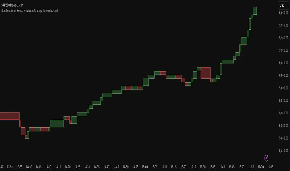
Optimized Heikin Ashi Strategy with Buy/Sell OptionsStrategy Name:
Optimized Heikin Ashi Strategy with Buy/Sell Options
Description:
The Optimized Heikin Ashi Strategy is a trend-following strategy designed to capitalize on market trends by utilizing the smoothness of Heikin Ashi candles. This strategy provides flexible options for trading, allowing users to choose between Buy Only (long-only), Sell Only (short-only), or using both in alternating conditions based on the Heikin Ashi candle signals. The strategy works on any market, but it performs especially well in markets where trends are prevalent, such as cryptocurrency or Forex.
This script offers customizable parameters for the backtest period, Heikin Ashi timeframe, stop loss, and take profit levels, allowing traders to optimize the strategy for their preferred markets or assets.
Key Features:
Trade Type Options:
Buy Only: Enter a long position when a green Heikin Ashi candle appears and exit when a red candle appears.
Sell Only: Enter a short position when a red Heikin Ashi candle appears and exit when a green candle appears.
Stop Loss and Take Profit:
Customizable stop loss and take profit percentages allow for flexible risk management.
The default stop loss is set to 2%, and the default take profit is set to 4%, maintaining a favorable risk/reward ratio.
Heikin Ashi Timeframe:
Traders can select the desired timeframe for Heikin Ashi candle calculation (e.g., 4-hour Heikin Ashi candles for a 1-hour chart).
The strategy smooths out price action and reduces noise, providing clearer signals for entry and exit.
Inputs:
Backtest Start Date / End Date: Specify the period for testing the strategy’s performance.
Heikin Ashi Timeframe: Select the timeframe for Heikin Ashi candle generation. A higher timeframe helps smooth the trend, which is beneficial for trading lower timeframes.
Stop Loss (in %) and Take Profit (in %): Enable or disable stop loss and take profit, and adjust the levels based on market conditions.
Trade Type: Choose between Buy Only or Sell Only based on your market outlook and strategy preference.
Strategy Performance:
In testing with BTC/USD, this strategy performed well in a 4-hour Heikin Ashi timeframe applied on a 1-hour chart over a period from January 1, 2024, to September 12, 2024. The results were as follows:
Initial Capital: 1 USD
Order Size: 100% of equity
Net Profit: +30.74 USD (3,073.52% return)
Percent Profitable: 78.28% of trades were winners.
Profit Factor: 15.825, indicating that the strategy's profitable trades far outweighed its losses.
Max Drawdown: 4.21%, showing low risk exposure relative to the large profit potential.
This strategy is ideal for both beginner and advanced traders who are looking to follow trends and avoid market noise by using Heikin Ashi candles. It is also well-suited for traders who prefer automated risk management through the use of stop loss and take profit levels.
Recommended Use:
Best Markets: This strategy works well on trending markets like cryptocurrency, Forex, or indices.
Timeframes: Works best when applied to lower timeframes (e.g., 1-hour chart) with a higher Heikin Ashi timeframe (e.g., 4-hour candles) to smooth out price action.
Leverage: The strategy performs well with leverage, but users should consider using 2x to 3x leverage to avoid excessive risk and potential liquidation. The strategy's low drawdown allows for moderate leverage use while maintaining risk control.
Customization: Traders can adjust the stop loss and take profit percentages based on their risk appetite and market conditions. A default setting of a 2% stop loss and 4% take profit provides a balanced risk/reward ratio.
Notes:
Risk Management: Traders should enable stop loss and take profit settings to maintain effective risk management and prevent large drawdowns during volatile market conditions.
Optimization: This strategy can be further optimized by adjusting the Heikin Ashi timeframe and risk parameters based on specific market conditions and assets.
Backtesting: The built-in backtesting functionality allows traders to test the strategy across different market conditions and historical data to ensure robustness before applying it to live trading.
How to Apply:
Select your preferred market and chart.
Choose the appropriate Heikin Ashi timeframe based on the chart's timeframe. (e.g., use 4-hour Heikin Ashi candles for 1-hour chart trends).
Adjust stop loss and take profit based on your risk management preference.
Run backtesting to evaluate its performance before applying it in live trading.
This strategy can be further modified and optimized based on personal trading style and market conditions. It’s important to monitor performance regularly and adjust settings as needed to align with market behavior.

Fibonacci-Only StrategyFibonacci-Only Strategy
This script is a custom trading strategy designed for traders who leverage Fibonacci retracement levels to identify potential trade entries and exits. The strategy is versatile, allowing users to trade across multiple timeframes, with built-in options for dynamic stop loss, trailing stops, and take profit levels.
Key Features:
Custom Fibonacci Levels:
This strategy calculates three specific Fibonacci retracement levels: 19%, 82.56%, and the reverse 19% level. These levels are used to identify potential areas of support and resistance where price reversals or breaks might occur.
The Fibonacci levels are calculated based on the highest and lowest prices within a 100-bar period, making them dynamic and responsive to recent market conditions.
Dynamic Entry Conditions:
Touch Entry: The script enters long or short positions when the price touches specific Fibonacci levels and confirms the move with a bullish (for long) or bearish (for short) candle.
Break Entry (Optional): If the "Use Break Strategy" option is enabled, the script can also enter positions when the price breaks through Fibonacci levels, providing more aggressive entry opportunities.
Stop Loss Management:
The script offers flexible stop loss settings. Users can choose between a fixed percentage stop loss or an ATR-based stop loss, which adjusts based on market volatility.
The ATR (Average True Range) stop loss is multiplied by a user-defined factor, allowing for tailored risk management based on market conditions.
Trailing Stop Mechanism:
The script includes an optional trailing stop feature, which adjusts the stop loss level as the market moves in favor of the trade. This helps lock in profits while allowing the trade to run if the trend continues.
The trailing stop is calculated as a percentage of the difference between the entry price and the current market price.
Multiple Take Profit Levels:
The strategy calculates seven take profit levels, each at incremental percentages above (for long trades) or below (for short trades) the entry price. This allows for gradual profit-taking as the market moves in the trade's favor.
Each take profit level can be customized in terms of the percentage of the position to be closed, providing precise control over exit strategies.
Strategy Backtesting and Results:
Realistic Backtesting:
The script has been backtested with realistic account sizes, commission rates, and slippage settings to ensure that the results are applicable to actual trading scenarios.
The backtesting covers various timeframes and markets to ensure the strategy's robustness across different trading environments.
Default Settings:
The script is published with default settings that have been optimized for general use. These settings include a 15-minute timeframe, a 1.0% stop loss, a 2.0 ATR multiplier for stop loss, and a 1.5% trailing stop.
Users can adjust these settings to better fit their specific trading style or the market they are trading.
How It Works:
Long Entry Conditions:
The strategy enters a long position when the price touches the 19% Fibonacci level (from high to low) or the reverse 19% level (from low to high) and confirms the move with a bullish candle.
If the "Use Break Strategy" option is enabled, the script will also enter a long position when the price breaks below the 19% Fibonacci level and then moves back up, confirming the break with a bullish candle.
Short Entry Conditions:
The strategy enters a short position when the price touches the 82.56% Fibonacci level and confirms the move with a bearish candle.
If the "Use Break Strategy" option is enabled, the script will also enter a short position when the price breaks above the 82.56% Fibonacci level and then moves back down, confirming the break with a bearish candle.
Stop Loss and Take Profit Logic:
The stop loss for each trade is calculated based on the selected method (fixed percentage or ATR-based). The strategy then manages the trade by either trailing the stop or taking profit at predefined levels.
The take profit levels are set at increments of 0.5% above or below the entry price, depending on whether the position is long or short. The script gradually exits the trade as these levels are hit, securing profits while minimizing risk.
Usage:
For Fibonacci Traders:
This script is ideal for traders who rely on Fibonacci retracement levels to find potential trade entries and exits. The script automates the process, allowing traders to focus on market analysis and decision-making.
For Trend and Swing Traders:
The strategy's flexibility in handling both touch and break entries makes it suitable for trend-following and swing trading strategies. The multiple take profit levels allow traders to capture profits in trending markets while managing risk.
Important Notes:
Originality: This script uniquely combines Fibonacci retracement levels with dynamic stop loss management and multiple take profit levels. It is not just a combination of existing indicators but a thoughtful integration designed to enhance trading performance.
Disclaimer: Trading involves risk, and it is crucial to test this script in a demo account or through backtesting before applying it to live trading. Users should ensure that the settings align with their individual risk tolerance and trading strategy.

TENKAN SCALPER STRATEGYTENKAN SCALP is a fully automatic trading system.
It is a continuation of our previous ichimoku release. This time however we throw out the rule book and use ICHIMOKU in a very different way.
It applies non traditional money management tactics.
While most trading strategies rely on a stop loss and a take profit target to manage risk. This strategy uses either no stop loss at all or a time based stop loss.
You might ask yourself the question why would you keep a trade open if it goes against you? Here are a phew reasons why the script does what it does.
Forex Markets consolidate most of the time. If you wait long enough your Take Profit will get hit anyways most of the time
You don't have to risk everything per trade. I keep my orders small so to keep some powder to get into some more trades
All the extra trades you take while one trade is in drawdown limit the drawdown as they provide cashflow
On lower timeframes the markets are so chaotic that a stop loss is very likely to get hit by a wick
About backtest below
This backtest uses a spread of 2 pips for entries and a default position size of 100% of equity. This is only possible on exchanges where spread is low and you have 10:1 leverage or more. It does not represent results obtainable without leverage. Do take into account that there are a lot of forex exchanges that provide this leverage, however a 2 pip spread is not always guaranteed and only applies to major pairs.
This backtest does not use the TIME BASED STOPS functionality.
Always start with small position sizing and see how the strategy performs before adding risk.
Explanation of variables:
Chikou(lagging span): pink line, this is price plotted 26 bars ago. People ignore the power of this it is crucial to see how chikou behaves towards past price action as seen in the chart below where we got an entry at red arrow because chikou bounced from past fractal bottom.
Kijun-Sen(base line): Black line or color coded line. This is the equilibrium of last 26 candles. To me this is the most important line in the system as it attracts price.
Kijun = (Highest high of 26 periods + Lowest low of 26 periods) ÷ 2
Tenkan-Sen(conversion line): Blue line. This is the equilibrium of last 9 candles. In a strong uptrend price stays above this line.
Tenkan = (Highest high of 9 periods + Lowest low of 9 periods) ÷ 2
Senkou A (Leading span A)= Pink cloud line, this is the average of the 2 components projected 26 bars in the future.
Senkou A = (Tenkan + Kijun) ÷ 2
Senkou B (Leading span B) = Green cloud line, this is the 52 day equilibrium projected 26 bars in the future.
Senkou B = (Highest high of prior 52 periods + Lowest low of prior 52 periods) ÷ 2
projection: Script uses same function for variable calculation and substracts a number on each next bar as to make a projection of where the variable will be in future bars if price stayed the same. This works as ICHIMOKU calculations use the middle point of a past set of data. The shorter that amount of bars will be in line with the data that it will be restricted to in future if price stayed the same.
Detection of Market Environment
To enter trades the script uses a lot of ICHIMOKU concepts. Contrary to how most people trade ICHIMOKU this script takes an environment that ICHIMOKU identifies as trending upwards and shorts in that environment. The same will be applied to a downtrend where it will open LONGS.
List of CRITERIA for a trend:
Grapling Hook: this is a component based on the chikou span (closing price displaced 26 bars into the past). The script will use an ATR based range to define a possible future projection to the CHIKOU line. For a market to be bullish there should be no price action happening within this area. Market is free to move upwards. Vice versa for bearish .
Kumo Cloud: script will check if price is above the cloud for bullish trend and below cloud for bearish trend .
Chikou above Kijun: script will check if the chikou line is above the KIJUN line of 26 bars ago. This is further confirmation that price is trending high enough compared to it's past data. Vice versa for downtrend.
Kijun projection: script will check if past Kijun is lower than future projected Kijun. This to ensure we get an equilibrium in our favour in the future. Vice versa for downtrend
Tenkan projection: script will check if future Tenkan-sen will be higher than Kijun-sen for an uptrend. Vice versa for downtrend.
Cloud projection: script will check if in 9 bars the Senkou Span A will be higher than Senkou Span B for an uptrend. Vice versa for downtrend.
Example:
This script does not visualise the prediction lines like I show in the example. I show them here to clarify how the script works.
Usage
Backtests are not indicative of future results, although a trader may want to use a strategy script to have a deeper understanding of how their strategy responds to varying market conditions, or as a tool for identifying possible flaws for a strategy that may be indicative of good or bad performance in the future.
Strategy Settings:
Minimum Body Size (atr): this is the minimum ATR a signal bar needs to be for entry. This is useful because our TP is based on previous bar.
Lot size per trade: this setting does not impact backtest. It is used to for the signals to let tradingconnect.com know your position size.
Direction: do you want to trade longs or shorts. I personally use both a long bot and a short bot at the same time.
Positions Allowed: the amount of positions the script will keep open as a maximum. You do not want to open too many positions, this is for risk management.
Close all positions at drawdown: if total open positions loss gets to this % target it will close all positions.
MetaTrader Prefix: when the script sends a signal it will put this text right before the symbol name from syminfo.ticker
MetaTrader Suffix: when the script sends a signal it will put this text right after the symbol name from syminfo.ticker
Charts below are some examples on how the script handles orders on default settings:
without time based SL
with time based SL
how it handles pyramiding
www.tradingview.com
Tradingconnector.com:
For full automation of the forex market the script uses this connector to execute trade on MT4. The alerts the script sends using the alerts() function call are structured in a way tradingconnector will recognise and send directly to MT4. You can find documentation about this tool on their own website.
Personal recommendation is to start with a minimum lot size and track performance, if you are comfortable scale the size up. You can do that by increasing the lot size setting in the script and making a new alert. Make sure to delete the old one.
How to access
You can see the Author's Instructions below to visit our telegram to get more information on how to get access.

The Barking Rat ReversionsMean Reversion with Multi-Layered Precision
The Barking Rat Reversions is a short-term mean reversion strategy tailored for high-volatility markets. It combines several well-established technical tools in a configuration to identify overextended price movements likely to revert toward equilibrium. The goal is to isolate high-quality, short-term reversal opportunities while filtering out low-conviction setups.
At its core, our strategy triggers off Fair Value Gaps (FVGs) that occur a considerable distance away from a dynamically defined equilibrium band. It then validates these gaps by checking proximity to recent support and resistance drawn from swing extremes.
Additional confirmation comes from momentum filters and wick-rejection patterns, ensuring each entry aligns with both price structure and stretched momentum. Exits use volatility-adjusted profit targets. Keeping the approach disciplined and adaptive.
🧠Core Logic: Selectivity & Structure
This strategy is intentionally very selective. We have designed it to filter out roughly 95% of all market noise, highlighting only setups that pass multiple validation layers outlined below.
Fair Value Gaps (FVGs) as the Primary Trigger
FVGs identify imbalance zones where price historically retraces. These inefficient zones often become magnets for reversion as the market seeks to rebalance.
Dynamic Equilibrium Band + S/R
Defines a fair value zone with a long-term moving average and combines it with shorter-term swing pivots to establish support/resistance. Only FVGs that occur outside the band and near recent pivots are considered, ensuring reversals are sufficiently distanced and not taken too close to the mean.
Proximity to Support/Resistance
Setup validity depends on location. The strategy filters for FVGs near well-defined structural levels — areas where price has previously turned (i.e., recent swing highs or lows). This increases the likelihood that reversals are occurring at legitimate zones of confluence.
Wick-Rejection Confirmation
Confirms potential exhaustion through characteristic candle wick patterns beyond the equilibrium region. This acts as another filter to improve signal accuracy.
Sequential Filtered Signals
Custom logic ensures that a new signal in any direction must improve upon the previous one, preventing repetitive or suboptimal entries.
Multi-Step Confirmation
All validation layers must coincide on the same bar before a signal triggers, dramatically reducing false positives.
📈Chart Visuals: Designed for Clarity
To ensure transparency and easy interpretation, the script overlays intuitive visuals:
Green “▲” below a candle: Indicates a potential long entry
Red “▼” above a candle: Indicates a potential short entry
Green “✔️”: Marks exit from a trade when ATR target is met
Background shading (green/red): Indicates trade direction while active
Support/Resistance lines: Auto-plotted from recent swing levels
🔔Alerts: Stay Notified Without Watching
The strategy supports real-time alerts on candle close, ensuring that signals are only triggered once fully confirmed.
You must manually set up alerts within your TradingView account. Once configured, you’ll be able to set up one alert per instrument. This one alert covers all relevant signals and exits — ideal for hands-free monitoring.
⚙️Strategy report properties
Position size: 25% equity per trade
Initial capital: 10,000.00 USDT
Pyramiding: 10 entries per direction
Slippage: 2 ticks
Commission: 0.055% per side
Backtest timeframe: 1-minute
Backtest instrument: HYPEUSDT
Backtesting range: Jul 21, 2025 — Aug 7, 2025
Note on Sample Size:
You’ll notice the report displays fewer than the ideal 100 trades in the strategy report above. This is intentional. The goal of the script is to isolate high-quality, short-term reversal opportunities while filtering out low-conviction setups. This means that the Barking Rat Reversions strategy is ultra-selective, filtering out over 95% of market noise by enforcing multiple validation layers. The brief timeframe shown in the strategy report here illustrates its filtering logic over a short window — not its full capabilities. As a result, even on lower timeframes like the 1-minute chart, signals are deliberately sparse — each one must pass all criteria before triggering.
We conducted a broader backtest covering the period from December 5, 2024 to July 31, 2025, during which the strategy identified 968 high-probability setups on the same instrument and timeframe as the strategy report.
For a larger dataset:
Once the strategy is applied to your chart, users are encouraged to expand the lookback range or apply the strategy to other volatile pairs to view a full sample.
💡Why 25% Equity Per Trade?
While it's always best to size positions based on personal risk tolerance, we defaulted to 25% equity per trade in the backtesting data — and here’s why:
Backtests using this sizing show manageable drawdowns even under volatile periods
The strategy generates a sizeable number of trades, reducing reliance on a single outcome
Combined with conservative filters, the 25% setting offers a balance between aggression and control
Users are strongly encouraged to customize this to suit their risk profile.
🔍What Makes This Strategy Unique?
Multi-factor confirmation using FVGs, EMA deviation, RSI, wick rejection, and S/R
Clean, Intuitive Chart Experience
Real-time alerts triggered only on confirmation
Variables monitor prior reversal points, guaranteeing each new signal offers an improved entry
Tracks active positions and resets filters upon exit.

Bober XM v2.0# ₿ober XM v2.0 Trading Bot Documentation
**Developer's Note**: While our previous Bot 1.3.1 was removed due to guideline violations, this setback only fueled our determination to create something even better. Rising from this challenge, Bober XM 2.0 emerges not just as an update, but as a complete reimagining with multi-timeframe analysis, enhanced filters, and superior adaptability. This adversity pushed us to innovate further and deliver a strategy that's smarter, more agile, and more powerful than ever before. Challenges create opportunity - welcome to Cryptobeat's finest work yet.
## !!!!You need to tune it for your own pair and timeframe and retune it periodicaly!!!!!
## Overview
The ₿ober XM v2.0 is an advanced dual-channel trading bot with multi-timeframe analysis capabilities. It integrates multiple technical indicators, customizable risk management, and advanced order execution via webhook for automated trading. The bot's distinctive feature is its separate channel systems for long and short positions, allowing for asymmetric trade strategies that adapt to different market conditions across multiple timeframes.
### Key Features
- **Multi-Timeframe Analysis**: Analyze price data across multiple timeframes simultaneously
- **Dual Channel System**: Separate parameter sets for long and short positions
- **Advanced Entry Filters**: RSI, Volatility, Volume, Bollinger Bands, and KEMAD filters
- **Machine Learning Moving Average**: Adaptive prediction-based channels
- **Multiple Entry Strategies**: Breakout, Pullback, and Mean Reversion modes
- **Risk Management**: Customizable stop-loss, take-profit, and trailing stop settings
- **Webhook Integration**: Compatible with external trading bots and platforms
### Strategy Components
| Component | Description |
|---------|-------------|
| **Dual Channel Trading** | Uses either Keltner Channels or Machine Learning Moving Average (MLMA) with separate settings for long and short positions |
| **MLMA Implementation** | Machine learning algorithm that predicts future price movements and creates adaptive bands |
| **Pivot Point SuperTrend** | Trend identification and confirmation system based on pivot points |
| **Three Entry Strategies** | Choose between Breakout, Pullback, or Mean Reversion approaches |
| **Advanced Filter System** | Multiple customizable filters with multi-timeframe support to avoid false signals |
| **Custom Exit Logic** | Exits based on OBV crossover of its moving average combined with pivot trend changes |
### Note for Novice Users
This is a fully featured real trading bot and can be tweaked for any ticker — SOL is just an example. It follows this structure:
1. **Indicator** – gives the initial signal
2. **Entry strategy** – decides when to open a trade
3. **Exit strategy** – defines when to close it
4. **Trend confirmation** – ensures the trade follows the market direction
5. **Filters** – cuts out noise and avoids weak setups
6. **Risk management** – controls losses and protects your capital
To tune it for a different pair, you'll need to start from scratch:
1. Select the timeframe (candle size)
2. Turn off all filters and trend entry/exit confirmations
3. Choose a channel type, channel source and entry strategy
4. Adjust risk parameters
5. Tune long and short settings for the channel
6. Fine-tune the Pivot Point Supertrend and Main Exit condition OBV
This will generate a lot of signals and activity on the chart. Your next task is to find the right combination of filters and settings to reduce noise and tune it for profitability.
### Default Strategy values
Default values are tuned for: Symbol BITGET:SOLUSDT.P 5min candle
Filters are off by default: Try to play with it to understand how it works
## Configuration Guide
### General Settings
| Setting | Description | Default Value |
|---------|-------------|---------------|
| **Long Positions** | Enable or disable long trades | Enabled |
| **Short Positions** | Enable or disable short trades | Enabled |
| **Risk/Reward Area** | Visual display of stop-loss and take-profit zones | Enabled |
| **Long Entry Source** | Price data used for long entry signals | hl2 (High+Low/2) |
| **Short Entry Source** | Price data used for short entry signals | hl2 (High+Low/2) |
The bot allows you to trade long positions, short positions, or both simultaneously. Each direction has its own set of parameters, allowing for fine-tuned strategies that recognize the asymmetric nature of market movements.
### Multi-Timeframe Settings
1. **Enable Multi-Timeframe Analysis**: Toggle 'Enable Multi-Timeframe Analysis' in the Multi-Timeframe Settings section
2. **Configure Timeframes**: Set appropriate higher timeframes based on your trading style:
- Timeframe 1: Default is now 15 minutes (intraday confirmation)
- Timeframe 2: Default is 4 hours (trend direction)
3. **Select Sources per Indicator**: For each indicator (RSI, KEMAD, Volume, etc.), choose:
- The desired timeframe (current, mtf1, or mtf2)
- The appropriate price type (open, high, low, close, hl2, hlc3, ohlc4)
### Entry Strategies
- **Breakout**: Enter when price breaks above/below the channel
- **Pullback**: Enter when price pulls back to the channel
- **Mean Reversion**: Enter when price is extended from the channel
You can enable different strategies for long and short positions.
### Core Components
### Risk Management
- **Position Size**: Control risk with percentage-based position sizing
- **Stop Loss Options**:
- Fixed: Set a specific price or percentage from entry
- ATR-based: Dynamic stop-loss based on market volatility
- Swing: Uses recent swing high/low points
- **Take Profit**: Multiple targets with percentage allocation
- **Trailing Stop**: Dynamic stop that follows price movement
## Advanced Usage Strategies
### Moving Average Type Selection Guide
- **SMA**: More stable in choppy markets, good for higher timeframes
- **EMA/WMA**: More responsive to recent price changes, better for entry signals
- **VWMA**: Adds volume weighting for stronger trends, use with Volume filter
- **HMA**: Balance between responsiveness and noise reduction, good for volatile markets
### Multi-Timeframe Strategy Approaches
- **Trend Confirmation**: Use higher timeframe RSI (mtf2) for overall trend, current timeframe for entries
- **Entry Precision**: Use KEMAD on current timeframe with volume filter on mtf1
- **False Signal Reduction**: Apply RSI filter on mtf1 with strict KEMAD settings
### Market Condition Optimization
| Market Condition | Recommended Settings |
|------------------|----------------------|
| **Trending** | Use Breakout strategy with KEMAD filter on higher timeframe |
| **Ranging** | Use Mean Reversion with strict RSI filter (mtf1) |
| **Volatile** | Increase ATR multipliers, use HMA for moving averages |
| **Low Volatility** | Decrease noise parameters, use pullback strategy |
## Webhook Integration
The strategy features a professional webhook system that allows direct connectivity to your exchange or trading platform of choice through third-party services like 3commas, Alertatron, or Autoview.
The webhook payload includes all necessary parameters for automated execution:
- Entry price and direction
- Stop loss and take profit levels
- Position size
- Custom identifier for webhook routing
## Performance Optimization Tips
1. **Start with Defaults**: Begin with the default settings for your timeframe before customizing
2. **Adjust One Component at a Time**: Make incremental changes and test the impact
3. **Match MA Types to Market Conditions**: Use appropriate moving average types based on the Market Condition Optimization table
4. **Timeframe Synergy**: Create logical relationships between timeframes (e.g., 5min chart with 15min and 4h higher timeframes)
5. **Periodic Retuning**: Markets evolve - regularly review and adjust parameters
## Common Setups
### Crypto Trend-Following
- MLMA with EMA or HMA
- Higher RSI thresholds (75/25)
- KEMAD filter on mtf1
- Breakout entry strategy
### Stock Swing Trading
- MLMA with SMA for stability
- Volume filter with higher threshold
- KEMAD with increased filter order
- Pullback entry strategy
### Forex Scalping
- MLMA with WMA and lower noise parameter
- RSI filter on current timeframe
- Use highest timeframe for trend direction only
- Mean Reversion strategy
## Webhook Configuration
- **Benefits**:
- Automated trade execution without manual intervention
- Immediate response to market conditions
- Consistent execution of your strategy
- **Implementation Notes**:
- Requires proper webhook configuration on your exchange or platform
- Test thoroughly with small position sizes before full deployment
- Consider latency between signal generation and execution
### Backtesting Period
Define a specific historical period to evaluate the bot's performance:
| Setting | Description | Default Value |
|---------|-------------|---------------|
| **Start Date** | Beginning of backtest period | January 1, 2025 |
| **End Date** | End of backtest period | December 31, 2026 |
- **Best Practice**: Test across different market conditions (bull markets, bear markets, sideways markets)
- **Limitation**: Past performance doesn't guarantee future results
## Entry and Exit Strategies
### Dual-Channel System
A key innovation of the Bober XM is its dual-channel approach:
- **Independent Parameters**: Each trade direction has its own channel settings
- **Asymmetric Trading**: Recognizes that markets often behave differently in uptrends versus downtrends
- **Optimized Performance**: Fine-tune settings for both bullish and bearish conditions
This approach allows the bot to adapt to the natural asymmetry of markets, where uptrends often develop gradually while downtrends can be sharp and sudden.
### Channel Types
#### 1. Keltner Channels
Traditional volatility-based channels using EMA and ATR:
| Setting | Long Default | Short Default |
|---------|--------------|---------------|
| **EMA Length** | 37 | 20 |
| **ATR Length** | 13 | 17 |
| **Multiplier** | 1.4 | 1.9 |
| **Source** | low | high |
- **Strengths**:
- Reliable in trending markets
- Less prone to whipsaws than Bollinger Bands
- Clear visual representation of volatility
- **Weaknesses**:
- Can lag during rapid market changes
- Less effective in choppy, non-trending markets
#### 2. Machine Learning Moving Average (MLMA)
Advanced predictive model using kernel regression (RBF kernel):
| Setting | Description | Options |
|---------|-------------|--------|
| **Source MA** | Price data used for MA calculations | Any price source (low/high/close/etc.) |
| **Moving Average Type** | Type of MA algorithm for calculations | SMA, EMA, WMA, VWMA, RMA, HMA |
| **Trend Source** | Price data used for trend determination | Any price source (close default) |
| **Window Size** | Historical window for MLMA calculations | 5+ (default: 16) |
| **Forecast Length** | Number of bars to forecast ahead | 1+ (default: 3) |
| **Noise Parameter** | Controls smoothness of prediction | 0.01+ (default: ~0.43) |
| **Band Multiplier** | Multiplier for channel width | 0.1+ (default: 0.5-0.6) |
- **Strengths**:
- Predictive rather than reactive
- Adapts quickly to changing market conditions
- Better at identifying trend reversals early
- **Weaknesses**:
- More computationally intensive
- Requires careful parameter tuning
- Can be sensitive to input data quality
### Entry Strategies
| Strategy | Description | Ideal Market Conditions |
|----------|-------------|-------------------------|
| **Breakout** | Enters when price breaks through channel bands, indicating strong momentum | High volatility, emerging trends |
| **Pullback** | Enters when price retraces to the middle band after testing extremes | Established trends with regular pullbacks |
| **Mean Reversion** | Enters at channel extremes, betting on a return to the mean | Range-bound or oscillating markets |
#### Breakout Strategy (Default)
- **Implementation**: Enters long when price crosses above the upper band, short when price crosses below the lower band
- **Strengths**: Captures strong momentum moves, performs well in trending markets
- **Weaknesses**: Can lead to late entries, higher risk of false breakouts
- **Optimization Tips**:
- Increase channel multiplier for fewer but more reliable signals
- Combine with volume confirmation for better accuracy
#### Pullback Strategy
- **Implementation**: Enters long when price pulls back to middle band during uptrend, short during downtrend pullbacks
- **Strengths**: Better entry prices, lower risk, higher probability setups
- **Weaknesses**: Misses some strong moves, requires clear trend identification
- **Optimization Tips**:
- Use with trend filters to confirm overall direction
- Adjust middle band calculation for market volatility
#### Mean Reversion Strategy
- **Implementation**: Enters long at lower band, short at upper band, expecting price to revert to the mean
- **Strengths**: Excellent entry prices, works well in ranging markets
- **Weaknesses**: Dangerous in strong trends, can lead to fighting the trend
- **Optimization Tips**:
- Implement strong trend filters to avoid counter-trend trades
- Use smaller position sizes due to higher risk nature
### Confirmation Indicators
#### Pivot Point SuperTrend
Combines pivot points with ATR-based SuperTrend for trend confirmation:
| Setting | Default Value |
|---------|---------------|
| **Pivot Period** | 25 |
| **ATR Factor** | 2.2 |
| **ATR Period** | 41 |
- **Function**: Identifies significant market turning points and confirms trend direction
- **Implementation**: Requires price to respect the SuperTrend line for trade confirmation
#### Weighted Moving Average (WMA)
Provides additional confirmation layer for entries:
| Setting | Default Value |
|---------|---------------|
| **Period** | 15 |
| **Source** | ohlc4 (average of Open, High, Low, Close) |
- **Function**: Confirms trend direction and filters out low-quality signals
- **Implementation**: Price must be above WMA for longs, below for shorts
### Exit Strategies
#### On-Balance Volume (OBV) Based Exits
Uses volume flow to identify potential reversals:
| Setting | Default Value |
|---------|---------------|
| **Source** | ohlc4 |
| **MA Type** | HMA (Options: SMA, EMA, WMA, RMA, VWMA, HMA) |
| **Period** | 22 |
- **Function**: Identifies divergences between price and volume to exit before reversals
- **Implementation**: Exits when OBV crosses its moving average in the opposite direction
- **Customizable MA Type**: Different MA types provide varying sensitivity to OBV changes:
- **SMA**: Traditional simple average, equal weight to all periods
- **EMA**: More weight to recent data, responds faster to price changes
- **WMA**: Weighted by recency, smoother than EMA
- **RMA**: Similar to EMA but smoother, reduces noise
- **VWMA**: Factors in volume, helpful for OBV confirmation
- **HMA**: Reduces lag while maintaining smoothness (default)
#### ADX Exit Confirmation
Uses Average Directional Index to confirm trend exhaustion:
| Setting | Default Value |
|---------|---------------|
| **ADX Threshold** | 35 |
| **ADX Smoothing** | 60 |
| **DI Length** | 60 |
- **Function**: Confirms trend weakness before exiting positions
- **Implementation**: Requires ADX to drop below threshold or DI lines to cross
## Filter System
### RSI Filter
- **Function**: Controls entries based on momentum conditions
- **Parameters**:
- Period: 15 (default)
- Overbought level: 71
- Oversold level: 23
- Multi-timeframe support: Current, MTF1 (15min), or MTF2 (4h)
- Customizable price source (open, high, low, close, hl2, hlc3, ohlc4)
- **Implementation**: Blocks long entries when RSI > overbought, short entries when RSI < oversold
### Volatility Filter
- **Function**: Prevents trading during excessive market volatility
- **Parameters**:
- Measure: ATR (Average True Range)
- Period: Customizable (default varies by timeframe)
- Threshold: Adjustable multiplier
- Multi-timeframe support
- Customizable price source
- **Implementation**: Blocks trades when current volatility exceeds threshold × average volatility
### Volume Filter
- **Function**: Ensures adequate market liquidity for trades
- **Parameters**:
- Threshold: 0.4× average (default)
- Measurement period: 5 (default)
- Moving average type: Customizable (HMA default)
- Multi-timeframe support
- Customizable price source
- **Implementation**: Requires current volume to exceed threshold × average volume
### Bollinger Bands Filter
- **Function**: Controls entries based on price relative to statistical boundaries
- **Parameters**:
- Period: Customizable
- Standard deviation multiplier: Adjustable
- Moving average type: Customizable
- Multi-timeframe support
- Customizable price source
- **Implementation**: Can require price to be within bands or breaking out of bands depending on strategy
### KEMAD Filter (Kalman EMA Distance)
- **Function**: Advanced trend confirmation using Kalman filter algorithm
- **Parameters**:
- Process Noise: 0.35 (controls smoothness)
- Measurement Noise: 24 (controls reactivity)
- Filter Order: 6 (higher = more smoothing)
- ATR Length: 8 (for bandwidth calculation)
- Upper Multiplier: 2.0 (for long signals)
- Lower Multiplier: 2.7 (for short signals)
- Multi-timeframe support
- Customizable visual indicators
- **Implementation**: Generates signals based on price position relative to Kalman-filtered EMA bands
## Risk Management System
### Position Sizing
Automatically calculates position size based on account equity and risk parameters:
| Setting | Default Value |
|---------|---------------|
| **Risk % of Equity** | 50% |
- **Implementation**:
- Position size = (Account equity × Risk %) ÷ (Entry price × Stop loss distance)
- Adjusts automatically based on volatility and stop placement
- **Best Practices**:
- Start with lower risk percentages (1-2%) until strategy is proven
- Consider reducing risk during high volatility periods
### Stop-Loss Methods
Multiple stop-loss calculation methods with separate configurations for long and short positions:
| Method | Description | Configuration |
|--------|-------------|---------------|
| **ATR-Based** | Dynamic stops based on volatility | ATR Period: 14, Multiplier: 2.0 |
| **Percentage** | Fixed percentage from entry | Long: 1.5%, Short: 1.5% |
| **PIP-Based** | Fixed currency unit distance | 10.0 pips |
- **Implementation Notes**:
- ATR-based stops adapt to changing market volatility
- Percentage stops maintain consistent risk exposure
- PIP-based stops provide precise control in stable markets
### Trailing Stops
Locks in profits by adjusting stop-loss levels as price moves favorably:
| Setting | Default Value |
|---------|---------------|
| **Stop-Loss %** | 1.5% |
| **Activation Threshold** | 2.1% |
| **Trailing Distance** | 1.4% |
- **Implementation**:
- Initial stop remains fixed until profit reaches activation threshold
- Once activated, stop follows price at specified distance
- Locks in profit while allowing room for normal price fluctuations
### Risk-Reward Parameters
Defines the relationship between risk and potential reward:
| Setting | Default Value |
|---------|---------------|
| **Risk-Reward Ratio** | 1.4 |
| **Take Profit %** | 2.4% |
| **Stop-Loss %** | 1.5% |
- **Implementation**:
- Take profit distance = Stop loss distance × Risk-reward ratio
- Higher ratios require fewer winning trades for profitability
- Lower ratios increase win rate but reduce average profit
### Filter Combinations
The strategy allows for simultaneous application of multiple filters:
- **Recommended Combinations**:
- Trending markets: RSI + KEMAD filters
- Ranging markets: Bollinger Bands + Volatility filters
- All markets: Volume filter as minimum requirement
- **Performance Impact**:
- Each additional filter reduces the number of trades
- Quality of remaining trades typically improves
- Optimal combination depends on market conditions and timeframe
### Multi-Timeframe Filter Applications
| Filter Type | Current Timeframe | MTF1 (15min) | MTF2 (4h) |
|-------------|-------------------|-------------|------------|
| RSI | Quick entries/exits | Intraday trend | Overall trend |
| Volume | Immediate liquidity | Sustained support | Market participation |
| Volatility | Entry timing | Short-term risk | Regime changes |
| KEMAD | Precise signals | Trend confirmation | Major reversals |
## Visual Indicators and Chart Analysis
The bot provides comprehensive visual feedback on the chart:
- **Channel Bands**: Keltner or MLMA bands showing potential support/resistance
- **Pivot SuperTrend**: Colored line showing trend direction and potential reversal points
- **Entry/Exit Markers**: Annotations showing actual trade entries and exits
- **Risk/Reward Zones**: Visual representation of stop-loss and take-profit levels
These visual elements allow for:
- Real-time strategy assessment
- Post-trade analysis and optimization
- Educational understanding of the strategy logic
## Implementation Guide
### TradingView Setup
1. Load the script in TradingView Pine Editor
2. Apply to your preferred chart and timeframe
3. Adjust parameters based on your trading preferences
4. Enable alerts for webhook integration
### Webhook Integration
1. Configure webhook URL in TradingView alerts
2. Set up receiving endpoint on your trading platform
3. Define message format matching the bot's output
4. Test with small position sizes before full deployment
### Optimization Process
1. Backtest across different market conditions
2. Identify parameter sensitivity through multiple tests
3. Focus on risk management parameters first
4. Fine-tune entry/exit conditions based on performance metrics
5. Validate with out-of-sample testing
## Performance Considerations
### Strengths
- Adaptability to different market conditions through dual channels
- Multiple layers of confirmation reducing false signals
- Comprehensive risk management protecting capital
- Machine learning integration for predictive edge
### Limitations
- Complex parameter set requiring careful optimization
- Potential over-optimization risk with so many variables
- Computational intensity of MLMA calculations
- Dependency on proper webhook configuration for execution
### Best Practices
- Start with conservative risk settings (1-2% of equity)
- Test thoroughly in demo environment before live trading
- Monitor performance regularly and adjust parameters
- Consider market regime changes when evaluating results
## Conclusion
The ₿ober XM v2.0 represents a significant evolution in trading strategy design, combining traditional technical analysis with machine learning elements and multi-timeframe analysis. The core strength of this system lies in its adaptability and recognition of market asymmetry.
### Market Asymmetry and Adaptive Approach
The strategy acknowledges a fundamental truth about markets: bullish and bearish phases behave differently and should be treated as distinct environments. The dual-channel system with separate parameters for long and short positions directly addresses this asymmetry, allowing for optimized performance regardless of market direction.
### Targeted Backtesting Philosophy
It's counterproductive to run backtests over excessively long periods. Markets evolve continuously, and strategies that worked in previous market regimes may be ineffective in current conditions. Instead:
- Test specific market phases separately (bull markets, bear markets, range-bound periods)
- Regularly re-optimize parameters as market conditions change
- Focus on recent performance with higher weight than historical results
- Test across multiple timeframes to ensure robustness
### Multi-Timeframe Analysis as a Game-Changer
The integration of multi-timeframe analysis fundamentally transforms the strategy's effectiveness:
- **Increased Safety**: Higher timeframe confirmations reduce false signals and improve trade quality
- **Context Awareness**: Decisions made with awareness of larger trends reduce adverse entries
- **Adaptable Precision**: Apply strict filters on lower timeframes while maintaining awareness of broader conditions
- **Reduced Noise**: Higher timeframe data naturally filters market noise that can trigger poor entries
The ₿ober XM v2.0 provides traders with a framework that acknowledges market complexity while offering practical tools to navigate it. With proper setup, realistic expectations, and attention to changing market conditions, it delivers a sophisticated approach to systematic trading that can be continuously refined and optimized.
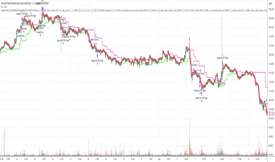
Dskyz (DAFE) Quantum Sentiment Flux - Beginners Dskyz (DAFE) Quantum Sentiment Flux - Beginners:
Welcome to the Dskyz (DAFE) Quantum Sentiment Flux - Beginners , a strategy and concept that’s your ultimate wingman for trading futures like MNQ, NQ, MES, and ES. This gem combines lightning-fast momentum signals, market sentiment smarts, and bulletproof risk management into a system so intuitive, even newbies can trade like pros. With clean DAFE visuals, preset modes for every vibe, and a revamped dashboard that’s basically a market GPS, this strategy makes futures trading feel like a high-octane sci-fi mission.
Built on the Dskyz (DAFE) legacy of Aurora Divergence, the Quantum Sentiment Flux is designed to empower beginners while giving seasoned traders a lean, sentiment-driven edge. It uses fast/slow EMA crossovers for entries, filters trades with VIX, SPX trends, and sector breadth, and keeps your account safe with adaptive stops and cooldowns. Tuned for more action with faster signals and a slick bottom-left dashboard, this updated version is ready to light up your charts and outsmart institutional traps. Let’s dive into why this strat’s a must-have and break down its brilliance.
Why Traders Need This Strategy
Futures markets are a wild ride—fast moves, volatility spikes (like the April 28, 2025 NQ 1k-point drop), and institutional games that can wreck unprepared traders. Beginners often get lost in complex systems or burned by impulsive trades. The Quantum Sentiment Flux is the antidote, offering:
Dead-Simple Setup: Preset modes (Aggressive, Balanced, Conservative) auto-tune signals, risk, and sizing, so you can trade without a quant degree.
Sentiment Superpower: VIX filter, SPX trend, and sector breadth visuals keep you aligned with market health, dodging chop and riding trends.
Ironclad Safety: Tighter ATR-based stops, 2:1 take-profits, and preset cooldowns protect your capital, even in chaotic sessions.
Next-Level Visuals: Green/red entry triangles, vibrant EMAs, a sector breadth background, and a beefed-up dashboard make signals and context pop.
DAFE Swagger: The clean aesthetics, sleek dashboard—ties it to Dskyz’s elite brand, making your charts a work of art.
Traders need this because it’s a plug-and-play system that blends beginner-friendly simplicity with pro-level market awareness. Whether you’re just starting or scalping 5min MNQ, this strat’s your key to trading with confidence and style.
Strategy Components
1. Core Signal Logic (High-Speed Momentum)
The strategy’s engine is a momentum-based system using fast and slow Exponential Moving Averages (EMAs), now tuned for faster, more frequent trades.
How It Works:
Fast/Slow EMAs: Fast EMA (Aggressive: 5, Balanced: 7, Conservative: 9 bars) and slow EMA (12/14/18 bars) track short-term vs. longer-term momentum.
Crossover Signals:
Buy: Fast EMA crosses above slow EMA, and trend_dir = 1 (fast EMA > slow EMA + ATR * strength threshold).
Sell: Fast EMA crosses below slow EMA, and trend_dir = -1 (fast EMA < slow EMA - ATR * strength threshold).
Strength Filter: ma_strength = fast EMA - slow EMA must exceed an ATR-scaled threshold (Aggressive: 0.15, Balanced: 0.18, Conservative: 0.25) for robust signals.
Trend Direction: trend_dir confirms momentum, filtering out weak crossovers in choppy markets.
Evolution:
Faster EMAs (down from 7–10/21–50) catch short-term trends, perfect for active futures markets.
Lower strength thresholds (0.15–0.25 vs. 0.3–0.5) make signals more sensitive, boosting trade frequency without sacrificing quality.
Preset tuning ensures beginners get optimized settings, while pros can tweak via mode selection.
2. Market Sentiment Filters
The strategy leans hard into market sentiment with a VIX filter, SPX trend analysis, and sector breadth visuals, keeping trades aligned with the big picture.
VIX Filter:
Logic: Blocks long entries if VIX > threshold (default: 20, can_long = vix_close < vix_limit). Shorts are always allowed (can_short = true).
Impact: Prevents longs during high-fear markets (e.g., VIX spikes in crashes), while allowing shorts to capitalize on downturns.
SPX Trend Filter:
Logic: Compares S&P 500 (SPX) close to its SMA (Aggressive: 5, Balanced: 8, Conservative: 12 bars). spx_trend = 1 (UP) if close > SMA, -1 (DOWN) if < SMA, 0 (FLAT) if neutral.
Impact: Provides dashboard context, encouraging trades that align with market direction (e.g., longs in UP trend).
Sector Breadth (Visual):
Logic: Tracks 10 sector ETFs (XLK, XLF, XLE, etc.) vs. their SMAs (same lengths as SPX). Each sector scores +1 (bullish), -1 (bearish), or 0 (neutral), summed as breadth (-10 to +10).
Display: Green background if breadth > 4, red if breadth < -4, else neutral. Dashboard shows sector trends (↑/↓/-).
Impact: Faster SMA lengths make breadth more responsive, reflecting sector rotations (e.g., tech surging, energy lagging).
Why It’s Brilliant:
- VIX filter adds pro-level volatility awareness, saving beginners from panic-driven losses.
- SPX and sector breadth give a 360° view of market health, boosting signal confidence (e.g., green BG + buy signal = high-probability trade).
- Shorter SMAs make sentiment visuals react faster, perfect for 5min charts.
3. Risk Management
The risk controls are a fortress, now tighter and more dynamic to support frequent trading while keeping accounts safe.
Preset-Based Risk:
Aggressive: Fast EMAs (5/12), tight stops (1.1x ATR), 1-bar cooldown. High trade frequency, higher risk.
Balanced: EMAs (7/14), 1.2x ATR stops, 1-bar cooldown. Versatile for most traders.
Conservative: EMAs (9/18), 1.3x ATR stops, 2-bar cooldown. Safer, fewer trades.
Impact: Auto-scales risk to match style, making it foolproof for beginners.
Adaptive Stops and Take-Profits:
Logic: Stops = entry ± ATR * atr_mult (1.1–1.3x, down from 1.2–2.0x). Take-profits = entry ± ATR * take_mult (2x stop distance, 2:1 reward/risk). Longs: stop below entry, TP above; shorts: vice versa.
Impact: Tighter stops increase trade turnover while maintaining solid risk/reward, adapting to volatility.
Trade Cooldown:
Logic: Preset-driven (Aggressive/Balanced: 1 bar, Conservative: 2 bars vs. old user-input 2). Ensures bar_index - last_trade_bar >= cooldown.
Impact: Faster cooldowns (especially Aggressive/Balanced) allow more trades, balanced by VIX and strength filters.
Contract Sizing:
Logic: User sets contracts (default: 1, max: 10), no preset cap (unlike old 7/5/3 suggestion).
Impact: Flexible but risks over-leverage; beginners should stick to low contracts.
Built To Be Reliable and Consistent:
- Tighter stops and faster cooldowns make it a high-octane system without blowing up accounts.
- Preset-driven risk removes guesswork, letting newbies trade confidently.
- 2:1 TPs ensure profitable trades outweigh losses, even in volatile sessions like April 27, 2025 ES slippage.
4. Trade Entry and Exit Logic
The entry/exit rules are simple yet razor-sharp, now with VIX filtering and faster signals:
Entry Conditions:
Long Entry: buy_signal (fast EMA crosses above slow EMA, trend_dir = 1), no position (strategy.position_size = 0), cooldown passed (can_trade), and VIX < 20 (can_long). Enters with user-defined contracts.
Short Entry: sell_signal (fast EMA crosses below slow EMA, trend_dir = -1), no position, cooldown passed, can_short (always true).
Logic: Tracks last_entry_bar for visuals, last_trade_bar for cooldowns.
Exit Conditions:
Stop-Loss/Take-Profit: ATR-based stops (1.1–1.3x) and TPs (2x stop distance). Longs exit if price hits stop (below) or TP (above); shorts vice versa.
No Other Exits: Keeps it straightforward, relying on stops/TPs.
5. DAFE Visuals
The visuals are pure DAFE magic, blending clean function with informative metrics utilized by professionals, now enhanced by faster signals and a responsive breadth background:
EMA Plots:
Display: Fast EMA (blue, 2px), slow EMA (orange, 2px), using faster lengths (5–9/12–18).
Purpose: Highlights momentum shifts, with crossovers signaling entries.
Sector Breadth Background:
Display: Green (90% transparent) if breadth > 4, red (90%) if breadth < -4, else neutral.
Purpose: Faster breadth_sma_len (5–12 vs. 10–50) reflects sector shifts in real-time, reinforcing signal strength.
- Visuals are intuitive, turning complex signals into clear buy/sell cues.
- Faster breadth background reacts to market rotations (e.g., tech vs. energy), giving a pro-level edge.
6. Sector Breadth Dashboard
The new bottom-left dashboard is a game-changer, a 3x16 table (black/gray theme) that’s your market command center:
Metrics:
VIX: Current VIX (red if > 20, gray if not).
SPX: Trend as “UP” (green), “DOWN” (red), or “FLAT” (gray).
Trade Longs: “OK” (green) if VIX < 20, “BLOCK” (red) if not.
Sector Breadth: 10 sectors (Tech, Financial, etc.) with trend arrows (↑ green, ↓ red, - gray).
Placeholder Row: Empty for future metrics (e.g., ATR, breadth score).
Purpose: Consolidates regime, volatility, market trend, and sector data, making decisions a breeze.
- VIX and SPX metrics add context, helping beginners avoid bad trades (e.g., no longs if “BLOCK”).
Sector arrows show market health at a glance, like a cheat code for sentiment.
Key Features
Beginner-Ready: Preset modes and clear visuals make futures trading a breeze.
Sentiment-Driven: VIX filter, SPX trend, and sector breadth keep you in sync with the market.
High-Frequency: Faster EMAs, tighter stops, and short cooldowns boost trade volume.
Safe and Smart: Adaptive stops/TPs and cooldowns protect capital while maximizing wins.
Visual Mastery: DAFE’s clean flair, EMAs, dashboard—makes trading fun and clear.
Backtestable: Lean code and fixed qty ensure accurate historical testing.
How to Use
Add to Chart: Load on a 5min MNQ/ES chart in TradingView.
Pick Preset: Aggressive (scalping), Balanced (versatile), or Conservative (safe). Balanced is default.
Set Contracts: Default 1, max 10. Stick low for safety.
Check Dashboard: Bottom-left shows preset, VIX, SPX, and sectors. “OK” + green breadth = strong buy.
Backtest: Run in strategy tester to compare modes.
Live Trade: Connect to Tradovate or similar. Watch for slippage (e.g., April 27, 2025 ES issues).
Replay Test: Try April 28, 2025 NQ drop to see VIX filter and stops in action.
Why It’s Brilliant
The Dskyz (DAFE) Quantum Sentiment Flux - Beginners is a masterpiece of simplicity and power. It takes pro-level tools—momentum, VIX, sector breadth—and wraps them in a system anyone can run. Faster signals and tighter stops make it a trading machine, while the VIX filter and dashboard keep you ahead of market chaos. The DAFE visuals and bottom-left command center turn your chart into a futuristic cockpit, guiding you through every trade. For beginners, it’s a safe entry to futures; for pros, it’s a scalping beast with sentiment smarts. This strat doesn’t just trade—it transforms how you see the market.
Final Notes
This is more than a strategy—it’s your launchpad to mastering futures with Dskyz (DAFE) flair. The Quantum Sentiment Flux blends accessibility, speed, and market savvy to help you outsmart the game. Load it, watch those triangles glow, and let’s make the markets your canvas!
Official Statement from Pine Script Team
(see TradingView help docs and forums):
"This warning may appear when you call functions such as ta.sma inside a request.security in a loop. There is no runtime impact. If you need to loop through a dynamic list of tickers, this cannot be avoided in the present version... Values will still be correct. Ignore this warning in such contexts."
(This publishing will most likely be taken down do to some miscellaneous rule about properly displaying charting symbols, or whatever. Once I've identified what part of the publishing they want to pick on, I'll adjust and repost.)
Use it with discipline. Use it with clarity. Trade smarter.
**I will continue to release incredible strategies and indicators until I turn this into a brand or until someone offers me a contract.
Created by Dskyz, powered by DAFE Trading Systems. Trade fast, trade bold.
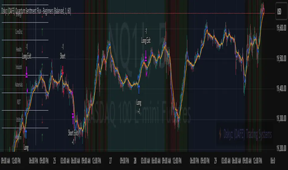
Long/ Short with Big Trend v1.0-strategyHello traders,
This script using multi MA and EMA , MACD , RSI ... for vote BUY or SELL.
If 80% signal vote for BUY, signal Long will been active
or 80% signal vote for SELL, signal Short will been active
Recommend using this script for Trend trader, not using for Scalping trader or Swing trader!
Best backtest in:
- BTC/USDT H8, D1
- LTC/USDT: D1
- ETH/USDT: H8
- BCH/USDT: H2, H4
- LINK/USDT: H8
...
With other symbols and time frame, you can do it yourself.
We are recommend using with min time frame H2 for all symbol or using H8 only.
Setting for backtest:
- Signal %: set percent for active signal. Recommend set 80 for big time frame or 90-95 for small time frame.
- Trade type:
+ LongShort (default): trade Long and Short if you trade with margin account.
+ LongOnly: if you trade with spot account, select Long only for backtest.
+ ShortOnly: if you trade with margin account and like short only.
- Take profit %: close order if profit > this value. Set to 0 for disable this function.
- Stop loss %: close order if profit < this value. Set to 0 for disable this function.
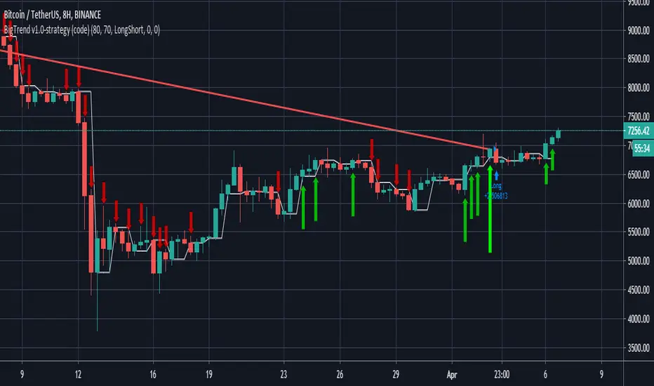
THE PHOENIX v0.1 wSMDAS requested - Version of my Phoenix Script with both LONG and SHORTS, Backtest results will not be accurate unless you use margin trading.
------------------------------------------------------------------------------------------------------------------------------------------------------------------------------------
Implementation in TradingView of modified version of the "Weis Wave".
indicatior will generate Long and Close Long signals according to market trend.
(Learned the hard way that using short instead of close long to close long orders will seriously mess backtest results and create unrealistic expectations)
Added a customizable RATE OF CHANGE indicator that I called SMD (sideways market detection) to try and avoid trading on sideways market.
References: "Trades About To Happen" David H. Weis, Division 2 of the Richard D. Wyckoff Method of Trading in Stocks.
I've had best results on 2h and 4h charts, I would not recommend to go below 1h, my general rule is to run the backtest on regular candle and make sure the backtest gives goodd result, but I use the script with autoview on heikin ashi.
Backtesting: You can change the dates of the backtest as you please, the backtest runs with 1000USD and 100% of equity orders, 3 ticks slippage and 0.1% commission.
For Autoview users: Will upload LONG ALERT and CLOSE LONG ALERT studies separately as I find it easier to see whats going on on 2 seperate indicators.
NO, IT DOES NOT REPAINT.
