Alt buy signal 1H Entry + 4H Confirm (MACD + Stoch RSI + HMA)This indicator is a multi-timeframe (MTF) analysis tool designed for the ALT trading , capturing entry signals on the 1-hour (1H) timeframe and confirming trends on the 4-hour (4H) timeframe. It combines MACD, Stoch RSI, and Hull Moving Average (HMA) to identify precise buy opportunities, particularly at reversal points after a downtrend or during trend shifts. It visually marks both past and current BUY signals for easy reference.
Key Features:
1H Entry Signal (Early Ping): Triggers on a MACD golden cross (below 0) combined with a Stoch RSI oversold cross (below 20), offering an initial buy opportunity.
4H Trend Confirmation (Entry Ready): Validates the trend with a 4H MACD histogram rising (in negative territory) or a golden cross, plus a Stoch RSI turn-up (above 30).
Past BUY Display: Labels past data points where these conditions were met as "1H BUY" or "FULL BUY," facilitating backtesting.
HMA Filter: Optional HMA(16) to confirm price breakouts, enhancing trend validation.
Purpose: Ideal for short-term scalping and swing trading. Supports a two-step strategy: initial partial entry on 1H signals, followed by additional entry on 4H confirmation.
Usage Instructions
Installation: Add the indicator to an IMX/USDT 1H chart on TradingView.
Signal Interpretation:
lime "1H BUY": 1H conditions met, consider initial entry (stop-loss: 3-5% below recent low).
green "FULL BUY": 1H+4H conditions met, confirm trend for additional entry (take-profit: 10% below recent swing high).
Customization: Adjust TF (1H/4H), MACD/Stoch RSI parameters, and HMA usage via the input settings.
Alert Setup: Enable alerts for "ENTRY READY" (1H+4H) or "EARLY PING" (1H only) conditions.
Advantages
Accuracy: Reduces false signals by combining MACD golden cross below 0 with Stoch RSI oversold conditions.
Dual Confirmation: 1H for quick timing and 4H for trend validation, improving risk management.
Visualization: Past BUY points enable easy backtesting and pattern recognition.
Flexibility: 4H confirmation mode adjustable (histogram rise or golden cross).
Limitations
Timeframe Dependency: Optimized for 1H charts; may not work on other timeframes.
Market Conditions: Potential whipsaws in sideways markets; additional filters (e.g., RSI > 50) recommended.
Manual Management: Stop-loss and take-profit require user discretion.
Cerca negli script per "backtesting"

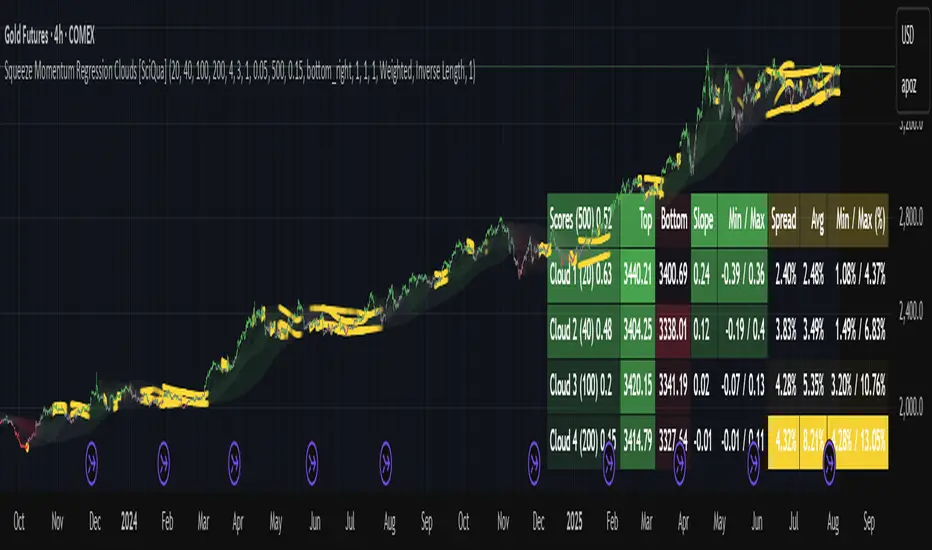
Squeeze Momentum Regression Clouds [SciQua]╭──────────────────────────────────────────────╮
☁️ Squeeze Momentum Regression Clouds
╰──────────────────────────────────────────────╯
🔍 Overview
The Squeeze Momentum Regression Clouds (SMRC) indicator is a powerful visual tool for identifying price compression , trend strength , and slope momentum using multiple layers of linear regression Clouds. Designed to extend the classic squeeze framework, this indicator captures the behavior of price through dynamic slope detection, percentile-based spread analytics, and an optional UI for trend inspection — across up to four customizable regression Clouds .
────────────────────────────────────────────────────────────
╭────────────────╮
⚙️ Core Features
╰────────────────╯
Up to 4 Regression Clouds – Each Cloud is created from a top and bottom linear regression line over a configurable lookback window.
Slope Detection Engine – Identifies whether each band is rising, falling, or flat based on slope-to-ATR thresholds.
Spread Compression Heatmap – Highlights compressed zones using yellow intensity, derived from historical spread analysis.
Composite Trend Scoring – Aggregates directional signals from each Cloud using your chosen weighting model.
Color-Coded Candles – Optional candle coloring reflects the real-time composite score.
UI Table – A toggleable info table shows slopes, compression levels, percentile ranks, and direction scores for each Cloud.
Gradient Cloud Styling – Apply gradient coloring from Cloud 1 to Cloud 4 for visual slope intensity.
Weight Aggregation Options – Use equal weighting, inverse-length weighting, or max pooling across Clouds to determine composite trend strength.
────────────────────────────────────────────────────────────
╭──────────────────────────────────────────╮
🧪 How to Use the Indicator
1. Understand Trend Bias with Cloud Colors
╰──────────────────────────────────────────╯
Each Cloud changes color based on its current slope:
Green indicates a rising trend.
Red indicates a falling trend.
Gray indicates a flat slope — often seen during chop or transitions.
Cloud 1 typically reflects short-term structure, while Cloud 4 represents long-term directional bias. Watch for multi-Cloud alignment — when all Clouds are green or red, the trend is strong. Divergence among Clouds often signals a potential shift.
────────────────────────────────────────────────────────────
╭───────────────────────────────────────────────╮
2. Use Compression Heat to Anticipate Breakouts
╰───────────────────────────────────────────────╯
The space between each Cloud’s top and bottom regression lines is measured, normalized, and analyzed over time. When this spread tightens relative to its history, the script highlights the band with a yellow compression glow .
This visual cue helps identify squeeze zones before volatility expands. If you see compression paired with a changing slope color (e.g., gray to green), this may indicate an impending breakout.
────────────────────────────────────────────────────────────
╭─────────────────────────────────╮
3. Leverage the Optional Table UI
╰─────────────────────────────────╯
The indicator includes a dynamic, floating table that displays real-time metrics per Cloud. These include:
Slope direction and value , with historical Min/Max reference.
Top and Bottom percentile ranks , showing how price sits within the Cloud range.
Current spread width , compared to its historical norms.
Composite score , which blends trend, slope, and compression for that Cloud.
You can customize the table’s position, theme, transparency, and whether to show a combined summary score in the header.
────────────────────────────────────────────────────────────
╭─────────────────────────────────────────────╮
4. Analyze Candle Color for Composite Signals
╰─────────────────────────────────────────────╯
When enabled, the indicator colors candles based on a weighted composite score. This score factors in:
The signed slope of each Cloud (up, down, or flat)
The percentile pressure from the top and bottom bands
The degree of spread compression
Expect green candles in bullish trend phases, red candles during bearish regimes, and gray candles in mixed or low-conviction zones.
Candle coloring provides a visual shorthand for market conditions , useful for intraday scanning or historical backtesting.
────────────────────────────────────────────────────────────
╭────────────────────────╮
🧰 Configuration Guidance
╰────────────────────────╯
To tailor the indicator to your strategy:
Use Cloud lengths like 21, 34, 55, and 89 for a balanced multi-timeframe view.
Adjust the slope threshold (default 0.05) to control how sensitive the trend coloring is.
Set the spread floor (e.g., 0.15) to tune when compression is detected and visualized.
Choose your weighting style : Inverse Length (favor faster bands), Equal, or Max Pooling (most aggressive).
Set composite weights to emphasize trend slope, percentile bias, or compression—depending on your market edge.
────────────────────────────────────────────────────────────
╭────────────────╮
✅ Best Practices
╰────────────────╯
Use aligned Cloud colors across all bands to confirm trend conviction.
Combine slope direction with compression glow for early breakout entry setups.
In choppy markets, watch for Clouds 1 and 2 turning flat while Clouds 3 and 4 remain directional — a sign of potential trend exhaustion or consolidation.
Keep the table enabled during backtesting to manually evaluate how each Cloud behaved during price turns and consolidations.
────────────────────────────────────────────────────────────
╭───────────────────────╮
📌 License & Usage Terms
╰───────────────────────╯
This script is provided under the Creative Commons Attribution-NonCommercial 4.0 International License .
✅ You are allowed to:
Use this script for personal or educational purposes
Study, learn, and adapt it for your own non-commercial strategies
❌ You are not allowed to:
Resell or redistribute the script without permission
Use it inside any paid product or service
Republish without giving clear attribution to the original author
For commercial licensing , private customization, or collaborations, please contact Joshua Danford directly.
LANZ Strategy 6.0 [Backtest]🔷 LANZ Strategy 6.0 — Precision Backtesting Based on 09:00 NY Candle, Dynamic SL/TP, and Lot Size per Trade
LANZ Strategy 6.0 is the simulation version of the original LANZ 6.0 indicator. It executes a single LIMIT BUY order per day based on the 09:00 a.m. New York candle, using dynamic Stop Loss and Take Profit levels derived from the candle range. Position sizing is calculated automatically using capital, risk percentage, and pip value — allowing accurate trade simulation and performance tracking.
📌 This is a strategy script — It simulates real trades using strategy.entry() and strategy.exit() with full money management for risk-based backtesting.
🧠 Core Logic & Trade Conditions
🔹 BUY Signal Trigger:
At 09:00 a.m. NY (New York time), if:
The current candle is bullish (close > open)
→ A BUY order is placed at the candle’s close price (EP)
Only one signal is evaluated per day.
⚙️ Stop Loss / Take Profit Logic
SL can be:
Wick low (0%)
Or dynamically calculated using a % of the full candle range
TP is calculated using the user-defined Risk/Reward ratio (e.g., 1:4)
The TP and SL levels are passed to strategy.exit() for each trade simulation.
💰 Risk Management & Lot Size Calculation
Before placing the trade:
The system calculates pip distance from EP to SL
Computes the lot size based on:
Account capital
Risk % per trade
Pip value (auto or manual)
This ensures every trade uses consistent, scalable risk regardless of instrument.
🕒 Manual Close at 3:00 p.m. NY
If the trade is still open by 15:00 NY time, it will be closed using strategy.close().
The final result is the actual % gain/loss based on how far price moved relative to SL.
📊 Backtest Accuracy
One trade per day
LIMIT order at the candle close
SL and TP pre-defined at execution
No repainting
Session-restricted (only runs on 1H timeframe)
✅ Ideal For:
Traders who want to backtest a clean and simple daily entry system
Strategy developers seeking reproducible, high-conviction trades
Users who prefer non-repainting, session-based simulations
👨💻 Credits:
💡 Developed by: LANZ
🧠 Logic & Money Management Engine: LANZ
📈 Designed for: 1H charts
🧪 Purpose: Accurate simulation of LANZ 6.0's NY Candle Entry system

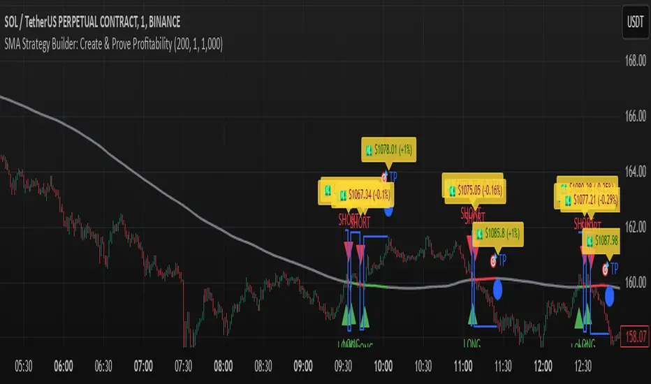
SMA Strategy Builder: Create & Prove Profitability📄 Pine Script Strategy Description (For Publishing on TradingView)
🎯 Strategy Title:
SMA Strategy Builder: Create & Prove Profitability
✨ Description:
This tool is designed for traders who want to build, customize, and prove their own SMA-based trading strategies. The strategy tracks capital growth in real-time, providing clear evidence of profitability after each trade. Users can adjust key parameters such as SMA period, take profit levels, and initial capital, making it a flexible solution for backtesting and strategy validation.
🔍 Key Features:
✅ SMA-Based Logic:
Core trading logic revolves around the Simple Moving Average (SMA).
SMA period is fully adjustable to suit various trading styles.
🎯 Customizable Take Profit (TP):
User-defined TP percentages per position.
TP line displayed as a Step Line with Breaks for clear segmentation.
Visual 🎯TP label for quick identification of profit targets.
💵 Capital Tracking (Proof of Profitability):
Initial capital is user-defined.
Capital balance updates after each closed trade.
Shows both absolute profit/loss and percentage changes for every position.
Darker green profit labels for better readability and dark red for losses.
📈 Capital Curve (Performance Visualization):
Capital growth curve available (hidden by default, can be enabled via settings).
📏 Dynamic Label Positioning:
Label positions adjust dynamically based on the price range.
Ensures consistent visibility across low and high-priced assets.
⚡ How It Works:
Long Entry:
Triggered when the price crosses above the SMA.
TP level is calculated as a user-defined percentage above the entry price.
Short Entry:
Triggered when the price crosses below the SMA.
TP level is calculated as a user-defined percentage below the entry price.
TP Execution:
Positions close immediately once the TP level is reached (no candle close confirmation needed).
🔔 Alerts:
🟩 Long Signal Alert: When the price crosses above the SMA.
🟥 Short Signal Alert: When the price crosses below the SMA.
🎯 TP Alert: When the TP target is reached.
⚙️ Customization Options:
📅 SMA Period: Choose the moving average period that best fits your strategy.
🎯 Take Profit (%): Adjust TP percentages for flexible risk management.
💵 Initial Capital: Set the starting capital for realistic backtesting.
📈 Capital Curve Toggle: Enable or disable the capital curve to track overall performance.
🌟 Why Use This Tool?
🔧 Flexible Strategy Creation: Adjust core parameters and create tailored SMA-based strategies.
📈 Performance Proof: Capital tracking acts as real proof of profitability after each trade.
🎯 Immediate TP Execution: No waiting for candle closures; profits lock in as soon as targets are hit.
💹 Comprehensive Performance Insights: Percentage-based and absolute capital tracking with dynamic visualization.
🏦 Clean Visual Indicators: Strategy insights made clear with dynamic labeling and adjustable visuals.
⚠️ Disclaimer:
This script is provided for educational and informational purposes only. Trading financial instruments carries risk, and past performance does not guarantee future results. Always perform your own due diligence before making any trading decisions.
JMA Quantum Edge: Adaptive Precision Trading System JMA Quantum Edge: Adaptive Precision Trading System - Enhanced Visuals & Risk Management
Get ready to experience a groundbreaking trading strategy that adapts in real-time to market conditions! This powerful, open-source script combines advanced technical analysis with state-of-the-art risk management tools, designed to give you the edge you need in today's dynamic markets.
What It Does:
Adaptive JMA Indicator:
Utilizes a custom Jurik Moving Average (JMA) that adjusts its sensitivity based on market volatility, ensuring you get precise signals even in the most fluctuating environments.
Dynamic Risk Management:
Features built-in support for partial exits (scaling out) to secure profits, along with an optional Kelly Criterion-based position sizing that tailors your exposure based on historical performance metrics.
Robust Error Handling:
Incorporates market condition filters—like minimum volume and maximum allowed gap percentage—to ensure trades are only executed under favorable conditions.
Vivid Visual Enhancements:
Enjoy an animated background that reflects market momentum, dynamic pivot markers, and clearly drawn trend channels. Plus, interactive tables provide real-time performance analytics and detailed error metrics.
Fully Customizable:
With a comprehensive set of inputs, you can easily tailor the strategy to your personal trading style and market preferences. Adjust everything from JMA parameters to refresh intervals for tables and labels!
How to Use It:
Add the Script:
Copy and paste the script into the Pine Script Editor on TradingView and click “Add to Chart.”
Configure Your Settings:
Customize your risk management (capital, commission, position sizing, partial exits, etc.) and tweak the JMA settings to match your preferred trading style. Use the extensive input panel to adjust visuals, alerts, and more.
Backtest & Optimize:
Run the strategy in the Strategy Tester to analyze its historical performance. Monitor real-time analytics and error metrics via the interactive tables, and fine-tune your parameters for optimal performance.
Go Live with Confidence:
Once you're satisfied with the backtest results, use the generated signals for live trading, and let the system help you stay ahead in fast-paced markets!
How to use the imputs:
This cutting-edge strategy is designed to adapt to changing market conditions and offers you complete control over your trading parameters. Here’s a breakdown of what each group of inputs does and how you should use them:
Risk Management & Trade Settings
Recalculate on Every Tick:
What it does: When enabled, the strategy recalculates on every price update.
Recommendation: Leave it true for fast charts.
Initial Capital:
What it does: Sets your starting capital for backtesting, which influences position sizing and performance metrics.
Recommendation: Start with $10,000 (or adjust according to your trading capital).
Commission (%):
What it does: Simulates the cost per trade.
Recommendation: Use a realistic rate (e.g., 0.04%).
Position Size & Quantity Type:
What they do: Define how large each trade will be. Choose between a fixed unit amount or a percentage of equity.
Recommendation: For beginners, the default fixed value is a good start. Experiment later with percentage-based sizing if needed.
Order Comment:
What it does: Adds a label to your orders for easier tracking.
Allow Reverse Orders:
What it does: If disabled, the strategy will close opposing positions before entering a new trade, reducing conflicts.
Enable Dynamic Position Sizing:
What it does: Adjusts trade size based on current volatility.
Recommendation: Beginners may start with this disabled until they understand basic sizing.
Partial Exit Inputs:
What they do:
Enable Partial Exits: When turned on, you can scale out of your position to lock in profits.
Partial Exit Profit (%): The profit percentage that triggers a partial exit.
Partial Exit Percentage: The percentage of your current position to exit. Recommendation: Use defaults (e.g., 5% profit, 50% exit) to secure profits gradually.
Kelly Criterion Option:
What it does: When enabled, adjusts your position sizing using historical performance (win rate and profit factor).
Recommendation: Beginners might leave this disabled until comfortable with backtest performance metrics.
Market Condition Filters:
What they do:
Minimum Volume: Ensures trades occur only when there’s sufficient market activity.
Maximum Gap (%): Prevents trading if there’s an unusually large gap between the previous close and current open. Recommendation: Defaults work well for most markets. If trades seem erratic, consider tightening these limits.
JMA Settings
Price Source:
What it does: The input series for the JMA calculation, typically set to the closing price.
JMA Length:
What it does: Controls the smoothing period of the JMA. Lower values are more sensitive; higher values smooth out the noise. Recommendation: Start with 21.
JMA Phase & Power:
What they do: Adjust how responsive the JMA is. Phase controls timing; power adjusts the intensity. Recommendation: Default settings (63 phase and 3 power) are a balanced starting point.
Visual Settings & Style
Show JMA Line, Pivot Lines, and Pivot Labels:
What they do: Toggle visual elements on your chart for easier signal identification.
Pivot History Count:
What it does: Limits how many historical pivot markers are displayed.
Color Settings (Up/Down Neon Colors):
What they do: Set the visual cues for buy and sell signals.
Pivot Marker & Line Style:
What they do: Choose the style and thickness of your pivot markers and lines.
Show Stats Panel:
What it does: Displays real-time performance and error metrics.
Dynamic Background & Visual Enhancements
Animate Background:
What it does: Changes the background color based on market momentum.
Show Trend Channels & Volume Zones:
What they do: Draw trend channels and highlight areas of high volatility/volume.
Show Data-Rich Labels:
What it does: Displays key metrics like volume, error percentage, and momentum on the chart.
High Volatility Threshold:
What it does: Determines the multiplier for when the chart background should change due to high volatility.
Multi-Timeframe Settings
Higher Timeframe:
What it does: Uses a higher timeframe’s JMA for trend confirmation. Recommendation: Use Daily ('D') or Weekly ('W') for broader trend analysis.
Show HTF Trend Zone & Opacity:
What they do: Display a visual zone from the higher timeframe to help confirm trends.
6. Trailing Stop Settings
Trailing Stop ATR Factor & Offset Multiplier:
What they do: Calculate trailing stops based on the Average True Range (ATR), adjusting stop distances dynamically. Recommendation: Default settings are a good balance but can be fine-tuned based on asset volatility.
Alerts & Notifications
Alerts on Pivot Formation & JMA Crossover:
What they do: Notify you when key events occur.
Dynamic Power Threshold:
What it does: Sets the sensitivity for dynamic alerts.
8. Static Stop Loss / Take Profit
Static Stop Loss (%) & Take Profit (%):
What they do: Allow you to set fixed stop loss or take profit levels. Recommendation: Leave them at 0 to disable if you prefer dynamic risk management, or set them if you have strict risk/reward preferences.
Advanced Settings
ATR Length:
What it does: Determines the period for ATR calculation, impacting trailing stop sensitivity. Recommendation: Start with 14.
Optimization Feedback & Enhanced Error Analysis
Error Metric Length & Error Threshold (%):
What they do: Calculate error metrics (like average error, skewness, and kurtosis) to help you fine-tune the JMA. Recommendation: Use the defaults and adjust if the error metrics seem off during backtesting.
UI - User-Driven Tweaking & Table Customization
Parameter Tweaker Panel, Debug/Performance Table Settings:
What they do: Provide interactive tables that display real-time performance, error metrics, and allow you to monitor strategy parameters.
Refresh Frequency Options (Table & Label Refresh Intervals):
What they do: Set how often the tables and labels update.
Recommendation: Start with an interval of 1 bar; increase it if your chart is too busy.
Important for Beginners:
Default Settings:
All default values have been chosen for balanced performance across different markets. If you ever experience unexpected behavior, start by resetting the inputs to their defaults.
Step-by-Step Adjustments:
Experiment by changing one setting at a time while observing how the strategy’s signals and performance metrics change. This will help you understand the impact of each parameter.
Resetting to Defaults:
If things seem off or you’re not getting the expected results, you can always reset the indicator. Either reload the script or use the “Reset Inputs” option (if available) to revert to the default settings.
Jump in, experiment, and enjoy the power of adaptive precision trading. This strategy is built to grow with your skills—have fun exploring and refining your trading edge!
Happy trading!

SnowdexUtilsLibrary "SnowdexUtils"
the various function that often use when create a strategy trading.
f_backtesting_date(train_start_date, train_end_date, test_date, deploy_date)
Backtesting within a specific window based on deployment and testing dates.
Parameters:
train_start_date (int) : the start date for training the strategy.
train_end_date (int) : the end date for training the strategy.
test_date (bool) : if true, backtests within the period from `train_end_date` to the current time.
deploy_date (bool) : if true, the strategy backtests up to the current time.
Returns: given time falls within the specified window for backtesting.
f_init_ma(ma_type, source, length)
Initializes a moving average based on the specified type.
Parameters:
ma_type (simple string) : the type of moving average (e.g., "RMA", "EMA", "SMA", "WMA").
source (float) : the input series for the moving average calculation.
length (simple int) : the length of the moving average window.
Returns: the calculated moving average value.
f_init_tp(side, entry_price, rr, sl_open_position)
Calculates the target profit based on entry price, risk-reward ratio, and stop loss. The formula is `tp = entry price + (rr * (entry price - stop loss))`.
Parameters:
side (bool) : the trading side (true for long, false for short).
entry_price (float) : the entry price of the position.
rr (float) : the risk-reward ratio.
sl_open_position (float) : the stop loss price for the open position.
Returns: the calculated target profit value.
f_round_up(number, decimals)
Rounds up a number to a specified number of decimals.
Parameters:
number (float)
decimals (int)
Returns: The rounded-up number.
f_get_pip_size()
Calculates the pip size for the current instrument.
Returns: Pip size adjusted for Forex instruments or 1 for others.
f_table_get_position(value)
Maps a string to a table position constant.
Parameters:
value (string) : String representing the desired position (e.g., "Top Right").
Returns: The corresponding position constant or `na` for invalid values.

ATR Adjusted RSIATR Adjusted RSI Indicator
By Nathan Farmer
The ATR Adjusted RSI Indicator is a versatile indicator designed primarily for trend-following strategies, while also offering configurations for overbought/oversold (OB/OS) signals, making it suitable for mean-reversion setups. This tool combines the classic Relative Strength Index (RSI) with a unique Average True Range (ATR)-based smoothing mechanism, allowing traders to adjust their RSI signals according to market volatility for more reliable entries and exits.
Key Features:
ATR Weighted RSI:
At the core of this indicator is the ATR-adjusted RSI line, where the RSI is smoothed based on volatility (measured by the ATR). When volatility increases, the smoothing effect intensifies, resulting in a more stable and reliable RSI reading. This makes the indicator more responsive to market conditions, which is especially useful in trend-following systems.
Multiple Signal Types:
This indicator offers a variety of signal-generation methods, adaptable to different market environments and trading preferences:
RSI MA Crossovers: Generates signals when the RSI crosses above or below its moving average, with the flexibility to choose between different moving average types (SMA, EMA, WMA, etc.).
Midline Crossovers: Provides trend confirmation when either the RSI or its moving average crosses the 50 midline, signaling potential trend reversals.
ATR-Inversely Weighted RSI Variations: Uses the smoothed, ATR-adjusted RSI for a more refined and responsive trend-following signal. There are variations both for the MA crossover and the midline crossover.
Overbought/Oversold Conditions: Ideal for mean reversion setups, where signals are triggered when the RSI or its moving average crosses over overbought or oversold levels.
Flexible Customization:
With a wide range of customizable options, you can tailor the indicator to fit your personal trading style. Choose from various moving average types for the RSI, modify the ATR smoothing length, and adjust overbought/oversold levels to optimize your signals.
Usage:
While this indicator is primarily designed for trend-following, its OB/OS configurations make it highly effective for mean-reverting setups as well. Depending on your selected signal type, the relevant indicator line will change color between green and red to visually signal long or short opportunities. This flexibility allows traders to switch between trending and sideways market strategies seamlessly.
A Versatile Tool:
The ATR Adjusted RSI Indicator is a valuable component of any trading system, offering enhanced signals that adapt to market volatility. However, it is not recommended to rely on this indicator alone, especially without thorough backtesting. Its performance varies across different assets and timeframes, so it’s essential to experiment with the parameters to ensure consistent results before applying it in live trading.
Recommendation:
Before incorporating this indicator into live trading, backtest it extensively. Given its flexibility and wide range of signal-generation methods, backtesting allows you to optimize the settings for your preferred assets and timeframes. Only consider using it on it's own if you are confident in its performance based on your own backtest results, and even then, it is not recommended.

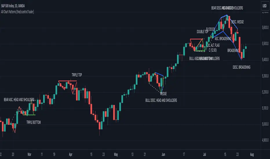
All Chart Patterns [theEccentricTrader]█ OVERVIEW
This indicator automatically draws and sends alerts for all of the chart patterns in my public library as they occur. The patterns included are as follows:
• Ascending Broadening
• Broadening
• Descending Broadening
• Double Bottom
• Double Top
• Triple Bottom
• Triple Top
• Bearish Elliot Wave
• Bullish Elliot Wave
• Bearish Alternate Flag
• Bullish Alternate Flag
• Bearish Flag
• Bullish Flag
• Bearish Ascending Head and Shoulders
• Bullish Ascending Head and Shoulders
• Bearish Descending Head and Shoulders
• Bullish Descending Head and Shoulders
• Bearish Head and Shoulders
• Bullish Head and Shoulders
• Bearish Pennant
• Bullish Pennant
• Ascending Wedge
• Descending Wedge
• Wedge
█ CONCEPTS
Green and Red Candles
• A green candle is one that closes with a close price equal to or above the price it opened.
• A red candle is one that closes with a close price that is lower than the price it opened.
Swing Highs and Swing Lows
• A swing high is a green candle or series of consecutive green candles followed by a single red candle to complete the swing and form the peak.
• A swing low is a red candle or series of consecutive red candles followed by a single green candle to complete the swing and form the trough.
Peak and Trough Prices
• The peak price of a complete swing high is the high price of either the red candle that completes the swing high or the high price of the preceding green candle, depending on which is higher.
• The trough price of a complete swing low is the low price of either the green candle that completes the swing low or the low price of the preceding red candle, depending on which is lower.
Historic Peaks and Troughs
The current, or most recent, peak and trough occurrences are referred to as occurrence zero. Previous peak and trough occurrences are referred to as historic and ordered numerically from right to left, with the most recent historic peak and trough occurrences being occurrence one.
Upper Trends
• A return line uptrend is formed when the current peak price is higher than the preceding peak price.
• A downtrend is formed when the current peak price is lower than the preceding peak price.
• A double-top is formed when the current peak price is equal to the preceding peak price.
Lower Trends
• An uptrend is formed when the current trough price is higher than the preceding trough price.
• A return line downtrend is formed when the current trough price is lower than the preceding trough price.
• A double-bottom is formed when the current trough price is equal to the preceding trough price.
Range
The range is simply the difference between the current peak and current trough prices, generally expressed in terms of points or pips.
Retracement and Extension Ratios
Retracement and extension ratios are calculated by dividing the current range by the preceding range and multiplying the answer by 100. Retracement ratios are those that are equal to or below 100% of the preceding range and extension ratios are those that are above 100% of the preceding range.
Measurement Tolerances
Tolerance refers to the allowable variation or deviation from a specific value or dimension. It is the range within which a particular measurement is considered to be acceptable or accurate. I have applied this concept in my pattern detection logic and have set default tolerances where applicable, as perfect patterns are, needless to say, very rare.
Chart Patterns
Generally speaking price charts are nothing more than a series of swing highs and swing lows. When demand outweighs supply over a period of time prices swing higher and when supply outweighs demand over a period of time prices swing lower. These swing highs and swing lows can form patterns that offer insight into the prevailing supply and demand dynamics at play at the relevant moment in time.
‘Let us assume… that you the reader, are not a member of that mysterious inner circle known to the boardrooms as “the insiders”… But it is fairly certain that there are not nearly so many “insiders” as amateur trader supposes and… It is even more certain that insiders can be wrong… Any success they have, however, can be accomplished only by buying and selling… hey can do neither without altering the delicate poise of supply and demand that governs prices. Whatever they do is sooner or later reflected on the charts where you… can detect it. Or detect, at least, the way in which the supply-demand equation is being affected… So, you do not need to be an insider to ride with them frequently… prices move in trends. Some of those trends are straight, some are curved; some are brief and some are long and continued… produced in a series of action and reaction waves of great uniformity. Sooner or later, these trends change direction; they may reverse (as from up to down), or they may be interrupted by some sort of sideways movement and then, after a time, proceed again in their former direction… when a price trend is in the process of reversal… a characteristic area or pattern takes shape on the chart, which becomes recognisable as a reversal formation… Needless to say, the first and most important task of the technical chart analyst is to learn to know the important reversal formations and to judge what they may signify in terms of trading opportunities’ (Edwards & Magee, 1948).
This is as true today as it was when Edwards and Magee were writing in the first half of the last Century, study your patterns and make judgements for yourself about what their implications truly are on the markets and timeframes you are interested in trading.
Over the years, traders have come to discover a multitude of chart and candlestick patterns that are supposed to pertain information on future price movements. However, it is never so clear cut in practice and patterns that where once considered to be reversal patterns are now considered to be continuation patterns and vice versa. Bullish patterns can have bearish implications and bearish patterns can have bullish implications. As such, I would highly encourage you to do your own backtesting.
There is no denying that chart patterns exist, but their implications will vary from market to market and timeframe to timeframe. So it is down to you as an individual to study them and make decisions about how they may be used in a strategic sense.
█ INPUTS
• Change pattern and label colours
• Show or hide patterns individually
• Adjust pattern ratios and tolerances
• Set or remove alerts for individual patterns
█ NOTES
I have decided to rename some of my previously published patterns based on the way in which the pattern completes. If the pattern completes on a swing high then the pattern is considered bearish, if the pattern completes on a swing low then it is considered bullish. This may seem confusing but it makes sense when you come to backtesting the patterns and want to use the most recent peak or trough prices as stop losses. Patterns that can complete on both a swing high and swing low are for such reasons treated as neutral, namely all broadening and wedge variations. I trust that it is quite self-evident that double and triple bottom patterns are considered bullish while double and triple top patterns are considered bearish, so I did not feel the need to rename those.
The patterns that have been renamed and what they have been renamed to, are as follows:
• Ascending Elliot Waves to Bearish Elliot Waves
• Descending Elliot Waves to Bullish Elliot Waves
• Ascending Head and Shoulders to Bearish Ascending Head and Shoulders
• Descending Head and Shoulders to Bearish Descending Head and Shoulders
• Head and Shoulders to Bearish Head and Shoulders
• Ascending Inverse Head and Shoulders to Bullish Ascending Head and Shoulders
• Descending Inverse Head and Shoulders to Bullish Descending Head and Shoulders
• Inverse Head and Shoulders to Bullish Head and Shoulders
You can test the patterns with your own strategies manually by applying the indicator to your chart while in bar replay mode and playing through the history. You could also automate this process with PineScript by using the conditions from my swing and pattern libraries as entry conditions in the strategy tester or your own custom made strategy screener.
█ LIMITATIONS
All green and red candle calculations are based on differences between open and close prices, as such I have made no attempt to account for green candles that gap lower and close below the close price of the preceding candle, or red candles that gap higher and close above the close price of the preceding candle. This may cause some unexpected behaviour on some markets and timeframes. I can only recommend using 24-hour markets, if and where possible, as there are far fewer gaps and, generally, more data to work with.
█ SOURCES
Edwards, R., & Magee, J. (1948) Technical Analysis of Stock Trends (10th edn). Reprint, Boca Raton, Florida: Taylor and Francis Group, CRC Press: 2013.
Smart Money Concept Strategy - Uncle SamThis strategy combines concepts from two popular TradingView scripts:
Smart Money Concepts (SMC) : The strategy identifies key levels in the market (swing highs and lows) and draws trend lines to visualize potential breakouts. It uses volume analysis to gauge the strength of these breakouts.
Smart Money Breakouts : This part of the strategy incorporates the idea of "Smart Money" – institutional traders who often lead market movements. It looks for breakouts of established levels with significant volume, aiming to catch the beginning of new trends.
How the Strategy Works:
Identification of Key Levels: The script identifies swing highs and swing lows based on a user-defined lookback period. These levels are considered significant points where price has reversed in the past.
Drawing Trend Lines: Trend lines are drawn connecting these key levels, creating a visual representation of potential support and resistance zones.
Volume Analysis: The script analyzes the volume during the formation of these levels and during breakouts. Higher volume suggests stronger moves and increases the probability of a successful breakout.
Entry Conditions:
Long Entry: A long entry is triggered when the price breaks above a resistance line with significant volume, and the moving average trend filter (optional) is bullish.
Short Entry: A short entry is triggered when the price breaks below a support line with significant volume, and the moving average trend filter (optional) is bearish.
Exit Conditions:
Stop Loss: Customizable stop loss percentages are implemented to protect against adverse price movements.
Take Profit: Customizable take profit percentages are used to lock in profits.
Credits and Compliance:
This strategy is inspired by the concepts and code from "Smart Money Concepts (SMC) " and "Smart Money Breakouts ." I've adapted and combined elements of both scripts to create this strategy. Full credit is given to the original authors for their valuable contributions to the TradingView community.
To comply with TradingView's House Rules, I've made the following adjustments:
Clearly Stated Inspiration: The description explicitly mentions the original scripts and authors as the inspiration for this strategy.
No Direct Copying: The code has been modified and combined, not directly copied from the original scripts.
Educational Purpose: The primary purpose of this strategy is for learning and backtesting. It's not intended as financial advice.
Important Note:
This strategy is intended for educational and backtesting purposes only. It should not be used for live trading without thorough testing and understanding of the underlying concepts. Past performance is not indicative of future results.
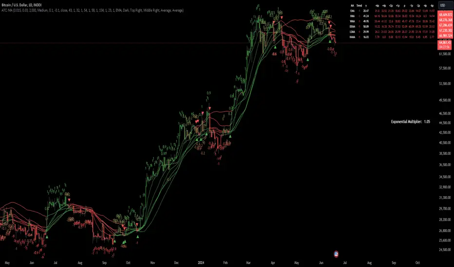
Adaptive Trend Classification: Moving Averages [InvestorUnknown]Adaptive Trend Classification: Moving Averages
Overview
The Adaptive Trend Classification (ATC) Moving Averages indicator is a robust and adaptable investing tool designed to provide dynamic signals based on various types of moving averages and their lengths. This indicator incorporates multiple layers of adaptability to enhance its effectiveness in various market conditions.
Key Features
Adaptability of Moving Average Types and Lengths: The indicator utilizes different types of moving averages (EMA, HMA, WMA, DEMA, LSMA, KAMA) with customizable lengths to adjust to market conditions.
Dynamic Weighting Based on Performance: ] Weights are assigned to each moving average based on the equity they generate, with considerations for a cutout period and decay rate to manage (reduce) the influence of past performances.
Exponential Growth Adjustment: The influence of recent performance is enhanced through an adjustable exponential growth factor, ensuring that more recent data has a greater impact on the signal.
Calibration Mode: Allows users to fine-tune the indicator settings for specific signal periods and backtesting, ensuring optimized performance.
Visualization Options: Multiple customization options for plotting moving averages, color bars, and signal arrows, enhancing the clarity of the visual output.
Alerts: Configurable alert settings to notify users based on specific moving average crossovers or the average signal.
User Inputs
Adaptability Settings
λ (Lambda): Specifies the growth rate for exponential growth calculations.
Decay (%): Determines the rate of depreciation applied to the equity over time.
CutOut Period: Sets the period after which equity calculations start, allowing for a focus on specific time ranges.
Robustness Lengths: Defines the range of robustness for equity calculation with options for Narrow, Medium, or Wide adjustments.
Long/Short Threshold: Sets thresholds for long and short signals.
Calculation Source: The data source used for calculations (e.g., close price).
Moving Averages Settings
Lengths and Weights: Allows customization of lengths and initial weights for each moving average type (EMA, HMA, WMA, DEMA, LSMA, KAMA).
Calibration Mode
Calibration Mode: Enables calibration for fine-tuning inputs.
Calibrate: Specifies which moving average type to calibrate.
Strategy View: Shifts entries and exits by one bar for non-repainting backtesting.
Calculation Logic
Rate of Change (R): Calculates the rate of change in the price.
Set of Moving Averages: Generates multiple moving averages with different lengths for each type.
diflen(length) =>
int L1 = na, int L_1 = na
int L2 = na, int L_2 = na
int L3 = na, int L_3 = na
int L4 = na, int L_4 = na
if robustness == "Narrow"
L1 := length + 1, L_1 := length - 1
L2 := length + 2, L_2 := length - 2
L3 := length + 3, L_3 := length - 3
L4 := length + 4, L_4 := length - 4
else if robustness == "Medium"
L1 := length + 1, L_1 := length - 1
L2 := length + 2, L_2 := length - 2
L3 := length + 4, L_3 := length - 4
L4 := length + 6, L_4 := length - 6
else
L1 := length + 1, L_1 := length - 1
L2 := length + 3, L_2 := length - 3
L3 := length + 5, L_3 := length - 5
L4 := length + 7, L_4 := length - 7
// Function to calculate different types of moving averages
ma_calculation(source, length, ma_type) =>
if ma_type == "EMA"
ta.ema(source, length)
else if ma_type == "HMA"
ta.sma(source, length)
else if ma_type == "WMA"
ta.wma(source, length)
else if ma_type == "DEMA"
ta.dema(source, length)
else if ma_type == "LSMA"
lsma(source,length)
else if ma_type == "KAMA"
kama(source, length)
else
na
// Function to create a set of moving averages with different lengths
SetOfMovingAverages(length, source, ma_type) =>
= diflen(length)
MA = ma_calculation(source, length, ma_type)
MA1 = ma_calculation(source, L1, ma_type)
MA2 = ma_calculation(source, L2, ma_type)
MA3 = ma_calculation(source, L3, ma_type)
MA4 = ma_calculation(source, L4, ma_type)
MA_1 = ma_calculation(source, L_1, ma_type)
MA_2 = ma_calculation(source, L_2, ma_type)
MA_3 = ma_calculation(source, L_3, ma_type)
MA_4 = ma_calculation(source, L_4, ma_type)
Exponential Growth Factor: Computes an exponential growth factor based on the current bar index and growth rate.
// The function `e(L)` calculates an exponential growth factor based on the current bar index and a given growth rate `L`.
e(L) =>
// Calculate the number of bars elapsed.
// If the `bar_index` is 0 (i.e., the very first bar), set `bars` to 1 to avoid division by zero.
bars = bar_index == 0 ? 1 : bar_index
// Define the cuttime time using the `cutout` parameter, which specifies how many bars will be cut out off the time series.
cuttime = time
// Initialize the exponential growth factor `x` to 1.0.
x = 1.0
// Check if `cuttime` is not `na` and the current time is greater than or equal to `cuttime`.
if not na(cuttime) and time >= cuttime
// Use the mathematical constant `e` raised to the power of `L * (bar_index - cutout)`.
// This represents exponential growth over the number of bars since the `cutout`.
x := math.pow(math.e, L * (bar_index - cutout))
x
Equity Calculation: Calculates the equity based on starting equity, signals, and the rate of change, incorporating a natural decay rate.
pine code
// This function calculates the equity based on the starting equity, signals, and rate of change (R).
eq(starting_equity, sig, R) =>
cuttime = time
if not na(cuttime) and time >= cuttime
// Calculate the rate of return `r` by multiplying the rate of change `R` with the exponential growth factor `e(La)`.
r = R * e(La)
// Calculate the depreciation factor `d` as 1 minus the depreciation rate `De`.
d = 1 - De
var float a = 0.0
// If the previous signal `sig ` is positive, set `a` to `r`.
if (sig > 0)
a := r
// If the previous signal `sig ` is negative, set `a` to `-r`.
else if (sig < 0)
a := -r
// Declare the variable `e` to store equity and initialize it to `na`.
var float e = na
// If `e ` (the previous equity value) is not available (first calculation):
if na(e )
e := starting_equity
else
// Update `e` based on the previous equity value, depreciation factor `d`, and adjustment factor `a`.
e := (e * d) * (1 + a)
// Ensure `e` does not drop below 0.25.
if (e < 0.25)
e := 0.25
e
else
na
Signal Generation: Generates signals based on crossovers and computes a weighted signal from multiple moving averages.
Main Calculations
The indicator calculates different moving averages (EMA, HMA, WMA, DEMA, LSMA, KAMA) and their respective signals, applies exponential growth and decay factors to compute equities, and then derives a final signal by averaging weighted signals from all moving averages.
Visualization and Alerts
The final signal, along with additional visual aids like color bars and arrows, is plotted on the chart. Users can also set up alerts based on specific conditions to receive notifications for potential trading opportunities.
Repainting
The indicator does support intra-bar changes of signal but will not repaint once the bar is closed, if you want to get alerts only for signals after bar close, turn on “Strategy View” while setting up the alert.
Conclusion
The Adaptive Trend Classification: Moving Averages Indicator is a sophisticated tool for investors, offering extensive customization and adaptability to changing market conditions. By integrating multiple moving averages and leveraging dynamic weighting based on performance, it aims to provide reliable and timely investing signals.
Pineconnector Strategy Template (Connect Any Indicator)Hello traders,
If you're tired of manual trading and looking for a solid strategy template to pair with your indicators, look no further.
This Pine Script v5 strategy template is engineered for maximum customization and risk management.
Best part?
It’s optimized for Pineconnector, allowing seamless integration with MetaTrader 4 and 5.
This powerful tool gives a lot of power to those who don't know how to code in Pinescript and are looking to automate their indicators' signals on Metatrader 4/5.
IMPORTANT NOTES
Pineconnector is a trading bot software that forwards TradingView alerts to your Metatrader 4/5 for automating trading.
Many traders don't know how to dynamically create Pineconnector-compatible alerts using the data from their TradingView scripts.
Traders using trading bots want their alerts to reflect the stop-loss/take-profit/trailing-stop/stop-loss to break options from your script and then create the orders accordingly.
This script showcases how to create Pineconnector alerts dynamically.
Pineconnector doesn't support alerts with multiple Take Profits.
As a workaround, for 2 TPs, I had to open two trades.
It's not optimal, as we end up paying more spreads for that extra trade - however, depending on your trading strategy, it may not be a big deal.
TRADINGVIEW ALERTS
1) You'll have to create one alert per asset X timeframe = 1 chart.
Example: 1 alert for EUR/USD on the 5 minutes chart, 1 alert for EUR/USD on the 15-minute chart (assuming you want your bot to trade the EUR/USD on the 5 and 15-minute timeframes)
2) Select the Order fills and alert() function calls condition
3) For each alert, the alert message is pre-configured with the text below
{{strategy.order.alert_message}}
Please leave it as it is.
It's a TradingView native variable that will fetch the alert text messages built by the script.
4) Don't forget to set the Pineconnector webhook URL in the Notifications tab of the TradingView alerts UI.
You’ll find the URL on the Pineconnector documentation website.
EA CONFIGURATION
1) The Pyramiding in the EA on Metatrader must be set to 2 if you want to trade with 2 TPs => as it's opening 2 trades.
If you only want 1 TP, set the EA Pyramiding to 1.
Regarding the other EA settings, please refer to the Pineconnector documentation on their website.
2) In the EA, you can set a risk (= position size type) in %/lots/USD, as in the TradingView backtest settings.
KEY FEATURES
I) Modular Indicator Connection
* plug in your existing indicator into the template.
* Only two lines of code are needed for full compatibility.
Step 1: Create your connector
Adapt your indicator with only 2 lines of code and then connect it to this strategy template.
To do so:
1) Find in your indicator where the conditions print the long/buy and short/sell signals.
2) Create an additional plot as below
I'm giving an example with a Two moving averages cross.
Please replicate the same methodology for your indicator, whether it's a MACD , ZigZag , Pivots , higher-highs, lower-lows, or whatever indicator with clear buy and sell conditions.
//@version=5
indicator("Supertrend", overlay = true, timeframe = "", timeframe_gaps = true)
atrPeriod = input.int(10, "ATR Length", minval = 1)
factor = input.float(3.0, "Factor", minval = 0.01, step = 0.01)
= ta.supertrend(factor, atrPeriod)
supertrend := barstate.isfirst ? na : supertrend
bodyMiddle = plot(barstate.isfirst ? na : (open + close) / 2, display = display.none)
upTrend = plot(direction < 0 ? supertrend : na, "Up Trend", color = color.green, style = plot.style_linebr)
downTrend = plot(direction < 0 ? na : supertrend, "Down Trend", color = color.red, style = plot.style_linebr)
fill(bodyMiddle, upTrend, color.new(color.green, 90), fillgaps = false)
fill(bodyMiddle, downTrend, color.new(color.red, 90), fillgaps = false)
buy = ta.crossunder(direction, 0)
sell = ta.crossunder(direction, 0)
//////// CONNECTOR SECTION ////////
Signal = buy ? 1 : sell ? -1 : 0
plot(Signal, title = "Signal", display = display.data_window)
//////// CONNECTOR SECTION ////////
Important Notes
🔥 The Strategy Template expects the value to be exactly 1 for the bullish signal and -1 for the bearish signal
Now, you can connect your indicator to the Strategy Template using the method below or that one.
Step 2: Connect the connector
1) Add your updated indicator to a TradingView chart
2) Add the Strategy Template as well to the SAME chart
3) Open the Strategy Template settings, and in the Data Source field, select your 🔌Connector🔌 (which comes from your indicator)
Note it doesn’t have to be named 🔌Connector🔌 - you can name it as you want - however, I recommend an explicit name you can easily remember.
From then, you should start seeing the signals and plenty of other stuff on your chart.
🔥 Note that whenever you update your indicator values, the strategy statistics and visuals on your chart will update in real-time
II) Customizable Risk Management
- Choose between percentage or USD modes for maximum drawdown.
- Set max consecutive losing days and max losing streak length.
- I used the code from my friend @JosKodify for the maximum losing streak. :)
Will halt the EA and backtest orders fill whenever either of the safeguards above are “broken”
III) Intraday Risk Management
- Limit the maximum intraday losses both in percentage or USD.
- Option to set a maximum number of intraday trades.
- If your EA gets halted on an intraday chart, auto-restart it the next day.
IV) Spread and Account Filters
- Trade only if the spread is below a certain pip value.
- Set requirements based on account balance or equity.
V) Order Types and Position Sizing
- Choose between market, limit, or stop orders.
- Set your position size directly in the template.
Please use the position size from the “Inputs” and not the “Properties” tab.
Reason : The template sends the order on the same candle as the entry signals - at those entry signals candles, the position size isn’t computed yet, and the template can’t then send it to Pineconnector.
However, you can use the position size type (USD, contracts, %) from the “Properties” tab for backtesting.
In the EA, you can define the position size type for your orders in USD or lots or %.
VI) Advanced Take-Profit and Stop-Loss Options
- Choose to set your SL/TP in either pips or percentages.
- Option for multiple take-profit levels and trailing stop losses.
- Move your stop loss to break even +/- offset in pips for “risk-free” trades.
VII) Logger
The Pineconnector commands are logged in the TradingView logger.
You'll find more information about it in this TradingView blog post .
WHY YOU MIGHT NEED THIS TEMPLATE
1) Transform your indicator into a Pineconnector trading bot more easily than before
Connect your indicator to the template
Create your alerts
Set your EA settings
2) Save Time
Auto-generated alert messages for Pineconnector.
I tested them all, and I checked with the support team what could/can’t be done
3) Be in Control
Manage your trading risks with advanced features.
4) Customizable
Fits various trading styles and asset classes.
REQUIREMENTS
* Make sure you have your Pineconnector license ID.
* Create your alerts with the Pineconnector webhook URL
* If there is any issue with the template, ask me in the comments section - I’ll answer quickly.
BACKTEST RESULTS FROM THIS POST
1) I connected this strategy template to a dummy Supertrend script.
I could have selected any other indicator or concept for this script post.
I wanted to share an example of how you can quickly upgrade your strategy, making it compatible with Pineconnector.
2) The backtest results aren't relevant for this educational script publication.
I used realistic backtesting data but didn't look too much into optimizing the results, as this isn't the point of why I'm publishing this script.
This strategy is a template to be connected to any indicator - the sky is the limit. :)
3) This template is made to take 1 trade per direction at any given time.
Pyramiding is set to 1 on TradingView.
The strategy default settings are:
* Initial Capital: 100000 USD
* Position Size: 1 contract
* Commission Percent: 0.075%
* Slippage: 1 tick
* No margin/leverage used
WHAT’S COMING NEXT FOR YOU GUYS?
I’ll make the same template for ProfitView, then for AutoView, and then for Alertatron.
All of those are free and open-source.
I have no affiliations with any of those companies - I'm publishing those templates as they will be useful to many of you.
Dave

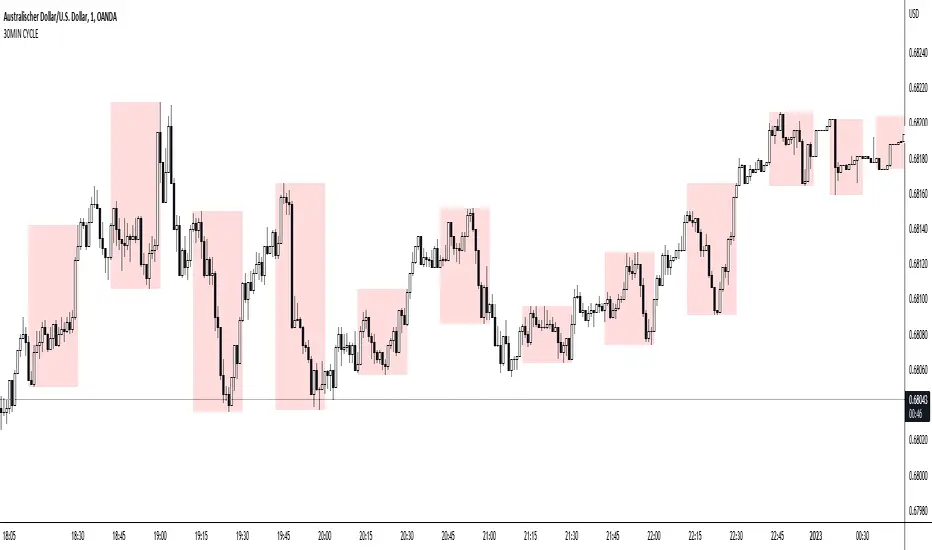
30MIN CYCLE█ HOW DOES IT WORK?
The known 90 min cycle is used as one killzone. But actually all 18 min are relevant to search for a trade. All 18 min when a new box starts only then is the placement of an order valid. If the entry candle isn't in a box then it will probably fail. The boxes should only be used in the M1 or M5 timeframe. The best hitrate is in the M1 timeframe. Included are the last 48 "Mini-Killzones" für intraday trading and backtesting. These "Mini-Killzones" can be used with the "Liquidity Inducement Strategy".
█ WHAT MAKES IT UNIQUE?
This is the first indicator on tradingview that shows all mini-killzones for trading and backtesting a whole tradingday. The well-known killzones of ICT are from 08:00-11:00 and 14:00 - 17:00 (UTC+1) but with this indicator there is finally a refinement of the ICT Smart Money Concept killzones.
█ HOW TO USE IT?
For a proper use of this indicator we suggest to know already at least SMC or better Liquidity Indcuement Trading. This indicator is a further confluence before placing an order. After you made your setup you will have these mini-killzones as a confluence. We don't suggest to open a trade only according to this indicator.
█ ADDITIONAL INFO
This indicator is free to use for all tradingview users.
█ DISCLAIMER
This is not financial advice.
DRM StrategyOne of the ways I go when I develop strategies is by reducing the number of parameters and removing fixed parameters and levels.
In this strategy, I'm trying to create an RSI indicator with a dynamic length.
Length is computed based on the correlation between Price and its momentum.
You can set min and max values for the RSI, and if the correlation is close to 1, we'll be at a min RSI value. When it's -1, we'll be at the max level.
I got this idea from Sofien Kaabar's book.
The strategy is super simple, and there might be much room for improvement.
Performance on the deep backtesting is not excellent, so I think the strategy needs some filters for regimes, etc.
Thanks to @MUQWISHI for helping me code it.
Disclaimer
Please remember that past performance may not indicate future results.
Due to various factors, including changing market conditions, the strategy may no longer perform as well as in historical backtesting.
This post and the script don’t provide any financial advice.

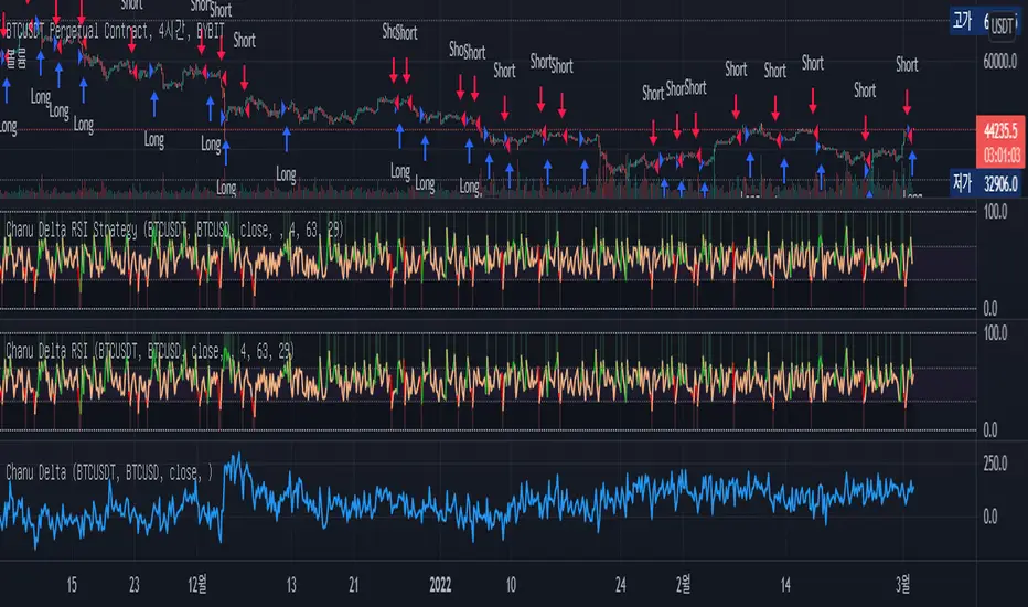
Chanu Delta RSI StrategyThis strategy is built on the Chanu Delta RSI , which indicates the strength of the Bitcoin market. The problem with the previous Chanu Delta Strategy was that it was simply based on the price difference between the two Bitcoin markets, so there was no universality. However, this new Chanu Delta RSI strategy solves the problem by introducing an RSI that compares the price difference trend.
When the Chanu Delta RSI hits “Bull Level” and “Bear Level” and closes the candle, long and short signals are triggered respectively. The example shown on the screen is a default setting optimized for a 4-hour candlestick strategy based on the Bybit BTCUSDT futures market. You can use it by adjusting the setting value and modifying it to suit you.
This strategy is selectable from both reference and large amplitude BTCUSD markets in order to enable fine backtesting. I recommend using BYBIT:BTCUSDT for the reference market and COINBASE:BTCUSD for the large amplitude market.
(Note) Using the "Chanu Delta RSI" to know the current indicator value in real time, it is convenient to predict the signal of the strategy.
(Note) Because the Chanu Delta RSI represents the price difference based on the Bybit BTCUSDT futures market, backtesting is possible from March 2020.
_____________________________________________________________
이 전략은 비트코인 시장의 강점을 나타내는 Chanu Delta RSI를 기반으로 합니다. 기존 Chanu Delta 전략의 문제점은 단순히 두 비트코인 시장의 가격차를 기준으로 하여 보편성이 없었다는 점이다. 하지만 이번 새로운 Chanu Delta RSI 전략은 가격차이 추세를 비교하는 RSI를 도입해 문제를 해결했습니다.
Chanu Delta RSI가 "Bull Level"과 "Bear Level"에 도달하고 봉마감하면 롱, 숏 신호가 각각 트리거됩니다. 화면에 보이는 예시는 Bybit BTCUSDT 선물 시장을 기반으로 한 4시간 캔들스틱 전략에 최적화된 기본 설정입니다. 설정값을 조정하여 자신에게 맞게 수정하여 사용하시면 됩니다.
이 전략은 정밀한 백테스팅을 가능하게 하기 위해 참조 및 큰 진폭 BTCUSD 시장에서 모두 선택할 수 있습니다. 참조 시장에는 BYBIT:BTCUSDT를 사용하고 큰 진폭 시장에는 COINBASE:BTCUSD를 사용하는 것이 좋습니다.
(주) "Chanu Delta RSI"를 이용하여 현재 지표 값을 실시간으로 알 수 있어 전략의 시그널을 예측하는데 편리합니다.
(주) Chanu Delta RSI는 바이비트 BTCUSDT 선물시장을 기준으로 가격차이를 나타내므로 2020년 3월부터 백테스팅이 가능합니다.
Breakout Trend Trading Strategy - V1Strategy in nutshell:
This strategy is made to be used in daily time-frames. Works better on trending instruments where volume is available. Hence, this is more suitable for trending shares rather than currencies, commodities and indexes where volume data is either not present or not reliable.
Breakout signifies the continuation of trend. Hence, trade in the direction of breakouts. Breakouts are calculated based on high volume and price movement in a day. This will be combined with few other conditions to generate buy and sell signals along with stop and compound targets. Supertrend is used for trend bias. Our buy and sell targets do not directly depend on the bias. But, entry criteria in opposite trend is made much difficult than that of trend direction. Further explanation of method and input parameters are explained below.
Backtesting parameters :
Capital and position sizing : Capital and position sizing parameters are set to test investing 2000 wholly on certain stock without compounding.
Initial Capital : 2000
Order Size : 100% of equity
Pyramiding : 1
ExitOnSignal : If unchecked exit is triggered solely on trailing stop
Trade Direction : Long, Short or All. Short condition is riskier than long conditions and often results in losses as per my observation. On most of the stocks trending up, strategy will not generate any short signals. This is achieved by comparing yearly high lows to previous two years to decide whether to allow short or long entries.
allowImmediateCompound : Applicable only if compounding/pyramiding is enabled in trade. If checked allows to place compounding orders immediately. If unchecked, it waits for stopline to cross order price before placing next compound.
Display Mode :
Targets : Whenever breakout happens, show marker for upTarget and downTarget
TargetChannel : Show up target and downtarget as a channel
Target With Stop : Along with targets, show also stop levels for breakouts
Up Channel : Channel created from UpTarget and respective stops
Down Channel : Channel created from DownTarget and respective stops
ShowTrailingStop : Shows trailing stop and compound lines when there is a trading position.
ShowTargetLevels : Shows Buy Sell target levels along with stop and compound lines. Trades are done as market orders. Hence, target levels are displayed after strategy makes the trade. Since only one order allowed per side without compounding, target, stop and compound levels are shown sometimes even without trade being made. These can be considered as entry levels if there is no existing position.
ShowPreviousLevels : Shows previous buy/sell target levels. When enabled, layout can look messy.
StopMultiplyer: To Set trailing stop loss.
BacktestYears: Number of years to include in backtest
So far my test cases are:
Positive : AAPL, AMZN, TSLA, RUN, VRT, ASX:APT
Negative Test Cases: WPL, WHC, NHC, WOW, COL, NAB (All ASX stocks)
Special test case: WDI
Negative test cases still show losses in backtesting. I have attempted including many conditions to eliminate or reduce the loss. But, further efforts has resulted in reduction in profits in positive cases as well. Still experimenting. Will update whenever I find improvements. Comments and suggestions welcome :)

Average True Range BandsThis is a simple script to assist you in manual backtesting! Perfect for the NNFX crowd or anyone that enjoys manual backtesting.
Usage
1. Slap this bad boy on your chart.
2. Adjust period and multiplier (defaults are 14 period and 1.5x).
3. Put on the indicator/system you are testing.
4. Enter bar replay mode.
5. Drag your long/short position take profit and stop loss to the upper and lower bands.
(long/short positions are available on the left-hand toolbar)
6. Profit!
If you enjoy/use this script, drop me a follow and please note me in your code!
I'm *almost* always available for collabs and questions.

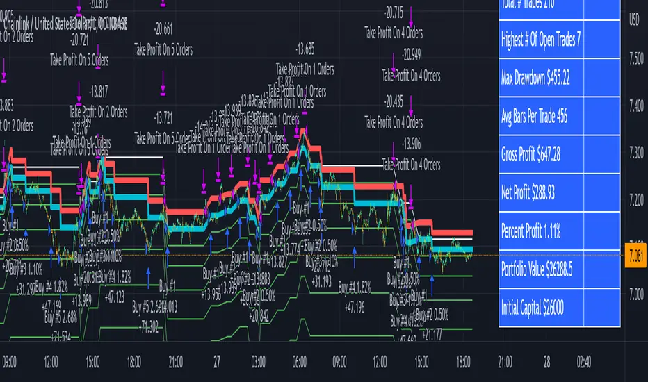
3Commas Bot DCA Backtester & Signals FREEThis is a DCA Strategy backtester + signals, built to emulate the 3Commas DCA bots. It uses your choice of 4 different buy signals, 2 of which can be adjusted in the settings. Everything is customizable so you can backtest specific settings with different buy signals and find the best performing strategy for your risk tolerance and capital. It can be used to backtest strategies on stocks as well, but just make sure your base order is larger than the share price for the entire backtesting range or it will not calculate properly.
You can use this template to code your own buy signals and then backtest them as a DCA strategy if you know some basic pine script.
The indicator shows all of your backtesting orders on the chart. The red line is your take profit level, the blue line is your average price level, the white line is your first order and the green lines are your average down orders. If you enable a stop loss in the settings your stop loss will be shown as an orange line once all of your average down orders have been hit, it will not be set until price has dipped below your covered trading range.
These levels update when things change during backtesting so you can visualize your strategy and how it would perform as well as see if your percentage deviation is large enough to cover dips. When backtesting trades are taken, the chart will show where they were taken(in backtesting) along with info on those trades such as the number each order is, the size of that order and the percentage deviation that order is from the initial buy.
SENDING SIGNALS TO 3COMMAS
Tradingview cannot sync this backtester to 3Commas and with the way alerts are setup for strategies on Tradingview, the best option for you to give signals to your bot would be to use this backtester to figure out what trigger you want to use and then setup that indicator separately to send alerts to your bot. All of the indicators used for signals in this backtester are available for free and can be configured to match this backtester and send alerts to 3Commas for you. Just make sure you set your alerts to once per bar close and don’t use less than a 15 second timeframe because then you could trigger the Tradingview threshold for alerts and get your alerts shut off.
You can also use this backtester with your own buy triggers if you know a little pine script. Just make copy of the script and code in your own buy signals and see how it backtests.
INFO PANEL FOR ANALYZING YOUR STRATEGY
The right hand side of the screen will show an info panel that shows a lot of different information so you can quickly see your bot settings and how it performed right on the screen.
In the top right corner you will see in purple your bot settings. These include your stoploss % if turned on, take profit %, average down order %, average down order % multiplier, volume multiplier, max number of orders allowed and size of your base order.
The top section of the first column “Current Trade” shows these stats: the open trade’s average price, the open trade’s take profit price, the open trade’s PNL, how far price is from your open tarde’s take profit level in percentage, your open position size and number of open orders.
The bottom section of the first column “Overall Performance” shows these stats: total number of trades taken during backtesting range, the largest amount of trades that were open at one time during backtesting, the max drawdown, the average number of bars per trade, gross profit, net profit, percent profit from your initial capital, current portfolio value and your initial capital.
CUSTOMIZABLE OPTIONS TO FIND THE PERFECT STRATEGY
Stoploss On/Off
This will turn your stoploss on or off. By default it is set to off and will not affect anything unless turned on.
Stoploss Percentage
This is the percentage below your final average down order price that will be set as a stoploss to keep your account from going too far in the red on big dips.
Take Profit Percentage - This is the percentage of profit you want the trade to hit before taking profit on your entire DCA trade. This level updates everytime you average down.
Average Down Percentage - This is the percentage that price has to drop from your initial order to initiate your first safety order. If the Average Down Percent Multiplier is set to 1 then this percentage will be the same for every average down order.
Average Down Percentage Multiplier - This multiplies your Average Down Percentage so each safety order needs a larger percentage deviation than the previous one. This keeps your buys closer together at the beginning and further apart when you hit more orders so you can extend your trading range but still be aggressive when price is going sideways.
Volume Multiplier Per New Order - This multiplies the size of each trade based on your base order. If you set it to a 2x multiplier then each average down order will be 2 times the size of the last one. So for example, a $100 base order with a 2x multiplier would have these values for the first 3 average down orders: 200, 400, 800.
Size Of Base Order - This is the size of your first position entry and will be used as a starting point for the volume multiplier. If your base order is $100 then it will buy $100 worth of whatever crypto you are backtesting this on. If you are looking at stock charts, you need to make sure your base order is higher than the share price across the entire backtesting range or it will not perform correctly.
Max Number Of Orders - This is the maximum number of orders the bot can take, including your base order. Adjust this to suit the amount of capital you are willing to allocate to your bot based on how much money it will require to run according to your bot settings.
TIPS ON HOW TO USE FOR BEST RESULTS
If you don’t have a lot of capital to work with, then use longer timeframes with a reasonable take profit percentage so that you don’t need a lot of average down orders. You can also try keeping the volume multiplier close to 1.
You can use the 3Commas dca bot settings page to see how much capital you will need for your strategy if you match it to the settings you have on this indicator. You can also check to see how much of a percentage deviation your bot is covering to make sure you have a reasonable range to trade in and orders to cover big dips. You can also check your coverage by seeing how far down the chart the green lines cover, which are your average down orders.
Make sure the initial capital in the properties tab of the settings has enough to cover all of your orders otherwise you will get unrealistic backtesting results. Also, make sure you leave the order size in the properties tab on contracts so it calculates your trades correctly. The only settings you need to touch in the properties tab is the initial capital. Unless you are trading somewhere that has lower commission fees, then you can change that to match, but leave all the other settings as is for it to function properly.
Increasing the volume multiplier will make your average price and take profit target follow the price action a lot closer as price falls, but it can also lead to having very large orders very quickly once you get into the 1.5-3x multiple range. Try using a high volume multiplier with less safety orders and you will get better results, however you need to have money on the sidelines to add on major dips to keep your bot turning a profit. Be very careful with this as greed and impatience will hurt your overall performance. This bot is meant to make money with lots of small wins so don’t get greedy and make sure you have enough money to cover large dips. If you are being aggressive with your bot, then I recommend only using 25% or less of your portfolio to trade aggressively and then use the smart trade feature on 3commas to add chunks of funds to your trades when price dips below your last safety order. Or if you want it to run without any supervision, then use lower volume multipliers and have lots of safety orders that can cover entire bear markets and still keep buying lower.
It’s a good idea to have some capital on the sidelines that you can add in when price dips quickly. This will help lower your average price and allow your bot to get out in profit quicker. 3Commas bot has a smart trade feature that will allow you to track your average price when adding extra funds and it will automatically update your other orders which is very convenient. Look at the longer timeframes when price dips and only add chunks at major areas where price is very likely to bounce. Or you can be aggressive when trading and add to your position when price dips and is at a likely bounce zone to maximize profits.
Only trade coins that have a good amount of liquidity as the larger your orders get, the harder it will be to sell if there isn’t much liquidity. Also, beware of how large your first order is as it will usually be a market order and can move the market if there is not much liquidity.
Since this bot takes a lot of trades and performs best when taking small profits consistently, you will need to factor in exchange fees. The bot is set to .5% commission(you can change this) on the buy and sell orders as most exchanges charge that amount. Some exchanges offer no fee trading on certain coins so be sure to look around for those so you can keep the commissions and maximize profits.
I strongly encourage you to try out a lot of different setting combinations across multiple different coins and do it across a few months to see how it would have performed under various market conditions. This will help you get a better idea of how much of a percentage deviation you’ll need to be able to cover to keep your bot running and making constant profits. You can also use the deep backtesting feature of the strategy panel to see how it would have done, but just beware that the info panel of the indicator will not reflect deep backtesting results, only the normal backtesting range.
MARKETS
This backtester can be used on any market including crypto, stocks, forex & futures. You just need to make sure your base order is larger than the share price when using this on things besides crypto.
TIMEFRAMES
This backtester can be used on all timeframes.
HolidayLibrary "Holiday"
- Full Control over Holidays and Daylight Savings Time (DLS)
The Holiday Library is an essential tool for traders and analysts who engage in backtesting and live trading . This comprehensive library enables the incorporation of crucial calendar elements - specifically Daylight Savings Time (DLS) adjustments and public holidays - into trading strategies and backtesting environments.
Key Features:
- DLS Adjustments: The library takes into account the shifts in time due to Daylight Savings. This feature is particularly vital for backtesting strategies, as DLS can impact trading hours, which in turn affects the volatility and liquidity in the market. Accurate DLS adjustments ensure that backtesting scenarios are as close to real-life conditions as possible.
- Comprehensive Holiday Metadata: The library includes a rich set of holiday metadata, allowing for the detailed scheduling of trading activities around public holidays. This feature is crucial for avoiding skewed results in backtesting, where holiday trading sessions might differ significantly in terms of volume and price movement.
- Customizable Holiday Schedules: Users can add or remove specific holidays, tailoring the library to fit various regional market schedules or specific trading requirements.
- Visualization Aids: The library supports on-chart labels, making it visually intuitive to identify holidays and DLS shifts directly on trading charts.
Use Cases:
1. Strategy Development: When developing trading strategies, it’s important to account for non-trading days and altered trading hours due to holidays and DLS. This library enables a realistic and accurate representation of these factors.
2. Risk Management: Trading around holidays can be riskier due to thinner liquidity and greater volatility. By integrating holiday data, traders can better manage their risk exposure.
3. Backtesting Accuracy: For backtesting to be effective, it must simulate the actual market conditions as closely as possible. Incorporating holidays and DLS adjustments contributes to more reliable and realistic backtesting results.
4. Global Trading: For traders active in multiple global markets, this library provides an easy way to handle different holiday schedules and DLS shifts across regions.
The Holiday Library is a versatile tool that enhances the precision and realism of trading simulations and strategy development . Its integration into the trading workflow is straightforward and beneficial for both novice and experienced traders.
EasterAlgo(_year)
Calculates the date of Easter Sunday for a given year using the Anonymous Gregorian algorithm.
`Gauss Algorithm for Easter Sunday` was developed by the mathematician Carl Friedrich Gauss
This algorithm is based on the cycles of the moon and the fact that Easter always falls on the first Sunday after the first ecclesiastical full moon that occurs on or after March 21.
While it's not considered to be 100% accurate due to rare exceptions, it does give the correct date in most cases.
It's important to note that Gauss's formula has been found to be inaccurate for some 21st-century years in the Gregorian calendar. Specifically, the next suggested failure years are 2038, 2051.
This function can be used for Good Friday (Friday before Easter), Easter Sunday, and Easter Monday (following Monday).
en.wikipedia.org
Parameters:
_year (int) : `int` - The year for which to calculate the date of Easter Sunday. This should be a four-digit year (YYYY).
Returns: tuple - The month (1-12) and day (1-31) of Easter Sunday for the given year.
easterInit()
Inits the date of Easter Sunday and Good Friday for a given year.
Returns: tuple - The month (1-12) and day (1-31) of Easter Sunday and Good Friday for the given year.
isLeapYear(_year)
Determine if a year is a leap year.
Parameters:
_year (int) : `int` - 4 digit year to check => YYYY
Returns: `bool` - true if input year is a leap year
method timezoneHelper(utc)
Helper function to convert UTC time.
Namespace types: series int, simple int, input int, const int
Parameters:
utc (int) : `int` - UTC time shift in hours.
Returns: `string`- UTC time string with shift applied.
weekofmonth()
Function to find the week of the month of a given Unix Time.
Returns: number - The week of the month of the specified UTC time.
dayLightSavingsAdjustedUTC(utc, adjustForDLS)
dayLightSavingsAdjustedUTC
Parameters:
utc (int) : `int` - The normal UTC timestamp to be used for reference.
adjustForDLS (bool) : `bool` - Flag indicating whether to adjust for daylight savings time (DLS).
Returns: `int` - The adjusted UTC timestamp for the given normal UTC timestamp.
getDayOfYear(monthOfYear, dayOfMonth, weekOfMonth, dayOfWeek, lastOccurrenceInMonth, holiday)
Function gets the day of the year of a given holiday (1-366)
Parameters:
monthOfYear (int)
dayOfMonth (int)
weekOfMonth (int)
dayOfWeek (int)
lastOccurrenceInMonth (bool)
holiday (string)
Returns: `int` - The day of the year of the holiday 1-366.
method buildMap(holidayMap, holiday, monthOfYear, weekOfMonth, dayOfWeek, dayOfMonth, lastOccurrenceInMonth, closingTime)
Function to build the `holidaysMap`.
Namespace types: map
Parameters:
holidayMap (map) : `map` - The map of holidays.
holiday (string) : `string` - The name of the holiday.
monthOfYear (int) : `int` - The month of the year of the holiday.
weekOfMonth (int) : `int` - The week of the month of the holiday.
dayOfWeek (int) : `int` - The day of the week of the holiday.
dayOfMonth (int) : `int` - The day of the month of the holiday.
lastOccurrenceInMonth (bool) : `bool` - Flag indicating whether the holiday is the last occurrence of the day in the month.
closingTime (int) : `int` - The closing time of the holiday.
Returns: `map` - The updated map of holidays
holidayInit(addHolidaysArray, removeHolidaysArray, defaultHolidays)
Initializes a HolidayStorage object with predefined US holidays.
Parameters:
addHolidaysArray (array) : `array` - The array of additional holidays to be added.
removeHolidaysArray (array) : `array` - The array of holidays to be removed.
defaultHolidays (bool) : `bool` - Flag indicating whether to include the default holidays.
Returns: `map` - The map of holidays.
Holidays(utc, addHolidaysArray, removeHolidaysArray, adjustForDLS, displayLabel, defaultHolidays)
Main function to build the holidays object, this is the only function from this library that should be needed. \
all functionality should be available through this function. \
With the exception of initializing a `HolidayMetaData` object to add a holiday or early close. \
\
**Default Holidays:** \
`DLS begin`, `DLS end`, `New Year's Day`, `MLK Jr. Day`, \
`Washington Day`, `Memorial Day`, `Independence Day`, `Labor Day`, \
`Columbus Day`, `Veterans Day`, `Thanksgiving Day`, `Christmas Day` \
\
**Example**
```
HolidayMetaData valentinesDay = HolidayMetaData.new(holiday="Valentine's Day", monthOfYear=2, dayOfMonth=14)
HolidayMetaData stPatricksDay = HolidayMetaData.new(holiday="St. Patrick's Day", monthOfYear=3, dayOfMonth=17)
HolidayMetaData addHolidaysArray = array.from(valentinesDay, stPatricksDay)
string removeHolidaysArray = array.from("DLS begin", "DLS end")
܂Holidays = Holidays(
܂ utc=-6,
܂ addHolidaysArray=addHolidaysArray,
܂ removeHolidaysArray=removeHolidaysArray,
܂ adjustForDLS=true,
܂ displayLabel=true,
܂ defaultHolidays=true,
܂ )
plot(Holidays.newHoliday ? open : na, title="newHoliday", color=color.red, linewidth=4, style=plot.style_circles)
```
Parameters:
utc (int) : `int` - The UTC time shift in hours
addHolidaysArray (array) : `array` - The array of additional holidays to be added
removeHolidaysArray (array) : `array` - The array of holidays to be removed
adjustForDLS (bool) : `bool` - Flag indicating whether to adjust for daylight savings time (DLS)
displayLabel (bool) : `bool` - Flag indicating whether to display a label on the chart
defaultHolidays (bool) : `bool` - Flag indicating whether to include the default holidays
Returns: `HolidayObject` - The holidays object | Holidays = (holidaysMap: map, newHoliday: bool, holiday: string, dayString: string)
HolidayMetaData
HolidayMetaData
Fields:
holiday (series string) : `string` - The name of the holiday.
dayOfYear (series int) : `int` - The day of the year of the holiday.
monthOfYear (series int) : `int` - The month of the year of the holiday.
dayOfMonth (series int) : `int` - The day of the month of the holiday.
weekOfMonth (series int) : `int` - The week of the month of the holiday.
dayOfWeek (series int) : `int` - The day of the week of the holiday.
lastOccurrenceInMonth (series bool)
closingTime (series int) : `int` - The closing time of the holiday.
utc (series int) : `int` - The UTC time shift in hours.
HolidayObject
HolidayObject
Fields:
holidaysMap (map) : `map` - The map of holidays.
newHoliday (series bool) : `bool` - Flag indicating whether today is a new holiday.
activeHoliday (series bool) : `bool` - Flag indicating whether today is an active holiday.
holiday (series string) : `string` - The name of the holiday.
dayString (series string) : `string` - The day of the week of the holiday.
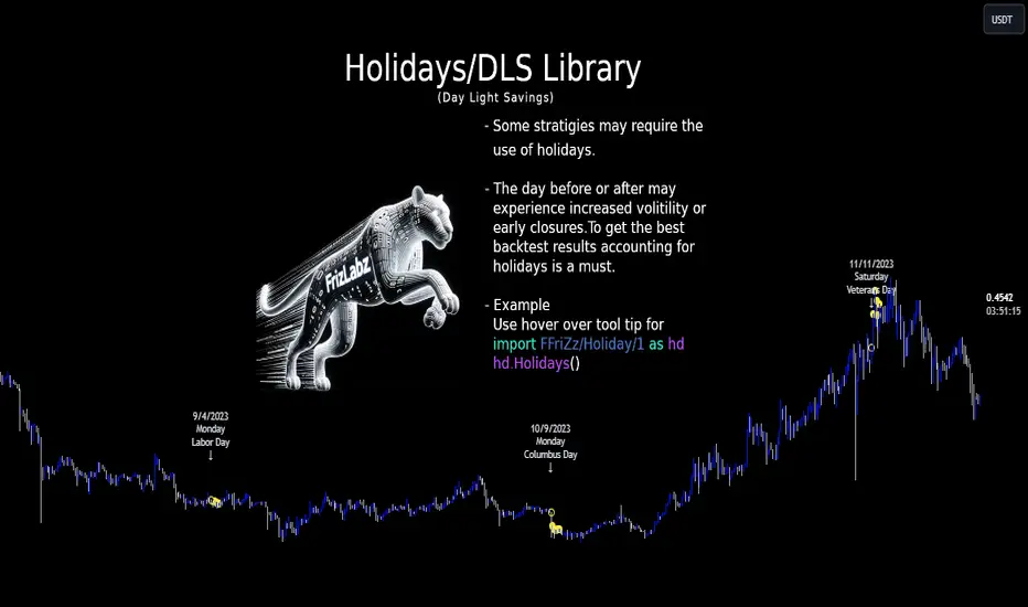
Supertrend Advance Pullback StrategyHandbook for the Supertrend Advance Strategy
1. Introduction
Purpose of the Handbook:
The main purpose of this handbook is to serve as a comprehensive guide for traders and investors who are looking to explore and harness the potential of the Supertrend Advance Strategy. In the rapidly changing financial market, having the right tools and strategies at one's disposal is crucial. Whether you're a beginner hoping to dive into the world of trading or a seasoned investor aiming to optimize and diversify your portfolio, this handbook offers the insights and methodologies you need. By the end of this guide, readers should have a clear understanding of how the Supertrend Advance Strategy works, its benefits, potential pitfalls, and practical application in various trading scenarios.
Overview of the Supertrend Advance Pullback Strategy:
At its core, the Supertrend Advance Strategy is an evolution of the popular Supertrend Indicator. Designed to generate buy and sell signals in trending markets, the Supertrend Indicator has been a favorite tool for many traders around the world. The Advance Strategy, however, builds upon this foundation by introducing enhanced mechanisms, filters, and methodologies to increase precision and reduce false signals.
1. Basic Concept:
The Supertrend Advance Strategy relies on a combination of price action and volatility to determine the potential trend direction. By assessing the average true range (ATR) in conjunction with specific price points, this strategy aims to highlight the potential starting and ending points of market trends.
2. Methodology:
Unlike the traditional Supertrend Indicator, which primarily focuses on closing prices and ATR, the Advance Strategy integrates other critical market variables, such as volume, momentum oscillators, and perhaps even fundamental data, to validate its signals. This multidimensional approach ensures that the generated signals are more reliable and are less prone to market noise.
3. Benefits:
One of the main benefits of the Supertrend Advance Strategy is its ability to filter out false breakouts and minor price fluctuations, which can often lead to premature exits or entries in the market. By waiting for a confluence of factors to align, traders using this advanced strategy can increase their chances of entering or exiting trades at optimal points.
4. Practical Applications:
The Supertrend Advance Strategy can be applied across various timeframes, from intraday trading to swing trading and even long-term investment scenarios. Furthermore, its flexible nature allows it to be tailored to different asset classes, be it stocks, commodities, forex, or cryptocurrencies.
In the subsequent sections of this handbook, we will delve deeper into the intricacies of this strategy, offering step-by-step guidelines on its application, case studies, and tips for maximizing its efficacy in the volatile world of trading.
As you journey through this handbook, we encourage you to approach the Supertrend Advance Strategy with an open mind, testing and tweaking it as per your personal trading style and risk appetite. The ultimate goal is not just to provide you with a new tool but to empower you with a holistic strategy that can enhance your trading endeavors.
2. Getting Started
Navigating the financial markets can be a daunting task without the right tools. This section is dedicated to helping you set up the Supertrend Advance Strategy on one of the most popular charting platforms, TradingView. By following the steps below, you'll be able to integrate this strategy into your charts and start leveraging its insights in no time.
Setting up on TradingView:
TradingView is a web-based platform that offers a wide range of charting tools, social networking, and market data. Before you can apply the Supertrend Advance Strategy, you'll first need a TradingView account. If you haven't set one up yet, here's how:
1. Account Creation:
• Visit TradingView's official website.
• Click on the "Join for free" or "Sign up" button.
• Follow the registration process, providing the necessary details and setting up your login credentials.
2. Navigating the Dashboard:
• Once logged in, you'll be taken to your dashboard. Here, you'll see a variety of tools, including watchlists, alerts, and the main charting window.
• To begin charting, type in the name or ticker of the asset you're interested in the search bar at the top.
3. Configuring Chart Settings:
• Before integrating the Supertrend Advance Strategy, familiarize yourself with the chart settings. This can be accessed by clicking the 'gear' icon on the top right of the chart window.
• Adjust the chart type, time intervals, and other display settings to your preference.
Integrating the Strategy into a Chart:
Now that you're set up on TradingView, it's time to integrate the Supertrend Advance Strategy.
1. Accessing the Pine Script Editor:
• Located at the top-center of your screen, you'll find the "Pine Editor" tab. Click on it.
• This is where custom strategies and indicators are scripted or imported.
2. Loading the Supertrend Advance Strategy Script:
• Depending on whether you have the script or need to find it, there are two paths:
• If you have the script: Copy the Supertrend Advance Strategy script, and then paste it into the Pine Editor.
• If searching for the script: Click on the “Indicators” icon (looks like a flame) at the top of your screen, and then type “Supertrend Advance Strategy” in the search bar. If available, it will show up in the list. Simply click to add it to your chart.
3. Applying the Strategy:
• After pasting or selecting the Supertrend Advance Strategy in the Pine Editor, click on the “Add to Chart” button located at the top of the editor. This will overlay the strategy onto your main chart window.
4. Configuring Strategy Settings:
• Once the strategy is on your chart, you'll notice a small settings ('gear') icon next to its name in the top-left of the chart window. Click on this to access settings.
• Here, you can adjust various parameters of the Supertrend Advance Strategy to better fit your trading style or the specific asset you're analyzing.
5. Interpreting Signals:
• With the strategy applied, you'll now see buy/sell signals represented on your chart. Take time to familiarize yourself with how these look and behave over various timeframes and market conditions.
3. Strategy Overview
What is the Supertrend Advance Strategy?
The Supertrend Advance Strategy is a refined version of the classic Supertrend Indicator, which was developed to aid traders in spotting market trends. The strategy utilizes a combination of data points, including average true range (ATR) and price momentum, to generate buy and sell signals.
In essence, the Supertrend Advance Strategy can be visualized as a line that moves with the price. When the price is above the Supertrend line, it indicates an uptrend and suggests a potential buy position. Conversely, when the price is below the Supertrend line, it hints at a downtrend, suggesting a potential selling point.
Strategy Goals and Objectives:
1. Trend Identification: At the core of the Supertrend Advance Strategy is the goal to efficiently and consistently identify prevailing market trends. By recognizing these trends, traders can position themselves to capitalize on price movements in their favor.
2. Reducing Noise: Financial markets are often inundated with 'noise' - short-term price fluctuations that can mislead traders. The Supertrend Advance Strategy aims to filter out this noise, allowing for clearer decision-making.
3. Enhancing Risk Management: With clear buy and sell signals, traders can set more precise stop-loss and take-profit points. This leads to better risk management and potentially improved profitability.
4. Versatility: While primarily used for trend identification, the strategy can be integrated with other technical tools and indicators to create a comprehensive trading system.
Type of Assets/Markets to Apply the Strategy:
1. Equities: The Supertrend Advance Strategy is highly popular among stock traders. Its ability to capture long-term trends makes it particularly useful for those trading individual stocks or equity indices.
2. Forex: Given the 24-hour nature of the Forex market and its propensity for trends, the Supertrend Advance Strategy is a valuable tool for currency traders.
3. Commodities: Whether it's gold, oil, or agricultural products, commodities often move in extended trends. The strategy can help in identifying and capitalizing on these movements.
4. Cryptocurrencies: The volatile nature of cryptocurrencies means they can have pronounced trends. The Supertrend Advance Strategy can aid crypto traders in navigating these often tumultuous waters.
5. Futures & Options: Traders and investors in derivative markets can utilize the strategy to make more informed decisions about contract entries and exits.
It's important to note that while the Supertrend Advance Strategy can be applied across various assets and markets, its effectiveness might vary based on market conditions, timeframe, and the specific characteristics of the asset in question. As always, it's recommended to use the strategy in conjunction with other analytical tools and to backtest its effectiveness in specific scenarios before committing to trades.
4. Input Settings
Understanding and correctly configuring input settings is crucial for optimizing the Supertrend Advance Strategy for any specific market or asset. These settings, when tweaked correctly, can drastically impact the strategy's performance.
Grouping Inputs:
Before diving into individual input settings, it's important to group similar inputs. Grouping can simplify the user interface, making it easier to adjust settings related to a specific function or indicator.
Strategy Choice:
This input allows traders to select from various strategies that incorporate the Supertrend indicator. Options might include "Supertrend with RSI," "Supertrend with MACD," etc. By choosing a strategy, the associated input settings for that strategy become available.
Supertrend Settings:
1. Multiplier: Typically, a default value of 3 is used. This multiplier is used in the ATR calculation. Increasing it makes the Supertrend line further from prices, while decreasing it brings the line closer.
2. Period: The number of bars used in the ATR calculation. A common default is 7.
EMA Settings (Exponential Moving Average):
1. Period: Defines the number of previous bars used to calculate the EMA. Common periods are 9, 21, 50, and 200.
2. Source: Allows traders to choose which price (Open, Close, High, Low) to use in the EMA calculation.
RSI Settings (Relative Strength Index):
1. Length: Determines how many periods are used for RSI calculation. The standard setting is 14.
2. Overbought Level: The threshold at which the asset is considered overbought, typically set at 70.
3. Oversold Level: The threshold at which the asset is considered oversold, often at 30.
MACD Settings (Moving Average Convergence Divergence):
1. Short Period: The shorter EMA, usually set to 12.
2. Long Period: The longer EMA, commonly set to 26.
3. Signal Period: Defines the EMA of the MACD line, typically set at 9.
CCI Settings (Commodity Channel Index):
1. Period: The number of bars used in the CCI calculation, often set to 20.
2. Overbought Level: Typically set at +100, denoting overbought conditions.
3. Oversold Level: Usually set at -100, indicating oversold conditions.
SL/TP Settings (Stop Loss/Take Profit):
1. SL Multiplier: Defines the multiplier for the average true range (ATR) to set the stop loss.
2. TP Multiplier: Defines the multiplier for the average true range (ATR) to set the take profit.
Filtering Conditions:
This section allows traders to set conditions to filter out certain signals. For example, one might only want to take buy signals when the RSI is below 30, ensuring they buy during oversold conditions.
Trade Direction and Backtest Period:
1. Trade Direction: Allows traders to specify whether they want to take long trades, short trades, or both.
2. Backtest Period: Specifies the time range for backtesting the strategy. Traders can choose from options like 'Last 6 months,' 'Last 1 year,' etc.
It's essential to remember that while default settings are provided for many of these tools, optimal settings can vary based on the market, timeframe, and trading style. Always backtest new settings on historical data to gauge their potential efficacy.
5. Understanding Strategy Conditions
Developing an understanding of the conditions set within a trading strategy is essential for traders to maximize its potential. Here, we delve deep into the logic behind these conditions, using the Supertrend Advance Strategy as our focal point.
Basic Logic Behind Conditions:
Every strategy is built around a set of conditions that provide buy or sell signals. The conditions are based on mathematical or statistical methods and are rooted in the study of historical price data. The fundamental idea is to recognize patterns or behaviors that have been profitable in the past and might be profitable in the future.
Buy and Sell Conditions:
1. Buy Conditions: Usually formulated around bullish signals or indicators suggesting upward price momentum.
2. Sell Conditions: Centered on bearish signals or indicators indicating downward price momentum.
Simple Strategy:
The simple strategy could involve using just the Supertrend indicator. Here:
• Buy: When price closes above the Supertrend line.
• Sell: When price closes below the Supertrend line.
Pullback Strategy:
This strategy capitalizes on price retracements:
• Buy: When the price retraces to the Supertrend line after a bullish signal and is supported by another bullish indicator.
• Sell: When the price retraces to the Supertrend line after a bearish signal and is confirmed by another bearish indicator.
Indicators Used:
EMA (Exponential Moving Average):
• Logic: EMA gives more weight to recent prices, making it more responsive to current price movements. A shorter-period EMA crossing above a longer-period EMA can be a bullish sign, while the opposite is bearish.
RSI (Relative Strength Index):
• Logic: RSI measures the magnitude of recent price changes to analyze overbought or oversold conditions. Values above 70 are typically considered overbought, and values below 30 are considered oversold.
MACD (Moving Average Convergence Divergence):
• Logic: MACD assesses the relationship between two EMAs of a security’s price. The MACD line crossing above the signal line can be a bullish signal, while crossing below can be bearish.
CCI (Commodity Channel Index):
• Logic: CCI compares a security's average price change with its average price variation. A CCI value above +100 may mean the price is overbought, while below -100 might signify an oversold condition.
And others...
As the strategy expands or contracts, more indicators might be added or removed. The crucial point is to understand the core logic behind each, ensuring they align with the strategy's objectives.
Logic Behind Each Indicator:
1. EMA: Emphasizes recent price movements; provides dynamic support and resistance levels.
2. RSI: Indicates overbought and oversold conditions based on recent price changes.
3. MACD: Showcases momentum and direction of a trend by comparing two EMAs.
4. CCI: Measures the difference between a security's price change and its average price change.
Understanding strategy conditions is not just about knowing when to buy or sell but also about comprehending the underlying market dynamics that those conditions represent. As you familiarize yourself with each condition and indicator, you'll be better prepared to adapt and evolve with the ever-changing financial markets.
6. Trade Execution and Management
Trade execution and management are crucial aspects of any trading strategy. Efficient execution can significantly impact profitability, while effective management can preserve capital during adverse market conditions. In this section, we'll explore the nuances of position entry, exit strategies, and various Stop Loss (SL) and Take Profit (TP) methodologies within the Supertrend Advance Strategy.
Position Entry:
Effective trade entry revolves around:
1. Timing: Enter at a point where the risk-reward ratio is favorable. This often corresponds to confirmatory signals from multiple indicators.
2. Volume Analysis: Ensure there's adequate volume to support the movement. Volume can validate the strength of a signal.
3. Confirmation: Use multiple indicators or chart patterns to confirm the entry point. For instance, a buy signal from the Supertrend indicator can be confirmed with a bullish MACD crossover.
Position Exit Strategies:
A successful exit strategy will lock in profits and minimize losses. Here are some strategies:
1. Fixed Time Exit: Exiting after a predetermined period.
2. Percentage-based Profit Target: Exiting after a certain percentage gain.
3. Indicator-based Exit: Exiting when an indicator gives an opposing signal.
Percentage-based SL/TP:
• Stop Loss (SL): Set a fixed percentage below the entry price to limit potential losses.
• Example: A 2% SL on an entry at $100 would trigger a sell at $98.
• Take Profit (TP): Set a fixed percentage above the entry price to lock in gains.
• Example: A 5% TP on an entry at $100 would trigger a sell at $105.
Supertrend-based SL/TP:
• Stop Loss (SL): Position the SL at the Supertrend line. If the price breaches this line, it could indicate a trend reversal.
• Take Profit (TP): One could set the TP at a point where the Supertrend line flattens or turns, indicating a possible slowdown in momentum.
Swing high/low-based SL/TP:
• Stop Loss (SL): For a long position, set the SL just below the recent swing low. For a short position, set it just above the recent swing high.
• Take Profit (TP): For a long position, set the TP near a recent swing high or resistance. For a short position, near a swing low or support.
And other methods...
1. Trailing Stop Loss: This dynamic SL adjusts with the price movement, locking in profits as the trade moves in your favor.
2. Multiple Take Profits: Divide the position into segments and set multiple TP levels, securing profits in stages.
3. Opposite Signal Exit: Exit when another reliable indicator gives an opposite signal.
Trade execution and management are as much an art as they are a science. They require a blend of analytical skill, discipline, and intuition. Regularly reviewing and refining your strategies, especially in light of changing market conditions, is crucial to maintaining consistent trading performance.
7. Visual Representations
Visual tools are essential for traders, as they simplify complex data into an easily interpretable format. Properly analyzing and understanding the plots on a chart can provide actionable insights and a more intuitive grasp of market conditions. In this section, we’ll delve into various visual representations used in the Supertrend Advance Strategy and their significance.
Understanding Plots on the Chart:
Charts are the primary visual aids for traders. The arrangement of data points, lines, and colors on them tell a story about the market's past, present, and potential future moves.
1. Data Points: These represent individual price actions over a specific timeframe. For instance, a daily chart will have data points showing the opening, closing, high, and low prices for each day.
2. Colors: Used to indicate the nature of price movement. Commonly, green is used for bullish (upward) moves and red for bearish (downward) moves.
Trend Lines:
Trend lines are straight lines drawn on a chart that connect a series of price points. Their significance:
1. Uptrend Line: Drawn along the lows, representing support. A break below might indicate a trend reversal.
2. Downtrend Line: Drawn along the highs, indicating resistance. A break above might suggest the start of a bullish trend.
Filled Areas:
These represent a range between two values on a chart, usually shaded or colored. For instance:
1. Bollinger Bands: The area between the upper and lower band is filled, giving a visual representation of volatility.
2. Volume Profile: Can show a filled area representing the amount of trading activity at different price levels.
Stop Loss and Take Profit Lines:
These are horizontal lines representing pre-determined exit points for trades.
1. Stop Loss Line: Indicates the level at which a trade will be automatically closed to limit losses. Positioned according to the trader's risk tolerance.
2. Take Profit Line: Denotes the target level to lock in profits. Set according to potential resistance (for long trades) or support (for short trades) or other technical factors.
Trailing Stop Lines:
A trailing stop is a dynamic form of stop loss that moves with the price. On a chart:
1. For Long Trades: Starts below the entry price and moves up with the price but remains static if the price falls, ensuring profits are locked in.
2. For Short Trades: Starts above the entry price and moves down with the price but remains static if the price rises.
Visual representations offer traders a clear, organized view of market dynamics. Familiarity with these tools ensures that traders can quickly and accurately interpret chart data, leading to more informed decision-making. Always ensure that the visual aids used resonate with your trading style and strategy for the best results.
8. Backtesting
Backtesting is a fundamental process in strategy development, enabling traders to evaluate the efficacy of their strategy using historical data. It provides a snapshot of how the strategy would have performed in past market conditions, offering insights into its potential strengths and vulnerabilities. In this section, we'll explore the intricacies of setting up and analyzing backtest results and the caveats one must be aware of.
Setting Up Backtest Period:
1. Duration: Determine the timeframe for the backtest. It should be long enough to capture various market conditions (bullish, bearish, sideways). For instance, if you're testing a daily strategy, consider a period of several years.
2. Data Quality: Ensure the data source is reliable, offering high-resolution and clean data. This is vital to get accurate backtest results.
3. Segmentation: Instead of a continuous period, sometimes it's helpful to backtest over distinct market phases, like a particular bear or bull market, to see how the strategy holds up in different environments.
Analyzing Backtest Results:
1. Performance Metrics: Examine metrics like the total return, annualized return, maximum drawdown, Sharpe ratio, and others to gauge the strategy's efficiency.
2. Win Rate: It's the ratio of winning trades to total trades. A high win rate doesn't always signify a good strategy; it should be evaluated in conjunction with other metrics.
3. Risk/Reward: Understand the average profit versus the average loss per trade. A strategy might have a low win rate but still be profitable if the average gain far exceeds the average loss.
4. Drawdown Analysis: Review the periods of losses the strategy could incur and how long it takes, on average, to recover.
9. Tips and Best Practices
Successful trading requires more than just knowing how a strategy works. It necessitates an understanding of when to apply it, how to adjust it to varying market conditions, and the wisdom to recognize and avoid common pitfalls. This section offers insightful tips and best practices to enhance the application of the Supertrend Advance Strategy.
When to Use the Strategy:
1. Market Conditions: Ideally, employ the Supertrend Advance Strategy during trending market conditions. This strategy thrives when there are clear upward or downward trends. It might be less effective during consolidative or sideways markets.
2. News Events: Be cautious around significant news events, as they can cause extreme volatility. It might be wise to avoid trading immediately before and after high-impact news.
3. Liquidity: Ensure you are trading in assets/markets with sufficient liquidity. High liquidity ensures that the price movements are more reflective of genuine market sentiment and not due to thin volume.
Adjusting Settings for Different Markets/Timeframes:
1. Markets: Each market (stocks, forex, commodities) has its own characteristics. It's essential to adjust the strategy's parameters to align with the market's volatility and liquidity.
2. Timeframes: Shorter timeframes (like 1-minute or 5-minute charts) tend to have more noise. You might need to adjust the settings to filter out false signals. Conversely, for longer timeframes (like daily or weekly charts), you might need to be more responsive to genuine trend changes.
3. Customization: Regularly review and tweak the strategy's settings. Periodic adjustments can ensure the strategy remains optimized for the current market conditions.
10. Frequently Asked Questions (FAQs)
Given the complexities and nuances of the Supertrend Advance Strategy, it's only natural for traders, both new and seasoned, to have questions. This section addresses some of the most commonly asked questions regarding the strategy.
1. What exactly is the Supertrend Advance Strategy?
The Supertrend Advance Strategy is an evolved version of the traditional Supertrend indicator. It's designed to provide clearer buy and sell signals by incorporating additional indicators like EMA, RSI, MACD, CCI, etc. The strategy aims to capitalize on market trends while minimizing false signals.
2. Can I use the Supertrend Advance Strategy for all asset types?
Yes, the strategy can be applied to various asset types like stocks, forex, commodities, and cryptocurrencies. However, it's crucial to adjust the settings accordingly to suit the specific characteristics and volatility of each asset type.
3. Is this strategy suitable for day trading?
Absolutely! The Supertrend Advance Strategy can be adjusted to suit various timeframes, making it versatile for both day trading and long-term trading. Remember to fine-tune the settings to align with the timeframe you're trading on.
4. How do I deal with false signals?
No strategy is immune to false signals. However, by combining the Supertrend with other indicators and adhering to strict risk management protocols, you can minimize the impact of false signals. Always use stop-loss orders and consider filtering trades with additional confirmation signals.
5. Do I need any prior trading experience to use this strategy?
While the Supertrend Advance Strategy is designed to be user-friendly, having a foundational understanding of trading and market analysis can greatly enhance your ability to employ the strategy effectively. If you're a beginner, consider pairing the strategy with further education and practice on demo accounts.
6. How often should I review and adjust the strategy settings?
There's no one-size-fits-all answer. Some traders adjust settings weekly, while others might do it monthly. The key is to remain responsive to changing market conditions. Regular backtesting can give insights into potential required adjustments.
7. Can the Supertrend Advance Strategy be automated?
Yes, many traders use algorithmic trading platforms to automate their strategies, including the Supertrend Advance Strategy. However, always monitor automated systems regularly to ensure they're operating as intended.
8. Are there any markets or conditions where the strategy shouldn't be used?
The strategy might generate more false signals in markets that are consolidative or range-bound. During significant news events or times of unexpected high volatility, it's advisable to tread with caution or stay out of the market.
9. How important is backtesting with this strategy?
Backtesting is crucial as it allows traders to understand how the strategy would have performed in the past, offering insights into potential profitability and areas of improvement. Always backtest any new setting or tweak before applying it to live trades.
10. What if the strategy isn't working for me?
No strategy guarantees consistent profits. If it's not working for you, consider reviewing your settings, seeking expert advice, or complementing the Supertrend Advance Strategy with other analysis methods. Remember, continuous learning and adaptation are the keys to trading success.
Other comments
Value of combining several indicators in this script and how they work together
Diversification of Signals: Just as diversifying an investment portfolio can reduce risk, using multiple indicators can offer varied perspectives on potential price movements. Each indicator can capture a different facet of the market, ensuring that traders are not overly reliant on a single data point.
Confirmation & Reduced False Signals: A common challenge with many indicators is the potential for false signals. By requiring confirmation from multiple indicators before acting, the chances of acting on a false signal can be significantly reduced.
Flexibility Across Market Conditions: Different indicators might perform better under different market conditions. For example, while moving averages might excel in trending markets, oscillators like RSI might be more useful during sideways or range-bound conditions. A mashup strategy can potentially adapt better to varying market scenarios.
Comprehensive Analysis: With multiple indicators, traders can gauge trend strength, momentum, volatility, and potential market reversals all at once, providing a holistic view of the market.
How do the different indicators in the Supertrend Advance Strategy work together?
Supertrend: This is primarily a trend-following indicator. It provides traders with buy and sell signals based on the volatility of the price. When combined with other indicators, it can filter out noise and give more weight to strong, confirmed trends.
EMA (Exponential Moving Average): EMA gives more weight to recent price data. It can be used to identify the direction and strength of a trend. When the price is above the EMA, it's generally considered bullish, and vice versa.
RSI (Relative Strength Index): An oscillator that measures the magnitude of recent price changes to evaluate overbought or oversold conditions. By cross-referencing with other indicators like EMA or MACD, traders can spot potential reversals or confirmations of a trend.
MACD (Moving Average Convergence Divergence): This indicator identifies changes in the strength, direction, momentum, and duration of a trend in a stock's price. When the MACD line crosses above the signal line, it can be a bullish sign, and when it crosses below, it can be bearish. Pairing MACD with Supertrend can provide dual confirmation of a trend.
CCI (Commodity Channel Index): Initially developed for commodities, CCI can indicate overbought or oversold conditions. It can be used in conjunction with other indicators to determine entry and exit points.
In essence, the synergy of these indicators provides a balanced, comprehensive approach to trading. Each indicator offers its unique lens into market conditions, and when they align, it can be a powerful indication of a trading opportunity. This combination not only reduces the potential drawbacks of each individual indicator but leverages their strengths, aiming for more consistent and informed trading decisions.
Backtesting and Default Settings
• This indicator has been optimized to be applied for 1 hour-charts. However, the underlying principles of this strategy are supply and demand in the financial markets and the strategy can be applied to all timeframes. Daytraders can use the 1min- or 5min charts, swing-traders can use the daily charts.
• This strategy has been designed to identify the most promising, highest probability entries and trades for each stock or other financial security.
• The combination of the qualifiers results in a highly selective strategy which only considers the most promising swing-trading entries. As a result, you will normally only find a low number of trades for each stock or other financial security per year in case you apply this strategy for the daily charts. Shorter timeframes will result in a higher number of trades / year.
• Consequently, traders need to apply this strategy for a full watchlist rather than just one financial security.
• Default properties: RSI on (length 14, RSI buy level 50, sell level 50), EMA, RSI, MACD on, type of strategy pullback, SL/TP type: ATR (length 10, factor 3), trade direction both, quantity 5, take profit swing hl 5.1, highest / lowest lookback 2, enable ATR trail (ATR length 10, SL ATR multiplier 1.4, TP multiplier 2.1, lookback = 4, trade direction = both).
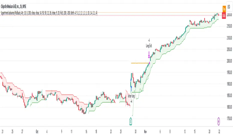
Session candles & reversals / Flowly Indicators— Overview
Like traditional candles, session based candles are a visualization of open, high, low and close values, but based on session time periods instead of typical timeframes such as daily or weekly. Session candles are formed by fetching price at session start (open), highest price during session (high), lowest price during session (low) and price at session end (close). On top of candles, session based moving average is formed and session reversals detected. Session reversals are also backtested, using win rate and magnitude metrics to better understand what to expect from session reversals and which ones have historically performed the best.
By default, following session time periods are used:
Session #1: London (08:00 - 17:00, UTC)
Session #2: New York (13:00 - 22:00, UTC)
Session #3: Sydney (21:00 - 06:00, UTC)
Session #4: Tokyo (00:00 - 09:00, UTC)
Session time periods can be changed via input menu.
— Reversals
Session reversals are patterns that show a rapid change in direction during session. These formations are more familiarly known as wicks or engulfing candles. Following criteria must be met to qualify as a session reversal:
Wick up:
Lower high, lower low, close >= 65% of session range (0% being the very low, 100% being the very high) and open >= 40% of session range.
Wick down:
Higher high, higher low, close <= 35% of session range and open <= 60% of session range.
Engulfing up:
Higher high, lower low, close >= 65% of session range.
Engulfing down:
Higher high, lower low, close <= 35% of session range.
Session reversals are always based on prior corresponding session , e.g. to qualify as a NY session engulfing up, NY session must have a higher high and lower low relative to prior NY session , not just any session that has taken place in between. Session reversals should be viewed the same way wicks/engulfing formations are viewed on traditional timeframe based candles. Essentially, wick reversals (light green/red labels) tell you most of the motion during session was reversed. Engulfing reversals (dark green/red labels) on the other hand tell you all of the motion was reversed and new direction set.
— Backtesting
Session reversals are backtested using win rate and magnitude metrics. A session reversal is considered successful when next corresponding session closes higher/lower than session reversal close . Win rate is formed by dividing successful session reversal count with total reversal count, e.g. 5 successful reversals up / 10 reversals up total = 50% win rate. Win rate tells us what are the odds (historically) of session reversal producing a clean supporting move that was persistent enough to close that way too.
When a session reversal is successful, its magnitude is measured using percentage increase/decrease from session reversal close to next corresponding session high/low . If NY session closes higher than prior NY session that was a reversal up, the percentage increase from prior session close (reversal close) to current session high is measured. If NY session closes lower than prior NY session that was a reversal down, the percentage decrease from prior session close to current session low is measured.
Average magnitude is formed by dividing all percentage increases/decreases with total reversal count, e.g. 10 total reversals up with 1% increase each -> 10% net increase from all reversals -> 10% total increase / 10 total reversals up = 1% average magnitude. Magnitude metric supports win rate by indicating the depth of successful session reversal moves.
To better understand the backtesting calculations and more importantly to verify their validity, backtesting visuals for each session can be plotted on the chart:
All backtesting results are shown in the backtesting panel on top right corner, with highest win rates and magnitude metrics for both reversals up and down marked separately. Note that past performance is not a guarantee of future performance and session reversals as they are should not be viewed as a complete strategy for long/short plays. Always make sure reversal count is sufficient to draw reliable conclusions of performance.
— Session moving average
Users can form a session based moving average with their preferred smoothing method (SMA , EMA , HMA , WMA , RMA) and length, as well as choose which sessions to include in the moving average. For example, a moving average based on New York and Tokyo sessions can be formed, leaving London and Sydney completely out of the calculation.
— Visuals
By default, script hides your candles/bars, although in the case of candles borders will still be visible. Switching to bars/line will make your regular chart visuals 100% hidden. This setting can be turned off via input menu. As some sessions overlap, each session candle can be separately offsetted forward, clearing the overlaps. Users can also choose which session candles to show/hide.
Session periods can be highlighted on the chart as a background color, applicable to only session candles that are activated. By default, session reversals are referred to as L (London), N (New York), S (Sydney) and T (Tokyo) in both reversal labels and backtesting table. By toggling on "Numerize sessions", these will be replaced with 1, 2, 3 and 4. This will be helpful when using a custom session that isn't any of the above.
Visual settings example:
Session candles are plotted in two formats, using boxes and lines as well as plotcandle() function. Session candles constructed using boxes and lines will be clear and much easier on the eyes, but will apply only to first 500 bars due to Tradingview related limitations. Rest of the session candles go back indefinitely, but won't be as clean:
All colors can be customized via input menu.
— Timeframe & session time period considerations
As a rule of thumb, session candles should be used on timeframes at or below 1H, as higher timeframes might not match with session period start/end, leading to incorrect plots. Using 1 hour timeframe will bring optimal results as greatest amount historical data is available without sacrificing accuracy of OHLC values. If you are using a custom session that is not based on hourly period (e.g. 08:00 - 15:00 vs. 08.00 - 15.15) make sure you are using a timeframe that allows correct plots.
Session time periods applied by default are rough estimates and might be out of bounds on some charts, like NYSE listed equities. This is rarely a problem on assets that have extensive trading hours, like futures or cryptocurrency. If a session is out of bounds (asset isn't traded during the set session time period) the script won't plot given session candle and its backtesting metrics will be NA. This can be fixed by changing the session time periods to match with given asset trading hours, although you will have to consider whether or not this defeats the purpose of having candles based on sessions.
— Practical guide
Whether based on traditional timeframes or sessions, reversals should always be considered as only one piece of evidence of price turning. Never react to them without considering other factors that might support the thesis, such as levels and multi-timeframe analysis. In short, same basic charting principles apply with session candles that apply with normal candles. Use discretion.
Example #1 : Focusing efforts on session reversals at distinct support/resistance levels
A reversal against a level holds more value than a reversal by itself, as you know it's a placement where liquidity can be expected. A reversal serves as a confirming reaction for this expectation.
Example #2 : Focusing efforts on highest performing reversals and avoiding poorly performing ones
As you have data backed evidence of session reversal performance, it makes sense to focus your efforts on the ones that perform best. If some session reversal is clearly performing poorly, you would want to avoid it, since there's nothing backing up its validity.
Example #3 : Reversal clusters
Two is better than one, three is better than two and so on. If there are rapid changes in direction within multiple sessions consecutively, there's heavier evidence of a dynamic shift in price. In such case, it makes sense to hold more confidence in price halting/turning.

Squeeze Momentum Strategy [LazyBear] Buy Sell TP SL Alerts-Modified version of Squeeze Momentum Indicator by @LazyBear.
-Converted to version 5,
-Taken inspiration from @KivancOzbilgic for its buy sell calculations,
-Used @Bunghole strategy template with Take Profit, Stop Loss and Enable/Disable Toggles
-Added Custom Date Backtesting Module
------------------------------------------------------------------------------------------------------------------------
All credit goes to above
Problem with original version:
The original Squeeze Momentum Strategy did not have buy sell signals and there was alot of confusion as to when to enter and exit.
There was no proper strategy that would allow backtesting on which further analysis could be carried out.
There are 3 aspects this strategy:
1 ) Strategy Logic (easily toggleable from the dropdown menu from strategy settings)
- LazyBear (I have made this simple by using Kivanc technique of Momentums Moving Average Crossover, BUY when MA cross above signal line, SELL when crossdown signal line)
- Zero Crossover Line (BUY signal when crossover zero line, and SELL crossdown zero line)
2) Long Short TP and SL
- In strategies there is usually only 1 SL and 1 TP, and it is assumed that if a 2% SL giving a good profit %, then it would be best for both long and short. However this is not the case for many. Many markets/pairs, go down with much more speed then they go up with. Hence once we have a profitable backtesting setting, then we should start optimizing Long and Short SL's seperately. Once that is done, we should start optimizing for Long and Short TP's separately, starting with Longs first in both cases.
3) Enable and Disable Toggles of Long and Short Trades
- Many markets dont allow short trades, or are not suitable for short trades. In this case it would be much more feasible to disable "Short" Trading and see results of Long Only as a built in graphic view of backtestor provides a more easy to understand data feed as compared to the performance summary in which you have to review long and short profitability separately.
4) Custom Data Backtesting
- One of most crucial aspects while optimizing for backtesting is to check a strategies performance on uptrends, downtrend and sideways markets seperately as to understand the weak points of strategy.
- Once you enable custom date backtesting, you will see lines on the chart which can be dragged left right based on where you want to start and end the backtesting from and to.
Note:
- Not a financial advise
- Open to feedback, questions, improvements, errors etc.
- More info on how the squeeze momentum works visit LazyBear indicator link:
Happy Trading!
Cheers
M Tahreem Alam @mtahreemalam
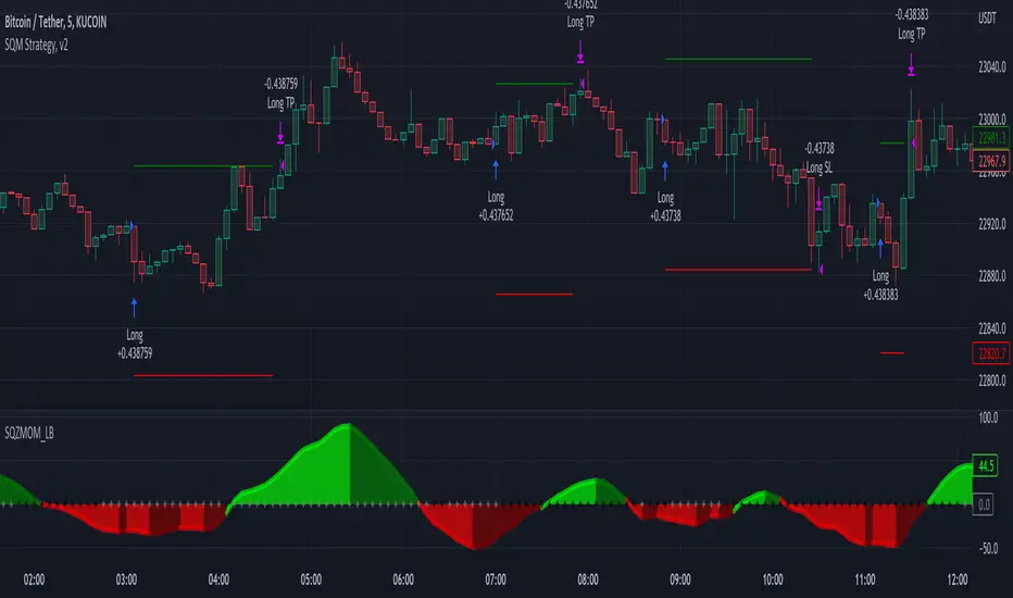
ORB FX REPLAY - FINAL SAFEHere is the description in English, written to sound professional and meet all the requirements for publishing on TradingView:
Script Description:
Title: ORB Strategy Backtest Pro - Ultra Compatibility
Description: This is an Opening Range Breakout (ORB) strategy specifically designed for professional backtesting. It is optimized to run smoothly on external platforms like FX Replay and TradingView's replay mode.
Key Features:
Custom Session: Automatically calculates the High and Low of a specific time window (default: 10:00 - 10:15 Bucharest/GMT+2).
Impulse Confirmation: Features a "Min Impulse" filter to ensure entries happen on strong momentum, avoiding "fake-outs" near the range boundaries.
Hard Target Management: Designed for "Set & Forget" backtesting. Once a trade is triggered, the script tracks it until it hits either the Stop Loss (SL) or the final Take Profit 3 (TP3).
Visual Projections: Draws clear, real-time lines for Entry, SL, and TP3 on the chart for easy visual tracking.
Automated Statistics: Includes a dynamic label system that tracks Total Trades, Win Count, and Loss Count based on the TP3/SL logic.
Optimized Code: Built using Pine Script v5 with a focus on stability and compatibility, avoiding complex tables that often cause errors on external engines.

Optimized ADX DI CCI Strategy### Key Features:
- Combines ADX, DI+/-, CCI, and RSI for signal generation.
- Supports customizable timeframes for indicators.
- Offers multiple exit conditions (Moving Average cross, ADX change, performance-based stop-loss).
- Tracks and displays trade statistics (e.g., win rate, capital growth, profit factor).
- Visualizes trades with labels and optional background coloring.
- Allows countertrading (opening an opposite trade after closing one).
1. **Indicator Calculation**:
- **ADX and DI+/-**: Calculated using the `ta.dmi` function with user-defined lengths for DI and ADX smoothing.
- **CCI**: Computed using the `ta.cci` function with a configurable source (default: `hlc3`) and length.
- **RSI (optional)**: Calculated using the `ta.rsi` function to filter overbought/oversold conditions.
- **Moving Averages**: Used for CCI signal smoothing and trade exits, with support for SMA, EMA, SMMA (RMA), WMA, and VWMA.
2. **Signal Generation**:
- **Buy Signal**: Triggered when DI+ > DI- (or DI+ crosses over DI-), CCI > MA (or CCI crosses over MA), and optional ADX/RSI filters are satisfied.
- **Sell Signal**: Triggered when DI+ < DI- (or DI- crosses over DI+), CCI < MA (or CCI crosses under MA), and optional ADX/RSI filters are satisfied.
3. **Trade Execution**:
- **Entry**: Long or short trades are opened using `strategy.entry` when signals are detected, provided trading is allowed (`allow_long`/`allow_short`) and equity is positive.
- **Exit**: Trades can be closed based on:
- Opposite signal (if no other exit conditions are used).
- MA cross (price crossing below/above the exit MA for long/short trades).
- ADX percentage change exceeding a threshold.
- Performance-based stop-loss (trade loss exceeding a percentage).
- **Countertrading**: If enabled, closing a trade triggers an opposite trade (e.g., closing a long opens a short).
4. **Visualization**:
- Labels are plotted at trade entries/exits (e.g., "BUY," "SELL," arrows).
- Optional background coloring highlights open trades (green for long, red for short).
- A statistics table displays real-time metrics (e.g., capital, win rates).
5. **Trade Tracking**:
- Tracks the number of long/short trades, wins, and overall performance.
- Monitors equity to prevent trading if it falls to zero.
### 2.3 Key Components
- **Indicator Calculations**: Uses `request.security` to fetch indicator data for the specified timeframe.
- **MA Function**: A custom `ma_func` handles different MA types for CCI and exit conditions.
- **Signal Logic**: Combines crossover/under checks with recent bar windows for flexibility.
- **Exit Conditions**: Multiple configurable exit strategies for risk management.
- **Statistics Table**: Updates dynamically with trade and capital metrics.
## 3. Configuration Options
The script provides extensive customization through input parameters, grouped for clarity in the TradingView settings panel. Below is a detailed breakdown of each setting and its impact.
### 3.1 Strategy Settings (Global)
- **Initial Capital**: Default `10000`. Sets the starting capital for backtesting.
- **Effect**: Determines the base equity for calculating position sizes and performance metrics.
- **Default Quantity Type**: `strategy.percent_of_equity` (50% of equity).
- **Effect**: Controls the size of each trade as a percentage of available equity.
- **Pyramiding**: Default `2`. Allows up to 2 simultaneous trades in the same direction.
- **Effect**: Enables multiple entries if conditions are met, increasing exposure.
- **Commission**: 0.2% per trade.
- **Effect**: Simulates trading fees, reducing net profit in backtesting.
- **Margin**: 100% for long and short trades.
- **Effect**: Assumes no leverage; adjust for margin trading simulations.
- **Calc on Every Tick**: `true`.
- **Effect**: Ensures real-time signal updates for precise execution.
### 3.2 Indicator Settings
- **Indicator Timeframe** (`indicator_timeframe`):
- **Options**: `""` (chart timeframe), `1`, `5`, `15`, `30`, `60`, `240`, `D`, `W`.
- **Default**: `""` (uses chart timeframe).
- **Effect**: Determines the timeframe for ADX, DI, CCI, and RSI calculations. A higher timeframe reduces noise but may delay signals.
### 3.3 ADX & DI Settings
- **DI Length** (`adx_di_len`):
- **Default**: `30`.
- **Range**: Minimum `1`.
- **Effect**: Sets the period for calculating DI+ and DI-. Longer periods smooth trends but reduce sensitivity.
- **ADX Smoothing Length** (`adx_smooth_len`):
- **Default**: `14`.
- **Range**: Minimum `1`.
- **Effect**: Smooths the ADX calculation. Longer periods produce smoother ADX values.
- **Use ADX Filter** (`use_adx_filter`):
- **Default**: `false`.
- **Effect**: If `true`, requires ADX to exceed the threshold for signals to be valid, filtering out weak trends.
- **ADX Threshold** (`adx_threshold`):
- **Default**: `25`.
- **Range**: Minimum `0`.
- **Effect**: Sets the minimum ADX value for valid signals when the filter is enabled. Higher values restrict trades to stronger trends.
### 3.4 CCI Settings
- **CCI Length** (`cci_length`):
- **Default**: `20`.
- **Range**: Minimum `1`.
- **Effect**: Sets the period for CCI calculation. Longer periods reduce noise but may lag.
- **CCI Source** (`cci_src`):
- **Default**: `hlc3` (average of high, low, close).
- **Effect**: Defines the price data for CCI. `hlc3` is standard, but users can choose other sources (e.g., `close`).
- **CCI MA Type** (`ma_type`):
- **Options**: `SMA`, `EMA`, `SMMA (RMA)`, `WMA`, `VWMA`.
- **Default**: `SMA`.
- **Effect**: Determines the moving average type for CCI signal smoothing. EMA is more responsive; VWMA weights by volume.
- **CCI MA Length** (`ma_length`):
- **Default**: `14`.
- **Range**: Minimum `1`.
- **Effect**: Sets the period for the CCI MA. Longer periods smooth the MA but may delay signals.
### 3.5 RSI Filter Settings
- **Use RSI Filter** (`use_rsi_filter`):
- **Default**: `false`.
- **Effect**: If `true`, applies RSI-based overbought/oversold filters to signals.
- **RSI Length** (`rsi_length`):
- **Default**: `14`.
- **Range**: Minimum `1`.
- **Effect**: Sets the period for RSI calculation. Longer periods reduce sensitivity.
- **RSI Lower Limit** (`rsi_lower_limit`):
- **Default**: `30`.
- **Range**: `0` to `100`.
- **Effect**: Defines the oversold threshold for buy signals. Lower values allow trades in more extreme conditions.
- **RSI Upper Limit** (`rsi_upper_limit`):
- **Default**: `70`.
- **Range**: `0` to `100`.
- **Effect**: Defines the overbought threshold for sell signals. Higher values allow trades in more extreme conditions.
### 3.6 Signal Settings
- **Cross Window** (`cross_window`):
- **Default**: `0`.
- **Range**: `0` to `5` bars.
- **Effect**: Specifies the lookback period for detecting DI+/- or CCI crosses. `0` requires crosses on the current bar; higher values allow recent crosses, increasing signal frequency.
- **Allow Long Trades** (`allow_long`):
- **Default**: `true`.
- **Effect**: Enables/disables new long trades. If `false`, only closing existing longs is allowed.
- **Allow Short Trades** (`allow_short`):
- **Default**: `true`.
- **Effect**: Enables/disables new short trades. If `false`, only closing existing shorts is allowed.
- **Require DI+/DI- Cross for Buy** (`buy_di_cross`):
- **Default**: `true`.
- **Effect**: If `true`, requires a DI+ crossover DI- for buy signals; if `false`, DI+ > DI- is sufficient.
- **Require CCI Cross for Buy** (`buy_cci_cross`):
- **Default**: `true`.
- **Effect**: If `true`, requires a CCI crossover MA for buy signals; if `false`, CCI > MA is sufficient.
- **Require DI+/DI- Cross for Sell** (`sell_di_cross`):
- **Default**: `true`.
- **Effect**: If `true`, requires a DI- crossover DI+ for sell signals; if `false`, DI+ < DI- is sufficient.
- **Require CCI Cross for Sell** (`sell_cci_cross`):
- **Default**: `true`.
- **Effect**: If `true`, requires a CCI crossunder MA for sell signals; if `false`, CCI < MA is sufficient.
- **Countertrade** (`countertrade`):
- **Default**: `true`.
- **Effect**: If `true`, closing a trade triggers an opposite trade (e.g., close long, open short) if allowed.
- **Color Background for Open Trades** (`color_background`):
- **Default**: `true`.
- **Effect**: If `true`, colors the chart background green for long trades and red for short trades.
### 3.7 Exit Settings
- **Use MA Cross for Exit** (`use_ma_exit`):
- **Default**: `true`.
- **Effect**: If `true`, closes trades when the price crosses the exit MA (below for long, above for short).
- **MA Length for Exit** (`ma_exit_length`):
- **Default**: `20`.
- **Range**: Minimum `1`.
- **Effect**: Sets the period for the exit MA. Longer periods delay exits.
- **MA Type for Exit** (`ma_exit_type`):
- **Options**: `SMA`, `EMA`, `SMMA (RMA)`, `WMA`, `VWMA`.
- **Default**: `SMA`.
- **Effect**: Determines the MA type for exit signals. EMA is more responsive; VWMA weights by volume.
- **Use ADX Change Stop-Loss** (`use_adx_stop`):
- **Default**: `false`.
- **Effect**: If `true`, closes trades when the ADX changes by a specified percentage.
- **ADX % Change for Stop-Loss** (`adx_change_percent`):
- **Default**: `5.0`.
- **Range**: Minimum `0.0`, step `0.1`.
- **Effect**: Specifies the percentage change in ADX (vs. previous bar) that triggers a stop-loss. Higher values reduce premature exits.
- **Use Performance Stop-Loss** (`use_perf_stop`):
- **Default**: `false`.
- **Effect**: If `true`, closes trades when the loss exceeds a percentage threshold.
- **Performance Stop-Loss (%)** (`perf_stop_percent`):
- **Default**: `-10.0`.
- **Range**: `-100.0` to `0.0`, step `0.1`.
- **Effect**: Specifies the loss percentage that triggers a stop-loss. More negative values allow larger losses before exiting.
## 4. Visual and Statistical Output
- **Labels**: Displayed at trade entries/exits with arrows (↑ for buy, ↓ for sell) and text ("BUY," "SELL"). A "No Equity" label appears if equity is zero.
- **Background Coloring**: Optionally colors the chart background (green for long, red for short) to indicate open trades.
- **Statistics Table**: Displayed at the top center of the chart, updated on timeframe changes or trade events. Includes:
- **Capital Metrics**: Initial capital, current capital, capital growth (%).
- **Trade Metrics**: Total trades, long/short trades, win rate, long/short win rates, profit factor.
- **Open Trade Status**: Indicates if a long, short, or no trade is open.
## 5. Alerts
- **Buy Signal Alert**: Triggered when `buy_signal` is true ("Cross Buy Signal").
- **Sell Signal Alert**: Triggered when `sell_signal` is true ("Cross Sell Signal").
- **Usage**: Users can set up TradingView alerts to receive notifications for trade signals.
