Microstructure Participation & Acceptance Indicator📊 Microstructure Participation & Acceptance Indicator
An advanced participation-based filter combining VWAP distance analysis, volume delta detection, and real-time acceptance/rejection state identification—designed for smaller timeframe trading.
📊 FEATURES
VWAP Distance Normalization
Context-aware fair value measurement:
Automatically resets based on selected anchor (Session/Week/Month)
ATR-normalized distance calculation for universal application
Identifies when price is extended or compressed relative to equilibrium
Configurable extreme distance threshold (default: 1.5 ATR)
Adjustable source input (default: HLC3)
Volume Delta Proxy
Bull vs Bear participation tracking:
Calculates volume imbalance between bullish and bearish candles
EMA smoothing for cleaner signal generation (default: 9 periods)
Delta ratio measurement to identify dominant side
Expansion/compression detection to gauge momentum commitment
Configurable expansion threshold (default: 1.3x)
Acceptance/Rejection State Machine
Real-time market regime identification with six distinct states:
🟢 Accepted Long
Price moving away from VWAP with expanding bullish delta
Distance from VWAP increasing
Volume confirming the move
Indicates real buying pressure—trade WITH the move
🟢 Accepted Short
Price moving away from VWAP with expanding bearish delta
Distance from VWAP increasing
Volume confirming the move
Indicates real selling pressure—trade WITH the move
🟠 Fade Long
Price extended beyond threshold (>1.5 ATR above VWAP)
Delta not supporting the extension
Volume participation absent or diminishing
Potential mean-reversion short setup
🟠 Fade Short
Price extended beyond threshold (>1.5 ATR below VWAP)
Delta not supporting the extension
Volume participation absent or diminishing
Potential mean-reversion long setup
⚪ Chop
Price compressed near VWAP
Bollinger Bands tight (width compressed)
Delta neutral—no clear commitment
NO TRADE ZONE—wait for expansion
⚪ Neutral
Transitional state between regimes
Momentum shifting but not yet confirmed
Monitor for next acceptance signal
Bollinger Bands
Standard volatility measurement with TradingView default styling:
Adjustable period length (default: 20)
Configurable standard deviation multiplier (default: 2.0)
Visual fill between bands for volatility context
Used internally for chop/compression detection
Live Dashboard
Real-time metrics display (top-right corner):
Current market state with color coding
VWAP distance in ATR units
Delta ratio (bull/bear volume balance)
Delta state (Expanding/Compressing)
High-contrast design for instant readability
🎯 HOW TO USE
For Trend Trading:
Accepted Long/Short backgrounds indicate confirmed participation—stay with the trend
Strong moves typically travel 1-1.5 ATR from VWAP with delta support
Use VWAP as dynamic support/resistance
Combine with momentum indicators (MACD, RSI) for confluence
Price above VWAP + Accepted Long state = bullish bias
Price below VWAP + Accepted Short state = bearish bias
For Mean Reversion:
Fade Long/Short states signal overextension without participation
Price beyond 1.5 ATR from VWAP with weak delta = potential reversal
Look for price return to VWAP when extended
Bollinger Band extremes + Fade state = high-probability mean reversion setup
VWAP acts as mean reversion anchor during range-bound sessions
For Risk Management:
Chop state = avoid new entries
Bollinger Band compression + Chop = pre-expansion zone (wait for breakout)
Delta compression after strong move = early exhaustion warning
State transitions (Accepted → Neutral → Fade) = tighten stops
Signal Confirmation:
Strongest setups occur when multiple factors align:
BB breakout + Accepted state + price above/below VWAP
Price rejection at BB bands + Fade state
VWAP support/resistance hold + state transition
Delta expansion + distance increasing + trend direction
⚙️ SETTINGS
All components are fully customizable through organized input groups:
VWAP Distance Group:
VWAP source (default: HLC3)
Anchor period (Session/Week/Month)
ATR length for normalization (default: 14)
Extreme distance threshold in ATR multiples (default: 1.5)
Volume Delta Group:
Delta EMA length (default: 9)
Delta expansion threshold (default: 1.3)
Acceptance Logic Group:
Acceptance lookback period (default: 5)
Chop threshold in VWAP/ATR units (default: 0.3)
Bollinger Bands Group:
BB length (default: 20)
Standard deviation multiplier (default: 2.0)
Display Group:
Toggle state backgrounds
Toggle state change labels
Toggle VWAP line
Toggle Bollinger Bands
💡 EDUCATIONAL VALUE
This indicator teaches important concepts:
How institutional money identifies fair value (VWAP)
The difference between price movement and market acceptance
Why volume participation matters more than price action alone
How to distinguish between noise and committed directional moves
The relationship between volatility compression and expansion cycles
Why distance from equilibrium predicts mean reversion probability
⚠️ IMPORTANT NOTES
This indicator is for educational and informational purposes only
This is a filter, not a standalone trading system
No indicator is perfect—always use proper risk management
Past performance does not guarantee future results
Combine with your own analysis and risk tolerance
Test thoroughly on historical data before live trading
This is not financial advice—use at your own risk
🔧 TECHNICAL DETAILS
Pine Script Version 6
Overlay indicator (displays on price chart)
All calculations use standard, well-documented formulas
No repainting—all signals are confirmed on bar close
Compatible with all timeframes and instruments
Optimized for smaller timeframes (1-5 minute charts)
Minimal computational overhead
📝 CHANGELOG
Version 1.0
Initial release
VWAP distance normalization with ATR scaling
Volume delta proxy system (bull/bear EMA)
6-state acceptance/rejection state machine
Bollinger Bands integration
Real-time dashboard with live metrics
State change labels and background coloring
Full customization options
Developed for traders who need objective participation filters to distinguish high-probability setups from low-quality noise—without cluttering their charts with multiple indicator panels.
Cerca negli script per "bear"

AI-based Price action confluence dashboard# **AI-Based Price Action Confluence Dashboard - Publication Guide**
Here's a comprehensive introduction guide for your TradingView indicator publication:
***
## **📊 TITLE**
**AI-Based Price Action Confluence Dashboard**
***
## **🎯 SHORT DESCRIPTION** (For the summary field)
A sophisticated real-time confluence scoring system that analyzes multiple price action signals across 15-minute timeframes, providing traders with an AI-weighted scoring mechanism (0-6 scale) to identify high-probability trade setups through visual signal panels and intelligent path detection.
***
## **📝 FULL DESCRIPTION**
### **Overview**
The AI-Based Price Action Confluence Dashboard is an advanced technical indicator designed to eliminate guesswork in intraday trading by systematically scoring and displaying multiple price action signals in real-time. Unlike traditional single-indicator approaches, this dashboard employs a confluence methodology that combines multiple independent signals to provide stronger trade confirmations and reduce false signals.
This indicator is specifically optimized for **1-minute chart analysis** while monitoring **15-minute price structure**, making it ideal for day traders and scalpers who need precise entry timing with larger timeframe context.
***
### **🔑 Key Features**
**✅ Real-Time AI Confluence Scoring**
- Dynamic scoring system (0-6 points) for both bullish and bearish setups
- Visual meter display shows signal strength at a glance
- Color-coded backgrounds indicate confluence levels (strong, moderate, mixed)
**✅ Multi-Signal Analysis**
The dashboard tracks 6 distinct signal types:
1. **FTFC (First to Finish Close)** - Base & Bonus signals
2. **Long/Short Grab** - Liquidity sweep patterns (Path A)
3. **High/Low Hold** - Extended momentum confirmation (+2 bonus)
4. **2-Up/2-Down** - Clean breakout patterns (Path B)
5. **Breakaway** - First candle gap strategies
**✅ Intelligent Path Detection**
- Mutually exclusive path logic prevents signal conflicts
- Automatically identifies whether price is following a "sweep path" or "clean path"
- Unavailable paths are clearly marked with gray indicators
**✅ Visual Signal Panels**
- 🟢 Green Light = Bullish signal ACTIVE
- 🔴 Red Light = Bearish signal ACTIVE
- 🟡 Yellow Light = Signal BUILDING (conditions partially met)
- ⚪ White Light = Signal OFF
- ▪️ Gray Square = Path UNAVAILABLE (mutually exclusive)
**✅ Comprehensive Alert System**
- 10 different alert conditions covering all major signals
- Strong confluence alerts (5+ points)
- Individual signal completion alerts
- Customizable alert messages
***
### **📐 How It Works**
#### **The Confluence Methodology**
This indicator implements a sophisticated confluence trading approach where multiple independent price action signals are combined to identify high-probability setups. Each signal type contributes points to either the bullish or bearish score, with a maximum of 6 points per direction.
**Scoring Breakdown:**
**BULLISH SIGNALS:**
- FTFC Base (15m close > previous 15m close) = +1
- FTFC Bonus (price clears 15th candle high) = +1
- **PATH A (Sweep):** Long Grab = +1, High Hold Bonus = +2
- **PATH B (Clean):** 2-Up = +1, 2-Up Bonus = +1
- Breakaway (gap above first candle) = +1
**BEARISH SIGNALS:**
- FTFC Base (15m close < previous 15m close) = +1
- FTFC Bonus (price clears 15th candle low) = +1
- **PATH A (Sweep):** Short Grab = +1, Low Hold Bonus = +2
- **PATH B (Clean):** 2-Down = +1, 2-Down Bonus = +1
- Breakaway (gap below first candle) = +1
#### **Path Detection Logic**
The indicator automatically determines which path the market is following:
**PATH A: SWEEP PATH**
- Activated when previous 15m low (bull) or high (bear) is breached
- Indicates liquidity grab before reversal
- Includes powerful +2 bonus for "Hold" confirmations
- Mutually exclusive with Path B
**PATH B: CLEAN PATH**
- Activated when previous 15m low (bull) or high (bear) holds
- Indicates strong directional momentum without sweep
- Cleaner price action but smaller point potential
- Mutually exclusive with Path A
This mutual exclusivity prevents double-counting and ensures signal accuracy.
***
### **🎨 How to Use**
#### **Installation**
1. Add indicator to your 1-minute chart
2. The dashboard appears as a table overlay (default: top right)
3. No additional indicators required - this is a complete system
#### **Reading the Dashboard**
**Top Section - Confluence Meter:**
- Shows current bull/bear scores with visual dot meters
- Background color changes based on confluence strength:
- **Bright Green/Red** = 5+ points (strong directional bias)
- **Medium Green/Red** = 3+ points (moderate bias)
- **Orange** = 3+ points both sides (conflicting signals)
- **Gray** = Low confluence (choppy conditions)
**Signal Panels Section:**
- Each row shows a signal type with bull/bear lights side-by-side
- Active signals (🟢🔴) contribute to the total score
- Building signals (🟡) indicate potential setups forming
- Unavailable paths (▪️) show which exclusive path is blocked
#### **Trading Strategy**
**High-Probability Long Entries:**
- Bull score ≥ 5 AND bear score ≤ 1
- Multiple green lights active in signal panels
- PATH A or PATH B showing full completion
- Consider entry on pullback to key 15m level
**High-Probability Short Entries:**
- Bear score ≥ 5 AND bull score ≤ 1
- Multiple red lights active in signal panels
- PATH A or PATH B showing full completion
- Consider entry on rally to key 15m level
**Avoid Trading When:**
- Both scores are 3+ (conflicting signals)
- No path is showing active/building status
- Score is below 3 on both sides (low confluence)
#### **Risk Management**
- Use 15m swing high/low for stop placement
- Target opposing 15m level or previous session extremes
- Scale out at partial targets when confluence decreases
- Best results when combined with proper position sizing
***
### **⚙️ Customization**
**Dashboard Settings:**
- **Table Location:** Top Left, Top Right, Bottom Left, Bottom Right
- **Text Size:** Tiny, Small, Normal, Large
**Color Scheme:**
- **Bullish Color:** Customize green for bull signals (default: #00cc66)
- **Bearish Color:** Customize red for bear signals (default: #ff4444)
- **Building Color:** Customize yellow for forming signals (default: #ffaa00)
- **Inactive Color:** Customize gray for off signals (default: #555555)
- **Unavailable Color:** Customize dark gray for blocked paths (default: #333333)
All colors can be adjusted to match your chart theme or visual preferences.
***
### **🎯 Best Practices**
1. **Use on 1-minute charts only** - The indicator is calibrated for this timeframe
2. **Trade during liquid sessions** - Best results during NY/London overlap
3. **Wait for 3+ confluence** - Minimum threshold for trade consideration
4. **Watch path transitions** - Signal strength changes when paths flip
5. **Use alerts strategically** - Set alerts for 5+ confluence to catch strong setups
6. **Combine with volume** - High volume confirms signal validity
7. **Respect 15m structure** - Don't fight the larger timeframe bias
***
### **⚠️ Important Notes**
- This indicator is designed for **intraday trading only**
- Requires active monitoring during trading sessions
- Works best on liquid instruments (major forex pairs, indices, large-cap stocks)
- Not suitable for swing trading or position trading
- Past performance does not guarantee future results
- Always use proper risk management and position sizing
***
### **🏷️ Category**
**Oscillators** or **Volatility** (choose based on TradingView categories)
***
### **🏷️ Suggested Tags**
- confluence
- price action
- day trading
- scalping
- intraday
- signals
- dashboard
- multi-timeframe
- 1-minute
- 15-minute
***
### **📜 Disclaimer**
This indicator is a tool for technical analysis and should not be used as the sole basis for trading decisions. All trading involves risk, and you should never risk more than you can afford to lose. The developer assumes no responsibility for trading losses incurred through the use of this indicator. Always practice proper risk management and consider your own risk tolerance before trading.

Hybrid Strategy: Trend/ORB/MTFHybrid Strategy: Trend + ORB + Multi-Timeframe Matrix
This script is a comprehensive "Trading Manager" designed to filter out noise and identify high-probability breakout setups. It combines three powerful concepts into a single, clean chart interface: Trend Alignment, Opening Range Breakout (ORB), and Multi-Timeframe (MTF) Analysis.
It is designed to prevent "analysis paralysis" by providing a unified Dashboard that confirms if the trend is aligned across 5 different timeframes before you take a trade.
How it Works
The strategy relies on the "Golden Trio" of confluence:
1. Trend Definition (The Setup) Before looking for entries, the script analyzes the immediate trend. A bullish trend is defined as:
Price is above the Session VWAP.
The fast EMA (9) is above the slow EMA (21). (The inverse applies for bearish trends).
2. The Signal (The Trigger) The script draws the Opening Range (default: first 15 minutes of the session).
Buy Signal: Price breaks above the Opening Range High while the Trend is Bullish.
Sell Signal: Price breaks below the Opening Range Low while the Trend is Bearish.
3. The Confirmation (The Filter) A signal is only valid if the Higher Timeframe (default: 60m) agrees with the direction. If the 1m chart says "Buy" but the 60m chart is bearish, the signal is filtered out to prevent false breakouts.
Key Features
The Matrix Dashboard A zero-lag, real-time table in the corner of your screen that monitors 5 user-defined timeframes (e.g., 5m, 15m, 30m, 60m, 4H).
Trend: Checks if Price > EMA 21.
VWAP: Checks if Price > VWAP.
ORB: Checks if Price is currently above/below the Opening Range of that session.
D H/L: Warns if price is near the Daily High or Low.
PD H/L: Warns if price is near the Previous Daily High or Low.
Visual Order Blocks The script automatically identifies valid Order Blocks (sequences of consecutive candles followed by a strong explosive move).
Chart: Draws Green/Red zones extending to the right, showing where price may react.
Dashboard: Displays the exact High, Low, and Average price of the most recent Order Blocks for precision planning.
Risk Management (Trailing Stop) Once a trade is active, the script plots Chandelier Exit dots (ATR-based trailing stop) to help you manage the trade and lock in profits during trend runs.
Visual Guide (Chart Legend)
⬜ Gray Box: Represents the Opening Range (first 15 minutes). This is your "No Trade Zone." Wait for price to break out of this box.
🟢 Green Line: The Opening Range High. A break above this line signals potential Bullish momentum.
🔴 Red Line: The Opening Range Low. A break below this line signals potential Bearish momentum.
🟢 Green / 🔴 Red Zones (Boxes): These are Order Blocks.
🟢 Green Zone: A Bullish Order Block (Demand). Expect price to potentially bounce up from here.
🔴 Red Zone: A Bearish Order Block (Supply). Expect price to potentially reject down from here.
⚪ Dots (Trailing Stop):
🟢 Green Dots: These appear below price during a Bullish trend. They represent your suggested Stop Loss.
🔴 Red Dots: These appear above price during a Bearish trend.
🏷️ Buy / Sell Labels:
BUY: Triggers when Price breaks the Green Line + Trend is Bullish + HTF is Bullish.
SELL: Triggers when Price breaks the Red Line + Trend is Bearish + HTF is Bearish.
Settings
Session: Customizable RTH (Regular Trading Hours) to filter out pre-market noise.
Matrix Timeframes: 5 fixed slots to choose which timeframes you want to monitor.
Order Blocks: Adjust the sensitivity and lookback period for Order Block detection.
Risk: Customize the ATR multiplier for the trailing stop.
Disclaimer
This tool is for educational purposes only. Past performance does not guarantee future results. Always manage your risk properly.

VR Volume Ratio + Divergence (Pro)成交量比率 (Volume Ratio, VR) 是一項通過分析股價上漲與下跌日的成交量,來研判市場資金氣氛的技術指標。本腳本基於傳統 VR 公式進行了優化,增加了**「趨勢變色」與「自動背離偵測」**功能,幫助交易者更精準地捕捉量價轉折點。
Introduction
Volume Ratio (VR) is a technical indicator that measures the strength of a trend by comparing the volume on up-days versus down-days. This script enhances the classic VR formula with "Trend Color Coding" and "Auto-Divergence Detection", helping traders identify volume-price reversals more accurately.
核心功能與參數
公式原理: VR = (Qu + Qf/2) / (Qd + Qf/2) * 100
Qu: 上漲日成交量 (Up volume)
Qd: 下跌日成交量 (Down volume)
Qf: 平盤日成交量 (Flat volume)
參數 (Length):預設為 26 日,這是市場公認最有效的短中線參數。
關鍵水位線 (Key Levels):
< 40% (底部區):量縮極致,市場情緒冰點,常對應股價底部,適合尋找買點。
100% (中軸):多空分界線。
> 260% (多頭警戒):進入強勢多頭行情,但需注意過熱。
> 450% (頭部區):成交量過大,市場情緒亢奮,通常為頭部訊號。
視覺優化 (Visuals):
紅漲綠跌:當 VR 數值大於前一日顯示為紅色(動能增強);小於前一日顯示為綠色(動能退潮)。
背離訊號 (Divergence):自動標記量價背離。
▲ 底背離 (Bullish):股價創新低,但 VR 指標墊高(主力吸籌)。
▼ 頂背離 (Bearish):股價創新高,但 VR 指標走弱(買氣衰竭)。
Features & Settings
Formula Logic: Calculated as VR = (Qu + Qf/2) / (Qd + Qf/2) * 100.
Default Length: 26, widely regarded as the optimal setting for short-to-medium term analysis.
Key Zones:
< 40% (Oversold/Bottom): Extreme low volume, often indicating a market bottom and potential buying opportunity.
100% (Neutral): The balance point between bulls and bears.
> 260% (Bullish Zone): Strong uptrend, volume is expanding.
> 450% (Overbought/Top): Extreme high volume, often indicating a market top and potential reversal.
Visual Enhancements:
Color Coding: Line turns Red when VR rises (Momentum Up) and Green when VR falls (Momentum Down).
Divergence Signals: Automatically marks divergence points on the chart.
▲ Bullish Divergence: Price makes a lower low, but VR makes a higher low (Accumulation).
▼ Bearish Divergence: Price makes a higher high, but VR makes a lower high (Distribution).
應用策略建議
抄底策略:當 VR 跌破 40% 後,指標線由綠翻紅,或出現「▲底背離」訊號時,為極佳的波段進場點。
逃頂策略:當 VR 衝過 450% 進入高檔區,一旦指標線由紅翻綠,或出現「▼頂背離」訊號時,建議分批獲利了結。
Strategy Guide
Bottom Fishing: Look for entries when VR drops below 40% and turns red, or when a "▲ Bullish Divergence" label appears.
Taking Profit: Consider selling when VR exceeds 450% and turns green, or when a "▼ Bearish Divergence" label appears.
Disclaimer: This tool is for informational purposes only and does not constitute financial advice. / 本腳本僅供參考,不構成投資建議。

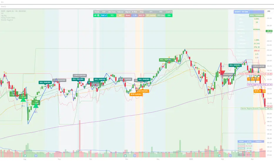
Market Regime# MARKET REGIME IDENTIFICATION & TRADING SYSTEM
## Complete User Guide
---
## 📋 TABLE OF CONTENTS
1. (#overview)
2. (#regimes)
3. (#indicator-usage)
4. (#entry-signals)
5. (#exit-signals)
6. (#regime-strategies)
7. (#confluence)
8. (#backtesting)
9. (#optimization)
10. (#examples)
---
## OVERVIEW
### What This System Does
This is a **complete market regime identification and trading system** that:
1. **Identifies 6 distinct market regimes** automatically
2. **Adapts trading tactics** to each regime
3. **Provides high-probability entry signals** with confluence scoring
4. **Shows optimal exit points** for each trade
5. **Can be backtested** to validate performance
### Two Components Provided
1. **Indicator** (`market_regime_indicator.pine`)
- Visual regime identification
- Entry/exit signals on chart
- Dynamic support/resistance
- Info tables with live data
- Use for manual trading
2. **Strategy** (`market_regime_strategy.pine`)
- Fully automated backtestable version
- Same logic as indicator
- Position sizing and risk management
- Performance metrics
- Use for backtesting and automation
---
## THE 6 MARKET REGIMES
### 1. 🟢 BULL TRENDING
**Characteristics:**
- Strong uptrend
- Price above SMA50 and SMA200
- ADX > 25 (strong trend)
- Higher highs and higher lows
- DI+ > DI- (bullish momentum)
**What It Means:**
- Market has clear upward direction
- Buyers in control
- Pullbacks are buying opportunities
- Strongest regime for long positions
**How to Trade:**
- ✅ **BUY dips to EMA20 or SMA20**
- ✅ Enter when RSI < 60 on pullback
- ✅ Hold through minor corrections
- ❌ Don't short against the trend
- ❌ Don't sell too early
**Expected Behavior:**
- Pullbacks are shallow (5-10%)
- Bounces are strong
- Support at moving averages holds
- Volume increases on rallies
---
### 2. 🔴 BEAR TRENDING
**Characteristics:**
- Strong downtrend
- Price below SMA50 and SMA200
- ADX > 25 (strong trend)
- Lower highs and lower lows
- DI- > DI+ (bearish momentum)
**What It Means:**
- Market has clear downward direction
- Sellers in control
- Rallies are selling opportunities
- Strongest regime for short positions
**How to Trade:**
- ✅ **SELL rallies to EMA20 or SMA20**
- ✅ Enter when RSI > 40 on bounce
- ✅ Hold through minor bounces
- ❌ Don't buy against the trend
- ❌ Don't cover shorts too early
**Expected Behavior:**
- Rallies are weak (5-10%)
- Selloffs are strong
- Resistance at moving averages holds
- Volume increases on declines
---
### 3. 🔵 BULL RANGING
**Characteristics:**
- Bullish bias but consolidating
- Price near or above SMA50
- ADX < 20 (weak trend)
- Trading in range
- Choppy price action
**What It Means:**
- Uptrend is pausing
- Accumulation phase
- Support and resistance zones clear
- Lower volatility
**How to Trade:**
- ✅ **BUY at support zone**
- ✅ Enter when RSI < 40
- ✅ Take profits at resistance
- ⚠️ Smaller position sizes
- ⚠️ Tighter stops
**Expected Behavior:**
- Range-bound oscillations
- Support bounces repeatedly
- Resistance rejections common
- Eventually breaks higher (usually)
---
### 4. 🟠 BEAR RANGING
**Characteristics:**
- Bearish bias but consolidating
- Price near or below SMA50
- ADX < 20 (weak trend)
- Trading in range
- Choppy price action
**What It Means:**
- Downtrend is pausing
- Distribution phase
- Support and resistance zones clear
- Lower volatility
**How to Trade:**
- ✅ **SELL at resistance zone**
- ✅ Enter when RSI > 60
- ✅ Take profits at support
- ⚠️ Smaller position sizes
- ⚠️ Tighter stops
**Expected Behavior:**
- Range-bound oscillations
- Resistance holds repeatedly
- Support bounces are weak
- Eventually breaks lower (usually)
---
### 5. ⚪ CONSOLIDATION
**Characteristics:**
- No clear direction
- Range compression
- Very low ADX (< 15 often)
- Price inside tight range
- Neutral sentiment
**What It Means:**
- Market is coiling
- Building energy for next move
- Indecision between buyers/sellers
- Calm before the storm
**How to Trade:**
- ✅ **WAIT for breakout direction**
- ✅ Enter on high-volume breakout
- ✅ Direction becomes clear
- ❌ Don't trade inside the range
- ❌ Avoid choppy scalping
**Expected Behavior:**
- Narrow range
- Low volume
- False breakouts possible
- Explosive move when it breaks
---
### 6. 🟣 CHAOS (High Volatility)
**Characteristics:**
- Extreme volatility
- No clear direction
- Erratic price swings
- ATR > 2x average
- Unpredictable
**What It Means:**
- Market panic or euphoria
- News-driven moves
- Emotion dominates logic
- Highest risk environment
**How to Trade:**
- ❌ **STAY OUT!**
- ❌ No positions
- ❌ Wait for stability
- ✅ Protect existing positions
- ✅ Reduce risk
**Expected Behavior:**
- Large intraday swings
- Gaps up/down
- Stop hunts
- Whipsaws
- Eventually calms down
---
## INDICATOR USAGE
### Visual Elements
#### 1. Background Colors
- **Light Green** = Bull Trending (go long)
- **Light Red** = Bear Trending (go short)
- **Light Teal** = Bull Ranging (buy dips)
- **Light Orange** = Bear Ranging (sell rallies)
- **Light Gray** = Consolidation (wait)
- **Purple** = Chaos (stay out!)
#### 2. Regime Labels
- Appear when regime changes
- Show new regime name
- Positioned at highs (bullish) or lows (bearish)
#### 3. Entry Signals
- **Green "LONG"** labels = Buy here
- **Red "SHORT"** labels = Sell here
- Number shows confluence score (X/5 signals)
- Hover for details (stop, target, RSI, etc.)
#### 4. Exit Signals
- **Orange "EXIT LONG"** = Close long position
- **Orange "EXIT SHORT"** = Close short position
- Shows exit reason in tooltip
#### 5. Support/Resistance Lines
- **Green line** = Dynamic support (buy zone)
- **Red line** = Dynamic resistance (sell zone)
- Adapts to regime automatically
#### 6. Moving Averages
- **Blue** = SMA 20 (short-term trend)
- **Orange** = SMA 50 (medium-term trend)
- **Purple** = SMA 200 (long-term trend)
### Information Tables
#### Top Right Table (Main Info)
Shows real-time market conditions:
- **Current Regime** - What regime we're in
- **Bias** - Long, Short, Breakout, or Stay Out
- **ADX** - Trend strength (>25 = strong)
- **Trend** - Strong, Moderate, or Weak
- **Volatility** - High or Normal
- **Vol Ratio** - Current vs average volatility
- **RSI** - Momentum (>70 overbought, <30 oversold)
- **vs SMA50/200** - Price position relative to MAs
- **Support/Resistance** - Exact price levels
- **Long/Short Signals** - Confluence scores (X/5)
#### Bottom Right Table (Regime Guide)
Quick reference for each regime:
- What action to take
- What strategy to use
- Color-coded for quick identification
---
## ENTRY SIGNALS EXPLAINED
### Confluence Scoring System (5 Factors)
Each entry signal is scored 0-5 based on how many factors align:
#### For LONG Entries:
1. ✅ **Regime Alignment** - In Bull Trending or Bull Ranging
2. ✅ **RSI Pullback** - RSI between 35-50 (not overbought)
3. ✅ **Near Support** - Price within 2% of dynamic support
4. ✅ **MACD Turning Up** - Momentum shifting bullish
5. ✅ **Volume Confirmation** - Above average volume
#### For SHORT Entries:
1. ✅ **Regime Alignment** - In Bear Trending or Bear Ranging
2. ✅ **RSI Rejection** - RSI between 50-65 (not oversold)
3. ✅ **Near Resistance** - Price within 2% of dynamic resistance
4. ✅ **MACD Turning Down** - Momentum shifting bearish
5. ✅ **Volume Confirmation** - Above average volume
### Confluence Requirements
**Minimum Confluence** (default = 2):
- 2/5 = Entry signal triggered
- 3/5 = Good signal
- 4/5 = Strong signal
- 5/5 = Excellent signal (rare)
**Higher confluence = Higher probability = Better trades**
### Specific Entry Patterns
#### 1. Bull Trending Entry
```
Requirements:
- Regime = Bull Trending
- Price pulls back to EMA20
- Close above EMA20 (bounce)
- Up candle (close > open)
- RSI < 60
- Confluence ≥ 2
```
#### 2. Bear Trending Entry
```
Requirements:
- Regime = Bear Trending
- Price rallies to EMA20
- Close below EMA20 (rejection)
- Down candle (close < open)
- RSI > 40
- Confluence ≥ 2
```
#### 3. Bull Ranging Entry
```
Requirements:
- Regime = Bull Ranging
- RSI < 40 (oversold)
- Price at or below support
- Up candle (reversal)
- Confluence ≥ 1 (more lenient)
```
#### 4. Bear Ranging Entry
```
Requirements:
- Regime = Bear Ranging
- RSI > 60 (overbought)
- Price at or above resistance
- Down candle (rejection)
- Confluence ≥ 1 (more lenient)
```
#### 5. Consolidation Breakout
```
Requirements:
- Regime = Consolidation
- Price breaks above/below range
- Volume > 1.5x average (explosive)
- Strong directional candle
```
---
## EXIT SIGNALS EXPLAINED
### Three Types of Exits
#### 1. Regime Change Exits (Automatic)
- **Long Exit**: Regime changes to Bear Trending or Chaos
- **Short Exit**: Regime changes to Bull Trending or Chaos
- **Reason**: Market character changed, strategy no longer valid
#### 2. Support/Resistance Break Exits
- **Long Exit**: Price breaks below support by 2%
- **Short Exit**: Price breaks above resistance by 2%
- **Reason**: Key level violated, trend may be reversing
#### 3. Momentum Exits
- **Long Exit**: RSI > 70 (overbought) AND down candle
- **Short Exit**: RSI < 30 (oversold) AND up candle
- **Reason**: Overextension, take profits
### Stop Loss & Take Profit
**Stop Loss** (Automatic in strategy):
- Placed at Entry - (ATR × 2)
- Adapts to volatility
- Protected from whipsaws
- Typically 2-4% for stocks, 5-10% for crypto
**Take Profit** (Automatic in strategy):
- Placed at Entry + (Stop Distance × R:R Ratio)
- Default 2.5:1 reward:risk
- Example: $2 risk = $5 reward target
- Allows winners to run
---
## TRADING EACH REGIME
### BULL TRENDING - Most Profitable Long Environment
**Strategy: Buy Every Dip**
**Entry Rules:**
1. Wait for pullback to EMA20 or SMA20
2. Look for RSI < 60
3. Enter when candle closes above MA
4. Confluence should be 2+
**Stop Loss:**
- Below the recent swing low
- Or 2 × ATR below entry
**Take Profit:**
- At previous high
- Or 2.5:1 R:R minimum
**Position Size:**
- Can use full size (2% risk)
- High win rate regime
**Example Trade:**
```
Price: $100, pulls back to $98 (EMA20)
Entry: $98.50 (close above EMA)
Stop: $96.50 (2 ATR)
Target: $103.50 (2.5:1)
Risk: $2, Reward: $5
```
---
### BEAR TRENDING - Most Profitable Short Environment
**Strategy: Sell Every Rally**
**Entry Rules:**
1. Wait for bounce to EMA20 or SMA20
2. Look for RSI > 40
3. Enter when candle closes below MA
4. Confluence should be 2+
**Stop Loss:**
- Above the recent swing high
- Or 2 × ATR above entry
**Take Profit:**
- At previous low
- Or 2.5:1 R:R minimum
**Position Size:**
- Can use full size (2% risk)
- High win rate regime
**Example Trade:**
```
Price: $100, rallies to $102 (EMA20)
Entry: $101.50 (close below EMA)
Stop: $103.50 (2 ATR)
Target: $96.50 (2.5:1)
Risk: $2, Reward: $5
```
---
### BULL RANGING - Buy Low, Sell High
**Strategy: Range Trading (Long Bias)**
**Entry Rules:**
1. Wait for price at support zone
2. Look for RSI < 40
3. Enter on reversal candle
4. Confluence should be 1-2+
**Stop Loss:**
- Below support zone
- Tighter than trending (1.5 ATR)
**Take Profit:**
- At resistance zone
- Don't hold through resistance
**Position Size:**
- Reduce to 1-1.5% risk
- Lower win rate than trending
**Example Trade:**
```
Range: $95-$105
Entry: $96 (at support, RSI 35)
Stop: $94 (below support)
Target: $104 (at resistance)
Risk: $2, Reward: $8 (4:1)
```
---
### BEAR RANGING - Sell High, Buy Low
**Strategy: Range Trading (Short Bias)**
**Entry Rules:**
1. Wait for price at resistance zone
2. Look for RSI > 60
3. Enter on rejection candle
4. Confluence should be 1-2+
**Stop Loss:**
- Above resistance zone
- Tighter than trending (1.5 ATR)
**Take Profit:**
- At support zone
- Don't hold through support
**Position Size:**
- Reduce to 1-1.5% risk
- Lower win rate than trending
**Example Trade:**
```
Range: $95-$105
Entry: $104 (at resistance, RSI 65)
Stop: $106 (above resistance)
Target: $96 (at support)
Risk: $2, Reward: $8 (4:1)
```
---
### CONSOLIDATION - Wait for Breakout
**Strategy: Breakout Trading**
**Entry Rules:**
1. Identify consolidation range
2. Wait for VOLUME SURGE (1.5x+ avg)
3. Enter on close outside range
4. Direction must be clear
**Stop Loss:**
- Opposite side of range
- Or 2 ATR
**Take Profit:**
- Measure range height, project it
- Example: $10 range = $10 move expected
**Position Size:**
- Reduce to 1% risk
- 50% false breakout rate
**Example Trade:**
```
Consolidation: $98-$102 (4-point range)
Breakout: $102.50 (high volume)
Entry: $103
Stop: $100 (back in range)
Target: $107 (4-point range projected)
Risk: $3, Reward: $4
```
---
### CHAOS - STAY OUT!
**Strategy: Preservation**
**What to Do:**
- ❌ NO new positions
- ✅ Close existing positions if near entry
- ✅ Tighten stops on profitable trades
- ✅ Reduce position sizes dramatically
- ✅ Wait for regime to stabilize
**Why It's Dangerous:**
- Stop hunts are common
- Whipsaws everywhere
- News-driven volatility
- No technical reliability
- Even "perfect" setups fail
**When Does It End:**
- Volatility ratio drops < 1.5
- ADX starts rising (direction appears)
- Price respects support/resistance again
- Usually 1-5 days
---
## CONFLUENCE SYSTEM
### How It Works
The system scores each potential entry on 5 factors. More factors aligning = higher probability.
### Confluence Requirements by Regime
**Trending Regimes** (strictest):
- Minimum 2/5 required
- 3/5 = Good
- 4-5/5 = Excellent
**Ranging Regimes** (moderate):
- Minimum 1-2/5 required
- 2/5 = Good
- 3+/5 = Excellent
**Consolidation** (breakout only):
- Volume is most critical
- Direction confirmation
- Less confluence needed
### Adjusting Minimum Confluence
**If too few signals:**
- Lower from 2 to 1
- More trades, lower quality
**If too many false signals:**
- Raise from 2 to 3
- Fewer trades, higher quality
**Recommendation:**
- Start at 2
- Adjust based on win rate
- Aim for 55-65% win rate
---
## STRATEGY BACKTESTING
### Loading the Strategy
1. Copy `market_regime_strategy.pine`
2. Open Pine Editor in TradingView
3. Paste and "Add to Chart"
4. Strategy Tester tab opens at bottom
### Initial Settings
```
Risk Per Trade: 2%
ATR Stop Multiplier: 2.0
Reward:Risk Ratio: 2.5
Trade Longs: ✓
Trade Shorts: ✓
Trade Trending Only: ✗ (test both)
Avoid Chaos: ✓
Minimum Confluence: 2
```
### What to Look For
**Good Results:**
- Win Rate: 50-60%
- Profit Factor: 1.8-2.5
- Net Profit: Positive
- Max Drawdown: <20%
- Consistent equity curve
**Warning Signs:**
- Win Rate: <45% (too many losses)
- Profit Factor: <1.5 (barely profitable)
- Max Drawdown: >30% (too risky)
- Erratic equity curve (unstable)
### Testing Different Regimes
**Test 1: Trending Only**
```
Trade Trending Only: ✓
Result: Higher win rate, fewer trades
```
**Test 2: All Regimes**
```
Trade Trending Only: ✗
Result: More trades, potentially lower win rate
```
**Test 3: Long Only**
```
Trade Longs: ✓
Trade Shorts: ✗
Result: Works in bull markets
```
**Test 4: Short Only**
```
Trade Longs: ✗
Trade Shorts: ✓
Result: Works in bear markets
```
---
## SETTINGS OPTIMIZATION
### Key Parameters to Adjust
#### 1. Risk Per Trade (Most Important)
- **0.5%** = Very conservative
- **1.0%** = Conservative (recommended for beginners)
- **2.0%** = Moderate (recommended)
- **3.0%** = Aggressive
- **5.0%** = Very aggressive (not recommended)
**Impact:** Higher risk = higher returns BUT bigger drawdowns
#### 2. Reward:Risk Ratio
- **2:1** = More wins needed, hit target faster
- **2.5:1** = Balanced (recommended)
- **3:1** = Fewer wins needed, hold longer
- **4:1** = Very patient, best in trending
**Impact:** Higher R:R = can have lower win rate
#### 3. Minimum Confluence
- **1** = More signals, lower quality
- **2** = Balanced (recommended)
- **3** = Fewer signals, higher quality
- **4** = Very selective
- **5** = Almost never triggers
**Impact:** Higher = fewer but better trades
#### 4. ADX Thresholds
- **Trending: 20-30** (default 25)
- Lower = detect trends earlier
- Higher = only strong trends
- **Ranging: 15-25** (default 20)
- Lower = identify ranging earlier
- Higher = only weak trends
#### 5. Trend Period (SMA)
- **20-50** = Short-term trends
- **50** = Medium-term (default, recommended)
- **100-200** = Long-term trends
**Impact:** Longer period = slower regime changes, more stable
### Optimization Workflow
**Step 1: Baseline**
- Use all default settings
- Test on 3+ years
- Record: Win Rate, PF, Drawdown
**Step 2: Risk Optimization**
- Test 1%, 1.5%, 2%, 2.5%
- Find best risk-adjusted return
- Balance profit vs drawdown
**Step 3: R:R Optimization**
- Test 2:1, 2.5:1, 3:1
- Check which maximizes profit factor
- Consider holding time
**Step 4: Confluence Optimization**
- Test 1, 2, 3
- Find sweet spot for win rate
- Aim for 55-65% win rate
**Step 5: Regime Filter**
- Test with/without trend filter
- Test with/without chaos filter
- Find what works for your asset
---
## REAL TRADING EXAMPLES
### Example 1: Bull Trending - SPY
**Setup:**
- Regime: BULL TRENDING
- Price pulls back from $450 to $445
- EMA20 at $444
- RSI drops to 45
- Confluence: 4/5
**Entry:**
- Price closes at $445.50 (above EMA20)
- LONG signal appears
- Enter at $445.50
**Risk Management:**
- Stop: $443 (2 ATR = $2.50)
- Target: $451.75 (2.5:1 = $6.25)
- Risk: $2.50 per share
- Position: 80 shares (2% of $10k = $200 risk)
**Outcome:**
- Price rallies to $452 in 3 days
- Target hit
- Profit: $6.50 × 80 = $520
- Return: 2.6 × risk (excellent)
---
### Example 2: Bear Ranging - AAPL
**Setup:**
- Regime: BEAR RANGING
- Range: $165-$175
- Price rallies to $174
- Resistance at $175
- RSI at 68
- Confluence: 3/5
**Entry:**
- Rejection candle at $174
- SHORT signal appears
- Enter at $173.50
**Risk Management:**
- Stop: $176 (above resistance)
- Target: $166 (support)
- Risk: $2.50
- Position: 80 shares
**Outcome:**
- Price drops to $167 in 2 days
- Target hit
- Profit: $6.50 × 80 = $520
- Return: 2.6 × risk
---
### Example 3: Consolidation Breakout - BTC
**Setup:**
- Regime: CONSOLIDATION
- Range: $28,000 - $30,000
- Compressed for 2 weeks
- Volume declining
**Breakout:**
- Price breaks $30,000
- Volume surges 200%
- Close at $30,500
- LONG signal
**Entry:**
- Enter at $30,500
**Risk Management:**
- Stop: $29,500 (back in range)
- Target: $32,000 (range height = $2k)
- Risk: $1,000
- Position: 0.2 BTC ($200 risk on $10k)
**Outcome:**
- Price runs to $33,000
- Target exceeded
- Profit: $2,500 × 0.2 = $500
- Return: 2.5 × risk
---
### Example 4: Avoiding Chaos - Tesla
**Setup:**
- Regime: BULL TRENDING
- LONG position from $240
- Elon tweets something crazy
- Regime changes to CHAOS
**Action:**
- EXIT signal appears
- Close position immediately
- Current price: $242 (small profit)
**Outcome:**
- Next 3 days: wild swings
- High $255, Low $230
- By staying out, avoided:
- Potential stop out
- Whipsaw losses
- Stress
**Result:**
- Small profit preserved
- Capital protected
- Re-enter when regime stabilizes
---
## ALERTS SETUP
### Available Alerts
1. **Bull Trending Regime** - Market goes bullish
2. **Bear Trending Regime** - Market goes bearish
3. **Chaos Regime** - High volatility, stay out
4. **Long Entry Signal** - Buy opportunity
5. **Short Entry Signal** - Sell opportunity
6. **Long Exit Signal** - Close long
7. **Short Exit Signal** - Close short
### How to Set Up
1. Click **⏰ (Alert)** icon in TradingView
2. Select **Condition**: Choose indicator + alert type
3. **Options**: Popup, Email, Webhook, etc.
4. **Message**: Customize notification
5. Click **Create**
### Recommended Alert Strategy
**For Active Traders:**
- Long Entry Signal
- Short Entry Signal
- Long Exit Signal
- Short Exit Signal
**For Position Traders:**
- Bull Trending Regime (enter longs)
- Bear Trending Regime (enter shorts)
- Chaos Regime (exit all)
**For Conservative:**
- Only regime change alerts
- Manually review entries
- More selective
---
## TIPS FOR SUCCESS
### 1. Start Small
- Paper trade first
- Then 0.5% risk
- Build to 1-2% over time
### 2. Follow the Regime
- Don't fight it
- Adapt your style
- Different tactics for each
### 3. Trust the Confluence
- 4-5/5 = Best trades
- 2-3/5 = Good trades
- 1/5 = Skip unless desperate
### 4. Respect Exits
- Don't hope and hold
- Cut losses quickly
- Take profits at targets
### 5. Avoid Chaos
- Seriously, just stay out
- Protect your capital
- Wait for clarity
### 6. Keep a Journal
- Record every trade
- Note regime and confluence
- Review weekly
- Learn patterns
### 7. Backtest Thoroughly
- 3+ years minimum
- Multiple market conditions
- Different assets
- Walk-forward test
### 8. Be Patient
- Best setups are rare
- 1-3 trades per week is normal
- Quality over quantity
- Compound over time
---
## COMMON QUESTIONS
**Q: How many trades per month should I expect?**
A: Depends on timeframe and settings. Daily chart: 5-15 trades/month. 4H chart: 15-30 trades/month.
**Q: What's a good win rate?**
A: 55-65% is excellent. 50-55% is good. Below 50% needs adjustment.
**Q: Should I trade all regimes?**
A: Beginners: Only trending. Intermediate: Trending + ranging. Advanced: All except chaos.
**Q: Can I use this on any timeframe?**
A: Best on Daily and 4H. Works on 1H with more noise. Not recommended <1H.
**Q: What if I'm in a trade and regime changes?**
A: Exit immediately (if using indicator) or let strategy handle it automatically.
**Q: How do I know if I'm over-optimizing?**
A: If results are perfect on one period but fail on another. Use walk-forward testing.
**Q: Should I always take 5/5 confluence trades?**
A: Yes, but they're rare (1-2/month). Don't wait only for these.
**Q: Can I combine this with other indicators?**
A: Yes, but keep it simple. RSI, MACD already included. Maybe add volume profile.
**Q: What assets work best?**
A: Liquid stocks, major crypto, futures. Avoid forex spot (use futures), penny stocks.
**Q: How long to hold positions?**
A: Trending: Days to weeks. Ranging: Hours to days. Breakout: Days. Let the regime guide you.
---
## FINAL THOUGHTS
This system gives you:
- ✅ Clear market context (regime)
- ✅ High-probability entries (confluence)
- ✅ Defined exits (automatic signals)
- ✅ Adaptable tactics (regime-specific)
- ✅ Backtestable results (strategy version)
**Success requires:**
- 📚 Understanding each regime
- 🎯 Following the signals
- 💪 Discipline to wait
- 🧠 Emotional control
- 📊 Proper risk management
**Start your journey:**
1. Load the indicator
2. Watch for 1 week (no trading)
3. Identify regime patterns
4. Paper trade for 1 month
5. Go live with small size
6. Scale up as you gain confidence
**Remember:** The market will always be here. There's no rush. Master one regime at a time, and you'll be profitable in all conditions!
Good luck! 🚀
Relative Volume Bollinger Band %
The Relative Volume Bollinger Band % indicator is a powerful tool designed for traders seeking insights into volume, Bollinger band and relative strength dynamics. This indicator assesses the deviation of a security's trading volume relative to the Bollinger band % indicator and the RSI moving average. Together, these shed light on potential zones of interests where market shifts have a high probability of occurring.
Key Features:
Period: Tailor the indicator's sensitivity by adjusting the period of the smooth moving average and/or the period of the Bollinger band.
How it Works:
Moving Average Calculation: The script computes the simple moving average (SMA) of the relative strength over a defined period. When the higher SMA (orange line) is in the top grey zone, the security is in a zone where it has a high probability of becoming bullish. When the higher SMA is in the lower grey zone, the security is in a zone where it has a high probability of becoming bearish.
-Bollinger Band %: The script also computes the BB% which is primarily used to confirm overbought and oversold areas. When overbought, it turns white and remains white until the overbuying pressure is released indicating that the security is about to become bearish. The script indicates a bearish reversal when the BB% and RVOL bars are both red or when there are no more yellow RVOL bars, if present. When the BB% is<0 and rising, it will also appear white with yellow RVOL bars above. This is a good indication that bulls are beginning to enter buying positions. Confirmation here is indicated when the yellow RVOL bars change to green.
Relative Volume: The indicator then also normalizes the difference volume to indicate areas of high and low volatility. This shows where higher than normal volumes are being traded and can be used as a good indication of when to enter or exit a trade when the above criterions are met.
Visual Representation: The result is visually represented on the chart using columns. Bright green columns signify bullish relative volume values that are much greater than normal. Green columns signify bullish relative volume values that are significant. Red columns represent bearish values that are significant. Blue columns on the BB% indicator represent significant bullish buying in overbought areas. Red columns on the BB% indicator that are < 0 represent a bearish trend that is in an oversold area. This is there to prevent early entry into the market.
Enhancements:
Areas of Interest: Optionally, Areas of interest are represented by red, yellow and green circles on the higher SMA line, aiding in the identification of significant deviations.

Structure Pivot (LL-HL / HH-LH)Structure Pivot (LL-HL / HH-LH) - Indicator Guide
This indicator scans for market structure pivot patterns—specifically the bullish Higher Low (LL–HL) and the bearish Lower High (HH–LH) —across multiple lengths simultaneously.
It automatically selects the most optimal pattern based on a "Priority Mode" and plots the structure and breakout/breakdown levels on the chart.
1. Basic Calculation Method
The indicator builds upon TradingView’s ta.pivotlow and ta.pivothigh functions to identify structural points.
Bullish Structure (LL–HL)
1.LL (Lowest Low): A standard Pivot Low is identified.
2.HL (Higher Low): A subsequent Pivot Low forms higher than the previous LL. This completes the setup.
3.Pivot Line (Resistance): The indicator finds the highest price (High) that occurred between the LL and the HL. This level becomes the breakout trigger.
Bearish Structure (HH–LH)
1.HH (Highest High): A standard Pivot High is identified.
2.LH (Lower High): A subsequent Pivot High forms lower than the previous HH. This completes the setup.
3.Pivot Line (Support): The indicator finds the lowest price (Low) that occurred between the HH and the LH. This level becomes the breakdown trigger.
2. Multi-Length Scanning
Unlike standard indicators that use a single fixed length (e.g., Length = 5), this indicator scans a range of lengths simultaneously.
・Settings: Defined by Min Length and Max Length.
・Mechanism: If set to Min=2 and Max=10, the indicator internally runs 9 separate calculations (Length 2 through 10) in parallel.
This allows it to capture everything from small, short-term pullbacks to larger, significant structural pivots without manual adjustment.
3. Priority Mode System
Since multiple lengths are scanned, multiple valid patterns may appear at the same time. The Priority Mode determines which single pattern is the "winner" and gets displayed.
A. Tightest Structure (Default)
・For Bullish (Long): Selects the pattern with the lowest Pivot Line (Resistance).
・For Bearish (Short): Selects the pattern with the highest Pivot Line (Support).
・Advantage: It finds the "tightest" contraction (like a VCP). This offers the entry point closest to the stop-loss level, providing the best Risk/Reward ratio.
B. Longest Length
・Selects the pattern detected by the longest length setting.
・Advantage: Focuses on major structural points, filtering out short-term noise. Best for trend confirmation.
C. Shortest Length
・Selects the pattern detected by the shortest length setting.
・Advantage: Extremely sensitive. Best for scalping or catching immediate micro-pullbacks.
4. Real-Time Logic & Features
Structure Invalidation (Failure)
・Bullish: If the current price drops below the HL (the support of the structure), the setup is considered failed.
・Bearish: If the current price rises above the LH (the resistance of the structure), the setup is considered failed.
・Result: All lines and labels for that structure are immediately deleted to keep the chart clean.
Pivot Line Extension
・As long as the structure remains valid (price hasn't violated the HL or LH), the Pivot Line extends to the right, acting as a live reference for breakouts or breakdowns.
Alerts
・Bullish Breakout: Triggered when the Close price crosses over the Pivot Line.
・Bearish Breakdown: Triggered when the Close price crosses under the Pivot Line.

TedAlpha – Structure / FVG / OB Sessions:
Only looks for trades when price is inside your defined London or NY time blocks.
CHOCH:
Uses pivots to track swing highs/lows, then flags a bullish CHOCH when structure flips from LL/LH to HH/HL, and vice versa for bearish.
FVG:
Detects 3-candle imbalance and keeps the zone “active” for fvgLookback bars, then checks if price trades back into it.
Order Blocks:
On a CHOCH, grabs the last opposite candle (bearish before bull CHOCH = bullish OB, bullish before bear CHOCH = bearish OB) and marks its body as the OB zone.
Signal:
A valid long = bull CHOCH + in session + (price inside bullish FVG and/or bullish OB, depending on toggles).
Short is the mirror image.
RR 1:3:
SL uses the last swing low (for longs) or last swing high (for shorts), TP is auto-set at 3× that distance and plotted as lines.

FANBLASTERFANBLASTER
Methodology & Rules (Live Trading Version)
Purpose
Catch the exact moment the market flips from chop into a high-conviction trending move using a clean, stacked Fib EMA ribbon + volatility + volume confirmation.
Core Idea
When the 5-8-13-21-34-55 EMA stack suddenly “fans out” in perfect order with significant separation, a real trend is being born. Most retail traders chase late – FANBLASTER alerts you on the very first bar the fan opens.
What Triggers a “FAN BLAST” Alert
Perfect EMA Alignment
Bullish: 5 > 8 > 13 > 21 > 34 > 55
Bearish: 5 < 8 < 13 < 21 < 34 < 55
(Has to flip from NOT aligned on the previous bar → aligned on this bar)
Significant Separation
Distance between EMA 5 and EMA 55 ≥ 1.3 × ATR(14)
(1.3 is the ES sweet spot – filters fake little wiggles)
Trend Strength Confirmation
ADX(14) ≥ 22
(Ensures the move isn’t just noise; ES trends explode while ADX is still climbing)
Volume Conviction
Current volume > 1.4 × 20-period EMA of volume
(Real moves have real participation)
When ALL FOUR conditions are true on the same bar → you get the green or red circle + phone alert.
How to Trade It (Live Rules)
Alert fires → look at the chart immediately
If price is pulling back to the 8 or 13 EMA in the direction of the fan → enter on touch or close above/below
Initial stop: opposite side of the fan (below the 55 for longs, above the 55 for shorts)
Target: 2–4 R minimum, trail with the 21 or 34 once in profit
No alert = stay flat. This is a “trend birth” sniper, not a scalping tool.
Best Instruments & Timeframes (2025)
ES & NQ futures
2 min, 5 min, 15 min (all work with the exact same settings)
Works on MES/MNQ too (same params)
Bottom Line
FANBLASTER sits silent 90 % of the day and only screams when the market is actually about to run 20–100+ points.
One alert = one high-probability trend. That’s it.
Lock it, load it, and let the phone do the hunting.
Good luck, stay disciplined, and stack those points.
— Your edge is now live.

Intermarket Swing Projection [LuxAlgo]The Intermarket Swing Projection allows traders to plot price movement swings from any user-selected asset directly onto the chart in the form of zigzags and/or horizontal support and resistance levels.
This tool rescale the external asset price on the user chart, enabling traders to make direct comparisons.
It answers the question of how different the price behavior is between two assets, accounting for each asset's volatility.
🔶 USAGE
This tool is based on swing detection of two different assets: the chart and a user-selected asset. It allows traders to compare two assets on an equal footing while accounting for volatility and price behavior.
Traders can customize the detection by selecting a custom ticker, timeframe, the number of swings and length for swing detection. This makes the tool a Swiss army knife for asset comparison.
As we can see in the image below, the Show Last, Pivot Length, and Spread parameters are key to defining the final output of the tool.
"Show Last" defines how many pivots are displayed. "Pivot Length" is used for pivot detection; a larger value will detect larger market structures. "Spread" defines how far apart the horizontal levels will be from their original location in terms of volatility.
🔹 Comparing different assets
This image shows the Nasdaq 100 futures contract compared to four other futures contracts: S&P 500, gold, bitcoin, and euro/U.S. dollar.
Plotting all of these assets in Nasdaq 100 terms makes it easy to compare and analyze price behaviors and identify key levels.
In the top left chart, we have NQ vs. ES. It's no surprise that they are practically an exact match; a large portion of the S&P 500 is technology.
In the top right chart, NQ vs. GC, we see totally different behaviors. We can clearly see the summer consolidation in gold and the resumption of the uptrend, which took gold above 29,200 NQ points, up from 21,200.
In the bottom right chart, we see bitcoin making new highs, way above the Nasdaq in May, July, and October. However, the last high was way below the Nasdaq prices on October 27—the first lower high in a while. Sellers are pushing down.
Finally, the bottom left chart is NQ vs. 6E. We can see large volatility in the uptrend since February, with NQ unable to catch up until now. The last swing low was almost a match, and 6E is in a range.
As we can see, this tool allows us to perform intermarket analysis properly by accounting for each asset's volatility and price behavior. Then, we plot them on the same scale on equal terms, which makes performing this kind of analysis easy.
As we can see in the chart above, the assets are the same as in the previous image, but the timeframe is 1H with different settings.
Note the horizontal levels acting as support and resistance, as well as how NQ prices react to the zones marked with white circles. These levels are derived from custom assets selected by the user.
🔹 Displaying Elements
Zig-zag allows traders to clearly see the path that the selected asset's price took, as well as its turning points.
Horizontal levels are displayed from those turning points to the present and can be used as support or resistance. Traders can adjust the spread parameter in the settings panel to expand or contract those levels' volatility.
There are two color modes for the levels: average and pivots. In the first mode, green is used for levels below the average and red for levels above the average. The second uses green for swing lows and red for swing highs.
The backpaint feature is enabled by default and allows the swings to be displayed in the correct location. With this feature disabled, the swings will be displayed in the current location when a new swing is detected.
🔶 DETAILS
On a more technical note, the rescaling is formed by calculating three main elements from all the swings detected on the custom and chart assets:
The chart asset's average of all swing points
The chart asset's standard deviation of all swing points
The custom asset's z-score for each swing point
Then, the re-scaled swing point is calculated as the average plus the z-score multiplied by the standard deviation. This makes it possible to plot AAPL swings on an NQ chart, for example.
Thanks to re-scaling, we can directly compare the price behavior of two assets with different price ranges and volatility on the same chart.
🔶 SETTINGS
🔹 Trendlines
Ticker: Select the custom ticker.
Timeframe: Select a custom timeframe.
Show Last: Select how many swing points to display.
Pivot Length: Select the size for swing point detection.
Spread: Volatility multiplier for horizontal levels. Larger values mean the levels are farther apart.
Backpaint: Enable or disable the backpaint feature. When enabled, the drawings will be displayed where they were detected. When disabled, the drawings will be displayed at the moment of detection.
🔹 Style
Show ZigZag: Enable or disable the ZigZag display and choose a line style.
Show Levels: Enable or disable the levels display and choose a line style.
Color Mode: Choose between Average Mode, which colors all levels below the average bullish and all levels above bearish, and Pivot Mode, which colors swing highs bearish and swing lows bullish.
Bullish: Select a bullish color.
Bearish: Select a bearish color.
ZigZag: Select the ZigZag color.

Fractal MTF MA System Overview Unlock the fractal nature of the market with a single, clean indicator. This tool allows you to visualize the exact same Moving Average length (default: 50) across 5 different timeframes simultaneously. By comparing "apples to apples" across time dimensions, you get a clear, immediate view of the overall market trend and momentum health.
No more switching charts or manually adding 5 different indicators. This script does it all with a single global setting.
Key Features
🧩 Fractal Logic: Applies one consistent calculation (e.g., 50 Period) to 15m, 30m, 1H, 2H, and 4H timeframes.
🎛️ Global Control: Change the Length or MA Type once, and it instantly updates all 5 lines. No need to adjust each line individually.
🚀 3 Calculation Modes: Switch between DEMA (Double Exponential - Default/Fast), EMA (Standard), or SMA (Smooth) to fit your trading style.
🎨 Visual Clarity: Choose between Step mode (for precise MTF levels) or Line mode (for a smoother, cleaner look).
How to Use This Indicator
1. Trend Following (The Fan) When the market is trending strongly, the lines will stack in perfect order:
Bullish: Price > 15m > 30m > 1H > 2H > 4H.
Bearish: Price < 15m < 30m < 1H < 2H < 4H.
Strategy: Ride the trend as long as the "Fan" is open and orderly.
2. Mean Reversion (The Snap-Back) When the price moves too far from the anchor line (the 4H line) and the gaps between the lines become extreme, the market is "overextended" (like a stretched rubber band).
Strategy: Watch for price to stall and cross back over the fastest line (15m) as an early sign of a correction towards the slower averages.
3. Dynamic Support & Resistance During a trend, price often pulls back to test the 1H or 2H lines before continuing. These lines act as dynamic support zones.
Settings
Global Length: Sets the lookback period for ALL lines (Default: 50).
MA Type: Select DEMA, EMA, or SMA.
Line Style: Toggle between Step (precise) or Line (smooth).
Individual Toggles: You can hide specific timeframes via the settings menu if you want a cleaner chart.
Enjoy the clean charts! Feedback and likes are appreciated. 🚀

LiquidityPulse Higher Timeframe Consecutive Candle Run LevelsLiquidityPulse Higher Timeframe Consecutive Candle Run Levels
Research suggests that financial markets can alternate between trend-persistence and mean-reversion regimes, particularly at short (intraday) or very long timeframes. Extended directional moves, whether prolonged intraday rallies or sell-offs, also carry a statistically higher chance of retracing or reversing (Safari & Schmidhuber, 2025). In addition, studies examining support and resistance behaviour show that swing highs or lows formed after strong directional moves may act as structurally and psychologically important price levels, where subsequent price interactions have an increased likelihood of stalling or bouncing rather than passing through directly (Chung & Bellotti, 2021). By highlighting higher-timeframe candle runs and marking their extremal levels, this indicator aims to display areas where directional momentum previously stopped, providing contextual "watch levels" that traders may incorporate into their broader analysis.
How this information is used in the indicator:
When a sequence of consecutive higher-timeframe candles prints in the same direction, the indicator highlights the lower-timeframe chart with a green or red background, depending on whether the higher-timeframe run was bullish or bearish. The highest high (for a bull run) or lowest low (for a bear run) of that sequence forms a recent extremum, and this value is plotted as a swing-high or swing-low level. These levels appear only after the required number of consecutive higher-timeframe candles (set by the user) have closed, and they continue updating as long as the higher-timeframe streak remains intact. A level "freezes" and stops updating only when an opposite-colour higher-timeframe candle closes (e.g., a red candle ending a bull run, or a green candle ending a bear run). Once frozen, the level remains fixed to preserve that structural information for future analysis or retests. The number of past bull/bear levels displayed on the chart is also adjustable in the settings.
Why capture a level after a long directional run:
When price moves in one direction for several consecutive candles (e.g. 4, 5, or more), it reflects strong directional bias, often associated with momentum, liquidity imbalance, or liquidity grabs. Once that sequence breaks, the final level reached marks a point of exhaustion or structural resistance/support, where that bias failed to continue. These inflection points are often used by traders and trading algorithms to assess potential reversals, retests, or breakout setups. By freezing these levels once the run ends, the indicator creates a map of historically significant price zones, allowing traders to observe how price behaves around them over time.
Additional information displayed by the indicator:
Each detected run includes a label showing the run length (the number of consecutive higher-timeframe candles in the streak) along with the source timeframe used for detection. The indicator also displays an overstretch marker: this numerical value appears when the total size of the candle bodies within the run exceeds a user-defined multiple of the average higher-timeframe body size (default: 1.5x). This helps highlight runs that were unusually strong or extended relative to typical volatility. You can also enable alerts that trigger when this overstretch ratio exceeds a higher threshold.
Key Settings
Timeframe: Choose which HTF to analyse (e.g., 15m, 1h, 4h)
Minimum Candle Run Length: Define how many consecutive candles are needed to trigger a level (e.g., 4)
Overstretch Settings: Customize detection threshold and alert trigger (in multiples of average body size)
Background Tints: Enable/disable visual highlights for bull and bear runs
Display Capacity: Choose how many past bull/bear levels to show
How Traders Can Use This Indicator
Traders can:
-Watch levels for retests, reversals, breakouts, or consolidation
-Identify areas where price showed strong directional conviction
-Spot extended or aggressive moves based on overstretch detection
-Monitor how price reacts when retesting prior run levels
-Build confluence with your existing levels, zones, or indicators
Disclaimer
This tool does not reflect true order flow, liquidity, or institutional positioning. It is a visual aid that highlights specific candle behaviour patterns and does not produce predictive signals. All analysis is subject to interpretation, and past price behaviour does not imply future outcomes.
References:
Trends and Reversion in Financial Markets on Time Scales from Minutes to Decades (Sara A. Safari & Christof Schmidhuber, 2025)
Evidence and Behaviour of Support and Resistance Levels in Financial Time Series (Chung & Bellotti, 2021)

FVG Maxing - Fair Value Gaps, Equilibrium, and Candle Patterns
What this script does
This open-source indicator highlights 3-candle fair value gaps (FVGs) on the active chart timeframe, draws their midpoint ("equilibrium") line, tracks when each gap is mitigated, and optionally marks simple candle patterns (engulfing and doji) for confluence. It is intended as an educational tool to study how price interacts with imbalances.
3-candle bullish and bearish FVG zones drawn as forward-extending boxes.
Equilibrium line at 50% of each gap.
Different styling for mitigated vs unmitigated gaps.
Compact statistics panel showing how many gaps are currently active and filled.
Optional overlays for bullish/bearish engulfing patterns and doji candles.
1. FVG logic (3-candle gaps)
The script focuses on a strict 3-candle definition of a fair value gap:
Three consecutive candles with the same body direction.
The wick of candle 3 is separated from the wick of candle 1 (no overlap).
A bullish gap is created when price moves up fast enough to leave a gap between candle 1 and 3. A bearish gap is the mirror case to the downside.
In Pine, the core detection looks like this:
// Three candles with the same body direction
bull_seq = close > open and close > open and close > open
bear_seq = close < open and close < open and close < open
// Wick gap between candle 1 and candle 3
bull_gap = bull_seq and low > high
bear_gap = bear_seq and high < low
// Final FVG flags
is_bull_fvg = bull_gap
is_bear_fvg = bear_gap
For each detected FVG:
Bullish FVG range: from high up to low (gap below current price).
Bearish FVG range: from low down to high (gap above current price).
Each zone is stored in a custom FVGData structure so it can be updated when price later trades back inside it.
2. Equilibrium line (0.5 of the gap)
Every FVG box gets an optional equilibrium line plotted at the midpoint between its top and bottom:
eq_level = (top + bottom) / 2.0
right_index = extend_boxes ? bar_index + extend_length_bars : bar_index
bx = box.new(bar_index - 2, top, right_index, bottom)
eq_ln = line.new(bar_index - 2, eq_level, right_index, eq_level)
line.set_style(eq_ln, line.style_dashed)
line.set_color(eq_ln, eq_color)
You can use this line as a neutral “fair value” reference inside the zone, or as a simple way to think in terms of premium/discount within each gap.
3. Mitigation rules and styling
Each FVG stays active until price trades back into the gap:
Bullish FVG is considered mitigated when the low touches or moves below the top of the gap.
Bearish FVG is considered mitigated when the high touches or moves above the bottom of the gap.
When that happens, the script:
Marks the internal FVGData entry as mitigated.
Softens the box fill and border colors.
Optionally updates the label text from "BULL EQ / BEAR EQ" to "BULL FILLED / BEAR FILLED".
Can hide mitigated zones almost completely if you only want to see unfilled imbalances.
This allows you to distinguish between current areas of interest and zones that have already been traded through.
4. Candle pattern overlays (engulfing and doji)
For additional confluence, the script can mark simple candle patterns on top of the FVG view:
Bullish engulfing — current candle body fully wraps the previous bearish body and is larger in size.
Bearish engulfing — current candle body fully wraps the previous bullish body and is larger in size.
Doji — candles where the real body is small relative to the full range (high–low).
The detection is based on basic body and range geometry:
curr_body = math.abs(close - open)
prev_body = math.abs(close - open )
curr_range = high - low
body_ratio = curr_range > 0 ? curr_body / curr_range : 1.0
bull_engulfing = close > open and close < open and open <= close and close >= open and curr_body > prev_body
bear_engulfing = close < open and close > open and open >= close and close <= open and curr_body > prev_body
is_doji = curr_range > 0 and body_ratio <= doji_body_ratio
On the chart, they appear as:
Small triangle markers below bullish engulfing candles.
Small triangle markers above bearish engulfing candles.
Small circles above doji candles.
All three overlays are optional and can be turned on or off and recolored in the CANDLE PATTERNS group of inputs.
5. Inputs overview
The script organizes settings into clear groups:
DISPLAY SETTINGS : Show bullish/bearish FVGs, show/hide mitigated zones, box extension length, box border width, and maximum number of boxes.
EQUILIBRIUM : Toggle equilibrium lines, color, and line width.
LABELS : Enable labels, choose whether to label unmitigated and/or mitigated zones, and select label size.
BULLISH COLORS / BEARISH COLORS : Separate fill and border colors for bullish and bearish gaps.
MITIGATED STYLE : Opacity used when a gap is marked as mitigated.
STATISTICS : Toggle the on-chart FVG statistics panel.
CANDLE PATTERNS : Show engulfing patterns, show dojis, colors, and the body-to-range threshold that defines a doji.
6. Statistics panel
An optional table in the corner of the chart summarizes the current state of all tracked gaps:
Total number of FVGs still being tracked.
Number of bullish vs bearish FVGs.
Number of unfilled vs mitigated FVGs.
Simple fill rate: percentage of tracked FVGs that have been marked as mitigated.
This can help you study how a particular market tends to treat gaps over time.
7. How you might use it (examples)
These are usage ideas only, not recommendations:
Study how often your symbol mitigates gaps and where inside the zone price tends to react.
Use higher-timeframe context and then refine entries near the equilibrium line on your trading timeframe.
Combine FVG zones with basic candle patterns (engulfing/doji) as an extra visual anchor, if that fits your process.
Hope you enjoy, give your feedback in the comments!
- officialjackofalltrades

Ultimate Trend System — FINAL MASTER EDITIONUltimate Trend System — FINAL MASTER EDITION
A complete, multi‑layered trend‑detection engine designed for precision execution and clarity.
This final edition fuses trend, momentum, volatility, and filtering into one symmetrical logic system — enabling traders to instantly visualize directional strength and avoid false signals during choppy markets.
🔹 System Overview
The Ultimate Trend System consolidates several classic trading frameworks into a unified model.
It dynamically generates BUY, SELL, and STOP tags directly on the chart — each derived from clean, interlinked conditions that measure both momentum and structure.
In addition, a built‑in information panel summarizes live indicator states for quick decision‑making without checking multiple indicators.
⚙️ Core Logic Components
SMA (20‑period): Identifies trend slope; rising → bullish bias, falling → bearish bias.
VWAP: Defines fair‑value position — Above, Below, or Inside volume‑weighted average price.
QQE‑Lite (RSI): Tracks internal momentum shifts by comparing RSI to its EMA smoothing.
ATR Strength: Classifies current volatility regime as Turbo, Strong, or Weak.
SuperTrend: Confirms structural trend direction using an ATR‑based trailing model.
Choppiness Filter: Suppresses signals when short‑term volatility contracts or range noise dominates.
Fakeout Detection: Prevents false triggers after deceptive breakouts or reversals.
🧩 Execution Logic
BUY Signal: All major trend engines align bullishly, with clean structure and momentum.
SELL Signal: All major engines align bearishly, with clean structure and momentum.
STOP Phase: Appears once per cycle to mark neutral or transition zones; automatically locks further stops until a new entry signal is confirmed.
🟩🟥 Visual Elements
Green Labels: Confirmed bullish entry (BUY).
Red Labels: Confirmed bearish entry (SELL).
Yellow Labels: STOP state (trend exhaustion or consolidation).
Panel: Displays live readings for VWAP, SMA, QQE, ATR regime, and SuperTrend direction.
🧠 Design Philosophy
Built for simplicity, speed, and precision — the Final Master Edition strips away noise without losing analytical depth.
It can serve as a standalone trend system or foundation layer for more advanced frameworks like auto‑execution or multi‑engine HUDs.

One Point Global Net Liquidity The "Fuel" Behind the MarketMost traders look at price action, but price is often just a reflection of the money supply available in the system. This indicator tracks Global Net Liquidity—the actual amount of fiat currency available to flow into risk assets like Crypto and Equities.
Unlike standard "Money Supply" (M2) charts, this indicator focuses on Central Bank Balance Sheets, which is a more direct proxy for "Quantitative Easing" (QE) and "Quantitative Tightening" (QT).
How It Works (The Formula)
This script aggregates the balance sheets of the "Big 4" Central Banks, which represent ~90% of global liquidity. It automatically converts all values to USD Trillions for a standardized view.
{Global Liquidity} = {US Net Liquidity} + {ECB} + {PBoC} + {BoJ}
1. US Net Liquidity (The "Trader's" Formula) We do not just use the Fed's Total Assets. We subtract the money that is "stuck" outside the private economy:
(+) Fed Balance Sheet: Total Assets.
(-) TGA (Treasury General Account): The government's checking account. When this goes up, liquidity is drained from markets.
(-) RRP (Reverse Repo): Money parked by banks at the Fed overnight. When this goes up, liquidity is removed from the system.
2. Global Additions
ECB (Eurozone): Converted to USD.
PBoC (China): Converted to USD.
BoJ (Japan): Converted to USD.
How to Use This Indicator This indicator is designed as an Overlay on the main chart (using the Left Scale).
Correlation: Generally, when the Orange Line (Liquidity) trends up, Bitcoin and the S&P 500 trend up. When Central Banks tighten (line down), risk assets struggle.
The "Divergence" Signal (Alpha):
Bullish: If Price makes a Lower Low but Liquidity makes a Higher Low, it often signals seller exhaustion and a potential bottom.
Bearish: If Price makes a New High but Liquidity fails to follow (or drops), the rally may be unsupported and prone to a reversal.
Settings
Scale: This indicator is pinned to the Scale Left to allow it to overlay price action without distortion.
Data: Uses daily data from ECONOMICS and FRED feeds.

Options Scalper v2 - SPY/QQQHere's a comprehensive description of the Options Scalper v2 strategy:
---
## Options Scalper v2 - SPY/QQQ
### Overview
A multi-indicator confluence-based scalping strategy designed for trading SPY and QQQ options on short timeframes (1-5 minute charts). The strategy uses a scoring system to generate high-probability CALL and PUT signals by requiring alignment across multiple technical indicators before triggering entries.
---
### Core Logic
The strategy operates on a **scoring system (0-9 points)** where both bullish (CALL) and bearish (PUT) conditions are evaluated independently. A signal only fires when:
1. A recent EMA crossover occurred (within the last 3 bars)
2. The direction's score meets the minimum threshold (default: 4 points)
3. The signal's score is higher than the opposite direction
4. Enough bars have passed since the last signal (cooldown period)
5. Price action occurs during valid trading sessions
---
### Indicators Used
| Indicator | Purpose | CALL Condition | PUT Condition |
|-----------|---------|----------------|---------------|
| **9/21 EMA Cross** | Primary trigger | Fast EMA crosses above slow | Fast EMA crosses below slow |
| **200 EMA** | Trend filter | Price above 200 EMA | Price below 200 EMA |
| **RSI (14)** | Momentum filter | RSI between 45-65 | RSI between 35-55 |
| **VWAP** | Institutional level | Price above VWAP | Price below VWAP |
| **MACD (12,26,9)** | Momentum confirmation | MACD line > Signal line | MACD line < Signal line |
| **Stochastic (14,3)** | Overbought/Oversold | Oversold or K > D | Overbought or K < D |
| **Volume** | Participation confirmation | Spike on green candle | Spike on red candle |
| **Price Structure** | Breakout detection | Higher high formed | Lower low formed |
---
### Scoring Breakdown
**CALL Score (Max 9 points):**
- Recent EMA cross up: +2 pts
- EMA alignment (fast > slow): +1 pt
- RSI in bullish range: +1 pt
- Above VWAP: +1 pt
- MACD bullish: +1 pt
- Volume spike on green candle: +1 pt
- Stochastic setup: +1 pt
- Above 200 EMA: +1 pt
- Breaking higher high: +1 pt
**PUT Score (Max 9 points):**
- Recent EMA cross down: +2 pts
- EMA alignment (fast < slow): +1 pt
- RSI in bearish range: +1 pt
- Below VWAP: +1 pt
- MACD bearish: +1 pt
- Volume spike on red candle: +1 pt
- Stochastic setup: +1 pt
- Below 200 EMA: +1 pt
- Breaking lower low: +1 pt
---
### Risk Management
The strategy uses **ATR-based dynamic stops and targets**:
| Parameter | Default | Description |
|-----------|---------|-------------|
| Stop Loss | 1.5x ATR | Distance below entry for longs, above for shorts |
| Take Profit | 2.0x ATR | Creates a 1:1.33 risk-reward ratio |
Positions are also closed on:
- Opposite direction signal (flip trade)
- Take profit or stop loss hit
---
### Session Filtering
Trades are restricted to high-liquidity periods by default:
- **Morning Session:** 9:30 AM - 11:00 AM EST
- **Afternoon Session:** 2:30 PM - 3:55 PM EST
This avoids choppy midday price action and captures the highest volume periods.
---
### Input Parameters
| Parameter | Default | Description |
|-----------|---------|-------------|
| Fast EMA | 9 | Fast moving average period |
| Slow EMA | 21 | Slow moving average period |
| Trend EMA | 200 | Long-term trend filter |
| RSI Length | 14 | RSI calculation period |
| RSI Overbought | 65 | Upper RSI threshold |
| RSI Oversold | 35 | Lower RSI threshold |
| Volume Multiplier | 1.2x | Volume spike detection threshold |
| Min Signal Strength | 4 | Minimum score required to trigger |
| Crossover Lookback | 3 | Bars to consider crossover "recent" |
| Min Bars Between Signals | 5 | Cooldown period between signals |
---
### Visual Elements
**Chart Plots:**
- Green line: 9 EMA (fast)
- Red line: 21 EMA (slow)
- Gray line: 200 EMA (trend)
- Purple dots: VWAP
**Signal Markers:**
- Green triangle up + "CALL" label: Buy call signal
- Red triangle down + "PUT" label: Buy put signal
- Small circles: EMA crossover reference points
**Info Table (Top Right):**
- Real-time CALL and PUT scores
- RSI, MACD, Stochastic values
- VWAP and 200 EMA position
- Recent crossover status
- Current signal state
---
### Alerts
| Alert Name | Trigger |
|------------|---------|
| CALL Entry | Standard call signal fires |
| PUT Entry | Standard put signal fires |
| Strong CALL | Call signal with score ≥ 6 |
| Strong PUT | Put signal with score ≥ 6 |
---
### Recommended Usage
| Setting | 0DTE Scalping | Intraday Swings |
|---------|---------------|-----------------|
| Timeframe | 1-2 min | 5 min |
| Min Signal Strength | 5-6 | 4 |
| ATR Stop Mult | 1.0 | 1.5 |
| ATR TP Mult | 1.5 | 2.0 |
| Option Delta | 0.40-0.50 | 0.30-0.40 |
---
### Key Improvements Over v1
1. **Requires actual crossover** - Eliminates false signals from simple trend continuation
2. **Balanced scoring** - Both directions evaluated equally, highest score wins
3. **Signal cooldown** - Prevents overtrading with minimum bar spacing
4. **Multi-indicator confluence** - 8 factors must align for signal generation
5. **Volume-candle alignment** - Volume spikes only count when matching candle direction
---
### Disclaimer
This strategy is for educational purposes. Backtest thoroughly before live trading. Options trading involves significant risk of loss. Past performance does not guarantee future results.

Obsidian Flux Matrix# Obsidian Flux Matrix | JackOfAllTrades
Made with my Senior Level AI Pine Script v6 coding bot for the community!
Narrative Overview
Obsidian Flux Matrix (OFM) is an open-source Pine Script v6 study that fuses social sentiment, higher timeframe trend bias, fair-value-gap detection, liquidity raids, VWAP gravitation, session profiling, and a diagnostic HUD. The layout keeps the obsidian palette so critical overlays stay readable without overwhelming a price chart.
Purpose & Scope
OFM focuses on actionable structure rather than marketing claims. It documents every driver that powers its confluence engine so reviewers understand what triggers each visual.
Core Analytical Pillars
1. Social Pulse Engine
Sentiment Webhook Feed: Accepts normalized scores (-1 to +1). Signals only arm when the EMA-smoothed value exceeds the `sentimentMin` input (0.35 by default).
Volume Confirmation: Requires local volume > 30-bar average × `volSpikeMult` (default 2.0) before sentiment flags.
EMA Cross Validation: Fast EMA 8 crossing above/below slow EMA 21 keeps momentum aligned with flow.
Momentum Alignment: Multi-timeframe momentum composite must agree (positive for longs, negative for shorts).
2. Peer Momentum Heatmap
Multi-Timeframe Blend: RSI + Stoch RSI fetched via request.security() on 1H/4H/1D by default.
Composite Scoring: Each timeframe votes +1/-1/0; totals are clamped between -3 and +3.
Intraday Readability: Configurable band thickness (1-5) so scalpers see context without losing space.
Dynamic Opacity: Stronger agreement boosts column opacity for quick bias checks.
3. Trend & Displacement Framework
Dual EMA Ribbon: Cyan/magenta ribbon highlights immediate posture.
HTF Bias: A higher-timeframe EMA (default 55 on 4H) sets macro direction.
Displacement Score: Body-to-ATR ratio (>1.4 default) detects impulses that seed FVGs or VWAP raids.
ATR Normalization: All thresholds float with volatility so the study adapts to assets and regimes.
4. Intelligent Fair Value Gap (FVG) System
Gap Detection: Three-candle logic (bullish: low > high ; bearish: high < low ) with ATR-sized minimums (0.15 × ATR default).
Overlap Prevention: Price-range checks stop redundant boxes.
Spacing Control: `fvgMinSpacing` (default 5) avoids stacking from the same impulse.
Storage Caps: Max three FVGs per side unless the user widens the limit.
Session Awareness: Kill zone filters keep taps focused on London/NY if desired.
Auto Cleanup: Boxes delete when price closes beyond their invalidation level.
5. VWAP Magnet + Liquidity Raid Engine
Session or Rolling VWAP: Toggle resets to match intraday or rolling preferences.
Equal High/Low Scanner: Looks back 20 bars by default for liquidity pools.
Displacement Filter: ATR multiplier ensures raids represent genuine liquidity sweeps.
Mean Reversion Focus: Signals fire when price displaces back toward VWAP following a raid.
6. Session Range Breakout System
Initial Balance Tracking: First N bars (15 default) define the session box.
Breakout Logic: Requires simultaneous liquidity spikes, nearby FVG activity, and supportive momentum.
Z-Score Volume Filter: >1.5σ by default to filter noisy moves.
7. Lifestyle Liquidity Scanner
Volume Z-Scores: 50-bar baseline highlights statistically significant spikes.
Smart Money Footprints: Bottom-of-chart squares color-code buy vs sell participation.
Panel Memory: HUD logs the last five raid timestamps, direction, and normalized size.
8. Risk Matrix & Diagnostic HUD
HUD Structure: Table in the top-right summarizes HTF bias, sentiment, momentum, range state, liquidity memory, and current risk references.
Signal Tags: Aggregates SPS, FVG, VWAP, Range, and Liquidity states into a compact string.
Risk Metrics: Swing-based stops (5-bar lookback) + ATR targets (1.5× default) keep risk transparent.
Signal Families & Alerts
Social Pulse (SPS): Volume-confirmed sentiment alignment; triangle markers with “SPS”.
Kill-Zone FVG: Session + HTF alignment + FVG tap; arrow markers plus SL/TP labels.
Local FVG: Captures local reversals when HTF bias has not flipped yet.
VWAP Raid: Equal-high/low raids that snap toward VWAP; “VWAP” label markers.
Range Breakout: Initial balance violations with liquidity and imbalance confirmation; circle markers.
Liquidity Spike: Z-score spikes ≥ threshold; square markers along the baseline.
Visual Design & Customization
Theme Palette: Primary background RGB (12,6,24). Accent shading RGB (26,10,48). Long accents RGB (88,174,255). Short accents RGB (219,109,255).
Stylized Candles: Optional overlay using theme colors.
Signal Toggles: Independently enable markers, heatmap, and diagnostics.
Label Spacing: Auto-spacing enforces ≥4-bar gaps to prevent text overlap.
Customization & Workflow Notes
Adjust ATR/FVG thresholds when volatility shifts.
Re-anchor sentiment to your webhook cadence; EMA smoothing (default 5) dampens noise.
Reposition the HUD by editing the `table.new` coordinates.
Use multiples of the chart timeframe for HTF requests to minimize load.
Session inputs accept exchange-local time; align them to your market.
Performance & Compliance
Pure Pine v6: Single-line statements, no `lookahead_on`.
Resource Safe: Arrays trimmed, boxes limited, `request.security` cached.
Repaint Awareness: Signals confirm on close; alerts mirror on-chart logic.
Runtime Safety: Arrays/loops guard against `na`.
Use Cases
Measure when social sentiment aligns with structure.
Plan ICT-style intraday rebalances around session-specific FVG taps.
Fade VWAP raids when displacement shows exhaustion.
Watch initial balance breaks backed by statistical volume.
Keep risk/target references anchored in ATR logic.
Signal Logic Snapshot
Social Pulse Long/Short: `sentimentEMA` gated by `sentimentMin`, `volSpike`, EMA 8/21 cross, and `momoComposite` sign agreement. Keeps hype tied to structural follow-through.
Kill-Zone FVG Long/Short: Requires session filter, HTF EMA bias alignment, and an active FVG tap (`bullFvgTap` / `bearFvgTap`). Labels include swing stops + ATR targets pulled from `swingLookback` and `liqTargetMultiple`.
Local FVG Long/Short: Uses `localBullish` / `localBearish` heuristics (EMA slope, displacement, sequential closes) to surface intraday reversals even when HTF bias has not flipped.
VWAP Raids: Detect equal-high/equal-low sweeps (`raidHigh`, `raidLow`) that revert toward `sessionVwap` or rolling VWAP when displacement exceeds `vwapAlertDisplace`.
Range Breakouts: Combine `rangeComplete`, breakout confirmation, liquidity spikes, and nearby FVG activity for statistically backed initial balance breaks.
Liquidity Spikes: Volume Z-score > `zScoreThreshold` logs direction, size, and timestamp for the HUD and optional review workflows.
Session Logic & VWAP Handling
Kill zone + NY session inputs use TradingView’s session strings; `f_inSession()` drives both visual shading and whether FVG taps are tradeable when `killZoneOnly` is true.
Session VWAP resets using cumulative price × volume sums that restart when the daily timestamp changes; rolling VWAP falls back to `ta.vwap(hlc3)` for instruments where daily resets are less relevant.
Initial balance box (`rangeBars` input) locks once complete, extends forward, and stays on chart to contextualize later liquidity raids or breakouts.
Parameter Reference
Trend: `emaFastLen`, `emaSlowLen`, `htfResolution`, `htfEmaLen`, `showEmaRibbon`, `showHtfBiasLine`.
Momentum: `tf1`, `tf2`, `tf3`, `rsiLen`, `stochLen`, `stochSmooth`, `heatmapHeight`.
Volume/Liquidity: `volLookback`, `volSpikeMult`, `zScoreLen`, `zScoreThreshold`, `equalLookback`.
VWAP & Sessions: `vwapMode`, `showVwapLine`, `vwapAlertDisplace`, `killSession`, `nySession`, `showSessionShade`, `rangeBars`.
FVG/Risk: `fvgMinTicks`, `fvgLookback`, `fvgMinSpacing`, `killZoneOnly`, `liqTargetMultiple`, `swingLookback`.
Visualization Toggles: `showSignalMarkers`, `showHeatmapBand`, `showInfoPanel`, `showStylizedCandles`.
Workflow Recipes
Kill-Zone Continuation: During the defined kill session, look for `killFvgLong` or `killFvgShort` arrows that line up with `sentimentValid` and positive `momoComposite`. Use the HUD’s risk readout to confirm SL/TP distances before entering.
VWAP Raid Fade: Outside kill zone, track `raidToVwapLong/Short`. Confirm the candle body exceeds the displacement multiplier, and price crosses back toward VWAP before considering reversions.
Range Break Monitor: After the initial balance locks, mark `rangeBreakLong/Short` circles only when the momentum band is >0 or <0 respectively and a fresh FVG box sits near price.
Liquidity Spike Review: When the HUD shows “Liquidity” timestamps, hover the plotted squares at chart bottom to see whether spikes were buy/sell oriented and if local FVGs formed immediately after.
Metadata
Author: officialjackofalltrades
Platform: TradingView (Pine Script v6)
Category: Sentiment + Liquidity Intelligence
Hope you Enjoy!
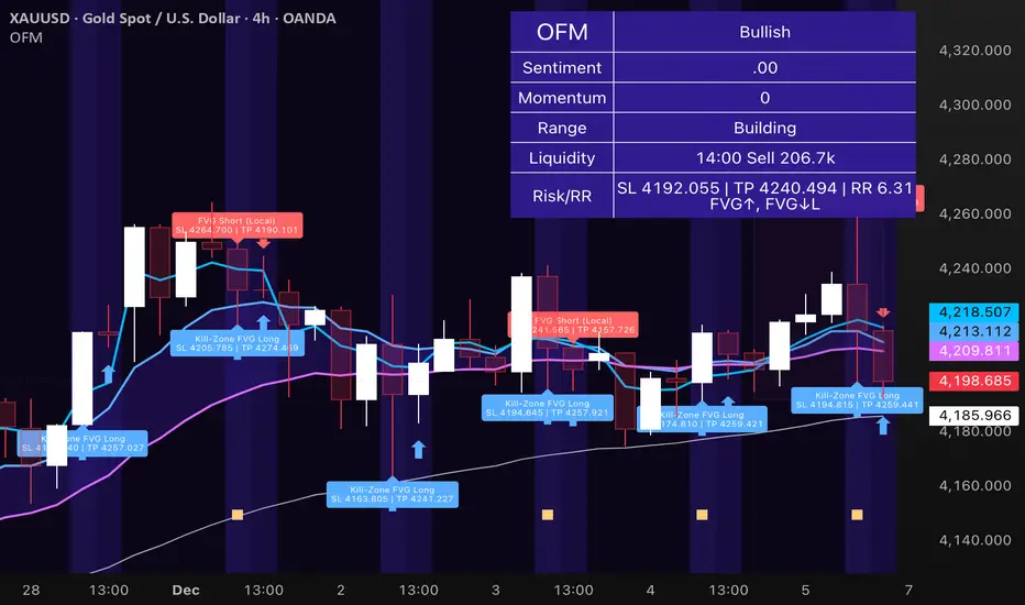
FCPO MASTER v6 – Sideway + Breakout + OB + FVG (TUPLE SAFE)TL;DR cepat
1. Gunakan M5 untuk entry & OB/FVG confirmation.
2. Gunakan M15 untuk confirm trend/false breakout.
3. Gunakan H1 untuk bias arah (overall market).
4. Entry hanya bila signal + OB/FVG/candle rejection (script buatkan).
5. SL 5–8 tick, TP 10–25 tick ikut setup (sideway vs breakout).
6. Follow checklist setiap trade — jangan lompat.
________________________________________
Setup awal (1–2 min)
1. Pasang script FCPO Sideway MASTER – OB + Imbalance + Confirmation di TradingView.
2. Timeframes: buka M5, M15, H1 (susun 3 chart atau 1 chart multi-timeframe).
3. Input default: ATR14, Breakout Buffer 5 tick, RangeLen 20, ADX14, TP12, SL8. (Kau boleh tweak nanti).
4. Aktifkan alerts pada BUY Confirm / SELL Confirm / Sideway Buy / Sideway Sell.
________________________________________
Step-by-step trading process
1) Mulakan dengan H1 — tentukan bias HTF
• Lihat H1 untuk jawapan: Trend Up / Down / Sideway.
• Rule ringkas:
o ADX H1 > 20 + price above H1 EMA → bias Bull
o ADX H1 > 20 + price below H1 EMA → bias Bear
o ADX H1 < 20 → market HTF sideway (no strong bias)
Kenapa: H1 bagi kau idea “kalau breakout pada M5, patut follow atau tolak”.
________________________________________
2) Pergi ke M15 — confirm trend & valid breakout
• M15 kena setuju dengan idea breakout.
o Untuk strong breakout: M15 kena tunjuk candle close di atas/bawah range + volume naik.
o Kalau M5 breakout tapi M15 tak setuju (M15 masih sideway) → treat as fakeout. Jangan masuk.
________________________________________
3) M5 — cari entry & confirmation (OB/FVG + candle)
• M5 adalah tempat kau buat keputusan masuk.
• Tunggu script keluarkan Sideway Buy/Sell atau Breakout Buy/Sell.
• CONFIRM entry mesti ada sekurang-kurangnya 1 dari:
o Bull/Bear Order Block searah signal (script detect).
o FVG / Imbalance zone dipenuhi & price retest.
o Candle rejection (pinbar / bearish/bullish engulfing) pada zone.
Jika tiada confirmation → no trade.
________________________________________
4) Checklist sebelum tekan Buy/Sell (MUST)
• H1 bias tidak melawan trade (prefer sama arah).
• M15 confirm breakout / trend or neutral.
• Script keluarkan signal (sideway or breakout).
• OB or FVG atau candle rejection ada.
• ATR kenaikan jika breakout (untuk breakout trade).
• Volume spike jika breakout.
• Risk:SL <= 2% akaun (position sizing).
Kalau semua ticked → boleh entry.
________________________________________
5) Setting SL / TP & position sizing
• Sideway (scalp): SL = 5–8 tick, TP = 8–12 tick.
• Breakout (trend): SL = 8–12 tick, TP = 15–25+ tick (trail later).
• Position sizing: Risk per trade 1–2%.
o Lot size = (Account Risk RM × 1 tick value) / (SL ticks × tickValue) — (kalau kau gunakan fixed tick value, adjust ikut lot).
(Script tunjuk SL & TP label — follow itu.)
________________________________________
6) Entry types
• A. Sideway Reversal (M5)
o Signal: Sideway Buy / Sideway Sell
o Confirm: OB/FVG or rejection candle at range bottom/top
o Trade: scalp target 8–12 tick, tight SL 5–8 tick
• B. Breakout (M5 entry, M15 confirm)
o Signal: Breakout Buy/Sell (Strong)
o Confirm: ATR expanding + volume spike + M15 alignment
o Trade: trend follow, TP 15–25 tick, trailing stop active
• C. Retest Entry
o Breakout happens, price returns to retest range / OB / FVG → wait for rejection candle then enter. Safer.
________________________________________
7) Trailing & exit rules
• Jika useTrail = true script plots trailing stop (ATR × multiplier).
• Exit rules:
1. Hit TP → close.
2. Hit SL → close.
3. If trailing stop hit → close.
4. If opposing confirmed signal muncul (e.g., SELL confirm while long) → consider close early.
5. If H1 bias flips strongly vs trade → tighten stop or close.
________________________________________
8) Multiple signals & scaling
• Never add to losing position (no averaging down).
• If want scale-in on confirmed trend: add 1 partial size after price moves +10–12 tick in favor and shows continuation candle + no bearish OB/FVG.
• Keep aggregated risk within your max (2–3%).
________________________________________
9) Example trade walkthrough (concrete)
• RangeHigh = 4065, RangeLow = 4035 (contoh).
• Market sideway M5.
Case A — Sideway Sell:
1. Price touches 4064–4065, script shows sidewaySell.
2. Lihat OB: ada bear OB zone di 4062–4066 → confirm.
3. Candle rejection (bearish pinbar) muncul → enter SELL M5.
4. Set SL = 5 tick above rangeHigh = 4070, TP = 10 tick → 4055.
5. Trail jika price turun > 8 tick: aktifkan trailing.
6. Close at TP or trail/SL.
Case B — Breakout Buy:
1. Price closes above 4065 + 5 tick buffer = 4070 on M5. Script shows trueBreakUp.
2. M15 shows candle close above M15 resistance + volume spike → confirm.
3. Enter BUY, SL = 8 tick below entry, TP initial 20 tick, trail with ATR×1.5.
4. Move stop to breakeven after +10 tick, scale out half at +12 tick, leave rest to trail.
________________________________________
10) Journal & review
• Semua trade: record entry time, TF, reason (which confirmations), SL/TP, result, lesson.
• Weekly review: check which confirmation worked best (OB vs FVG vs candle) and tweak settings.
________________________________________
11) Tweaks / optimisations cepat
• Jika terlalu banyak false sideway signals → kurangkan touchDist ke 2 tick.
• Kalau fakeout breakout banyak → tambah tickBuf ke 6–8.
• Nak lebih konservatif → cuma trade breakout yang juga setuju M15.
________________________________________
12) Alerts & execution (practical)
• Pasang alert pada BUY Confirm / SELL Confirm (script).
• Kalau kau guna broker yang support one-click order, siap sediakan template order (SL/TP default).
• Kalau manual, bila alert masuk: buka M5, cepat confirm OB/FVG & candle rejection → entry.
________________________________________
Quick reference table (handy)
• TF utama entry: M5
• Confirm mid-TF: M15
• Bias HTF: H1
• Sideway SL/TP: SL 5–8, TP 8–12
• Breakout SL/TP: SL 8–12, TP 15–25+
• Mandatory confirmation: (Script signal) + (OB or FVG or candle)

Linear Trajectory & Volume StructureThe Linear Trajectory & Volume Structure indicator is a comprehensive trend-following system designed to identify market direction, volatility-adjusted channels, and high-probability entry points. Unlike standard Moving Averages, this tool utilizes Linear Regression logic to calculate the "best fit" trajectory of price, encased within volatility bands (ATR) to filter out market noise.
It integrates three core analytical components into a single interface:
Trend Engine: A Linear Regression Curve to determine the mean trajectory.
Volume Verification: Filters signals to ensure price movement is backed by market participation.
Market Structure: Identifies previous high-volume supply and demand zones for support and resistance analysis.
2. Core Components and Logic
The Trajectory Engine
The backbone of the system is a Linear Regression calculation. This statistical method fits a straight line through recent price data points to determine the current slope and direction.
The Baseline: Represents the "fair value" or mean trajectory of the asset.
The Cloud: Calculated using Average True Range (ATR). It expands during high volatility and contracts during consolidation.
Trend Definition:
Bullish: Price breaks above the Upper Deviation Band.
Bearish: Price breaks below the Lower Deviation Band.
Neutral/Chop: Price remains inside the cloud.
Smart Volume Filter
The indicator includes a toggleable volume filter. When enabled, the script calculates a Simple Moving Average (SMA) of the volume.
High Volume: Current volume is greater than the Volume SMA.
Signal Validation: Reversal signals and structure zones are only generated if High Volume is present, reducing the likelihood of trading false breakouts on low liquidity.
Volume Structure (Smart Liquidity)
The script automatically plots Support (Demand) and Resistance (Supply) boxes based on pivot points.
Creation: A box is drawn only if a pivot high or low is formed with High Volume (if the volume filter is active).
Mitigation: The boxes extend to the right. If price breaks through a zone, the box turns gray to indicate the level has been breached.
3. Signal Guide
Trend Reversals (Buy/Sell Labels)
These are the primary signals indicating a potential change in the macro trend.
BUY Signal: Appears when price closes above the upper volatility band after previously being in a downtrend.
SELL Signal: Appears when price closes below the lower volatility band after previously being in an uptrend.
Pullbacks (Small Circles)
These are continuation signals, useful for adding to positions or entering an existing trend.
Long Pullback: The trend is Bullish, but price dips momentarily below the baseline (into the "discount" area) and closes back above it.
Short Pullback: The trend is Bearish, but price rallies momentarily above the baseline (into the "premium" area) and closes back below it.
4. Configuration and Settings
Trend Engine Settings
Trajectory Length: The lookback period for the Linear Regression. This is the most critical setting for tuning sensitivity.
Channel Multiplier: Controls the width of the cloud.
1.0: Aggressive. Results in narrower bands and earlier signals, but more false positives.
1.5: Balanced (Default).
2.0+: Conservative. Creates a wide channel, filtering out significant noise but delaying entry signals.
Signal Logic
Show Trend Reversals: Toggles the main Buy/Sell labels.
Show Pullbacks: Toggles the re-entry circle signals.
Smart Volume Filter: If checked, signals require above-average volume. Unchecking this yields more signals but removes the volume confirmation requirement.
Volume Structure
Show Smart Liquidity: Toggles the Support/Resistance boxes.
Structure Lookback: Defines how many bars constitute a pivot. Higher numbers identify only major market structures.
Max Active Zones: Limits the number of boxes on the chart to prevent clutter.
5. Timeframe Optimization Guide
To maximize the effectiveness of the Linear Trajectory, you must adjust the Trajectory Length input based on your trading style and timeframe.
Scalping (1-Minute to 5-Minute Charts)
Recommended Length: 20 to 30
Multiplier: 1.2 to 1.5
Logic: Fast-moving markets require a shorter lookback to react quickly to micro-trend changes.
Day Trading (15-Minute to 1-Hour Charts)
Recommended Length: 55 (Default)
Multiplier: 1.5
Logic: A balance between responsiveness and noise filtering. The default setting of 55 is standard for identifying intraday sessions.
Swing Trading (4-Hour to Daily Charts)
Recommended Length: 89 to 100
Multiplier: 1.8 to 2.0
Logic: Swing trading requires filtering out intraday noise. A longer length ensures you stay in the trade during minor retracements.
6. Dashboard (HUD) Interpretation
The Head-Up Display (HUD) provides a summary of the current market state without needing to analyze the chart visually.
Bias: Displays the current trend direction (BULLISH or BEARISH).
Momentum:
ACCELERATING: Price is moving away from the baseline (strong trend).
WEAKENING: Price is compressing toward the baseline (potential consolidation or reversal).
Volume: Indicates if the current candle's volume is HIGH or LOW relative to the average.
Disclaimer
*Trading cryptocurrencies, stocks, forex, and other financial instruments involves a high level of risk and may not be suitable for all investors. This indicator is a technical analysis tool provided for educational and informational purposes only. It does not constitute financial advice, investment recommendations, or a guarantee of profit. Past performance of any trading system or methodology is not necessarily indicative of future results.

ChronoFlow## ChronoFlow Sentinel
ChronoFlow Sentinel is a regime console that blends normalized fast/mid/slow regression slopes, phases them against a dual-speed EMA spread, and grades alignment so you instantly know whether the time stack is trending, rotating, or fighting itself.
HOW IT WORKS
Multi-Timeframe Slopes – Linear regression slopes are fetched via request.security() for your chosen fast, mid, and slow frames.
Normalized Weighting – User weights are rescaled so the composite chrono score is always on a consistent scale, regardless of configuration.
Phase Differential – The indicator subtracts a slow EMA from a fast EMA to detect whether price impulse confirms the slope mix.
Alignment Score – Signs of the three slopes are compared to compute a 0-1 alignment metric; backgrounds and alerts use this to signal confidence vs. chop.
Diagnostics Console – A bottom-right table streams each slope, the blended score, and which timeframe currently dominates.
HOW TO USE IT
Trend Qualification : Only push multi-contract positions when chrono score is positive, phase is positive, and alignment stays above your alert threshold (default 0.66).
Chop Defense : When alignment dips and conflict markers appear, immediately switch into mean-reversion tactics or sit flat.
Swing + Intraday Bridge : Pair ChronoFlow with other structure tools; require both aligned backgrounds and price confirmation before committing to swing entries.
CRYPTOCAP:SOL | CRYPTOCAP:XRP side by side view with ChronoFlow
VISUAL FEATURES
Optional flow curves: Enable Plot Raw Flows to audit each timeframe's slope when troubleshooting a signal.
Background intensity: Opacity auto-adjusts with alignment, so weak trends look faded while strong regimes glow vividly.
Signal/Conflict toggles: Long/short and chop markers are opt-in, keeping the panel pristine until you need annotations.
Conflict alerts: Built-in alert condition fires whenever alignment falls below your threshold, warning execution layers to scale down risk.
PARAMETERS
Fast Frame (default: 30): Fast timeframe for regression slope calculation.
Mid Frame (default: 120): Mid timeframe for regression slope calculation.
Slow Frame (default: D): Slow timeframe for regression slope calculation.
Fast Regression (default: 21): Regression length for fast timeframe.
Mid Regression (default: 34): Regression length for mid timeframe.
Slow Regression (default: 55): Regression length for slow timeframe.
Phase Length (default: 13): EMA period for phase differential calculation.
Fast Weight (default: 0.45): Influence of the fast timeframe in the composite score.
Mid Weight (default: 0.35): Influence of the mid timeframe in the composite score.
Slow Weight (default: 0.20): Influence of the slow timeframe in the composite score.
Plot Raw Flows (default: disabled): Enable to audit each timeframe's slope when troubleshooting.
Show Signal Labels (default: disabled): Toggle long/short signal markers.
Show Conflict Labels (default: disabled): Toggle conflict/chop markers.
Conflict Alert Level (default: 0.66): Set the alignment threshold that should trigger reduced size or flat positioning.
ALERTS
The indicator includes three alert conditions:
ChronoFlow Bullish: Detected a bullish regime shift
ChronoFlow Bearish: Detected a bearish regime shift
ChronoFlow Conflict: Flagged a low-alignment regime
LIMITATIONS
This indicator requires access to multiple timeframes via request.security() , which may consume additional resources. The alignment score is a simplified metric—real market conditions are more complex than a 0-1 scale can capture. The phase differential calculation assumes EMA spreads are meaningful proxies for momentum, which may not hold in all market regimes. Users should test parameter combinations on their specific instruments and timeframes, as default values are optimized for typical index futures trading.
---

Volumetric Inverse Fair Value Gap (IFVG) [Kodexius]The Volumetric Inverse Fair Value Gap (IFVG) indicator detects and visualizes inverse fair value gaps (IFVGs) zones where previous inefficiencies in price (fair value gaps) are later invalidated or “inverted.”
Unlike traditional FVG indicators, this tool integrates volume-based analysis to quantify the bullish, bearish, and overall strength of each inversion. It visually represents these metrics within a dynamically updating box on the chart, giving traders deeper insight into market reactions when liquidity imbalances are filled and reversed.
Features
Inverse fair value gap detection
The script identifies bullish and bearish fair value gaps, stores them as pending zones, and turns them into inverse fair value gaps when price trades back through the gap in the opposite direction. Each valid inversion becomes an active IFVG zone on the chart.
Sensitivity control with ATR filter and strict mode
A minimum gap size based on ATR is used to filter out small and noisy gaps. Strict mode can be enabled so that any wick contact between the relevant candles prevents the gap from being accepted as a fair value gap. This lets you decide how clean and selective the zones should be.
Show Last N Boxes control
The indicator can keep only the most recent N IFVG zones visible. Older zones are removed from the chart once the number of active objects exceeds the user setting. This prevents clutter on higher timeframes or long histories and keeps attention on the most relevant recent zones.
Ghost box for the original gap
When the ghost option is enabled, the script draws a faint box that marks the original fair value gap from which the inverse zone came. This makes it easy to see where the initial imbalance appeared and how price later inverted that area.
Volumetric bull, bear and strength metrics
For each IFVG, the script estimates how much of the bar volume is associated with buying and how much with selling, then computes bull percentage, bear percentage and a strength score that uses a percentile rank of volume. These values are stored with the IFVG object and drive the visualization inside the zone.
Three band visual layout inside each IFVG
Each active IFVG is drawn as a container with three horizontal sections. The top band represents the bull percentage, the middle band the bear percentage and the bottom band the strength metric. The width of each bar reflects its respective value so you can read the structure of the zone at a glance.
Customizable colors and label text
Colors for bull, bear, strength, the empty background area, the ghost box and label text can be adjusted in the inputs. This allows you to match the indicator to different chart themes or highlight specific aspects such as strength or direction.
Automatic invalidation and cleanup
When price clearly closes beyond the IFVG in a way that breaks the logic of that zone, the script marks it as inactive and deletes all boxes and labels linked to it. Only valid and active IFVGs remain on the chart, which keeps the display clean and focused.
Calculations
1. Detecting Fair Value Gaps (FVGs)
A fair value gap is identified when price action leaves an imbalance between candle wicks. Depending on the mode:
Bullish FVG: When low > high
Bearish FVG: When high < low
Optionally, the strict mode ensures wicks do not touch.
The gap’s significance is filtered using the ATR multiplier input to exclude minor noise.
Once detected, FVGs are stored as pending zones until inverted by opposite movement (price crossing through).
bool bull_cond = strict_mode ? (low > high ) : (close > high )
bool bear_cond = strict_mode ? (high < low ) : (close < low )
float gap_size = 0.0
if bull_cond and close > open
gap_size := low - high
if bear_cond and close < open
gap_size := low - high
2. Creating IFVGs (Inversions)
When price later moves through a previous FVG in the opposite direction, an Inverse FVG (IFVG) is created.
For example:
A previous bearish FVG becomes bullish IFVG if price moves upward through it.
A previous bullish FVG becomes bearish IFVG if price moves downward through it.
The IFVG is initialized with structural boundaries (top, bottom) and timestamp metadata to anchor visualization.
if not p.is_bull_gap and close > p.top
inverted := true
to_bull := true
if p.is_bull_gap and close < p.btm
inverted := true
to_bull := false
3. Volume Metrics (Bull, Bear, Strength)
Each IFVG calculates buy and sell volumes from the current bar’s price spread and total volume.
Bull % = proportion of upward (buy) volume
Bear % = proportion of downward (sell) volume
Strength % = normalized percentile rank of total volume
These are obtained through a custom function that estimates directional volume contribution:
calc_metrics(float o, float h, float l, float c, float v) =>
float rng = h - l
float buy_v = 0.0
if rng == 0
buy_v := v * 0.5
else
if c >= o
buy_v := v * ((math.abs(c - o) + (math.min(o, c) - l)) / rng)
else
buy_v := v * ((h - math.max(o, c)) / rng)
float sell_v = v - buy_v
float total = buy_v + sell_v
float p_bull = total > 0 ? buy_v / total : 0
float p_bear = total > 0 ? sell_v / total : 0
float p_str = ta.percentrank(v, 100) / 100.0

Strategy: HMA 50 + Supertrend SniperHMA 50 + Supertrend Confluence Strategy (Trend Following with Noise Filtering)
Description:
Introduction and Concept This strategy is designed to solve a common problem in trend-following trading: Lag vs. False Signals. Standard Moving Averages often lag too much, while price action indicators can generate false signals during choppy markets. This script combines the speed of the Hull Moving Average (HMA) with the volatility-based filtering of the Supertrend indicator to create a robust "Confluence System."
The primary goal of this script is not just to overlay two indicators, but to enforce a strict rule where a trade is only taken when Momentum (HMA) and Volatility Direction (Supertrend) are in perfect agreement.
Why this combination? (The Logic Behind the Mashup)
Hull Moving Average (HMA 50): We use the HMA because it significantly reduces lag compared to SMA or EMA by using weighted calculations. It acts as our primary Trend Direction detector. However, HMA can be too sensitive and "whipsaw" during sideways markets.
Supertrend (ATR-based): We use the Supertrend (Factor 3.0, Period 10) as our Volatility Filter. It uses Average True Range (ATR) to determine the significant trend boundary.
How it Works (Methodology) The strategy uses a boolean logic system to filter out low-quality trades:
Bullish Confluence: The HMA must be rising (Slope > 0) AND the Close Price must be above the Supertrend line (Uptrend).
Bearish Confluence: The HMA must be falling (Slope < 0) AND the Close Price must be below the Supertrend line (Downtrend).
The "Choppy Zone" (Noise Filter): This is a unique feature of this script. If the HMA indicates one direction (e.g., Rising) but the Supertrend indicates the opposite (e.g., Downtrend), the market is considered "Choppy" or indecisive. In this state, the script paints the candles or HMA line Gray and exits all positions (optional setting) to preserve capital.
Visual Guide & Signals To make the script easy to interpret for traders who do not read Pine Script, I have implemented specific visual cues:
Green Cross (+): Indicates a LONG entry signal. Both HMA and Supertrend align bullishly.
Red Cross (X): Indicates a SHORT entry signal. Both HMA and Supertrend align bearishly.
Thick Line (HMA): The main line changes color based on the trend.
Green: Bullish Confluence.
Red: Bearish Confluence.
Gray: Divergence/Choppy (No Trade Zone).
Thin Step Line: This is the Supertrend line, serving as your dynamic Trailing Stop Loss.
Strategy Settings
HMA Length: Default is 50 (Mid-term trend).
ATR Factor/Period: Default is 3.0/10 (Standard for trend catching).
Exit on Choppy: A toggle switch allowing users to decide whether to hold through noise or exit immediately when indicators disagree.
Risk Warning This strategy performs best in trending markets (Forex, Crypto, Indices). Like all trend-following systems, it may experience drawdown during prolonged accumulation/distribution phases. Please backtest with your specific asset before using it with real capital.

Bollinger Bands Delta Matrix Analytics [BDMA] Bollinger Bands Delta Matrix Analytics (BDMA) v7.0
Deep Kinetic Engine – 5x8 Volatility & Delta Decision Matrix
1. Introduction & Concept
Bollinger Bands Delta Matrix Analytics (BDMA) v7.0 is an analytical framework that merges:
- Spatial analysis via Bollinger Bands (%B location),
- with a 4-factor Deep Kinetic Engine based on:
• Total Volume
• Buy Volume
• Sell Volume
• Delta (Buy – Sell) Z-Scores
and converts them into an expanded 5×8 decision matrix that continuously tracks where price is trading and how the underlying orderflow is behaving.
BDMA is not a trading system or strategy. It does not generate entry/exit signals.
Instead, it provides a structured contextual map of volatility, volume, and delta so traders can:
- identify climactic extensions vs. fakeouts,
- distinguish strong initiative moves vs. passive absorption,
- and detect squeezes, traps, and liquidity voids with a unified visual dashboard.
2. Spatial Engine – Bollinger S-States (S1–S5)
The spatial dimension of BDMA comes from classic Bollinger Bands.
Price location is expressed as Percent B (%B) and mapped into 5 spatial states (S-States):
S1 – Hyper Extension (Above Upper Band)
Price has pushed beyond the upper Bollinger Band.
Often associated with parabolic or blow-off behavior, late-stage momentum, and elevated reversal risk.
S2 – Resistance Test (Upper Zone)
Price trades in the upper Bollinger region but remains inside the bands.
Represents a sustained test of resistance, typically within an established or emerging uptrend.
S3 – Neutral Zone (Middle)
Price hovers around the mid-band.
This is the mean reversion gravity field where the market often consolidates or transitions between regimes.
S4 – Support Test (Lower Zone)
Price trades in the lower Bollinger region but inside the bands.
Represents a sustained test of support within range or downtrend structures.
S5 – Hyper Drop (Below Lower Band)
Price extends below the lower Bollinger Band.
Often aligned with panic, forced liquidations, or capitulation-type behavior, with increased snap-back risk.
These 5 S-States define the vertical axis (rows) of the BDMA matrix.
3. Deep Kinetic Engine – 4-Factor Z-Score & D-States (D1–D8)
The Deep Kinetic Engine transforms raw volume and delta into standardized Z-Scores to measure how abnormal current activity is relative to its recent history.
For each bar:
- Raw Buy Volume is estimated from the candle’s position within its range
- Raw Sell Volume is complementary to buy volume
- Raw Delta = Buy Volume – Sell Volume
- Total Volume = Buy Volume + Sell Volume
These 4 series are then normalized using a unified Z-Score lookback to produce:
1. Z_Vol_Total – overall activity and liquidity intensity
2. Z_Vol_Buy – aggression from buyers (attack)
3. Z_Vol_Sell – aggression from sellers (defense or attack)
4. Z_Delta – net victory of one side over the other
Thresholds for Extreme, Significant, and Neutral Z-Score levels are fully configurable, allowing you to tune the sensitivity of the kinetic states.
Using Z_Vol_Total and Z_Delta (plus threshold logic), BDMA assigns one of 8 Deep Kinetic states (D-States):
D1 – Climax Buy
Extreme Total Volume + Extreme Positive Delta → Buying climax or blow-off behavior.
D2 – Strong Buy
High Volume + High Positive Delta → Confirmed bullish initiative activity.
D3 – Weak Buy / Fakeout
Low Volume + High Positive Delta → Bullish delta without commitment, low-liquidity breakout risk.
D4 – Absorption / Conflict
High Volume + Neutral Delta → Aggressive two-way trade, strong absorption, war zone behavior.
D5 – Neutral
Low Volume + Neutral Delta → Low-energy environment with low conviction.
D6 – Weak Sell / Fakeout
Low Volume + High Negative Delta → Bearish delta without commitment, low-liquidity breakdown risk.
D7 – Strong Sell
High Volume + High Negative Delta → Confirmed bearish initiative activity.
D8 – Capitulation
Extreme Volume + Extreme Negative Delta → Panic selling or capitulation regime.
These 8 D-States define the horizontal axis (columns) of the BDMA matrix.
4. The 5×8 BDMA Decision Matrix
The core of BDMA is a 5×8 matrix where:
- Rows (1–5) = Spatial S-States (S1…S5)
- Columns (1–8) = Kinetic D-States (D1…D8)
Each of the 40 possible combinations (SxDy) is pre-computed and mapped to:
- a Status or Regime Title (for example: Climax Breakout, Bear Trap Spring, Capitulation Breakdown),
- a Bias (Climactic Bull, Neutral, Strong Bear, Conflict or Reversal Risk, and similar labels),
- and a Strategic Signal or Consideration (for example: High reversal risk, Wait for confirmation, Low probability zone – avoid).
Internally, BDMA resolves all 40 regimes so the current state can be displayed on the dashboard without performance overhead.
5. Key Regime Families (How to Read the Matrix)
5.1. Breakouts and Breakdowns
Climax Breakout (Top-side)
Spatial S1 with Kinetic D1 or D2
Bias: Explosive or Extreme Bull
Signal:
- Strong or climactic upside extension with abnormal bullish orderflow.
- Trend continuation is possible, but reversal risk is extremely high after blow-off phases.
Low-Conviction Breakout (Fakeout Risk)
S1 with D3 (Weak Buy, low liquidity)
Bias: Weak Bull – Caution
Signal:
- Breakout not supported by volume.
- Elevated risk of failed auction or bull trap.
Capitulation Breakdown (Bottom-side)
Spatial S5 with Kinetic D8
Bias: Climactic Bear (panic)
Signal:
- Capitulation-type selling or forced liquidations.
- Trend can still proceed, but snap-back or violent short-covering risk is high.
Initiative Breakdown vs. Weak Breakdown
- Strong, high-volume breakdown typically corresponds to D7 (Strong Sell).
- Low-volume breakdown often corresponds to D6 (Weak Sell or Fakeout) with potential for failure.
5.2. Absorption, Traps and Springs
Absorption at Resistance (Top-side conflict)
S1 or S2 with D4 (Absorption or Conflict)
Bias: Conflict – Extreme Tension
Signal:
- Heavy two-way trade near resistance.
- Potential distribution or reversal if sellers begin to dominate.
Bull Trap or Failed Auction
Typically S1 with D6 (Weak Sell breakdown behavior after a top-side attempt)
Indicates a breakout attempt that fails and reverses, often after poor liquidity structure.
Absorption at Support and Bear Trap (Spring)
S4 or S5 with D4 or D3
Bias: Conflict or Weak Bear – Reversal Risk
Signal:
- Aggressive buying into lows (spring or shakeout behavior).
- Potential bear trap if price reclaims lost territory.
5.3. Trend Phases
Strong Uptrend Phases
Typically seen when S2–S3 combine with strong bullish kinetic behavior.
Bias: Strong or Extreme Bull
Signal:
- Pullbacks into S3 or S4 with supportive kinetic states often act as trend continuation zones.
Strong Downtrend Phases
Typically seen when S3–S4 combine with strong bearish kinetic behavior.
Bias: Strong or Extreme Bear
Signal:
- Rallies into resistance with strong bearish kinetic backing may act as continuation sell zones.
5.4. Neutral, Exhaustion and Squeeze
Exhaustion or Liquidity Void
S1 or S5 with D5 (Neutral kinetics)
Bias: Neutral or Exhaustion
Signal:
- Spatial extremes without kinetic confirmation.
- Often marks the end of a move, with poor follow-through.
Choppy, Low-Activity Range
S3 with D5
Bias: Neutral
Signal:
- Low volume, low conviction market.
- Typically a low-probability environment where standing aside can be logical.
Squeeze or High-Tension Zone
S3 with D4 or tightly clustered kinetic values
Bias: Conflict or High Tension
Signal:
- Hidden battle inside a volatility contraction.
- Often precedes large directionally-biased moves.
6. Dashboard Layout & Reading Guide
When Show Dashboard is enabled, BDMA displays:
1. Title and Status Line
Name of the current regime (for example: Climax Breakout, Bear Trap Spring, Mean Reversion).
2. Bias Line
Plain-language summary of directional context such as Climactic Bull, Strong Bear, Neutral, or Conflict and Reversal Risk.
3. Signal or Strategic Notes
Concise guidance focused on risk and context, not entries. For example:
- High reversal risk – aggressive traders only
- Wait for confirmation (break or rejection)
- Low probability zone – avoid taking new positions
4. Kinetic Profile (4-Factor Z-Score)
Shows the current Z-Scores for Total Volume (Activity), Buy Volume (Attack), Sell Volume (Defense), and Delta (Net Result).
5. Matrix Heatmap (5×8)
Visual representation of S-State vs. D-State with color coding:
- Bullish clusters in a green spectrum
- Bearish clusters in a red spectrum
- Conflict or exhaustion zones in yellow, amber, or neutral tones
The dashboard can be repositioned (top right, middle right, or bottom right) and its size can be adjusted (Tiny, Small, Normal, or Large) to fit different layouts.
7. Inputs & Customization
7.1. Core Parameters (Bollinger and Z-Score)
- Bollinger Length and Standard Deviation define the spatial engine.
- Z-Score Lookback (All Factors) defines how many bars are used to normalize volume and delta.
7.2. Deep Kinetic Thresholds
- Extreme Threshold defines what is considered climactic (D1 or D8).
- Significant Threshold distinguishes strong initiative vs. weak or fakeout behavior.
- Neutral Threshold is the band within which delta is treated as neutral.
These thresholds allow you to tune the sensitivity of the kinetic classification to fit different timeframes or instruments.
7.3. Calculation Method (Volume Delta)
Geometry (Approx)
- Fast, non-repainting approach based on candle geometry.
- Suitable for most users and real-time decision-making.
Intrabar (Precise)
- Uses lower-timeframe data for more precise volume delta estimation.
- Intrabar mode can repaint and requires compatible data and plan support on the platform.
- Best used for post-analysis or research, not blind automation.
7.4. Visuals and Interface
- Toggle Bollinger Bands visibility on or off.
- Switch between Dark and Light color themes.
- Configure dashboard visibility, matrix heatmap display, position, and size.
8. Multi-Language Semantic Engine (Asia and Middle East Focus)
BDMA v7.0 includes a fully integrated multi-language layer, targeting a wide geographic user base.
Supported Languages:
English, Türkçe, Русский, 简体中文, हिन्दी, العربية, فارسی, עברית
All dashboard labels, regime titles, bias descriptions, and signal texts are dynamically translated via an internal dictionary, while semantic meaning is kept consistent across languages.
This makes BDMA suitable for multi-language communities, study groups, and educational content across different regions.
However, due to the heavy computational load of the Deep Kinetic Engine and TradingView’s strict Pine Script execution limits, it was not possible to expand support to additional languages. Adding more translation layers would significantly increase memory usage and exceed runtime constraints. For this reason, the current language set represents the maximum optimized configuration achievable without compromising performance or stability.
9. Practical Usage Notes
BDMA is most powerful when used as a contextual overlay on top of market structure (HH, HL, LH, LL), higher-timeframe trend, key levels, and your own execution framework.
Recommended usage:
- Identify the current regime (Status and Bias).
- Check whether price location (S-State) and kinetic behavior (D-State) agree with your trade idea.
- Be especially cautious in climactic and absorption or conflict zones, where volatility and risk can be elevated.
Avoid treating BDMA as an automatic green equals buy, red equals sell tool.
The real edge comes from understanding where you are in the volatility or kinetic spectrum, not from forcing signals out of the matrix.
10. Limitations & Important Warnings
BDMA does not predict the future.
It organizes current and recent data into a structured context.
Volume data quality depends on the underlying symbol, exchange, and broker feed.
Forex, crypto, indices, and stocks may all behave differently.
Intrabar mode can repaint and is sensitive to lower-timeframe data availability and your plan type.
Use it with extra caution and primarily for research.
No indicator can remove the need for clear trading rules, disciplined risk management, and psychological control.
11. Disclaimer
This script is provided strictly for educational and analytical purposes.
It is not a trading system, signal service, financial product, or investment advice.
Nothing in this indicator or its description should be interpreted as a recommendation to buy or sell any asset.
Past behavior of any indicator or market pattern does not guarantee future results.
Trading and investing involve significant risk, including the risk of losing more than your initial capital in leveraged products.
You are solely responsible for your own decisions, risk management, and results.
By using this script, you acknowledge that you understand these risks and agree that the author or authors and publisher or publishers are not liable for any loss or damage arising from its use.
