Supply In Profit Z-ScoreZ-score of BTC Supply in Profit.
Supply in Profit is an On-Chain BTC indicator that shows the percentage of BTC in profit.
In this indicator you can choose to use a Z-Score or not.
Cerca negli script per "btc期权交割时间"

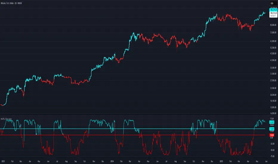
NUPL-Z For Loop🧠 Overview
NUPL-Z For Loop is a trend-following indicator built on Bitcoin’s on-chain Net Unrealized Profit/Loss (NUPL) metric. It uses a Z-scored transformation of NUPL and a custom loop-based scoring system to measure the consistency of directional movement. Rather than identifying tops and bottoms, this tool is designed to track sustained trends and filter out short-term noise, making it ideal for momentum-aligned strategies.
🧩 Key Features
Loop-Based Trend Logic: Assesses trend strength by summing the number of upward vs. downward moves in Z-scored NUPL across a custom lookback.
Z-Score Normalization: Applies long-term statistical normalization to NUPL to emphasize deviation from average behavior over time.
Threshold-Based Regime Shifts: Custom input thresholds define when trend strength is significant enough to trigger long or short signals.
Directional Market State Tracking: Internally tracks bullish, bearish, or neutral conditions to guide trend entries.
BTC-Focused On-Chain Analysis: Tailored specifically for Bitcoin using Market Cap and Realized Cap inputs.
🔍 How It Works
NUPL Calculation: Derived as the percentage of net unrealized profit relative to market cap: (MC - RMC) / MC * 100.
Z-Scoring: NUPL is normalized using a rolling mean and standard deviation over a long window (default 1300 days) to create a smoothed trend signal.
Directional Loop: A custom loop iterates from the start_loop to the end_loop, comparing the current Z-score to past values.
Each instance where NUPL_Z > NUPL_Z adds +1 to the score; otherwise, it subtracts -1.
This cumulative score reflects how consistently NUPL-Z has been trending.
Signal Logic:
Long signal when loop score exceeds long_threshold.
Short signal when score falls below short_threshold.
CD State Engine: Maintains the current trend regime (1 for long, -1 for short), which drives plot coloring and overlays.
🔁 Use Cases & Applications
Momentum Trend Filter: Detects and confirms sustained directional strength in BTC’s profit/loss positioning.
Noise Suppression: Avoids reactive signals from one-off spikes or dips in NUPL by requiring a consistent trend before confirming bias.
Best Suited for BTC: Designed specifically for Bitcoin’s price and on-chain structure, using its unique NUPL dynamics.
✅ Conclusion
NUPL-Z For Loop transforms a traditionally mean-reverting indicator into a trend-following signal engine. By scoring the consistency of movement in normalized NUPL, this tool identifies trend strength rather than reversal potential — providing more reliable context for momentum-aligned trades on Bitcoin.
⚠️ Disclaimer
The content provided by this indicator is for educational and informational purposes only. Nothing herein constitutes financial or investment advice. Trading and investing involve risk, including the potential loss of capital. Always backtest and apply risk management suited to your strategy.
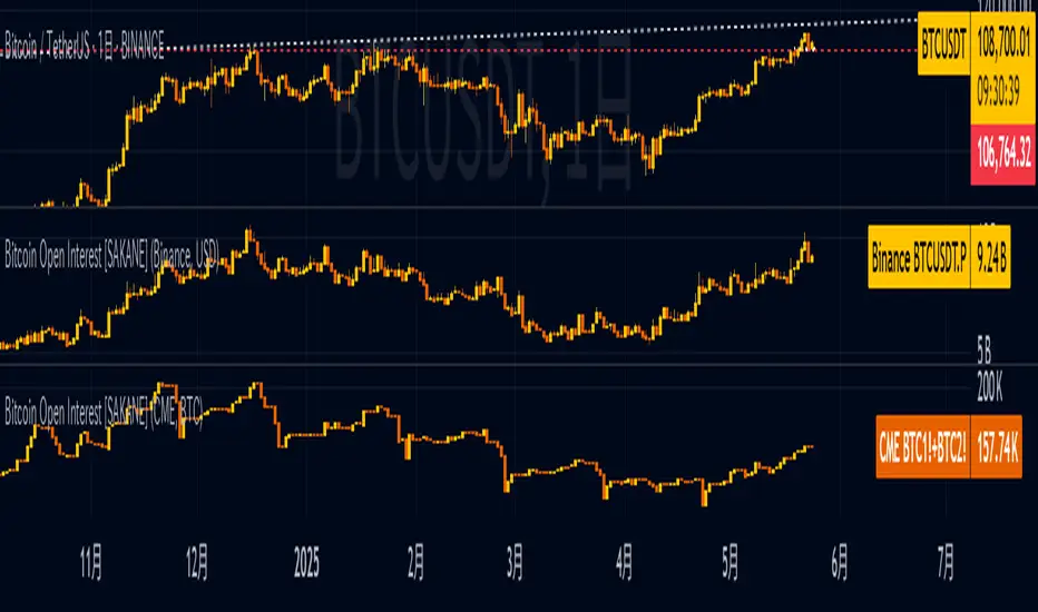
Bitcoin Open Interest [SAKANE]Bitcoin Open Interest
— Unveiling the True Flow of Capital
PurposeVisualize and compare Bitcoin open interest (OI) from CME and Binance, the leading derivatives exchanges, in a single intuitive chart, providing traders with clear insights into crypto market capital dynamics.
Background & MotivationIn the 24/7 crypto market, price movements alone reveal only part of the story. Open interest (OI)—the total outstanding futures contracts—offers critical clues to the market’s next move. Yet, accessing and interpreting OI data is challenging:
CME Constraints: Commitment of Traders (COT) reports are weekly, and standalone BTC1! or BTC2! OI is noisy due to contract rollovers, obscuring true OI changes.
Existing Tool Limitations: Most OI indicators are fixed to either USD or BTC, limiting flexible analysis.
This indicator overcomes these hurdles, enabling seamless comparison of CME and Binance OI to track the market’s “capital center of gravity” in real time.
Key Features
Synthetic CME OI: Combines BTC1! and BTC2! to deliver high-accuracy OI, eliminating rollover noise.
Multi-Timeframe Analysis: Displays daily CME OI as pseudo-candlestick (OHLC) on any timeframe (e.g., 4H), allowing intuitive capital flow tracking across timeframes.
CME/Binance One-Click Toggle: Instantly compare institutional-driven CME and retail-driven Binance OI.
USD/BTC Flexibility: Switch between BTC (real demand) and USD (margin) perspectives for OI analysis.
Robust Design: Concise, global-scope code ensures stability and adaptability to TradingView updates.
Insights & Use Cases
Holistic Market Sentiment: Analyze capital flows by region and exchange for a multidimensional view.
Signal Detection: E.g., a sharp drop in CME OI during a sell-off may signal institutional withdrawal.
Retail Trends: A surge in Binance OI suggests retail-driven inflows.
Event-Driven Insights: E.g., during a hypothetical April 2025 “Trump Tariff Shock,” instantly identify which exchange drives capital shifts.
Unique ValueUnlike price-centric indicators, this tool focuses on capital flow (OI). It’s the only indicator offering one-click multi-timeframe and multi-exchange OI comparison, empowering traders to uncover the market’s “true intent” and gain a strategic edge.
ConclusionBitcoin Open Interest makes the market’s hidden capital movements accessible to all. By capturing market dynamics and pinpointing the “leading forces” during events, it sets a new standard for traders seeking a revolutionary perspective.
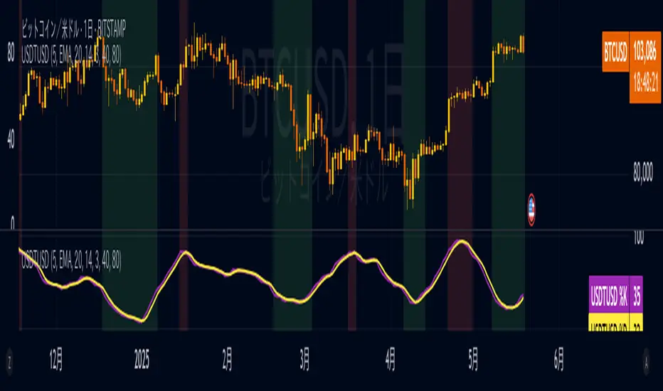
USDTUSD Stochastic RSI [SAKANE]Release Note
■ Overview
The USDTUSD Stochastic RSI indicator visualizes shifts in market sentiment and liquidity by applying the Stochastic RSI to the USDT/USD price pair.
Rather than tracking the price of Bitcoin directly, this tool observes the momentum of USDT, a key intermediary in most crypto transactions, to detect early signals of trend reversals.
■ Background & Motivation
USDT exhibits two distinct characteristics:
Its credibility as a long-term store of value is limited.
Yet, it serves as one of the most liquid assets in the crypto space and is widely used as a trading base pair.
Because most BTC trades involve converting fiat into USDT and vice versa, USDT/USD frequently deviates slightly from its peg to USD.
These deviations—though subtle—often occur just before major shifts in the broader crypto market.
This indicator is designed to detect such moments of structural imbalance by applying momentum analysis to USDT itself.
■ Feature Highlights
Calculates RSI and Stochastic RSI on the USDT/USD closing price
Supports customizable smoothing via SMA or EMA
Background shading dynamically visualizes overheated or cooled market states (thresholds are adjustable)
Displayed in a separate pane, keeping it visually distinct from the price chart
■ Usage Insights
This indicator is based on an observable pattern:
When the Stochastic RSI bottoms out, Bitcoin tends to form a price bottom shortly afterward
Conversely, when the indicator peaks, Bitcoin tends to top out with a slight delay
Since USDT acts as a gateway for capital in and out of the market, changes in its momentum often foreshadow turning points in BTC.
This allows traders to anticipate shifts in sentiment rather than merely reacting to them.
■ Unique Value Proposition
Unlike conventional price-based indicators, this tool offers a structural perspective.
It focuses on USDT as a mechanism of liquidity flow, making it possible to detect the "hidden rhythm" of the crypto market.
In that sense, this is not just a technical tool, but an entry point into market microstructure analysis—allowing users to read the market’s intentions rather than just its movements.
■ Practical Tips
Look for reversals in momentum as potential BTC entry or exit points.
Overlay this indicator with the BTC chart to compare timing and divergence.
Combine with other tools such as on-chain data or macro indicators for comprehensive analysis.
■ Final Thoughts
USDTUSD Stochastic RSI is designed with the belief that the most important market signals often come from what drives the price, not the price itself.
By tuning into the “heartbeat” of capital flow, this indicator sheds light on market dynamics that would otherwise remain unseen.
We hope it proves useful in your trading and research.
MVRV | Lyro RS📊 MVRV | Lyro RS is a powerful on-chain valuation tool designed to assess the relative market positioning of Bitcoin (BTC) or Ethereum (ETH) based on the Market Value to Realized Value (MVRV) ratio. It highlights potential undervaluation or overvaluation zones, helping traders and investors anticipate cyclical tops and bottoms.
✨ Key Features :
🔁 Dual Asset Support: Analyze either BTC or ETH with a single toggle.
📐 Dynamic MVRV Thresholds: Automatically calculates median-based bands at 50%, 64%, 125%, and 170%.
📊 Median Calculation: Period-based median MVRV for long-term trend context.
💡 Optional Smoothing: Use SMA to smooth MVRV for cleaner analysis.
🎯 Visual Threshold Alerts: Background and bar colors change based on MVRV position relative to thresholds.
⚠️ Built-in Alerts: Get notified when MVRV enters under- or overvalued territory.
📈 How It Works :
💰 MVRV Calculation: Uses data from IntoTheBlock and CoinMetrics to obtain real-time MVRV values.
🧠 Threshold Bands: Median MVRV is used as a baseline. Ratios like 50%, 64%, 125%, and 170% signal various levels of market extremes.
🎨 Visual Zones: Green zones for undervaluation and red zones for overvaluation, providing intuitive visual cues.
🛠️ Custom Highlights: Toggle individual threshold zones on/off for a cleaner view.
⚙️ Customization Options :
🔄 Switch between BTC or ETH for analysis.
📏 Adjust period length for median MVRV calculation.
🔧 Enable/disable threshold visibility (50%, 64%, 125%, 170%).
📉 Toggle smoothing to reduce noise in volatile markets.
📌 Use Cases :
🟢 Identify undervalued zones for long-term entry opportunities.
🔴 Spot potential overvaluation zones that may precede corrections.
🧭 Use in confluence with price action or macro indicators for better timing.
⚠️ Disclaimer :
This indicator is for educational purposes only. It should not be used in isolation for making trading or investment decisions. Always combine with price action, fundamentals, and proper risk management.

Crypto Fear & Greed Score [Underblock]Crypto Fear & Greed Score - Methodology & Functioning
Introduction
The Crypto Fear & Greed Score is a comprehensive indicator designed to assess market sentiment by detecting extreme conditions of panic (fear) and euphoria (greed). By combining multiple technical factors, it helps traders identify potential buying and selling opportunities based on the emotional state of the market.
This indicator is highly customizable, allowing users to adjust weight parameters for RSI, volatility, Bitcoin dominance, and trading volume, making it adaptable to different market conditions.
Key Components
The indicator consists of two primary sub-scores:
Fear Score (Panic) - Measures the intensity of fear in the market.
Greed Score (Euphoria) - Measures the level of overconfidence and excessive optimism.
The difference between these two values results in the Net Score, which indicates the dominant market sentiment at any given time.
1. Relative Strength Index (RSI)
The indicator utilizes multiple RSI timeframes to measure momentum and overbought/oversold conditions:
RSI 1D (Daily) - Captures medium-term sentiment shifts.
RSI 4H (4-hour) - Identifies short-term market movements.
RSI 1W (Weekly) - Helps detect long-term overbought/oversold conditions.
2. Volatility Analysis
High volatility is often associated with fear and panic-driven selling.
Low volatility in bullish markets may indicate complacency and overconfidence.
3. Bitcoin Dominance (BTC.D)
Bitcoin dominance provides insights into capital flow between Bitcoin and altcoins:
Rising BTC dominance suggests fear as investors move into BTC for safety.
Declining BTC dominance indicates increased risk appetite and potential market euphoria.
4. Buying and Selling Volume
The indicator analyzes both buying and selling volume, ensuring a clearer confirmation of market sentiment.
High buying volume in uptrends reinforces bullish momentum.
Spikes in selling volume indicate panic and possible market bottoms.
Calculation Methodology
The indicator allows users to adjust weight parameters for each component, making it adaptable to different trading strategies. The formulas are structured as follows:
Fear Score (Panic Calculation)
Fear Score = (1 - RSI_1D) * W_RSI1D + (1 - RSI_4H) * W_RSI4H + (1 - Dominance) * W_Dominance + Volatility * W_Volatility + Sell Volume * W_SellVolume
Greed Score (Euphoria Calculation)
Greed Score = RSI_1D * W_RSI1D + RSI_4H * W_RSI4H + Dominance * W_Dominance + (1 - Volatility) * W_Volatility + Buy Volume * W_BuyVolume
Net Fear & Greed Score
Net Score = (Greed Score - Fear Score) * 100
Interpretation:
Above 70: Extreme greed -> possible overbought conditions.
Below -70: Extreme fear -> potential buying opportunity.
Near 0: Neutral market sentiment.
Trend Reversal Detection
The indicator includes two moving averages for enhanced trend detection:
Short-term SMA (50-periods) - Reacts quicklier to changes in sentiment.
Long-term SMA (200-periods) - Captures broader trend reversals.
How Crossovers Work:
Short SMA crossing above Long SMA -> Potential bullish reversal.
Short SMA crossing below Long SMA -> Possible bearish trend shift.
Alerts for SMA crossovers help traders act on momentum shifts in real-time.
Customization and Visualization
The Net Score dynamically changes color: green for greed, red for fear.
Users can adjust weightings directly from settings, avoiding manual script modifications.
Reference levels at 70 and -70 provide clarity on extreme market conditions.
Conclusion
The Crypto Fear & Greed Score provides a powerful and objective measure of market sentiment, helping traders navigate extreme conditions effectively.
🟢 If the Net Score is below -70, panic may present a buying opportunity.
🔴 If the Net Score is above 70, excessive euphoria may indicate a selling opportunity.
⚖️ Neutral values suggest a balanced market sentiment.
By customizing weight parameters and utilizing trend reversal alerts, traders can gain a deeper insight into market psychology and make more informed trading decisions. 🚀

Delta VolDelta Volume BTC - Multi Pair
Description The Delta Volume BTC - Multi Pair indicator visualizes the balance between buying and selling volume across multiple Bitcoin exchanges. By analyzing price action within each bar, it provides insight into underlying market pressure that traditional volume indicators miss. This indicator allows traders to:
Compare volume flow across Coinbase, Binance, and Binance Perpetual markets
Identify divergences between exchanges that may signal market shifts
Detect accumulation or distribution patterns through volume imbalances
View exchanges individually or in aggregate for comprehensive analysis
Calculation Methods The indicator offers three volume delta calculation methods:
VWAP Based (default):
price_range = high - low
buy_percent = (close - low) / price_range
sell_percent = (high - close) / price_range
delta = volume * (buy_percent - sell_percent)
This method distributes volume based on where price closed within the bar's range, providing a nuanced view of buying/selling pressure.
Tick Based :
delta = volume * sign(hlc3 - previous_hlc3)
This approach assigns volume based on the direction of typical price movement between bars, capturing momentum between periods.
Simple :
delta = close > open ? volume : close < open ? -volume : 0
A straightforward method that assigns positive volume to up bars and negative volume to down bars.
When Aggregate Mode is enabled, the indicator sums the volume deltas from all selected exchanges:
aggregate_delta = coinbase_delta + binance_delta + binance_perp_delta
Features
Multi-Exchange Support : Track volume delta across Coinbase, Binance, and Binance Perpetual futures
Advanced Calculation Methods : Choose between VWAP-based, tick-based, or simple volume delta algorithms
Flexible Display Options : Visualize as histogram, columns, area, or line charts
Customizable Colors : Distinct color schemes for each exchange and direction
Smoothing Options : Apply EMA, SMA, or WMA to reduce noise
Aggregate Mode : Combine all exchanges to see total market flow
How to Use
Individual Exchange Analysis : Uncheck "Aggregate Mode" to see each exchange separately, revealing where smart money may be positioning
Divergence Detection : Watch for one exchange showing buying while others show selling
Volume Trend Confirmation : Strong price moves should be accompanied by strong delta in the same direction
Liquidity Analysis : Compare spot vs futures volume delta to identify market sentiment shifts
The Delta Volume BTC - Multi Pair indicator helps identify the "hidden" buying and selling pressure that may not be apparent from price action alone, giving you an edge in understanding market dynamics across the Bitcoin ecosystem.

SL Hunting Detector📌 Step 1: Identify Liquidity Zones
The script plots high-liquidity zones (red) and low-liquidity zones (green).
These are areas where big players target stop-losses before reversing the price.
Example:
If price is near a red liquidity zone, expect a potential stop-loss hunt & reversal downward.
If price is near a green liquidity zone, expect a potential stop-loss hunt & reversal upward.
📌 Step 2: Watch for Stop-Loss Hunts (Fakeouts)
The indicator marks stop-loss hunts with red (bearish) or green (bullish) arrows.
When do stop-loss hunts occur?
✅ A long wick below support (with high volume) = Stop hunt before reversal upward.
✅ A long wick above resistance (with high volume) = Stop hunt before reversal downward.
Confirmation:
Volume must spike (volume > 1.5x the average volume).
ATR-based wicks must be longer than usual (showing a stop-hunt trap).
📌 Step 3: Enter a Trade After a Stop-Hunt
🔹 Bullish Trade (Buying a Dip)
If a green arrow appears (stop-hunt below support):
✅ Enter a long (buy) trade at or just above the wick’s recovery level.
✅ Stop-loss: Below the wick’s low (avoid getting hunted again).
✅ Take-profit: Next resistance level or mid-range of the liquidity zone.
🔹 Bearish Trade (Shorting a Fakeout)
If a red arrow appears (stop-hunt above resistance):
✅ Enter a short (sell) trade at or just below the wick’s rejection level.
✅ Stop-loss: Above the wick’s high (avoid getting stopped out).
✅ Take-profit: Next support level or mid-range of the liquidity zone.
📌 Step 4: Set Alerts & Automate
✅ The indicator triggers alerts when a stop-hunt is detected.
✅ You can set TradingView to notify you instantly when:
A bullish stop-hunt occurs → Look for long entry.
A bearish stop-hunt occurs → Look for short entry.
📌 Example Trade Setup
Example (BTC Long Trade on Stop-Hunt)
BTC is near $40,000 support (green liquidity zone).
A long wick drops to $39,800 with a green arrow (bullish stop-hunt signal).
Volume spikes, and price recovers quickly back above $40,000.
Trade entry: Buy at $40,050.
Stop-loss: Below wick ($39,700).
Take-profit: $41,500 (next resistance).
Result: BTC pumps, stop-loss remains safe, and trade profits.
🔥 Final Tips
Always wait for confirmation (don’t enter blindly on signals).
Use higher timeframes (15m, 1H, 4H) for better accuracy.
Combine with Order Flow tools (like Bookmap) to see real liquidity zones.
🚀 Now try it on TradingView! Let me know if you need adjustments. 📈🔥

MATA GOLD RATIOMata Gold Instrument: User Guide
The Instrument to Gold Oscillator is a technical analysis tool that normalizes the ratio of an instrument's price (e.g., BTC/USD) to the price of gold (XAU/USD) into a 0-100 scale. This provides a clear and intuitive way to evaluate the relative performance of an instrument compared to gold over a specified period.
---
How It Works
1. Calculation of the Ratio:
The ratio is calculated as:
\text{Ratio} = \frac{\text{Instrument Price}}{\text{Gold Price}}
2. Normalization:
The ratio is normalized using the highest and lowest values over a user-defined period (length), typically 14 periods:
\text{Normalized Ratio} = \frac{\text{Ratio} - \text{Min(Ratio)}}{\text{Max(Ratio)} - \text{Min(Ratio)}} \times 100
3. Overbought/Oversold Levels:
Above 80: The instrument is relatively expensive compared to gold (overbought).
Below 20: The instrument is relatively cheap compared to gold (oversold).
---
How to Use the Oscillator
1. Identify Overbought and Oversold Levels:
If the oscillator rises above 80, the instrument may be overvalued relative to gold. This could signal a potential reversal or correction.
If the oscillator falls below 20, the instrument may be undervalued relative to gold. This could signal a buying opportunity.
2. Track Trends:
Rising oscillator values indicate the instrument is gaining value relative to gold.
Falling oscillator values indicate the instrument is losing value relative to gold.
3. Crossing the Midline (50):
When the oscillator crosses above 50, the instrument's value is gaining strength relative to gold.
When it crosses below 50, the instrument is weakening relative to gold.
4. Combine with Other Indicators:
Use this oscillator alongside other technical indicators (e.g., RSI, MACD, STOCH) for more robust decision-making.
Confirm signals from the oscillator with price action or volume analysis.
---
Example Scenarios
1. Trading Cryptocurrencies Against Gold:
If BTC/USD's oscillator value is above 80, Bitcoin may be overvalued relative to gold. Consider reducing exposure or looking for short opportunities.
If BTC/USD's oscillator value is below 20, Bitcoin may be undervalued relative to gold. This could be a good time to accumulate.
2. Commodities vs. Gold:
Analyze the relative strength of commodities (e.g., oil, silver) against gold using the oscillator to identify periods of overperformance or underperformance.
---
Advantages of the Oscillator
Relative Performance Insight: Tracks the performance of an instrument relative to gold, providing a macro perspective.
Clear Visual Representation: The 0-100 scale makes it easy to identify overbought/oversold conditions and trend shifts.
Customizable Periods: The user-defined length allows flexibility in analyzing short- or long-term trends.
---
Limitations
Dependence on Gold: As the oscillator is based on gold prices, any external shocks to gold (e.g., geopolitical events) can influence its signals.
No Absolute Buy/Sell Signals: The oscillator should not be used in isolation but as part of a broader analysis strategy.
---
By using the Instrument to Gold Oscillator effectively, traders and investors can gain valuable insights into the relative valuation and performance of assets compared to gold, enabling more informed trading and investment decisions.

INTELLECT_city - US Presidential Elections Dates (USA)(EN)
It is interesting to compare Halvings Cycles and Presidential elections.
This indicator shows all presidential elections in the USA from the period 2008, and future ones to the date 2044. The indicator will automatically show all future dates of presidential elections.
--
To apply it to your chart it is very easy:
Select:
1) Exchange: BITSTAMP
2) Pair BTC \ USD (Without "T" at the end)
3) Timeframe 1 day
4) In the Browser, switch the chart to Logarithmic (on the right bottom, click the "L" button)
or on mobile, switch to "Logarithmic" we look on the chart: "Gear" - and switch to "Logarithmic"
------------------
(RU)
Интересно сопоставить Циклы Halvings и Президентские выборы.
Данный индикатор показывает все президентские выборы в США с периода 2008 года, и будущие к дате 2044 года. Индикатор будет автоматически показывать все будущие даты .
--
Что бы применить у себя на графике это очень легко:
Выберите:
1) Биржа: BITSTAMP
2) Пара BTC \ USD (Без "T" в конце)
3) Timeframe 1 дневной
4) В Браузере переключить график на Логарифмический (с право внизу кнопка "Л")
или на мобильно переключить на "Логарифмический" ищем на графике: "Шестеренку" — и переключаем на "Логарифмический"
-------------------
(DE)
Es ist interessant, die Halbierungszyklen und die Präsidentschaftswahlen zu vergleichen.
Dieser Indikator zeigt alle US-Präsidentschaftswahlen seit 2008 und zukünftige bis zum Datum 2044. Der Indikator zeigt automatisch alle zukünftigen Präsidentschaftswahltermine an.
--
Es ist sehr einfach, dies auf Ihr Diagramm anzuwenden:
Wählen:
1) Austausch: BITSTAMP
2) Paar BTC \ USD (Ohne das „T“ am Ende)
3) Zeitrahmen 1 Tag
4) Schalten Sie im Browser das Diagramm auf Logarithmisch um (die Schaltfläche „L“ unten rechts).
oder auf dem Mobilgerät auf „Logarithmisch“ umschalten, in der Grafik nach „Getriebe“ suchen – und auf „Logarithmisch“ umschalten

XRP Comparative Price Action Indicator - Final VersionXRP Comparative Price Action Indicator - Final Version
The XRP Comparative Price Action Indicator provides a comprehensive visual analysis of XRP’s price movements relative to key cryptocurrencies and market indices. This indicator normalises price data across various assets, allowing traders and investors to assess XRP’s performance against its peers and major market influences at a glance.
Key Features:
• Normalised Price Data: Prices are scaled between 0.00 and 1.00,
enabling straightforward comparisons between different assets.
• Key Comparisons: Includes normalised prices for:
• XRP/USD (Bitstamp)
• XRP Dominance (CryptoCap)
• XRP/BTC (Bitstamp)
• BTC/USD (Bitstamp)
• BTC Dominance (CryptoCap)
• USDT Dominance (CryptoCap)
• S&P 500 (SPY)
• DXY (Dollar Index)
• ETH/USD (Bitstamp)
• ETH Dominance (CryptoCap)
• XRP/ETH (Binance)
• Visual Clarity: Each asset is plotted with distinct colors for easy identification,
with thicker lines enhancing visibility on the chart.
• Reference Lines: Optional horizontal lines indicate the minimum (0) and maximum (1) normalised values, providing clear reference points for analysis.
This indicator is ideal for traders looking to understand XRP’s relative performance, gauge market sentiment, and make informed trading decisions based on comparative price action.

Price and OI ChangePrice and OI Change
Description:
The "Price and OI Change" indicator provides insights into market dynamics by analyzing the price and open interest (OI) changes over a 7-day period. This indicator is designed for use with both spot and futures markets, including cryptocurrencies.
Key Features:
Price and OI Change Calculation: Computes the 7-day change in price and open interest to help identify market trends and shifts.
Market Conditions Visualization: Differentiates market conditions by changing the background color based on:
Leverage-Driven Market: Blue background indicates increasing prices and OI, suggesting a bullish trend driven by leverage.
Spot-Driven Market: Green background shows increasing prices but decreasing OI, indicating a bullish trend driven by spot market activity.
Leverage Sell-Off: Orange background reveals decreasing prices with increasing OI, signaling a potential liquidation phase.
Deleveraging Sell-Off: Red background reflects decreasing prices and OI, indicating a bearish market with reduced leverage.
Top 3 BTC Futures Average OI: Displays the average open interest for the top 3 BTC futures contracts from major exchanges (Binance, OKX, Bybit). This helps gauge overall market sentiment and liquidity.
Visualization Tools: Includes optional plotting of open interest data and average OI for better visualization of market conditions.
Usage:
Traders and Analysts: Use the background color changes and average OI to make informed decisions about market entry and exit points.
Futures Traders: Track OI changes in major BTC futures to assess market strength and potential liquidity issues.

SPX Mapped Gaps [Mxwll]Hello traders 👋
This indicator "SPX Mapped Gaps" detects gaps from the SPX (or the trader's choice of index/asset) and plots them for the asset on your chart!
Features
Selectable comparison symbol
Gaps from the selected symbol (SPX by default) are plotted for the asset on your chart - serving as potential support/resistance levels!
Closest gaps from comparison symbol displayed in upper-right table
Overlapped gaps deleted automatically - less clutter!
How this script works
The "SPX Mapped Gaps" is designed to help traders determine price levels for the asset on their chart where a major index (any asset) gapped up or down.
Of course, a gap that occurs on SPX (4-digit price) is incompatible with the price chart of BTC (5-digit price). To circumvent this, the percentage distance of the gap from SPX is determined, and a gap level is drawn equidistantly (up/down) from the open price of the asset on your chart. With this method, the proportion of the gap is maintained at the price area it occurred for the asset on your chart!
The image above outlines functionality for the indicator!
Key points:
Up gaps are denoted by green boxes
Down gaps are denoted by red boxes
All gaps are listed with their start and end price for the comparison asset (SPX for the example). These labels can be hidden at the user's discretion.
Gaps are expected to act as support/resistance during their lifetime
The image above explains the output of the script, including line style indications!
Solid lines indicate that the leverage used for at your entry price constitutes an active trade. Dotted lines mean the trade has already achieved your profit target for that leverage, or stopped out.
The image above explains the table attached to the indicator!
This table displays the closest gaps to the current asset price. The status (up gap or down gap) from the gap to the current price is also detailed.
Why are gaps on the SPX, or major index, relevant to BTC and other assets?
When a gap on the major indices occurs, it's expected that strong aggregate buying or selling pressure will transpire for BTC and other coins. Due to this, the presence of a gap on a major index might correspond to increased activity on smaller market-cap assets with some degree of positive correlation to the index. Consequently, the price level for the asset at which a gap for the major index occurred may function as support/resistance for future price!
That is all for this - thanks traders!

($ROSE Trader) Mean Multiple OscillatorThe ROSE Trader Mean Multiple Oscillator is an adaptation of The Mayer Multiple, using the 99-Day Simple Moving Average rather than the 200-Day (adjusted for ROSE's higher delta), setting distinct preset levels for ROSE overbought and oversold conditions.
Who is this indicator for?
While this indicator will function on any chart, it is setup for trading Oasis BINANCE:ROSEUSDT token specifically — the presets used are tailored to the ROSE chart.
While it is an open source public script, it has been released primarily for the ROSE community
What does this indicator offer?
This indicator follows the same concepts as the Mayer Multiple, popular with BTC. What makes it unique is that it the presets are setup specifically for the BINANCE:ROSEUSDT , based upon my trading experience.
About the Mayer Multiple:
The Mayer Multiple is a derivative of the 200-day MA, calculated by dividing the BTC market price by the 200-day MA. The 200-day MA is a widely recognised indicator for BTC in establishing macro bull or bear bias. The Mayer Multiple therefore represents a measure of distance away from this long-term average or mean price as a tool to gauge overbought and oversold conditions.
For BTC overbought, and oversold conditions, have historically coincided with Mayer Multiple values of 2.4, and 0.8 respectively.
Adapting this concept to the ROSE token:
The adaption of the Mayer Multiple offered here adjusts the 200-day MA to suit the higher delta or volatility of the BINANCE:ROSEUSDT token specifically. For ROSE I use the 99-day MA to establish macro bull or bear bias. The derived 'Mean Multiple', based on the 99-day MA therefore represents a measure of distance away from this long-term average or mean price as a tool to gauge overbought and oversold conditions.
For ROSE overbought, and oversold conditions, tend to coincide with values of 1.618, and 0.618 respectively. Further offsets have been preprogrammed to add nuance to the way this indicator may be used in different market conditions
The ROSE Trader Mean Multiple Oscillator:
The Oscillator version of this script is useful to determine possible levels that price is likely to reach overbought and over sold conditions by plotting the offsets and values directly on the price chart
Calculations:
99-Day Simple Moving Average (99D SMA) * by offset
This script is partnered with the "ROSE Trade Mean Multiple”: an adaptation of The Mayer Multiple, using the 99-Day Simple Moving Average rather than the 200-Day (adjusted for ROSE's higher delta), setting distinct preset levels for ROSE overbought and oversold conditions.
Note: this script is setup to work with any instrument, but the presets are built to provide actionable data on the Oasis BINANCE:ROSEUSDT token specifically. It is not a predicative model, it rather shows how price has behaved historically / statistically at these levels given past data.

($ROSE Trader) Mean MultipleThe ROSE Trader Mean Multiple is an adaptation of The Mayer Multiple, using the 99-Day Simple Moving Average rather than the 200-Day (adjusted for ROSE's higher delta), setting distinct preset levels for ROSE overbought and oversold conditions.
Who is this indicator for?
While this indicator will function on any chart, it is setup for trading Oasis BINANCE:ROSEUSDT token specifically — the presets used are tailored to the ROSE chart.
While it is an open source public script, it has been released primarily for the ROSE community
What does this indicator offer?
This indicator follows the same concepts as the Mayer Multiple, popular with BTC. What makes it unique is that it the presets are setup specifically for the BINANCE:ROSEUSDT , based upon my trading experience.
About the Mayer Multiple:
The Mayer Multiple is a derivative of the 200-day MA, calculated by dividing the BTC market price by the 200-day MA. The 200-day MA is a widely recognised indicator for BTC in establishing macro bull or bear bias. The Mayer Multiple therefore represents a measure of distance away from this long-term average or mean price as a tool to gauge overbought and oversold conditions.
For BTC overbought, and oversold conditions, have historically coincided with Mayer Multiple values of 2.4, and 0.8 respectively.
Adapting this concept to the ROSE token:
The adaption of the Mayer Multiple offered here adjusts the 200-day MA to suit the higher delta or volatility of the BINANCE:ROSEUSDT token specifically. For ROSE I use the 99-day MA to establish macro bull or bear bias. The derived 'Mean Multiple', based on the 99-day MA therefore represents a measure of distance away from this long-term average or mean price as a tool to gauge overbought and oversold conditions.
For ROSE overbought, and oversold conditions, tend to coincide with values of 1.618, and 0.618 respectively. Further offsets have been preprogrammed to add nuance to the way this indicator may be used in different market conditions
Calculations:
Mean Multiple is calculated by dividing the market price by the 99-Day Simple Moving Average (99D SMA). The indicator allows you to adjust the period if desired.
The indicator horizontals are set at regular offsets from Mean multiple (MM), these are calculated by multiplying the SMA from which the MM is derived by a set number to arrive at each offset, based upon historic price data.
The indicator horizontals may work as oversold and over bought levels, as they show the distance the price has moved from the mean, and how the Mean Multiple (as a derivation of price) has behaved at these levels historically
This script is partnered with the "ROSE Trade Mean Multiple Oscillator" which shows this data plotted on the price chart (This Oscillator is pictured in the chart but must be added separately, it can be found in my other public scripts)
Note: this script is setup to work with any instrument, but the presets are built to provide actionable data on the Oasis BINANCE:ROSEUSDT token specifically. It is not a predicative model, it rather shows how price has behaved historically / statistically at these levels given past data.

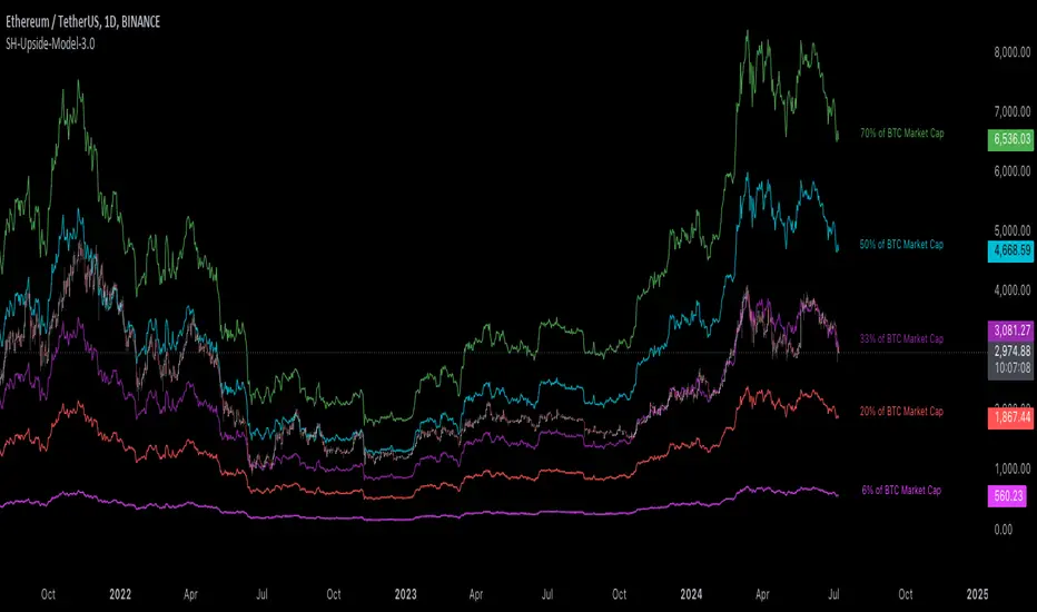
[Suitable Hope] Crypto Upside Model 3.0The "Crypto Upside Model 3.0" indicator dynamically calculates the potential price of any cryptocurrency based on various percentages of Ethereum or Bitcoin's market capitalization.
By fetching and analyzing marketcap data from TradingView sources, it allows traders to visualize potential price targets if their chosen cryptocurrency reaches specific market dominance levels. This tool is designed for daily timeframe analysis and can be used to set informed price expectations and strategic investment goals, providing valuable insights for long-term investment planning.
Why using the Crypto Upside Model 3.0?
Strategic Planning: Helps traders and investors set realistic price targets and investment goals by visualizing potential market cap scenarios.
Informed Decision-Making: Provides a data-driven approach to understanding how a cryptocurrency might perform relative to major assets like Bitcoin and Ethereum.
Customizable Analysis: Allows users to choose different comparison assets (ETH or BTC) and visualize various market cap dominance percentages, offering tailored insights.
Daily Timeframe Focus: Ideal for swing traders and long-term investors who operate on a daily analysis timeframe, providing relevant and actionable data.
Bull Markets: Identify potential price targets if your cryptocurrency's market cap increases significantly.
Bear Markets: Assess how much value could be retained relative to major cryptocurrencies.
Strategic Entry/Exit Points: Use the visualized targets to plan entry or exit points in your trading strategy.
Comparative Advantage
Dynamic Adaptation: Unlike fixed indicators, this tool adapts to any active chart, making it versatile for multiple cryptocurrencies.
Market Cap Insights: Provides a unique perspective by linking price targets to market cap dominance, a critical factor in the crypto market.
User Instructions
Setup: Add the " Upside Model 3.0" indicator to your TradingView chart.
Configuration: Use the input settings to select the comparison cryptocurrency (ETH or BTC) and enable the desired market cap percentage plots.
Analysis: The indicator will display potential price targets based on the selected market cap percentages, providing a visual guide for setting price expectations.
Limitations
Marketcap Data Availability: The indicator relies on marketcap data from TradingView, which may not be available for all cryptocurrencies. If the data is unavailable, the indicator will not function for that asset. This tool is more likely to work with older, established cryptocurrencies, as marketcap data for newer cryptocurrencies may not yet be available.
Daily Timeframe Restriction: The indicator is designed to work exclusively on the daily timeframe, limiting its applicability for intraday trading.
Assumptions of Market Dynamics: The calculations assume a direct correlation between market dominance and price, which may not account for other market dynamics and external factors influencing prices.
Data Accuracy: The accuracy of the indicator depends on the reliability of the data provided by TradingView, which may sometimes experience delays or inaccuracies.
Currently available cryptocurrencies: Bitcoin, Ethereum, Solana, Binance Coin, Cardano, Ripple, Polkadot, Avalanche, Chainlink, Litecoin, Dogecoin, Terra, Uniswap, VeChain, Stellar, Internet Computer, Hedera, Filecoin, Monero, Aave, TRON, NEAR Protocol, Compound, Maker,... For all compatible cryptocurrencies, please consult CRYPTOCAP's documentation.
Final notes
Although various sources ask a payment or user data for similar kind of private indicators, this one is entirely free and open source. "Uncanny" isn't it? I hope this indicator will provide you value. Feel free to leave a message if you have any questions or constructive feedback.
Examples of how I use this indicator
When using ETH's historical price as a reference compared to Bitcoin's marketcap, we can notice that price generally has been held between the +-30% and 50% lines of BTC's marketcap. If history is repeating again, we can expect major resistances around the 50% looking ahead into the future. This for me would be a great area to potentially reduce my ETH spot position.
When using SOL's historical price action, we can notice that the 15% line of ETH's marketcap has been a top in the previous cycle. Today SOL (July 2024), is back at this level. Could this be a top again or could price break this 15% level and head perhaps towards 30% which currently sits around $260? Time will tell.
These are 2 simple example of how I interpret the data. I'm keen to hear what other findings with other pairs you can find.
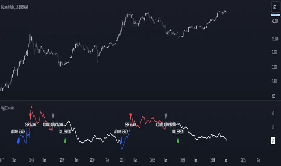
Crypto SeasonDefinition
This indicator is an informative indicator aiming to predict when the Altcoin season will start and when Bitcoin will enter the month season.
The average of the graph shows the dominance of altcoins other than BTC, ETH and USDT. If this value is over 30, the BTC says that the bull season is over. This value indicates that 20 to 30 BTC is in the bull season or accumulation. If this value is less than 20, it means that the subcoin season has begun.
Disclaimer
This indicator is for informational purposes only and should be used for educational purposes only. You may lose money if you rely on this to trade without additional information. Use at your own risk.
Version
v1.0
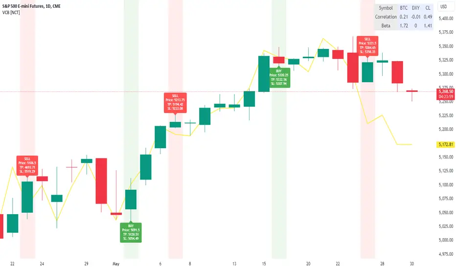
VolCorrBeta [NariCapitalTrading]Indicator Overview: VolCorrBeta
The VolCorrBeta indicator is designed to analyze and interpret intermarket relationships. This indicator combines volatility, correlation, and beta calculations to provide a comprehensive view of how certain assets (BTC, DXY, CL) influence the ES futures contract (I tailored this indicator to the ES contract, but it will work for any symbol).
Functionality
Input Symbols
BTCUSD : Bitcoin to USD
DXY : US Dollar Index
CL1! : Crude Oil Futures
ES1! : S&P 500 Futures
These symbols can be customized according to user preferences. The main focus of the indicator is to analyze how the price movements of these assets correlate with and lead the price movements of the ES futures contract.
Parameters for Calculation
Correlation Length : Number of periods for calculating the correlation.
Standard Deviation Length : Number of periods for calculating the standard deviation.
Lookback Period for Beta : Number of periods for calculating beta.
Volatility Filter Length : Length of the volatility filter.
Volatility Threshold : Threshold for adjusting the lookback period based on volatility.
Key Calculations
Returns Calculation : Computes the daily returns for each input symbol.
Correlation Calculation : Computes the correlation between each input symbol's returns and the ES futures contract returns over the specified correlation length.
Standard Deviation Calculation : Computes the standard deviation for each input symbol's returns and the ES futures contract returns.
Beta Calculation : Computes the beta for each input symbol relative to the ES futures contract.
Weighted Returns Calculation : Computes the weighted returns based on the calculated betas.
Lead-Lag Indicator : Calculates a lead-lag indicator by averaging the weighted returns.
Volatility Filter : Smooths the lead-lag indicator using a simple moving average.
Price Target Estimation : Estimates the ES price target based on the lead-lag indicator (the yellow line on the chart).
Dynamic Stop Loss (SL) and Take Profit (TP) Levels : Calculates dynamic SL and TP levels using volatility bands.
Signal Generation
The indicator generates buy and sell signals based on the filtered lead-lag indicator and confirms them using higher timeframe analysis. Signals are debounced to reduce frequency, ensuring that only significant signals are considered.
Visualization
Background Coloring : The background color changes based on the buy and sell signals for easy visualization (user can toggle this on/off).
Signal Labels : Labels with arrows are plotted on the chart, showing the signal type (buy/sell), the entry price, TP, and SL levels.
Estimated ES Price Target : The estimated price target for ES futures is plotted on the chart.
Correlation and Beta Dashboard : A table displayed in the top right corner shows the current correlation and beta values for relative to the ES futures contract.
Customization
Traders can customize the following parameters to tailor the indicator to their specific needs:
Input Symbols : Change the symbols for BTC, DXY, CL, and ES.
Correlation Length : Adjust the number of periods used for calculating correlation.
Standard Deviation Length : Adjust the number of periods used for calculating standard deviation.
Lookback Period for Beta : Change the lookback period for calculating beta.
Volatility Filter Length : Modify the length of the volatility filter.
Volatility Threshold : Set a threshold for adjusting the lookback period based on volatility.
Plotting Options : Customize the colors and line widths of the plotted elements.
TradingView.To Strategy Template (with Dyanmic Alerts)Hello traders,
If you're tired of manual trading and looking for a solid strategy template to pair with your indicators, look no further.
This Pine Script v5 strategy template is engineered for maximum customization and risk management.
Best part?
This Pine Script v5 template facilitates the dynamic construction of TradingView.TO alerts, sparing users the time and effort of mastering the TradingView.TO syntax and manually create alert commands.
This powerful tool gives much power to those who don't know how to code in Pinescript and want to automate their indicators' signals via TradingView.TO bot.
IMPORTANT NOTES
TradingView.TO is a trading bot software that forwards TradingView alerts to your brokers (examples: Binance, Oanda, Coinbase, Bybit, Metatrader 4/5, ...) for automating trading.
Many traders don't know how to create TradingView.TO dynamically-compatible alerts using the data from their TradingView scripts.
Traders using trading bots want their alerts to reflect the stop-loss/take-profit/trailing-stop/stop-loss to break options from your script and then create the orders accordingly.
This script showcases how to create TradingView.TO alerts dynamically.
TRADINGVIEW ALERTS
1) You'll have to create one alert per asset X timeframe = 1 chart.
Example: 1 alert for BTC/USDT on the 5 minutes chart, 1 alert for BTC/USDT on the 15-minute chart (assuming you want your bot to trade the BTC/USDT on the 5 and 15-minute timeframes)
2) Select the Order fills and alert() function calls condition
3) For each alert, the alert message is pre-configured with the text below
{{strategy.order.alert_message}}
Please leave it as it is.
It's a TradingView native variable that will fetch the alert text messages built by the script.
4) TradingView.TO uses webhook technology - setting a webhook URL from the alerts notifications tab is required.
KEY FEATURES
I) Modular Indicator Connection
* plug your existing indicator into the template.
* Only two lines of code are needed for full compatibility.
Step 1: Create your connector
Adapt your indicator with only 2 lines of code and then connect it to this strategy template.
To do so:
1) Find in your indicator where the conditions print the long/buy and short/sell signals.
2) Create an additional plot as below
I'm giving an example with a Two moving averages cross.
Please replicate the same methodology for your indicator, whether a MACD , ZigZag, Pivots , higher-highs, lower-lows or whatever indicator with clear buy and sell conditions.
//@version=5
indicator("Supertrend", overlay = true, timeframe = "", timeframe_gaps = true)
atrPeriod = input.int(10, "ATR Length", minval = 1)
factor = input.float(3.0, "Factor", minval = 0.01, step = 0.01)
= ta.supertrend(factor, atrPeriod)
supertrend := barstate.isfirst ? na : supertrend
bodyMiddle = plot(barstate.isfirst ? na : (open + close) / 2, display = display.none)
upTrend = plot(direction < 0 ? supertrend : na, "Up Trend", color = color.green, style = plot.style_linebr)
downTrend = plot(direction < 0 ? na : supertrend, "Down Trend", color = color.red, style = plot.style_linebr)
fill(bodyMiddle, upTrend, color.new(color.green, 90), fillgaps = false)
fill(bodyMiddle, downTrend, color.new(color.red, 90), fillgaps = false)
buy = ta.crossunder(direction, 0)
sell = ta.crossunder(direction, 0)
//////// CONNECTOR SECTION ////////
Signal = buy ? 1 : sell ? -1 : 0
plot(Signal, title = "Signal", display = display.data_window)
//////// CONNECTOR SECTION ////////
Important Notes
🔥 The Strategy Template expects the value to be exactly 1 for the bullish signal and -1 for the bearish signal
Now, you can connect your indicator to the Strategy Template using the method below or that one.
Step 2: Connect the connector
1) Add your updated indicator to a TradingView chart
2) Add the Strategy Template as well to the SAME chart
3) Open the Strategy Template settings, and in the Data Source field, select your 🔌Connector🔌 (which comes from your indicator)
Note it doesn’t have to be named 🔌Connector🔌 - you can name it as you want - however, I recommend an explicit name you can easily remember.
From then, you should start seeing the signals and plenty of other stuff on your chart.
🔥 Note that whenever you update your indicator values, the strategy statistics and visuals on your chart will update in real-time
II) BOT Risk Management:
- Max Drawdown:
Mode: Select whether the max drawdown is calculated in percentage (%) or USD.
Value: If the max drawdown reaches this specified value, set a value to halt the bot.
- Max Consecutive Days:
Use Max Consecutive Days BOT Halt: Enable/Disable halting the bot if the max consecutive losing days value is reached.
- Max Consecutive Days: Set the maximum number of consecutive losing days allowed before halting the bot.
- Max Losing Streak:
Use Max Losing Streak: Enable/Disable a feature to prevent the bot from taking too many losses in a row.
- Max Losing Streak Length: Set the maximum length of a losing streak allowed.
Margin Call:
- Use Margin Call: Enable/Disable a feature to exit when a specified percentage away from a margin call to prevent it.
Margin Call (%): Set the percentage value to trigger this feature.
- Close BOT Total Loss:
Use Close BOT Total Loss: Enable/Disable a feature to close all trades and halt the bot if the total loss is reached.
- Total Loss ($): Set the total loss value in USD to trigger this feature.
Intraday BOT Risk Management:
- Intraday Losses:
Use Intraday Losses BOT Halt: Enable/Disable halting the bot on reaching specified intraday losses.
Mode: Select whether the intraday loss is calculated in percentage (%) or USD.
- Max Intraday Losses (%): Set the value for maximum intraday losses.
Limit Intraday Trades:
- Use Limit Intraday Trades: Enable/Disable a feature to limit the number of intraday trades.
- Max Intraday Trades: Set the maximum number of intraday trades allowed.
Restart Intraday EA:
III) Order Types and Position Sizing
- Choose between market or limit orders.
- Set your position size directly in the template.
Please use the position size from the “Inputs” and not the “Properties” tab.
I know it's redundant. - the template needs this value from the "Inputs" tab to build the alerts, and the Backtester needs it from the "Properties" tab.
IV) Advanced Take-Profit and Stop-Loss Options
- Choose to set your SL/TP in either USD or percentages.
- Option for multiple take-profit levels and trailing stop losses.
- Move your stop loss to break even +/- offset in USD for “risk-free” trades.
V) Miscellaneous:
Retry order openings if they fail.
Order Types:
Select and specify order type and price settings.
Position Size:
Define the type and size of positions.
Leverage:
Leverage settings, including margin type and hedge mode.
Session:
Limit trades to specific sessions.
Dates:
Limit trades to a specific date range.
Trades Direction:
Direction: Specify the market direction for opening positions.
VI) Logger
The TradingView.TO commands are logged in the TradingView logger.
You'll find more information about it in this TradingView blog post .
WHY YOU MIGHT NEED THIS TEMPLATE
1) Transform your indicator into a TradingView.TO trading bot more easily than before
Connect your indicator to the template
Create your alerts
Set your EA settings
2) Save Time
Auto-generated alert messages for TradingView.TO.
I tested them all and checked with the support team what could/couldn’t be done.
3) Be in Control
Manage your trading risks with advanced features.
4) Customizable
Fits various trading styles and asset classes.
REQUIREMENTS
* Make sure you have your TradingView.TO account
* If there is any issue with the template, ask me in the comments section - I’ll answer quickly.
BACKTEST RESULTS FROM THIS POST
1) I connected this strategy template to a dummy Supertrend script.
I could have selected any other indicator or concept for this script post.
I wanted to share an example of how you can quickly upgrade your strategy, making it compatible with TradingView.TO.
2) The backtest results aren't relevant for this educational script publication.
I used realistic backtesting data but didn't look too much into optimizing the results, as this isn't the point of why I'm publishing this script.
This strategy is a template to be connected to any indicator - the sky is the limit. :)
3) This template is made to take 1 trade per direction at any given time.
Pyramiding is set to 1 on TradingView.
The strategy default settings are:
* Initial Capital: 100000 USD
* Position Size: 1%
* Commission Percent: 0.075%
* Slippage: 1 tick
* No margin/leverage used

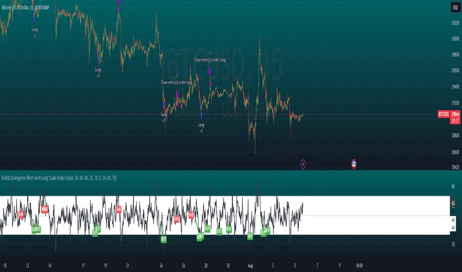
Bullish Divergence Short-term Long Trade FinderThis script is a Bullish divergence trade finder built to find small periods where Bitcoin will likely rise from. It looks for bullish divergence followed by a higher low as long as the hour RSI value is below the 40 mark, if then it will enter an long. It marks out Buy signals on the RSI if the value dips below 'RSI Bull Condition Minimum' (Default 40) on the current time frame in view. It also marks out Sell signals found when the RSI is above the 'RSI Bearish Condition Minimum' (Default 50). The sell signals are bearish divergence that has occurred recently on the RSI. When a long is in play it will sell if it finds bearish divergence or the time frame in view reaches RSI value higher than the 'RSI Sell Value'(Default 75). You can set your stop loss value with the 'Stop loss Percentage' (default 5).
Available inputs:
RSI Period: relative strength measurement length(Typically 14)
RSI Oversold Level: the bottom bar of the RSI (Typically 30)
RSI Overbought Level: the top bar of the RSI (Typically 70)
RSI Bearish Condition Minimum: The minimum value the script will use to look for a pivot high that starts the Bearish condition to Sell (Default 50)
RSI Bearish Condition Sell Min: the minimum value the script will accept a bearish condition (Default 60)
RSI Bull Condition Minimum: the minimum value it will consider a pivot low value in the RSI to find a divergence buy (Default 40)
Look Back this many candles: the amount of candles thee script will look back to find a low value in the RSI (Default 25)
RSI Sell Value: The RSI value of the exit condition for a long when value is reached (Default 75)
Stop loss Percentage: Percentage value for amount to lose (Default 5)
The formula to enter a long is stated below:
If price finds a lower low and there is a higher low found following a lower low and price has just made another dip and price closes lower than the last divergence and Relative strength index hour value is less than 40 enter a long.
The formula to exit a long is stated below:
If the value drops below the stop loss percentage OR (the RSI value is greater than the value of the parameter 'RSI Sell Value' or bearish divergence is found greater than the parameter 'RSI Bearish Condition Minimum' )
This script was built from much strategy testing on BTC but works with alts (occasionally) also. It is most successful to my knowledge using the 15 min and 7 min time frames with default values. Hope it helps! Follow for further possible updates to this script or other entry or exit strategies.
snapshot:
I only have a Pro trading view account so I cannot share a larger data set about this script because the buy signals happen pretty rarely. The most amount that I could find within a view for me was 40 trades within a viewable time. The suggested/default parameters that I have do not occur very often so it limits the data set. Adjustments can be made to the parameters so that trades can be entered more often. The scripts success is dependent on the values of the parameters set by the user. This script was written to be used for BTC/USD or BTC/USDT trading. I am unable to share a larger dataset without putting out results that are intended to fail or having a premium account so reaching the 100 trade minimum is not possible with my account.
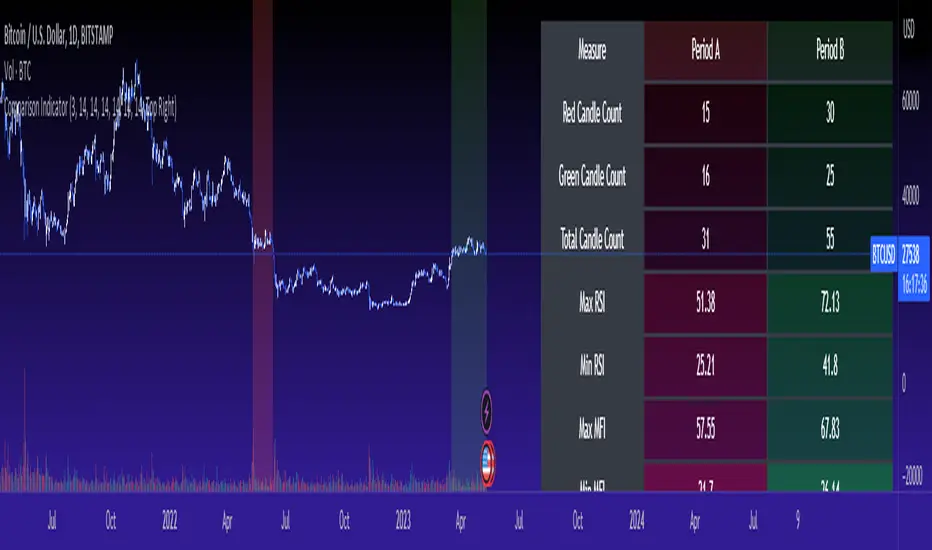
Cross Period Comparison IndicatorReally excited to be sharing this indicator!
This is the cross-period comparison indicator, AKA the comparison indicator.
What does it do?
The cross-period comparison indicator permits for the qualitative assessment of two points in time on a particular equity.
What is its use?
At first, I was looking for a way to determine the degree of similarity between two points, such as using Cosine similarity values, Euclidean distances, etc. However, these tend to trigger a lot of similarities but without really any context. Context matters in trading and thus what I wanted really was a qualitative assessment tool to see what exactly was happening at two points in time (i.e. How many buyers were there? What was short interest like? What was volume like? What was the volatility like? RSI? Etc.)
This indicator permits that qualitative assessment, displaying things like total buying volume during each period, total selling volume, short interest via Put to Call ratio activity, technical information such as Stochastics and RSI, etc.
How to use it?
The indicator is fairly self explanatory, but some things require a little more in-depth discussion.
The indicator will display the Max and Min technical values of a period, as well as a breakdown in the volume information and put to call information. The user can then make the qualitative determination of degrees of similarity. However, I have included some key things to help ascertain similarity in a more quantitative way. These include:
1. Adding average period Z-Score
2. Adding CDF probability distributions for each respective period
3. Adding Pearson correlations for each respective period over time
4. Providing the linear regression equation for each period
So let us discuss these 4 quantitative measures a bit more in-depth.
Adding Period Z-Score
For those who do not know, Z-Score is a measure of the distance from a mean. It generally spans 0 (at the mean) to 3 (3 standard deviations away from the mean). Z-Score in the stock market is very powerful because it is actually our indicator of volatility. Z-Score forms the basis of IV for option traders and it generally is the go to, to see where the market is in relation to its overall mean.
Adding Z-Score lets the user make 2 big determinations. First and foremost, it’s a measure of overall volatility during the period. If you are getting a Z-Score that is crazy high (1.5 or greater), you know there was a lot of volatility in that period marked by frequent deviations from its mean (since on average it was trading 1.5 standard deviations away from its mean).
The other thing it tells you is the overall sentiment of that time. If the average Z Score was 1.5 for example, we know that buying interest was high and the sentiment was somewhat optimistic, as the stock was trading, on average, + 1.5 SDs away from its mean.
If, on the other hand, the average was, say, - 1.2, then we know the sentiment was overall pessimistic. There was frequent selling and the stock was frequently being pushed below its mean with heavy selling pressure.
We can also check these assumptions of buying / selling buy verifying the volume information. The indicator will list the Buy to Sell Ratio (number of Buyers to Sellers), as well as the total selling volume and total buying volume. Thus, the user can see, objectively, whether sellers or buyers led a particular period.
Adding CDF Probability
CDF probabilities simply mean the extent a stock traded above or below its normal distribution levels.
To help you understand this, the indicator lists the average close price for a period. Directly below that, it lists the CDF probabilities. What this is telling you, is how often and how likely, during that period, the stock was trading below its average. For example, in the main chart, the average close price for BTC in Period A is 29869. The CDF probability is 0.51. This means, during Period A, 51% of the time, BTC was trading BELOW 29869. Thus, the other 49% of the time it was trading ABOVE 29869.
CDF probabilities also help us to assess volatility, similar to Z-Score. Generally speaking, the CDF should consistently be reading about 0.50 to 0.51. This is the point of an average value, half the values should be above the average and half the values should be below. But in times of heightened volatility, you may actually see the CDF creep up to 0.54 or higher, or 0.48 or lower. This means that there was extremely extensive volatility and is very indicative of true “whipsaw” type price action history where a stock refuses to average itself out in one general area and frequently jumps up and down.
Adding Pearson Correlation
Most know what this is, but just in case, the Pearson correlation is a measure of statistical significance. It ranges from 0 (not significant) to 1 (very significant). It can be positive or negative. A positive signifies a positive relationship (i.e. as one value increases so too does the other value being compared). If it is a negative value, it means an inverse relationship (i.e. one value increases proportionately to the other’s decline).
In this indicator, the Pearson correlation is measured against time. A strong positive relationship (a value of 0.5 or greater) indicates that the stock is trading positive to time. As time goes by, the stock goes up. This is a normal relationship and signifies a healthy uptrend.
Inversely, if the Pearson correlation is negative, it means that as time increases, the stock is going down proportionately. This signifies a strong downtrend.
This is another way for the user to interpret sentiment during a specific period.
IF the Pearson correlation is less than 0.5 or -0.5, this signifies an area of indecision. No real trend formed and there was no real strong relationship to time.
Adding Linear Regression Equation
A linear regression equation is simply the slope and the intercept. It is expressed with the formula y= mx + b.
The indicator does a regression analysis on each period and presents this formula accordingly. The user can see the slope and intercept.
Generally speaking, when two periods share the same slope (m value) but different intercept (b value), it can be said that the relationship to time is identical but the starting point is different.
If the slope and intercept are different, as you see in the BTC chart above, it represents a completely different relationship to time and trajectory.
Indicator Specific Information:
The indicator retains the customizability you would expect. You can customize all of your lengths for technical, change and Z-Score. You can toggle on or off Period data, if you want to focus on a single period. You can also toggle on a difference table that directly compares the % difference between Period A to Period B (see image below):
You will also see on the input menu a input for “Threshold” assessments. This simply modifies the threshold parameters for the technical readings. It is defaulted to 3, which means when two technical (for example Max Stochastics) are within +/- 3 of each other, the indicator will light these up as green to indicate similarities. They just clue the user visually to areas where there are similarities amongst the qualitative technical data.
Timeframes
This is best used on the daily timeframe. You can use it on the smaller timeframe but the processing time may take a bit longer. I personally like it for the Daily, Weekly and 4 hour charts.
And this is the indicator in a nutshell!
I will provide a tutorial video in the coming day on how to use it, so check back later!
As always, leave your comments/questions and suggestions below. I have been slowly modifying stuff based on user suggestions so please keep them coming but be patient as it does take some time and I am by no means a coder or expert on this stuff.
Safe trades to all!
Typical Price Difference - TPD © with reversal zones and signalsv1.0 NOTE: The maths have been tested only for BTC and weekly time frame.
This is a concept that I came through after long long hours of VWAP trading and scalping.
The idea is pretty simple:
1) Typical Price is calculated by (h+l+c) / 3. If we take this price and adjust it to volume we get the VWAP value. The difference between this value and the close value, i call it " Typical Price Difference - TPD ".
2) We get the Historical Volatility as calculated by TradingView script and we add it up to TPD and divide it by two (average). This is what I call " The Source - TS ".
3) We apply the CCI formula to TS .
4) We calculate the Rate of Change (roc) of the CCI formula.
5) We apply the VIX FIX of Larry Williams (script used is from ChrisMoody - CM_Williams_Vix_Fix Finds Market Bottoms) *brilliant script!!!
How to use it:
a) When the (3) is over the TPD we have a bullish bias (green area). When it's under we have a bearish bias (red area).
b) If the (1) value goes over or under a certain value (CAUTION!!! it varies in different assets or timeframes) we get a Reversal Zone (RZ). Red/Green background.
c) If we are in a RZ and the VIX FIX gives a strong value (look for green bars in histogram) and roc (4) goes in the opposite direction, we get a reversal signal that works for the next week(s).
I applied this to BTC on a weekly time frame and after some corrections, it gives pretty good reversal zones and signals. Especially bottoms. Also look for divergences in the zones/signals.
As I said I have tested and confirmed it only on BTC/weekly. I need more time with the maths and pine to automatically adjust it to other time frames. You can play with it in different assets or time frames to find best settings by hand.
Feel free to share your thoughts or ideas on this.
P.S. I realy realy realy try to remember when or how or why I came up with the idea to combine typical price with historical volatility and CCI. I can't! It doesn't make any sense LOL

Kimchi Premium watchThis indicator provides easy-to-see Kimchi premium information.
It provides three pieces of information.
1. Current premium
2. The highest value of the premium over the last 240 candlesticks in the current timeframe.
3. The highest value of the premium over the last 240 candlesticks in the current timeframe.
I think this script is a very simple indicator.
It is usually recommended to get value in a large time frame.
The basic operation formula is as follows.
premium(percent) = ( BTC KRW - ( BTC USDT x USD KRW ) / ( BTC USDT x USDT USD x USD KRW )) x 100
Thank you.