Aethix Cipher DivergencesAethix Cipher Divergences v6
Core Hook: Custom indicator inspired by VuManChu B, Grok-enhanced for crypto intel—blends WaveTrend (WT) oscillator with multi-divergences for buy/sell circles (green/teal buys #00FFFF, red sells) and dots (divs, gold overbought alerts).
Key Features:
WaveTrend Waves: Dual waves (teal WT1, darker teal WT2) with VWAP (purple for neon vibe), overbought/oversold lines, crosses for signals.
Divergences: Regular/hidden for WT, RSI, Stoch—red bearish, green bullish dots; extra range for deeper insights.
RSI + MFI Area: Colored area (green positive, red negative) for sentiment/volume flow.
Stochastic RSI: K/D lines with fill for overbought/oversold trends.
Schaff Trend Cycle: Purple line for cycle smoothing.
Sommi Patterns: Flags (pink bearish, blue bullish) and diamonds for HTF patterns, purple higher VWAP.
MACD Colors on WT: Dynamic WT shading based on MACD for enhanced reads.
Cerca negli script per "deep股票代码"

VWAP Bands Pro - Session Based by kobiko3030
📊 Advanced Professional Trading Indicator
VWAP Bands Pro is an advanced indicator that combines the power of VWAP with 4 dynamic bands for precise identification of support and resistance zones. This indicator is designed for professional traders who want deep and accurate market movement analysis.
✨ Key Features
🎯 Smart VWAP Bands
4 adjustable bands based on standard deviation
Optional band 4 hiding for beginner traders
Precise calculation based on volume-weighted price
🌏 Global Session Support
New York Session (9:30 EST)
Asia Session (18:00 EST)
Automatic reset at the beginning of each session
📱 Flexible User Interface
Dynamic labels (V, VR1-4, VS1-4)
Custom color selection
Adjustable line thickness for each band
Multiple display modes
🔔 Advanced Alert System
VWAP breakout alerts
Alerts for all bands (3 & 4)
Clear and precise messages
🛠️ Customization Options
Band Settings
Standard deviation multipliers: 1.0, 2.0, 3.0, 4.0 (default)
Each band independently adjustable
Range: 0.1 to 5.0
Display Settings
Continuous trading start - display from session beginning
Limited candle count - show last X candles
Current day only - no historical data
Visual Design
VWAP, support, and resistance colors
Individual line thickness
Hideable labels
📈 Trading Strategies
Support and Resistance Zones
VS1-VS4: Support bands (green)
VR1-VR4: Resistance bands (red)
V: Central VWAP line
Entry Points
Breakouts above/below VWAP
Bounces from outer bands
Band retests
Risk Management
Use bands as Stop Loss levels
Identify oversold/overbought zones
Adapt to different market conditions
🎖️ Indicator Advantages
✅ Precise calculation based on volume weighting
✅ Complete flexibility in customization
✅ Global session support
✅ User-friendly interface
✅ Built-in alert system
✅ Suitable for all trading styles
📋 Usage Instructions
Add the indicator to your chart
Select trading session (New York/Asia)
Adjust bands according to your trading style
Set up alerts for important breakouts
Start trading with precise key zone identification
💡 Trading Tips
Use outer bands to identify extremes
Combine with additional indicators for confirmation
Adjust bands to asset volatility
Follow alerts to spot opportunities
Consider session-specific behavior patterns
🔧 Technical Specifications
Pine Script Version: 5
Overlay: Yes
Timeframe: All timeframes supported
Markets: Suitable for all markets (Forex, Stocks, Crypto, Futures)
Session Support: New York & Asia with EST timezone
Volume Calculation: HLC3 * Volume weighted
📊 What Makes This Different
Unlike standard VWAP indicators, this pro version offers:
Session-based reset for intraday precision
4 customizable bands instead of basic 2
Professional labeling system for quick identification
Advanced alert conditions for all key levels
Flexible display options for different trading approaches
⚡ Performance Features
Efficient calculation - minimal lag
Clean visual design - no chart clutter
Responsive labels - update in real-time
Session breaks - clear visual separation
Volume validation - ensures accurate VWAP calculation

Information-Geometric Market DynamicsInformation-Geometric Market Dynamics
The Information Field: A Geometric Approach to Market Dynamics
By: DskyzInvestments
Foreword: Beyond the Shadows on the Wall
If you have traded for any length of time, you know " the feeling ." It is the frustration of a perfect setup that fails, the whipsaw that stops you out just before the real move, the nagging sense that the chart is telling you only half the story. For decades, technical analysis has relied on interpreting the shadows—the patterns left behind by price. We draw lines on these shadows, apply indicators to them, and hope they reveal the future.
But what if we could stop looking at the shadows and, instead, analyze the object casting them?
This script introduces a new paradigm for market analysis: Information-Geometric Market Dynamics (IGMD) . The core premise of IGMD is that the price chart is merely a one-dimensional projection of a much richer, higher-dimensional reality—an " information field " generated by the collective actions and beliefs of all market participants.
This is not just another collection of indicators. It is a unified framework for measuring the geometry of the market's information field—its memory, its complexity, its uncertainty, its causal flows—and making high-probability decisions based on that deeper reality. By fusing advanced mathematical and informational concepts, IGMD provides a multi-faceted lens through which to view market behavior, moving beyond simple price action into the very structure of market information itself.
Prepare to move beyond the flatland of the price chart. Welcome to the information field.
The IGMD Framework: A Multi-Kernel Approach
What is a Kernel? The Heart of Transformation
In mathematics and data science, a kernel is a powerful and elegant concept. At its core, a kernel is a function that takes complex, often inscrutable data and transforms it into a more useful format. Think of it as a specialized lens or a mathematical "probe." You cannot directly measure abstract concepts like "market memory" or "trend quality" by looking at a price number. First, you must process the raw price data through a specific mathematical machine—a kernel—that is designed to output a measurement of that specific property. Kernels operate by performing a sort of "similarity test," projecting data into a higher-dimensional space where hidden patterns and relationships become visible and measurable.
Why do creators use them? We use kernels to extract features —meaningful pieces of information—that are not explicitly present in the raw data. They are the essential tools for moving beyond surface-level analysis into the very DNA of market behavior. A simple moving average can tell you the average price; a suite of well-chosen kernels can tell you about the character of the price action itself.
The Alchemist's Challenge: The Art of Fusion
Using a single kernel is a challenge. Using five distinct, computationally demanding mathematical engines in unison is an immense undertaking. The true difficulty—and artistry—lies not just in using one kernel, but in fusing the outputs of many . Each kernel provides a different perspective, and they can often give conflicting signals. One kernel might detect a strong trend, while another signals rising chaos and uncertainty. The IGMD script's greatest strength is its ability to act as this alchemist, synthesizing these disparate viewpoints through a weighted fusion process to produce a single, coherent picture of the market's state. It required countless hours of testing and calibration to balance the influence of these five distinct analytical engines so they work in harmony rather than cacophony.
The Five Kernels of Market Dynamics
The IGMD script is built upon a foundation of five distinct kernels, each chosen to probe a unique and critical dimension of the market's information field.
1. The Wavelet Kernel (The "Microscope")
What it is: The Wavelet Kernel is a signal processing function designed to decompose a signal into different frequency scales. Unlike a Fourier Transform that analyzes the entire signal at once, the wavelet slides across the data, providing information about both what frequencies are present and when they occurred.
The Kernels I Use:
Haar Kernel: The simplest wavelet, a square-wave shape defined by the coefficients . It excels at detecting sharp, sudden changes.
Daubechies 2 (db2) Kernel: A more complex and smoother wavelet shape that provides a better balance for analyzing the nuanced ebb and flow of typical market trends.
How it Works in the Script: This kernel is applied iteratively. It first separates the finest "noise" (detail d1) from the first level of trend (approximation a1). It then takes the trend a1 and repeats the process, extracting the next level of cycle (d2) and trend (a2), and so on. This hierarchical decomposition allows us to separate short-term noise from the long-term market "thesis."
2. The Hurst Exponent Kernel (The "Memory Gauge")
What it is: The Hurst Exponent is derived from a statistical analysis kernel that measures the "long-term memory" or persistence of a time series. It is the definitive measure of whether a series is trending (H > 0.5), mean-reverting (H < 0.5), or random (H = 0.5).
How it Works in the Script: The script employs a method based on Rescaled Range (R/S) analysis. It calculates the average range of price movements over increasingly larger time lags (m1, m2, m4, m8...). The slope of the line plotting log(range) vs. log(lag) is the Hurst Exponent. Applying this complex statistical analysis not to the raw price, but to the clean, wavelet-decomposed trend lines, is a key innovation of IGMD.
3. The Fractal Dimension Kernel (The "Complexity Compass")
What it is: This kernel measures the geometric complexity or "jaggedness" of a price path, based on the principles of fractal geometry. A straight line has a dimension of 1; a chaotic, space-filling line approaches a dimension of 2.
How it Works in the Script: We use a version based on Ehlers' Fractal Dimension Index (FDI). It calculates the rate of price change over a full lookback period (N3) and compares it to the sum of the rates of change over the two halves of that period (N1 + N2). The formula d = (log(N1 + N2) - log(N3)) / log(2) quantifies how much "longer" and more convoluted the price path was than a simple straight line. This kernel is our primary filter for tradeable (low complexity) vs. untradeable (high complexity) conditions.
4. The Shannon Entropy Kernel (The "Uncertainty Meter")
What it is: This kernel comes from Information Theory and provides the purest mathematical measure of information, surprise, or uncertainty within a system. It is not a measure of volatility; a market moving predictably up by 10 points every bar has high volatility but zero entropy .
How it Works in the Script: The script normalizes price returns by the ATR, categorizes them into a discrete number of "bins" over a lookback window, and forms a probability distribution. The Shannon Entropy H = -Σ(p_i * log(p_i)) is calculated from this distribution. A low H means returns are predictable. A high H means returns are chaotic. This kernel is our ultimate gauge of market conviction.
5. The Transfer Entropy Kernel (The "Causality Probe")
What it is: This is by far the most advanced and computationally intensive kernel in the script. Transfer Entropy is a non-parametric measure of directed information flow between two time series. It moves beyond correlation to ask: "Does knowing the past of Volume genuinely reduce our uncertainty about the future of Price?"
How it Works in the Script: To make this work, the script discretizes both price returns and the chosen "driver" (e.g., OBV) into three states: "up," "down," or "neutral." It then builds complex conditional probability tables to measure the flow of information in both directions. The Net Transfer Entropy (TE Driver→Price minus TE Price→Driver) gives us a direct measure of causality . A positive score means the driver is leading price, confirming the validity of the move. This is a profound leap beyond traditional indicator analysis.
Chapter 3: Fusion & Interpretation - The Field Score & Dashboard
Each kernel is a specialist providing a piece of the puzzle. The Field Score is where they are fused into a single, comprehensive reading. It's a weighted sum of the normalized scores from all five kernels, producing a single number from -1 (maximum bearish information field) to +1 (maximum bullish information field). This is the ultimate "at-a-glance" metric for the market's net state, and it is interpreted through the dashboard.
The Dashboard: Your Mission Control
Field Score & Regime: The master metric and its plain-English interpretation ("Uptrend Field", "Downtrend Field", "Transitional").
Kernel Readouts (Wave Align, H(w), FDI, etc.): The live scores of each individual kernel. This allows you to see why the Field Score is what it is. A high Field Score with all components in agreement (all green or red) is a state of High Coherence and represents a high-quality setup.
Market Context: Standard metrics like RSI and Volume for additional confluence.
Signals: The raw and adjusted confluence counts and the final, calculated probability scores for potential long and short entries.
Pattern: Shows the dominant candlestick pattern detected within the currently forming APEX range box and its calculated confidence percentage.
Chapter 4: Mastering the Controls - The Inputs Menu
Every parameter is a lever to fine-tune the IGMD engine.
📊 Wavelet Transform: Kernel ( Haar for sharp moves, db2 for smooth trends) and Scales (depth of analysis) let you tune the script's core microscope to your asset's personality.
📈 Hurst Exponent: The Window determines if you're assessing short-term or long-term market memory.
🔍 Fractal Dimension & ⚡ Entropy Volatility: Adjust the lookback windows to make these kernels more or less sensitive to recent price action. Always keep "Normalize by ATR" enabled for Entropy for consistent results.
🔄 Transfer Entropy: Driver lets you choose what causal force to measure (e.g., OBV, Volume, or even an external symbol like VIX). The throttle setting is a crucial performance tool, allowing you to balance precision with script speed.
⚡ Field Fusion • Weights: This is where you can customize the model's "brain." Increase the weights for the kernels that best align with your trading philosophy (e.g., w_hurst for trend followers, w_fdi for chop avoiders).
📊 Signal Engine: Mode offers presets from Conservative to Aggressive . Min Confluence sets your evidence threshold. Dynamic Confluence is a powerful feature that automatically adapts this threshold to the market regime.
🎨 Visuals & 📏 Support/Resistance: These inputs give you full control over the chart's appearance, allowing you to toggle every visual element for a setup that is as clean or as data-rich as you desire.
Chapter 5: Reading the Battlefield - On-Chart Visuals
Pattern Boxes (The Large Rectangles): These are not simple range boxes. They appear when the Field Score crosses a significance threshold, signaling a potential ignition point.
Color: The color reflects the dominant candlestick pattern that has occurred within that box's duration (e.g., green for Bull Engulf).
Label: Displays the dominant pattern, its duration in bars, and a calculated Confidence % based on field strength and pattern clarity.
Bar Pattern Boxes (The Small Boxes): If enabled, these highlight individual, significant candlestick patterns ( BE for Bull Engulf, H for Hammer) on a bar-by-bar basis.
Signal Markers (▲ and ▼): These appear only when the Signal Engine's criteria are all met. The number is the calculated Probability Score .
RR Rails (Dashed Lines): When a signal appears, these lines automatically plot the Entry, Stop Loss (based on ATR), and two Take Profit targets (based on Risk/Reward ratios). They dynamically break and disappear as price touches each level.
Support & Resistance Lines: Plots of the highest high ( Resistance ) and lowest low ( Support ) over a lookback, providing key structural levels.
Chapter 6: Development Philosophy & A Final Word
One single question: " What is the market really doing? " It represents a triumph of complexity, blending concepts from signal processing, chaos theory, and information theory into a cohesive framework. It is offered for educational and analytical purposes and does not constitute financial advice. Its goal is to elevate your analysis from interpreting flat shadows to measuring the rich, geometric reality of the market's information field.
As the great mathematician Benoit Mandelbrot , father of fractal geometry, noted:
"Clouds are not spheres, mountains are not cones, coastlines are not circles, and bark is not smooth, nor does lightning travel in a straight line."
Neither does the market. IGMD is a tool designed to navigate that beautiful, complex, and fractal reality.
— Dskyz, Trade with insight. Trade with anticipation.

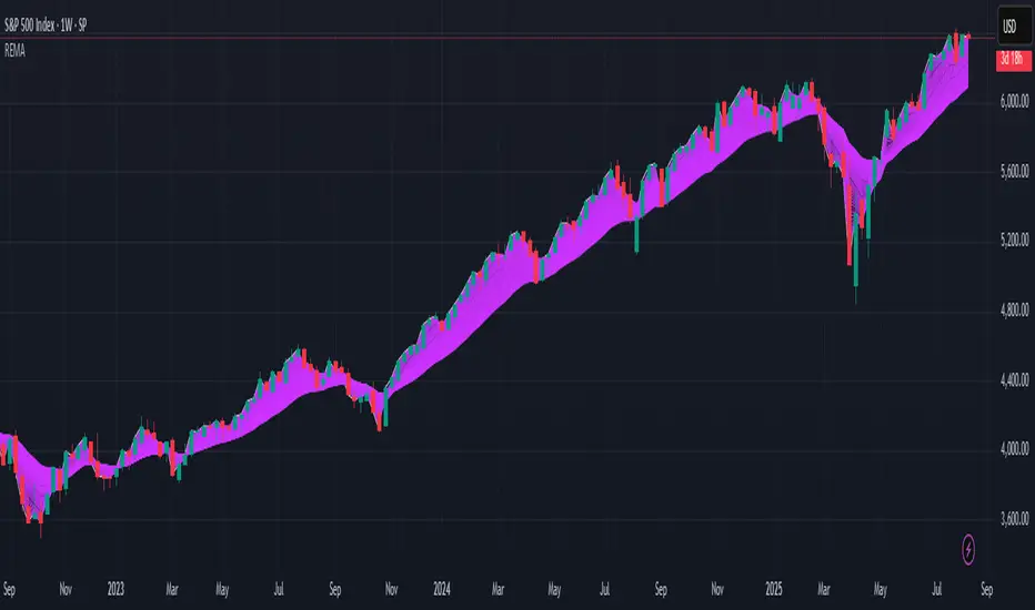
Fabian Z-ScoreFabian Z-Score — % Distance & Z-Scores for SPX / DJI / XLU
What it does
This indicator measures how far three market proxies are from a moving average and standardizes those distances into z-scores so you can spot stretch/mean-reversion and relative out/under-performance.
Universe: S&P 500 (SPX), Dow Jones (DJI) and Utilities (XLU). You can change any of these in Inputs.
Anchor MA: user-selectable MA type (SMA/EMA/RMA/WMA/VWMA/HMA/LSMA/ALMA) and length (default 39; a popular weekly anchor).
Outputs
% from MA: 100 × (𝐶𝑙𝑜𝑠𝑒 − 𝑀𝐴) / 𝑀𝐴
Time-series Z: z-score of the last N % distances (default 39) → “how stretched vs its own history?”
Cross-sectional Z: z-score of each % distance within the trio on this bar → “who’s strongest vs the others right now?”
A compact mini table (top-right) shows the latest values for each symbol: % from MA, Z(ts) and Z(xsec).
Panels & Visualization
Toggle what you want to see in View:
Plot % distance — raw % above/below the MA (0% line shown).
Plot time-series Z — standardized stretch with ±Threshold guides (default ±2σ).
Plot cross-sectional Z — relative z across SPX, DJI, XLU (0 = at the trio’s mean).
Smoothing — optional light MA on the plotted series (set to 1 for none).
A price-panel Moving Average is drawn with your chosen type/length for visual context.
Colors: SPX = teal, DJI = orange, XLU = purple.
Alerts
Two built-in alert conditions (time-series Z only):
“Z(ts) crosses up +Thr” — any of the three crosses above +Threshold.
“Z(ts) crosses down -Thr” — any crosses below −Threshold.
When enabled, the chart background tints faint green (up cross) or red (down cross) on those bars.
How to use (ideas, not advice)
On weekly charts, a 39-length MA/Z lookback often captures major risk-on/off swings. (Fabian Timing)
Deep negative Z(ts) (e.g., ≤ −2σ or −3σ) frequently accompanies panic and mean-reversion setups.
High positive Z(ts) suggests over-extension; watch for momentum fades.
Cross-sectional Z helps rank leadership today:
Z(xsec) > 0 → stronger than the trio’s mean this bar; Z(xsec) < 0 → weaker.
Utilities (XLU) turning positive x-sec while the others are negative can hint at defensive rotation.
If all 3 are above 0, go long, if below 0 go cash.
Combine: look for extreme Z(ts) aligning with lead/lag Z(xsec) to time entries/exits or hedges.
Inputs (quick reference)
Symbols: SPX / DJI / XLU (editable).
MA type & length: SMA, EMA, RMA, WMA, VWMA, HMA, LSMA, ALMA; default EMA(39).
Z-score lookback (ts): default 39.
Smoothing on plots: default 1 (off).
Z threshold (±): default 2.0 (guide lines & alerts).

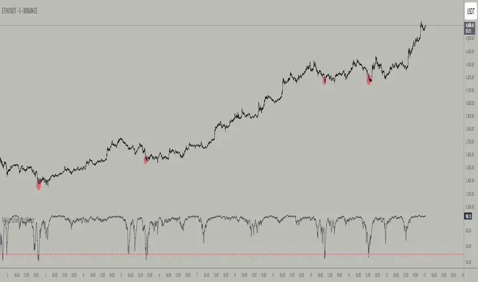
Major Lows OscillatorDescription
The Major Lows Oscillator is a custom technical indicator designed to identify significant low-price areas by normalizing the current closing price relative to recent lowest lows and highest highs. The oscillator calculates a normalized price percentage over a configurable lookback period, applies exponential moving averages for smoothing, and inverts the result to highlight potential market bottoms.
Calculation Details
Lowest Low Lookback : Finds the lowest low over a user-defined period (default 100 bars).
Highest High Lookback : Calculates the highest high over a short period (default 1 bar), providing a dynamic normalization range.
Normalization : Normalizes the current close within the range defined by the lowest low and highest high, scaled to 0-100.
Smoothing : Applies a 10-period EMA, inversion, and weighted smoothing combining the last valid value and current oscillator reading.
Final Output : Applies a final EMA (period 1) and inverts the oscillator (100 - value) to emphasize major lows.
Features
Customizable midline level for signal alerts (default 50).
Visual midline reference line.
Alerts trigger on oscillator crossing below midline for automated monitoring.
Usage
Useful for complementing existing setups or integration in algorithmic trading strategies.
Changing the input parameters opens new ways to leverage the asymmetric range concept, allowing adaptation to different market regimes and enhancing the oscillator’s sensitivity and utility.
Examples of input combinations and their potential purposes include:
Extremely Asymmetric Setting: Lowest Low Lookback = 200, Highest High Lookback = 1
Focuses on deep long-term lows contrasted with immediate highs, ideal for spotting strong oversold levels within an otherwise bullish short-term momentum.
Symmetric Lookbacks: Lowest Low Lookback = Highest High Lookback = 50
Balances the range equally, creating a normalized oscillator that treats recent lows and highs with the same weight — useful for markets with balanced volatility.
Short but Equal Lookbacks: Lowest Low Lookback = Highest High Lookback = 10
Highly sensitive to recent price swings, this setting can detect rapid shifts and is suited for intraday or very short-term trading.
Inverted Extreme: Lowest Low Lookback = 1, Highest High Lookback = 100
Highlights very recent lows against a long-term high range, possibly signaling quick dips in a generally overextended market.
Inputs
Midline Level : Threshold for alerts (default 50).
Lowest Low Lookback Period : Bars evaluated for lowest low (default 100).
Highest High Lookback Period : Bars evaluated for highest high (default 1).
Alerts
Configured to trigger once per bar close when the oscillator crosses below the midline level.
---
Disclaimer
This indicator is for educational and analytical use only.
Wolf Exit Oscillator Enhanced
# Wolf Exit Oscillator Enhanced
## What it is (quick take)
**Wolf Exit Oscillator Enhanced** is a clean, rules-first **exit timing tool** built on the **True Strength Index (TSI)** with two optional safeguards:
1. **Signal-line crossover** (to avoid bailing on shallow dips), and
2. **EMA confirmation** (price-based “is the trend actually weakening/strengthening?” check).
Use it to standardize when you **take profits, cut losers, or scale out**—especially after momentum runs hot or cold.
> Works best **paired** with:
>
> * **ABS NR — Fail-Safe Confirm (v4.2.2)** for entries
> * **ABS Companion Oscillator — Trend / Exhaustion / New Trend** for trend/exhaustion context
---
## How to use it (operational workflow)
1. **Set your bands**
* `exitHigh` and `exitLow` mark “overcooked” zones on the TSI scale (default: +60 / –60).
* Above `exitHigh` = momentum stretched **up** (good place to **exit shorts** or **take long profits**).
* Below `exitLow` = momentum stretched **down** (good place to **exit longs** or **take short profits**).
2. **Choose strictness**
* **Base mode**: the moment TSI crosses out of a band, you get an exit signal.
* **Add Signal-Line Cross** (`enableSignalX = true`): require TSI to cross its signal in the same direction → **fewer, cleaner exits**.
* **Add EMA Filter** (`enableEMAFilter = true`): also require **price** to confirm (e.g., long exit only if price < EMA). This avoids bailing during healthy trends.
3. **Execute with structure**
* **Full exit** when a signal fires, or
* **Scale out** (e.g., 50% on first signal, remainder on trail/secondary signal), or
* **Move stop** to lock gains once an exit signal prints.
4. **Alerts**
* Set to **“Once per bar close”** to avoid intrabar flip-flop.
* Use the two provided alert names for automation (see “Alerts” below).
---
## Signals & visuals
* **TSI line** (solid) and **Signal line** (dashed) with optional **histogram** (TSI − Signal).
* **Horizontal bands** at `exitHigh` and `exitLow`.
* **Labels**:
* **Exit Long** appears when long-side momentum breaks down (below `exitLow`, plus any enabled filters).
* **Exit Short** appears when short-side momentum breaks down (above `exitHigh`, plus any enabled filters).
**Alerts (stable names):**
* **WolfExit — Exit Long**
* **WolfExit — Exit Short**
---
## Non-repainting behavior (what to expect)
* The oscillator is computed with **EMAs on current timeframe**—no higher-timeframe lookahead, no repaint.
* **Intrabar**: TSI/Signal can fluctuate; use **bar-close evaluation** (and alert setting “Once per bar close”) to lock signals.
* If you enable the EMA filter, that check is also evaluated at bar close.
---
## Every input explained (and how changing it alters behavior)
### Momentum engine (TSI)
* **TSI Long EMA Length (`tsiLongLen`, default 25)**
Higher = smoother, slower momentum; fewer signals. Lower = twitchier, more signals.
* **TSI Short EMA Length (`tsiShortLen`, default 13)**
Fine-tunes responsiveness on top of the long length. Lower short → snappier TSI.
* **TSI Signal Line Length (`tsisigLen`, default 7)**
Higher = slower signal line (harder to cross) → fewer signals. Lower = easier crosses → more signals.
### Thresholds (the bands)
* **Exit Threshold High (`exitHigh`, default +60)**
Raise to demand **stronger** overbought before signaling short exits / long profit-takes. Lower to trigger sooner.
* **Exit Threshold Low (`exitLow`, default −60)**
Raise (toward 0) to trigger **earlier** on longs; lower (more negative) to wait for deeper downside stretch.
### Confirmation layers
* **Require Signal Line Crossover (`enableSignalX`, default true)**
On = TSI must cross its signal (same direction as exit) → **filters out shallow wiggles**. Off = faster, more frequent exits.
* **Enable EMA Confirmation Filter (`enableEMAFilter`, default true)**
On = require **price < EMA** for **Exit Long** and **price > EMA** for **Exit Short**.
* **EMA Exit Confirmation Length (`exitEMALen`, default 50)**
Higher = **trendier** filter (harder to flip) → fewer exits; Lower = more reactive → more exits.
### Visuals
* **Show Histogram (`showHist`)**
On = quick visual for TSI–Signal spread (helps spot weakening momentum before a cross).
* **Plot Exit Signals (`showSignals`)**
Toggle labels if you only want the lines/bands with alerts.
---
## Tuning recipes (quick, practical)
* **Strong trend days (avoid premature exits)**
* Keep **`enableSignalX = true`** and **`enableEMAFilter = true`**
* Increase **`exitEMALen`** (e.g., 80)
* Consider raising **`exitHigh`** to 65–70 (and lowering **`exitLow`** to −65/−70)
* **Choppy/range days (exit faster, take the cash)**
* **`enableEMAFilter = false`** (don’t wait for price filter)
* **`enableSignalX`** optional; try off for quicker responses
* Bring bands closer to **±50** to take profits earlier
* **Scalping / lower timeframes**
* Shorten **TSI lengths** a bit (e.g., 21/9/5)
* Consider **`exitHigh=55 / exitLow=-55`**
* Keep **histogram on** to visualize momentum flip risk
* **Swing trading / higher timeframes**
* Lengthen **TSI** (e.g., 35/21/9) and **`exitEMALen`** (e.g., 100)
* Wider bands (±65 to ±75) to catch bigger moves before exiting
---
## Playbooks (how to actually trade it)
* **Entry from ABS NR FS, exit with Wolf**
* Take entries from **ABS NR — Fail-Safe Confirm** (triangle).
* Use **Wolf Exit** to scale out: 50% on first exit label, trail remainder with price/EMA or your stop logic.
* **Pyramid & protect**
* Add on re-accelerations (TSI pulls back toward zero without breaching the opposite band).
* The first **Exit** signal → take partial, raise stop to last higher low / lower high.
* **Mean-reversion fade management**
* When fading with ABS NR (KC band pokes + stretched |Z|), target the first opposite **Exit** signal as your “don’t overstay” cue.
---
## Suggested starting points
* **Day trading (5–15m):**
* TSI: **25 / 13 / 7** (default)
* Bands: **+60 / −60**
* Confirmations: **SignalX = on**, **EMA Filter = on**, **EMA Len = 50**
* Alerts: **Once per bar close**
* **Scalping (1–3m):**
* TSI: **21 / 9 / 5**
* Bands: **±55**
* Confirmations: **SignalX = on**, **EMA Filter = off** (optional for speed)
* **Swing (1h–D):**
* TSI: **35 / 21 / 9**
* Bands: **+65 / −65** (or ±70)
* Confirmations: **SignalX = on**, **EMA Filter = on**, **EMA Len = 100**
---
## Best-practice pairings
* **Entries:** **ABS NR — Fail-Safe Confirm (v4.2.2)**
* Take ABS triangles; let Wolf standardize exits so you’re not guessing.
* **Context:** **ABS Companion Oscillator**
* Prefer holding longer when the companion stays above (for longs) or below (for shorts) its neutral band and **no EXH tag** prints.
* If companion flags **EXH** against your position, tighten stops; Wolf’s next exit signal becomes high priority.
---
## Notes & disclaimers
* This is an **exit signal tool**, not a strategy or broker.
* Signals are strongest when aligned with your **entry logic** and a **risk framework** (position sizing, stops, partials).
* All evaluations are **current timeframe**; no higher-timeframe lookahead is used.
* Markets change—tune the bands and confirmations per symbol/timeframe.
---
**Tip:** Keep your alerts simple—one for **Exit Long**, one for **Exit Short**, **Once per bar close**. Use partial exits on the first signal, and let your stop/trailing logic handle the rest.

[Pandora][Swarm] Rapid Exponential Moving AverageENVISIONING POSSIBILITY
What is the theoretical pinnacle of possibility? The current state of algorithmic affairs falls far short of my aspirations for achievable feasibility. I'm lifting the lid off of Pandora's box once again, very publicly this time, as a brute force challenge to conventional 'wisdom'. The unfolding series of time mandates a transcendental systemic alteration...
THE MOVING AVERAGE ZOO:
The realm of digital signal processing for trading is filled with familiar antiquated filtering tools. Two families of filtration, being 'infinite impulse response' (EMA, RMA, etc.) and 'finite impulse response' (WMA, SMA, etc.), are prevalently employed without question. These filter types are the mules and donkeys of data analysis, broadly accepted for use in finance.
At first glance, they appear sufficient for most tasks, offering a basic straightforward way to reduce noise and highlight trends. Yet, beneath their simplistic facade lies a constellation of limitations and impediments, each having its own finicky quirks. Upon closer inspection, identifiable drawbacks render them far from ideal for many real-world applications in today's volatile markets.
KNOWN FUNDAMENTAL FLAWS:
Despite commonplace moving average (MA) popularity, these conventional filters suffer from an assortment of fundamental flaws. Most of them don't genuinely address core challenges of how to preserve the true dynamics of a signal while suppressing noise and retaining cutoff frequency compliance. Their simple cookie cutter structures make them ill-suited in actuality for dynamic market environments. In reality, they often trade one problem for another dilemma, forsaking analytics to choose between distortion and delay.
A deeper seeded issue remains within frequency compliance, how adequately a filter respects (or disrespects) the underlying signal’s spectral properties according to it's assigned periodic parameter. Traditional MAs habitually distort phase relationships, causing delayed reactions with surplus lag or exaggerations with excessive undershoot/overshoot. For applications requiring timely resilience, such as algorithmic trading, these shortcomings are often functionally unacceptable. What’s needed is vigorous filters that can more accurately retain signal behaviors while minimizing lag without sacrificing smoothness and uniformity. Until then, the public MA zoo remains as a collection of corny compromises, rather than a favorable toolbelt of solutions.
P.S.: In PSv7+, in my opinion, many of these geriatric MAs deserve no future with ease of access for the naive, simply not knowing these filters are most likely creating bigger problems than solving any.
R.E.M.A.
What is this? I prefer to think of it as the "radical EMA", definitely along my lines of a retire everything morte algorithm. This isn't your run of the mill average from the petting zoo. I would categorize it as a paradigm shifting rampant economic masochistic annihilator, sufficiently good enough to begin ruthlessly executing moving averages left and right. Um, yeah... that kind of moving average destructor as you may soon recognize with a few 'Filters+' settings adjustments, realizing ordinary EMA has been doing us an injustice all this time.
Does it possess the capability to relentlessly exterminate most averaging filters in existence? Well, it's about time we find out, by uncaging it on the loose into the greater economic wilderness. Only then can we truly find out if it is indeed a radical exponential market accelerant whose time has come. If it is, then it may eventually become a reality erasing monolithic anomaly destined for greatness, ultimately changing the entire landscape of trading in perpetuity.
UNLEASHING NEXT-GEN:
This lone next generation exoweapon algorithm is intended to initiate the transformative beginning stages of mass filtration deprecation. However, it won't be the only one, just the first arrival of it's alien kind from me. Welcome to notion #1 of my future filtration frontier, on this episode of the algorithmic twilight zone. Where reality takes a twisting turn one dimension beyond practical logic, after persistent models of mindset disintegrate into insignificance, followed by illusory perception confronted into cognitive dissonance.
An evolutionary path to genuine advancement resides outside the prison of preconceptions, manifesting only after divergence from persistent binding restrictions of dogmatic doctrines. Such a genesis in transformative thinking will catalyze unbounded cognitive potential, plowing the way for the cultivation of total redesigns of thought. Futuristic innovative breakthroughs demand the surrender of legacy and outmoded understandings.
Now that the world's largest assembly of investors has been ensembled, there are additional tasks left to perform. I'm compelled to deploy this mathematical-weapon of mass financial creation into it's rightful destined hands, to "WE THE PEOPLE" of TV.
SCRIPT INTENTION:
Deprecate anything and everything as any non-commercial member sees desirably fit. This includes your existing code formulations already in working functional modes of operation AND/OR future projects in the works. Swapping is nearly as simple as copying and pasting with meager modifications, after you have identified comparable likeness in this indicators settings with a visual assessment. Results may become eye opening, but only if you dare to look and test.
Where you may suspect a ta.filter() is lacking sufficient luster or may be flat out majorly deficient, employing rema, drema, trema, or qrema configurations may be a more suitable replacement. That's up to you to discern. My code satire already identifies likely bottom of the barrel suspects that either belong in the extinction record or have already been marked for deprecation. They are ordered more towards the bottom by rank where they belong. SuperSmoother is a masterpiece here to stay, being my original go-to reference filter. Everything you see here is already deprecated, including REMA...
REMA CHARACTERISTICS
- VERY low lag
- No overshoot
- Frequency compliant
- Proper initialization at bar_index==0
- Period parameter accepts poitive floating point numerics (AND integers!)
- Infinite impulse response (IIR) filter
- Compact code footprint
- Minimized computational overhead
#TheStrat Multi-Timeframe In-Force Signals, Failed 2's, and FTFCThis indicator combines #TheStrat concepts of bar combinations, in-force signals, and timeframe continuity with 'Failed 2's' which can be early indication of a trend reversal.
It’s designed to help identify the prevailing trend but also reversal points when timeframe-based ranges are reclaimed because a signal failed or went out-of-force.
Core Concepts
1. TheStrat Bar Types
• 1 (Inside Bar): High ≤ previous high and Low ≥ previous low.
• 2U (Two Up): High > previous high and Low ≥ previous low.
• 2D (Two Down): Low < previous low and High ≤ previous high.
• 3 (Outside Bar): High > previous high and Low < previous low.
2. Failed 2’s — Definition & Detection
A Failed 2 occurs when a directional break (2U or 2D) reverses before following through.
This script lets you choose from four failure-definition modes:
1. Open — A 2U fails if last price is below open; a 2D fails if last price is above open.
2. Reclaim — A 2U or 2D fails if last price is within the previous bar’s range.
3. Both — Both of the above conditions must be met.
4. Either — Either condition must be met.
Failed 2U setups are bearish; Failed 2D setups are bullish.
You can also enable FTFC Override, which ignores reclaim-type failures when all higher timeframes are in full agreement with the current trend.
3. Timeframe Continuity (TFC)
TFC measures directional agreement across multiple timeframes.
• Full TFC (FTFC) Up: All selected timeframes above their opens.
• Full TFC (FTFC) Down: All selected timeframes below their opens.
• Mixed or neutral conditions are also displayed.
The indicator tracks classic TFC and supports trend-flip alerts when full agreement changes direction.
Features
• Customizable TFC table showing bar types, failed status, in-force status, reclaims, and direction arrows.
• Automatic bar coloring for TFC alignment, failed-2 transitions, or neutral states.
• Alerts for TFC trend flips.
• Multi-timeframe scanning with selectable intervals.
• Option to highlight bars that trigger a TFC flip due to failed-2 events.
Use Cases
• Quickly gauge market bias across multiple timeframes
• Identify failed 2 reversals against higher timeframes
• Spot potential turning points when trend flips occur
Limitations
This is a tool which can give earlier indication of trend reversals but is highly dependent on selected timeframes. This is discretionary, but having a range of higher and lower timeframes works best. In many cases, it will give the same trend 'flip' that classic FTFC would (based on open).
Ranges are based on timeframes, not swing highs and lows. The selected timeframes must capture the swing high or low to show a 'range' reclaim.
Timeframes lower than the display timeframe cannot be accurately shown due to PineScript limitations. They are 'greyed out' and not included in calculations or displays.
This script is based on the FTFC indicator by TradeForOpportunity with deep gratitude. It has been modified and expanded with permission under MPL 2.0.

WaveRider Momentum OscillatorWaveRider Momentum Oscillator
The WaveRider Momentum Oscillator applies principles inspired by fluid dynamics to model price momentum as a flowing system, rather than relying on traditional static calculations. By interpreting market movement through the lens of velocity, viscosity, and turbulence—core concepts in fluid mechanics—this indicator offers a more adaptive and nuanced view of momentum that adjusts dynamically to changing market conditions.
Conceptual Foundation
Velocity: Just as fluid velocity measures the speed of flow at a point, WaveRider calculates momentum velocity by measuring the rate of price change over a specified period, smoothed to reduce noise.
Viscosity: In fluid dynamics, viscosity represents internal friction that resists flow. Here, viscosity is modeled based on volatility, modulating momentum signals to account for the “thickness” or noise level of the market. High volatility increases viscosity’s damping effect, reducing false signals during turbulent price action.
Turbulence: Turbulence characterizes sudden, chaotic changes in fluid flow. WaveRider detects rapid acceleration bursts in momentum analogous to turbulence, highlighting moments when momentum is shifting sharply and potentially signaling strong upcoming price moves.
Technical Features and Interpretation
Adaptive Momentum Calculation: Momentum is scaled by volatility-adjusted viscosity, making the oscillator less prone to whipsaws and more responsive during stable trends.
Turbulence Burst Detection: The oscillator incorporates a turbulence factor, identifying abrupt momentum accelerations that traditional oscillators often miss. This feature provides early warning signals of potential breakout or reversal points.
HSV Gradient Color Mapping: The oscillator visualizes acceleration using a continuous hue gradient—ranging from red (deceleration) through yellow (neutral) to green (acceleration). This continuous color transition provides intuitive, real-time insight into momentum dynamics beyond mere numeric values.
Pivot Point Identification: WaveRider automatically marks momentum pivots, signaling local maxima and minima in momentum flow. These points serve as critical confirmation markers for potential entry and exit decisions.
How to Interpret WaveRider
Colors:
Green hues indicate positive acceleration — momentum is increasing, favoring bullish positions.
Yellow hues represent neutral momentum — the market is consolidating or pausing.
Red hues signal negative acceleration — momentum is weakening, suggesting caution or bearish bias.
Oscillator Direction:
An upward sloping oscillator line reflects strengthening momentum.
A downward slope indicates weakening momentum or a potential reversal.
Pivot Labels:
▲ (Pivot Low): Denotes local momentum troughs; potential points to consider initiating long positions.
▼ (Pivot High): Marks local momentum peaks; useful for identifying possible short entries or profit-taking zones.
Summary
By grounding momentum analysis in fluid dynamics, WaveRider transcends the limitations of traditional oscillators. It accounts for the market’s inherent volatility and captures real-time acceleration changes, enabling traders to detect meaningful momentum shifts with greater accuracy and clarity.
WaveRider is designed for traders seeking a scientifically informed tool that adapts fluidly with market conditions—offering deeper insight into momentum flow and better timing for entries and exits.

Bar TimeBar Time is a simple utility for traders who rely on backtesting, Bar Replay, and detailed price action analysis. It solves a common but frustrating problem: knowing the exact time of the bar you are looking at.
While most time indicators show your computer's live clock time, this tool displays the bar's own timestamp, perfectly synchronized with your chart's data and timezone.
Why Is This Important?
When you are deep in a Bar Replay session or analyzing a historical setup, the live clock is irrelevant. You need to know when that critical breakout or reversal candle actually happened. Was it during the pre-market? At the London open? In the last five minutes of the US session? This indicator provides that vital context instantly, without you needing to squint at the small print on the x-axis.
Key Use Cases
1. Mastering Bar Replay
As you click through bars in Replay mode, the displayed time updates with each new bar. This allows you to simulate a live trading session with full awareness of the time of day, helping you train your decision-making under more realistic conditions.
2. Analyzing Screener Signals
This is one of the most powerful uses. Imagine your screener finds a "BUY" signal on a stock from two bars ago. You switch to that stock's chart to investigate. Instead of hunting for the exact bar, this tool instantly shows you the date and time of the bar you are currently hovering over. It dramatically speeds up the workflow of moving from a screener alert to actionable analysis.
3. Detailed Price Action Study
Quickly identify key session timings, see how price reacts to news events at a specific time, or analyze intraday volume patterns with complete temporal clarity.
Features & Customization
The tool is designed to be lightweight, efficient, and fully customizable to match your charting environment.
Timezone-Aware Accuracy: Automatically detects your chart's timezone for a perfect match between the label and the x-axis.
Fully Customizable Position: Place the time display in any of nine screen positions (e.g., Top Left, Bottom Center) using a simple dropdown menu.
Custom Colors: Easily set the background and text colors to blend seamlessly with your chart's theme.
VWAP CALENDARThe VWAP CALENDAR indicator plots up to 20 anchored Volume-Weighted Average Price (VWAP) lines on your chart, each starting from a user-defined date and time (e.g., April 20, 2024). Designed for simplicity, it helps traders visualize VWAPs for key events or dates, with customizable labels and colors. The indicator is optimized for crypto markets (e.g., BTC/USD) but works with any symbol providing volume data.
Features: Multiple VWAPs: Configure up to 20
independent VWAPs, each with a custom anchor date and time.
Dynamic Labels: Labels update in real-time, aligning precisely with each VWAP line’s price level, positioned to the right of the chart for clarity.
Customizable Settings: Adjust label text (e.g., “Event A”), line colors, line widths (1–5 pixels), text colors, and text sizes (8–40 points, default 22).
Bubble or No-Background Labels: Choose between bubble-style labels (with colored backgrounds) or plain text labels without backgrounds.
Timeframe Support: Accurate on daily, 4-hour, 1-hour, and 30-minute charts for anchors within ~1.5 years (e.g., April 20, 2024, from August 2025).
Limitations: VWAP accuracy for anchors like April 20, 2024 (~477 days back) is reliable on 1-hour and larger timeframes. Below 30-minute (e.g., 15-minute, 24-minute), VWAPs may start later or be unavailable due to TradingView’s 5,000-bar historical data limit. For distant anchors, use 4-hour or daily charts to ensure accuracy.
Requires sufficient chart history (e.g., premium account or deep exchange data) for older anchors on 1-hour or 30-minute charts.
Usage Notes: Set anchor dates via the indicator settings (e.g., “2024-04-20 00:00”).
Enable/disable individual VWAPs as needed.
Zoom out to load maximum chart history for best results, especially on 1-hour or 30-minute timeframes.
Ideal for crypto symbols with continuous trading data, but verify data availability for other markets.
Disclaimer:
This is a free indicator provided as-is
VWAP CALENDARThe VWAP CALENDAR indicator plots up to 20 anchored Volume-Weighted Average Price (VWAP) lines on your chart, each starting from a user-defined date and time (e.g., April 20, 2024). Designed for simplicity, it helps traders visualize VWAPs for key events or dates, with customizable labels and colors. The indicator is optimized for crypto markets (e.g., BTC/USD) but works with any symbol providing volume data.
Features: Multiple VWAPs: Configure up to 20 independent VWAPs, each with a custom anchor date and time.
Dynamic Labels: Labels update in real-time, aligning precisely with each VWAP line’s price level, positioned to the right of the chart for clarity.
Customizable Settings: Adjust label text (e.g., “Event A”), line colors, line widths (1–5 pixels), text colors, and text sizes (8–40 points, default 22).
Bubble or No-Background Labels: Choose between bubble-style labels (with colored backgrounds) or plain text labels without backgrounds.
Timeframe Support: Accurate on daily, 4-hour, 1-hour, and 30-minute charts for anchors within ~1.5 years (e.g., April 20, 2024, from August 2025).
Limitations: VWAP accuracy for anchors like April 20, 2024 (~477 days back) is reliable on 1-hour and larger timeframes. Below 30-minute (e.g., 15-minute, 24-minute), VWAPs may start later or be unavailable due to TradingView’s 5,000-bar historical data limit. For distant anchors, use 4-hour or daily charts to ensure accuracy.
Requires sufficient chart history (e.g., premium account or deep exchange data) for older anchors on 1-hour or 30-minute charts.
Usage Notes: Set anchor dates via the indicator settings (e.g., “2024-04-20 00:00”).
Enable/disable individual VWAPs as needed.
Zoom out to load maximum chart history for best results, especially on 1-hour or 30-minute timeframes.
Ideal for crypto symbols with continuous trading data, but verify data availability for other markets.
Disclaimer:
This is a free indicator provided as-is.
Bullish Divergence SMI Base & Trigger with ATR FilterDescription:
A bullish divergence indicator combining the Stochastic Momentum Index (SMI) and Average True Range (ATR) to pinpoint high-probability entries:
1. Base Arrow (Orange ▲):
• Marks every SMI %K / %D bullish crossover where %K < –70 (deep oversold)—the first half of the divergence setup.
• Each new qualifying crossover replaces the previous base, continuously “arming” the divergence signal.
• Configurable SMI lookbacks, oversold threshold, and a base timeout (default 100 days) to clear stale bases.
2. Trigger Arrow (Green ▲):
• Completes the bullish divergence: fires on the next SMI bullish crossover where %K > –60 and price has dropped below the base arrow’s close by at least N × ATR (default 1 × 14-day ATR).
• A dashed green line links the base and trigger to visually confirm the divergence.
• Resets after triggering, ready for a new divergence cycle.
Inputs:
• SMI %K Length, EMA Smoothing, %D Length
• Oversold Base Level (–70), Trigger Level (–60)
• ATR Length (14), ATR Multiplier (1.0)
• Base Timeout (100 days)
Ideal for any market, this study highlights genuine bullish divergences—oversold momentum crossovers that coincide with significant price reactions—before entering long trades.

BuySell-byALHELWANI🔱 BuySell-byALHELWANI | مؤشر التغيرات الاتجاهية الذكية
BuySell-byALHELWANI هو مؤشر احترافي متقدّم يرصد نقاط الانعكاس الحقيقية في حركة السوق، باستخدام خوارزمية تعتمد على تحليل القمم والقيعان الهيكلية للسعر (Structure-Based Detection) وليس على مؤشرات تقليدية.
المؤشر مبني على مكتبة signalLib_yashgode9 القوية، مع تخصيص كامل لأسلوب العرض والتنبيهات.
⚙️ ما يقدمه المؤشر:
🔹 إشارات واضحة للشراء والبيع تعتمد على كسر هيكل السوق.
🔹 تخصيص مرن للعمق والانحراف وخطوات التراجع (Backstep) لتحديد الدقة المطلوبة.
🔹 علامات ذكية (Labels) تظهر مباشرة على الشارت عند كل نقطة قرار.
🔹 تنبيهات تلقائية فورية عند كل تغير في الاتجاه (Buy / Sell).
🧠 الآلية المستخدمة:
DEPTH_ENGINE: يتحكم في مدى عمق النظر لحركة السعر.
DEVIATION_ENGINE: يحدد المسافة المطلوبة لتأكيد نقطة الانعكاس.
BACKSTEP_ENGINE: يضمن أن كل إشارة تستند إلى تغير هيكلي حقيقي في الاتجاه.
📌 المميزات:
✅ لا يعيد الرسم (No Repaint)
✅ يعمل على كل الأطر الزمنية وكل الأسواق (فوركس، مؤشرات، كريبتو، أسهم)
✅ تصميم بصري مرن (ألوان، حجم، شفافية)
✅ يدعم الاستخدام في السكالبينغ والسوينغ
ملاحظة:
المؤشر لا يعطي إشارات عشوائية، بل يستند إلى منطق السعر الحقيقي عبر تتبع التغيرات الحركية للسوق.
يُفضّل استخدامه مع خطة تداول واضحة وإدارة رأس مال صارمة.
🔱 BuySell-byALHELWANI | Smart Reversal Detection Indicator
BuySell-byALHELWANI is a high-precision, structure-based reversal indicator designed to identify true directional shifts in the market. Unlike traditional indicators, it doesn't rely on lagging oscillators but uses real-time swing analysis to detect institutional-level pivot points.
Powered by the robust signalLib_yashgode9, this tool is optimized for traders who seek clarity, timing, and strategic control.
⚙️ Core Engine Features:
🔹 Accurate Buy/Sell signals generated from structural highs and lows.
🔹 Adjustable sensitivity using:
DEPTH_ENGINE: Defines how deep the algorithm looks into past swings.
DEVIATION_ENGINE: Sets the deviation required to confirm a structural change.
BACKSTEP_ENGINE: Controls how many bars are validated before confirming a pivot.
🧠 What It Does:
🚩 Detects market structure shifts and confirms them visually.
🏷️ Plots clear Buy-point / Sell-point labels directly on the chart.
🔔 Sends real-time alerts when a directional change is confirmed.
🎯 No repainting – what you see is reliable and final.
✅ Key Benefits:
Works on all timeframes and all asset classes (FX, crypto, indices, stocks).
Fully customizable: colors, label size, transparency.
Ideal for scalping, swing trading, and strategy automation.
High visual clarity with minimal noise.
🔐 Note:
This script is designed for serious traders.
It highlights real market intent, especially when used with trendlines, zones, and volume analysis.
Pair it with disciplined risk management for best results.

Mutanabby_AI | Ultimate Algo | Remastered+Overview
The Mutanabby_AI Ultimate Algo Remastered+ represents a sophisticated trend-following system that combines Supertrend analysis with multiple moving average confirmations. This comprehensive indicator is designed specifically for identifying high-probability trend continuation and reversal opportunities across various market conditions.
Core Algorithm Components
**Supertrend Foundation**: The primary signal generation relies on a customizable Supertrend indicator with adjustable sensitivity (1-20 range). This adaptive trend-following tool uses Average True Range calculations to establish dynamic support and resistance levels that respond to market volatility.
**SMA Confirmation Matrix**: Multiple Simple Moving Averages (SMA 4, 5, 9, 13) provide layered confirmation for signal strength. The algorithm distinguishes between regular signals and "Strong" signals based on SMA 4 vs SMA 5 relationship, offering traders different conviction levels for position sizing.
**Trend Ribbon Visualization**: SMA 21 and SMA 34 create a visual trend ribbon that changes color based on their relationship. Green ribbon indicates bullish momentum while red signals bearish conditions, providing immediate visual trend context.
**RSI-Based Candle Coloring**: Advanced 61-tier RSI system colors candles with gradient precision from deep red (RSI ≤20) through purple transitions to bright green (RSI ≥79). This visual enhancement helps traders instantly assess momentum strength and overbought/oversold conditions.
Signal Generation Logic
**Buy Signal Criteria**:
- Price crosses above Supertrend line
- Close price must be above SMA 9 (trend confirmation)
- Signal strength determined by SMA 4 vs SMA 5 relationship
- "Strong Buy" when SMA 4 ≥ SMA 5
- Regular "Buy" when SMA 4 < SMA 5
**Sell Signal Criteria**:
- Price crosses below Supertrend line
- Close price must be below SMA 9 (trend confirmation)
- Signal strength based on SMA relationship
- "Strong Sell" when SMA 4 ≤ SMA 5
- Regular "Sell" when SMA 4 > SMA 5
Advanced Risk Management System
**Automated TP/SL Calculation**: The indicator automatically calculates stop loss and take profit levels using ATR-based measurements. Risk percentage and ATR length are fully customizable, allowing traders to adapt to different market conditions and personal risk tolerance.
**Multiple Take Profit Targets**:
- 1:1 Risk-Reward ratio for conservative profit taking
- 2:1 Risk-Reward for balanced trade management
- 3:1 Risk-Reward for maximum profit potential
**Visual Risk Display**: All risk management levels appear as both labels and optional trend lines on the chart. Customizable line styles (solid, dashed, dotted) and positioning ensure clear visualization without chart clutter.
**Dynamic Level Updates**: Risk levels automatically recalculate with each new signal, maintaining current market relevance throughout position lifecycles.
Visual Enhancement Features
**Customizable Display Options**: Toggle trend ribbon, TP/SL levels, and risk lines independently. Decimal precision adjustments (1-8 decimal places) accommodate different instrument price formats and personal preferences.
**Professional Label System**: Clean, informative labels show entry points, stop losses, and take profit targets with precise price levels. Labels automatically position themselves for optimal chart readability.
**Color-Coded Momentum**: The gradient RSI candle coloring system provides instant visual feedback on momentum strength, helping traders assess market energy and potential reversal zones.
Implementation Strategy
**Timeframe Optimization**: The algorithm performs effectively across multiple timeframes, with higher timeframes (4H, Daily) providing more reliable signals for swing trading. Lower timeframes work well for day trading with appropriate risk adjustments.
**Sensitivity Adjustment**: Lower sensitivity values (1-5) generate fewer but higher-quality signals, ideal for conservative approaches. Higher sensitivity (15-20) increases signal frequency for active trading styles.
**Risk Management Integration**: Use the automated risk calculations as baseline parameters, adjusting risk percentage based on account size and market conditions. The 1:1, 2:1, 3:1 targets enable systematic profit-taking strategies.
Market Application
**Trend Following Excellence**: Primary strength lies in capturing significant trend movements through the Supertrend foundation with SMA confirmation. The dual-layer approach reduces false signals common in single-indicator systems.
**Momentum Assessment**: RSI-based candle coloring provides immediate momentum context, helping traders assess signal strength and potential continuation probability.
**Range Detection**: The trend ribbon helps identify ranging conditions when SMA 21 and SMA 34 converge, alerting traders to potential breakout opportunities.
Performance Optimization
**Signal Quality**: The requirement for both Supertrend crossover AND SMA 9 confirmation significantly improves signal reliability compared to basic trend-following approaches.
**Visual Clarity**: The comprehensive visual system enables rapid market assessment without complex calculations, ideal for traders managing multiple instruments.
**Adaptability**: Extensive customization options allow fine-tuning for specific markets, trading styles, and risk preferences while maintaining the core algorithm integrity.
## Non-Repainting Design
**Educational Note**: This indicator uses standard TradingView functions (Supertrend, SMA, RSI) with normal behavior patterns. Real-time updates on current candles are expected and standard across all technical indicators. Historical signals on closed candles remain fixed and unchanged, ensuring reliable backtesting and analysis.
**Signal Confirmation**: Final signals are confirmed only when candles close, following standard technical analysis principles. The algorithm provides clear distinction between developing signals and confirmed entries.
Technical Specifications
**Supertrend Parameters**: Default sensitivity of 4 with ATR length of 11 provides balanced signal generation. Sensitivity range from 1-20 allows adaptation to different market volatilities and trading preferences.
**Moving Average Configuration**: SMA periods of 8, 9, and 13 create multi-layered trend confirmation, while SMA 21 and 34 form the visual trend ribbon for broader market context.
**Risk Management**: ATR-based calculations with customizable risk percentage ensure dynamic adaptation to market volatility while maintaining consistent risk exposure principles.
Recommended Settings
**Conservative Approach**: Sensitivity 4-5, RSI length 14, higher timeframes (4H, Daily) for swing trading with maximum signal reliability.
**Active Trading**: Sensitivity 6-8, RSI length 8-10, intermediate timeframes (1H) for balanced signal frequency and quality.
**Scalping Setup**: Sensitivity 10-15, RSI length 5-8, lower timeframes (15-30min) with enhanced risk management protocols.
## Conclusion
The Mutanabby_AI Ultimate Algo Remastered+ combines proven trend-following principles with modern visual enhancements and comprehensive risk management. The algorithm's strength lies in its multi-layered confirmation approach and automated risk calculations, providing both novice and experienced traders with clear signals and systematic trade management.
Success with this system requires understanding the relationship between signal strength indicators and adapting sensitivity settings to match current market conditions. The comprehensive visual feedback system enables rapid decision-making while the automated risk management ensures consistent trade parameters.
Practice with different sensitivity settings and timeframes to optimize performance for your specific trading style and risk tolerance. The algorithm's systematic approach provides an excellent framework for disciplined trend-following strategies across various market environments.
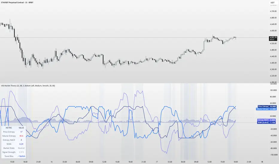
Information Theory Market AnalysisINFORMATION THEORY MARKET ANALYSIS
OVERVIEW
This indicator applies mathematical concepts from information theory to analyze market behavior, measuring the randomness and predictability of price and volume movements through entropy calculations. Unlike traditional technical indicators, it provides insight into market structure and regime changes.
KEY COMPONENTS
Four Main Signals:
• Price Entropy (Deep Blue): Measures randomness in price movements
• Volume Entropy (Bright Blue): Analyzes volume pattern predictability
• Entropy MACD (Purple): Shows relationship between price and volume entropy
• SEMM (Royal Blue): Stochastic Entropy Market Monitor - overall market randomness gauge
Market State Detection:
The indicator identifies seven distinct market states:
• Strong Trending (SEMM < 0.1)
• Weak Trending (0.1-0.2)
• Neutral (0.2-0.3)
• Moderate Random (0.3-0.5)
• High Randomness (0.5-0.8)
• Very Random (0.8-1.0)
• Chaotic (>1.0)
KEY FEATURES
Advanced Analytics:
• Signal Strength Confluence: 0-5 scale measuring alignment of multiple factors
• Entropy Crossovers: Detects shifts between accumulation and distribution phases
• Extreme Readings: Identifies statistical outliers for potential reversals
• Trend Bias Analysis: Directional momentum assessment
Information Dashboard:
• Real-time entropy values and market state
• Signal strength indicator with visual highlighting
• Trend bias with directional arrows
• Color-coded alerts for extreme conditions
Customizable Display:
• Adjustable SEMM scaling (5x to 100x) for optimal visibility
• Multiple line styles: Smooth, Stepped, Dotted
• 9 table positions with 3 size options
• Professional blue color scheme with transparency controls
Comprehensive Alert System - 15 Alert Types Including:
• Extreme entropy readings (price/volume)
• Crossover signals (dominance shifts)
• Market state changes (trending ↔ random)
• High confluence signals (3+ factors aligned)
HOW TO USE
Reading the Signals:
• Entropy Values > ±25: Strong structural signals
• Entropy Values > ±40: Extreme readings, potential reversals
• SEMM < 0.2: Trending market favors directional strategies
• SEMM > 0.5: Random market favors range/scalping strategies
Signal Confluence:
Look for multiple factors aligning:
• Signal Strength ≥ 3.0 for higher probability setups
• Background highlighting indicates confluence
• Table shows real-time strength assessment
Timeframe Optimization:
• Short-term (1m-15m): Entropy Length 14-22, Sensitivity 3-5
• Swing Trading (1H-4H): Default settings optimal
• Position Trading (Daily+): Entropy Length 34-55, Sensitivity 8-12
EDUCATIONAL APPLICATIONS
Market Structure Analysis:
• Understand when markets are trending vs. ranging
• Identify accumulation and distribution phases
• Recognize extreme market conditions
• Measure information content in price movements
Information Theory Concepts:
• Binary entropy calculations applied to financial data
• Probability distribution analysis of returns
• Statistical ranking and percentile analysis
• Momentum-adjusted randomness measurement
TECHNICAL DETAILS
Calculations:
• Uses binary entropy formula: -
• Percentile ranking across multiple timeframes
• Volume-weighted probability distributions
• RSI-adjusted momentum entropy (SEMM)
Customization Options:
• Entropy Length: 5-100 bars (default: 22)
• Average Length: 10-200 bars (default: 88)
• Sensitivity: 1.0-20.0 (default: 5.0, lower = more sensitive)
• SEMM Scaling: 5.0-100.0x (default: 30.0)
IMPORTANT NOTES
Risk Considerations:
• Indicator measures probabilities, not certainties
• High SEMM values (>0.5) suggest increased market randomness
• Extreme readings may persist longer than expected
• Always combine with proper risk management
Educational Purpose:
This indicator is designed for:
• Market structure analysis and education
• Understanding information theory applications in finance
• Developing probabilistic thinking about markets
• Research and analytical purposes
Performance Tips:
• Allow 200+ bars for proper initialization
• Adjust scaling and transparency for optimal visibility
• Use confluence signals for higher probability analysis
• Consider multiple timeframes for comprehensive analysis
DISCLAIMER
This indicator is for educational and analytical purposes. It does not constitute financial advice. Past performance does not guarantee future results. Always conduct your own research and consider your risk tolerance before making trading decisions.
Version: 5.0
Category: Oscillators, Volume, Market Structure
Best For: All timeframes, trending and ranging markets
Complexity: Intermediate to Advanced
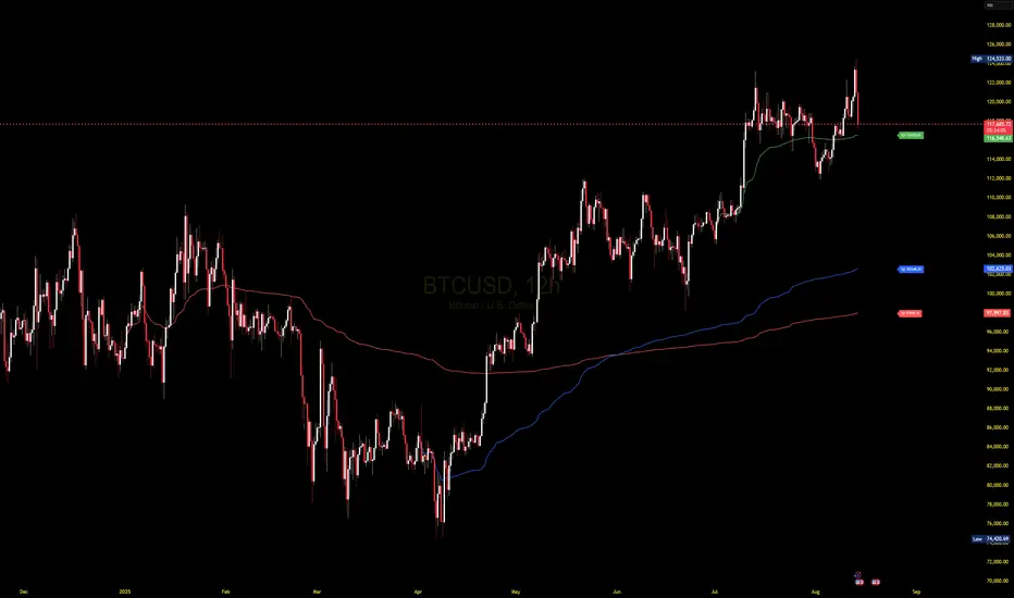
ATR-Scaled Deviation OscillatorATR-DevOsc is a custom momentum-and-volatility adaptive oscillator that scales N-bar price momentum by its rolling deviation and then reacts dynamically to sudden ATR spikes. By shrinking the deviation window when true volatility surges, it amplifies extreme moves—making medium-term trend shifts and deep drawdowns far more likely to breach your predefined thresholds.
Key features include:
• configurable momentum length and separate deviation length for precise control over look-back periods
• ATR Reaction Multiplier to tune how strongly sudden volatility spikes contract the deviation, boosting oscillator amplitude during extreme moves
• independent upper and lower threshold inputs for clear long/short signal definitions
• integrated candle-coloring overlay to immediately visualize trend state on your price chart
• built-in alert conditions for both oscillator-threshold crossovers and ATR-reactive triggers
This indicator is particularly useful for swing traders seeking medium-term entry and exit points in highly volatile markets like BTC. It combines normalized momentum readings with true volatility feedback, so large drawdowns or breakouts generate unmistakable signal events while routine noise stays filtered.
Note: ATR-DevOsc is provided “as is” without formal robustness or optimization testing. Past performance is not indicative of future results; use in live trading only after sufficient back-testing and validation.
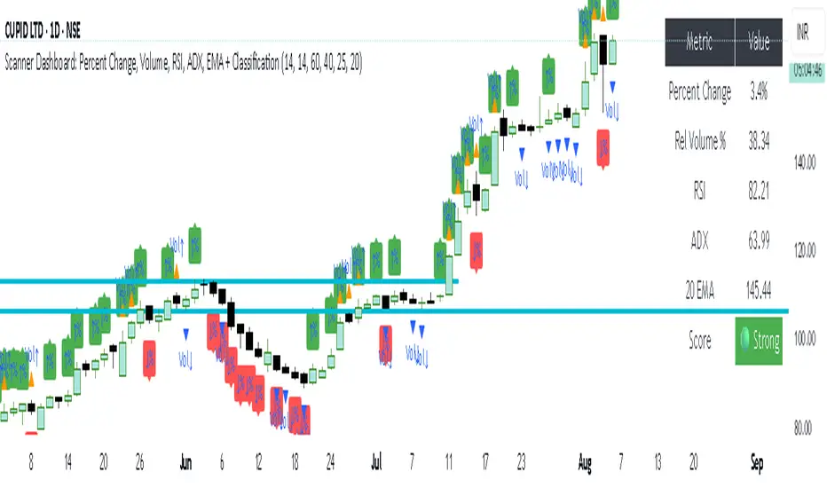
simple trend Scanner Dashboard Script Does
- Calculates key metrics:
- Percent Change from previous day
- Relative Volume (% vs 10-bar average)
- RSI and ADX for strength/trend
- 20 EMA for dynamic support/resistance
- Classifies market condition:
- 🟢 Strong if RSI > 60 and ADX > 25
- 🔴 Weak if RSI < 40 and ADX < 20
- ⚪ Neutral otherwise
- Displays a table dashboard:
- Compact, color-coded summary of all metrics
- Easy to scan visually
- Plots visual signals:
- Arrows and triangles for percent change and volume spikes
- Data window plots for deeper inspection
Crypto Options Greeks & Volatility Analyzer [BackQuant]Crypto Options Greeks & Volatility Analyzer
Overview
The Crypto Options Greeks & Volatility Analyzer is a comprehensive analytical tool that calculates Black-Scholes option Greeks up to the third order for Bitcoin and Ethereum options. It integrates implied volatility data from VOLMEX indices and provides multiple visualization layers for options risk analysis.
Quick Introduction to Options Trading
Options are financial derivatives that give the holder the right, but not the obligation, to buy or sell an underlying asset at a predetermined price (strike price) within a specific time period (expiration date). Understanding options requires grasping two fundamental concepts:
Call Options : Give the right to buy the underlying asset at the strike price. Calls increase in value when the underlying price rises above the strike price.
Put Options : Give the right to sell the underlying asset at the strike price. Puts increase in value when the underlying price falls below the strike price.
The Language of Options: Greeks
Options traders use "Greeks" - mathematical measures that describe how an option's price changes in response to various factors:
Delta : How much the option price moves for each $1 change in the underlying
Gamma : How fast delta changes as the underlying moves
Theta : Daily time decay - how much value erodes each day
Vega : Sensitivity to implied volatility changes
Rho : Sensitivity to interest rate changes
These Greeks are essential for understanding risk. Just as a pilot needs instruments to fly safely, options traders need Greeks to navigate market conditions and manage positions effectively.
Why Volatility Matters
Implied volatility (IV) represents the market's expectation of future price movement. High IV means:
Options are more expensive (higher premiums)
Market expects larger price swings
Better for option sellers
Low IV means:
Options are cheaper
Market expects smaller moves
Better for option buyers
This indicator helps you visualize and quantify these critical concepts in real-time.
Back to the Indicator
Key Features & Components
1. Complete Greeks Calculations
The indicator computes all standard Greeks using the Black-Scholes-Merton model adapted for cryptocurrency markets:
First Order Greeks:
Delta (Δ) : Measures the rate of change of option price with respect to underlying price movement. Ranges from 0 to 1 for calls and -1 to 0 for puts.
Vega (ν) : Sensitivity to implied volatility changes, expressed as price change per 1% change in IV.
Theta (Θ) : Time decay measured in dollars per day, showing how much value erodes with each passing day.
Rho (ρ) : Interest rate sensitivity, measuring price change per 1% change in risk-free rate.
Second Order Greeks:
Gamma (Γ) : Rate of change of delta with respect to underlying price, indicating how quickly delta will change.
Vanna : Cross-derivative measuring delta's sensitivity to volatility changes and vega's sensitivity to price changes.
Charm : Delta decay over time, showing how delta changes as expiration approaches.
Vomma (Volga) : Vega's sensitivity to volatility changes, important for volatility trading strategies.
Third Order Greeks:
Speed : Rate of change of gamma with respect to underlying price (∂Γ/∂S).
Zomma : Gamma's sensitivity to volatility changes (∂Γ/∂σ).
Color : Gamma decay over time (∂Γ/∂T).
Ultima : Third-order volatility sensitivity (∂²ν/∂σ²).
2. Implied Volatility Analysis
The indicator includes a sophisticated IV ranking system that analyzes current implied volatility relative to its recent history:
IV Rank : Percentile ranking of current IV within its 30-day range (0-100%)
IV Percentile : Percentage of days in the lookback period where IV was lower than current
IV Regime Classification : Very Low, Low, High, or Very High
Color-Coded Headers : Visual indication of volatility regime in the Greeks table
Trading regime suggestions based on IV rank:
IV Rank > 75%: "Favor selling options" (high premium environment)
IV Rank 50-75%: "Neutral / Sell spreads"
IV Rank 25-50%: "Neutral / Buy spreads"
IV Rank < 25%: "Favor buying options" (low premium environment)
3. Gamma Zones Visualization
Gamma zones display horizontal price levels where gamma exposure is highest:
Purple horizontal lines indicate gamma concentration areas
Opacity scaling : Darker shading represents higher gamma values
Percentage labels : Shows gamma intensity relative to ATM gamma
Customizable zones : 3-10 price levels can be analyzed
These zones are critical for understanding:
Pin risk around expiration
Potential for explosive price movements
Optimal strike selection for gamma trading
Market maker hedging flows
4. Probability Cones (Expected Move)
The probability cones project expected price ranges based on current implied volatility:
1 Standard Deviation (68% probability) : Shown with dashed green/red lines
2 Standard Deviations (95% probability) : Shown with dotted green/red lines
Time-scaled projection : Cones widen as expiration approaches
Lognormal distribution : Accounts for positive skew in asset prices
Applications:
Strike selection for credit spreads
Identifying high-probability profit zones
Setting realistic price targets
Risk management for undefined risk strategies
5. Breakeven Analysis
The indicator plots key price levels for options positions:
White line : Strike price
Green line : Call breakeven (Strike + Premium)
Red line : Put breakeven (Strike - Premium)
These levels update dynamically as option premiums change with market conditions.
6. Payoff Structure Visualization
Optional P&L labels display profit/loss at expiration for various price levels:
Shows P&L at -2 sigma, -1 sigma, ATM, +1 sigma, and +2 sigma price levels
Separate calculations for calls and puts
Helps visualize option payoff diagrams directly on the chart
Updates based on current option premiums
Configuration Options
Calculation Parameters
Asset Selection : BTC or ETH (limited by VOLMEX IV data availability)
Expiry Options : 1D, 7D, 14D, 30D, 60D, 90D, 180D
Strike Mode : ATM (uses current spot) or Custom (manual strike input)
Risk-Free Rate : Adjustable annual rate for discounting calculations
Display Settings
Greeks Display : Toggle first, second, and third-order Greeks independently
Visual Elements : Enable/disable probability cones, gamma zones, P&L labels
Table Customization : Position (6 options) and text size (4 sizes)
Price Levels : Show/hide strike and breakeven lines
Technical Implementation
Data Sources
Spot Prices : INDEX:BTCUSD and INDEX:ETHUSD for underlying prices
Implied Volatility : VOLMEX:BVIV (Bitcoin) and VOLMEX:EVIV (Ethereum) indices
Real-Time Updates : All calculations update with each price tick
Mathematical Framework
The indicator implements the full Black-Scholes-Merton model:
Standard normal distribution approximations using Abramowitz and Stegun method
Proper annualization factors (365-day year)
Continuous compounding for interest rate calculations
Lognormal price distribution assumptions
Alert Conditions
Four categories of automated alerts:
Price-Based : Underlying crossing strike price
Gamma-Based : 50% surge detection for explosive moves
Moneyness : Deep ITM alerts when |delta| > 0.9
Time/Volatility : Near expiration and vega spike warnings
Practical Applications
For Options Traders
Monitor all Greeks in real-time for active positions
Identify optimal entry/exit points using IV rank
Visualize risk through probability cones and gamma zones
Track time decay and plan rolls
For Volatility Traders
Compare IV across different expiries
Identify mean reversion opportunities
Monitor vega exposure across strikes
Track higher-order volatility sensitivities
Conclusion
The Crypto Options Greeks & Volatility Analyzer transforms complex mathematical models into actionable visual insights. By combining institutional-grade Greeks calculations with intuitive overlays like probability cones and gamma zones, it bridges the gap between theoretical options knowledge and practical trading application.
Whether you're:
A directional trader using options for leverage
A volatility trader capturing IV mean reversion
A hedger managing portfolio risk
Or simply learning about options mechanics
This tool provides the quantitative foundation needed for informed decision-making in cryptocurrency options markets.
Remember that options trading involves substantial risk and complexity. The Greeks and visualizations provided by this indicator are tools for analysis - they should be combined with proper risk management, position sizing, and a thorough understanding of options strategies.
As crypto options markets continue to mature and grow, having professional-grade analytics becomes increasingly important. This indicator ensures you're equipped with the same analytical capabilities used by institutional traders, adapted specifically for the unique characteristics of 24/7 cryptocurrency markets.

DeltaTrace ForecastDeltaTrace Forecast is a forward-looking projection tool that visualizes the probable directional path of price using a multi-timeframe momentum model rooted in volatility-adjusted nonlinear dynamics. Rather than relying on traditional indicators that react to price after the fact, DeltaTrace estimates future price motion by tracing the progression of momentum changes across expanding timeframes—then scaling those deltas using adaptive volatility to forecast a plausible path forward.
At its core, DeltaTrace constructs a momentum vector from a series of smoothed z-scores derived from increasing multiples of the current chart's timeframe. These z-scores are normalized using a hyperbolic tangent function (tanh), which compresses extreme values and emphasizes meaningful deviations without being overly sensitive to outliers. This nonlinear normalization ensures that explosive moves are weighted with less distortion, while still preserving the shape and direction of the underlying trend.
Once the z-scores are calculated for a range of 12 timeframes (from 1× the current timeframe up to 12×), the indicator computes the first difference between each adjacent pair. These differences—or deltas—represent the change in momentum from one timeframe to the next. In this structure, a strong positive delta implies momentum is strengthening as we look into higher timeframes, while a negative delta reflects waning or reversing strength.
However, not all deltas are treated equally. To make the projection adaptive to market volatility and temporally meaningful, each delta is scaled by the square root of its corresponding timeframe multiple, weighted by the ATR (Average True Range) of the base timeframe. This square-root volatility scaling mirrors the behavior of Brownian motion and reflects the natural geometric diffusion of price over time. By applying this scaling, the model tempers its forecast according to recent volatility while maintaining proportional distance over longer time horizons.
The result is a chain of projected price steps—11 in total—starting from the current closing price. These steps are cumulative, meaning each one builds upon the previous, forming a continuously adjusted polyline that represents the most recent forecast path of price. Each point in the forecast line is directional: if the next projected point is above the last, the segment is colored green (upward momentum); if below, it is colored red (downward momentum). This color coding gives immediate visual feedback on the nature of the projected path and allows for intuitive at-a-glance interpretation.
What makes DeltaTrace unique is its combination of ideas from signal processing, time-series momentum analysis, and volatility theory. Instead of relying on static support/resistance levels or lagging moving averages, it dynamically adapts to both momentum curvature and volatility structure. This allows it to be used not just for trend confirmation, but also for top-down bias fading, reversal anticipation, and path-following strategies.
Traders can use DeltaTrace in a variety of ways depending on their style:
For trend traders, a consistent upward or downward curve in the forecast suggests directional continuation and can be used for position sizing or confirmation of bias.
For mean-reversion traders, exaggerated divergence between the current price and the first few forecast points may indicate temporary exhaustion or overextension.
For scalpers or intraday traders, the short-term bend or flattening of the initial segments can reveal early signs of weakening momentum or build-up before breakout.
For swing traders, the full shape of the polyline gives an evolving map of market rhythm across time compression, allowing for context-aware decision-making.
It’s important to understand that this is a path projection tool, not a precise price target predictor. The forecast does not attempt to predict exact price levels at exact bars, but rather illustrates how the market might evolve if the current multi-timeframe momentum structure persists. Like all models, it should be interpreted probabilistically and used in conjunction with other confirmation signals, risk management tools, or strategy frameworks.
Inputs allow customization of the z-score calculation length and ATR window to tune the sensitivity of the model. The color scheme for up/down forecast segments can also be adjusted for personal preference. Additionally, users can toggle the polyline forecast on or off, which may be useful for pairing this indicator with others in a crowded chart layout.
Because the forecast path is calculated only on the last bar, it does not repaint or shift once the candle closes—preserving historical accuracy for visual inspection and backtesting reference. However, it is also sensitive to changes in volatility and momentum structure, meaning it updates each bar as conditions evolve, making it most effective in real-time decision support.
DeltaTrace Forecast is particularly well-suited for traders who want a deeper understanding of hidden momentum shifts across timeframes without relying on traditional trend-following tools. It reveals the shape of future possibility based on present dynamics, offering a compact yet powerful visualization of directional bias, transition risk, and path strength.
To maximize its utility, consider pairing DeltaTrace with volume profiles, order flow tools, higher timeframe zones, or market structure indicators. Used in context, it becomes a powerful companion to both systematic and discretionary trading styles—especially for those who appreciate a blend of mathematics and intuition in their market analysis.
This indicator is not based on magic or black-box logic; every component—from the z-score standardization to the volatility-adjusted deltas—is fully transparent and grounded in simple, interpretable mechanics. If you're looking for a reliable way to visualize multi-timeframe bias and momentum diffusion, DeltaTrace provides a unique lens through which to interpret future potential in an ever-shifting market landscape.

ZigZag Volume Profile [ChartPrime]⯁ OVERVIEW
ZigZag Volume Profile combines swing structure with volume analytics by plotting a ZigZag of major price swings and overlaying a detailed volume profile around each swing. At the end of each swing, it highlights the Point of Control (POC) — the price level with the highest traded volume — and extends it forward to identify key areas of potential support or resistance.
⯁ KEY FEATURES
ZigZag Swing Detection:
Automatically detects swing highs and lows based on a user-defined length, creating clean visual segments of market structure.
These segments act as boundaries for volume profile calculations.
swingHigh = ta.highest(swingLength)
swingLow = ta.lowest(swingLength)
ZigZag Channel Visualization:
The ZigZag structure is connected with sloped lines, forming a visual “channel” of the price movement.
The ZigZag can optionally, scaled by ATR.
Volume Profile Around Each Swing:
For every completed swing (high to low or low to high), the indicator constructs a full volume profile using user-defined bin counts.
It scans volume across price levels in the swing and plots histogram-style bins using a gradient color to indicate volume magnitude.
Dynamic Bin Width and Slope Adjustment:
Bins are distributed across a vertical ATR-based range, and their width is adjusted based on the percentage of total swing volume.
The volume fill direction is adapted to the swing’s slope for visually aligned plotting.
POC Detection and Extension:
The highest volume bin in each swing is identified as the Point of Control (POC).
This level is plotted with a thicker line and extended horizontally into the future as a key reaction level.
Automatic POC Expiry on Price Interaction:
POC lines are continuously extended unless breached by price.
When price crosses the POC level, the extension is terminated — signaling that the level may have been absorbed.
Clean Volume Bin Visualization:
Bin colors range from green (low volume) to blue (higher volume), with the POC always marked in red by default for easy identification.
Volume percentages are optionally labeled at each bin level.
Flexible Swing Profile Parameters:
Users can control:
Number of volume bins
Bin width
Channel width (ATR factor)
Visibility of the swing channel or POC lines
Efficient Memory Handling:
Old POC lines and volume profiles are automatically removed from memory after a threshold to keep charts clean and performant.
⯁ USAGE
Use ZigZag swings to define market structure visually.
Analyze volume profile around each swing to understand where most trading activity occurred.
Use POC extensions as dynamic support/resistance zones for entries, stops, or take-profits.
Watch for price interaction with extended POC lines — breaks may suggest absorbed liquidity or breakout potential.
Use the ATR-based channel width to adapt profiles based on market volatility.
⯁ CONCLUSION
ZigZag Volume Profile offers a powerful fusion of structure and volume. By plotting detailed volume profiles over each price swing and extending the POC as actionable S/R levels, this tool provides deep insight into market participation zones — giving traders a tactical edge in both ranging and trending environments.
Fisher Crossover StrategyThe Fisher Crossover Strategy is a popular technical trading method that uses the Fisher Transform indicator developed by John Ehlers. This indicator mathematically converts price data into a normal Gaussian distribution, making market turning points sharper and easier to identify. The strategy is based on two lines: the Fisher line, which is the main transformed price value, and the Trigger line, which is a one-period lag of the Fisher line. Traders use the crossover of these lines to determine buy and sell opportunities.
A buy signal is generated when the Fisher line crosses above the Trigger line, indicating that bullish momentum may be starting, while a sell signal occurs when the Fisher line crosses below the Trigger line, suggesting a possible bearish reversal. Signals that occur relative to the zero line are often considered stronger; for example, a buy signal below the zero line may indicate a deeper market reversal. The strategy is simple to follow and can be applied to various markets including stocks, forex, commodities, and cryptocurrencies.
However, like all crossover strategies, it can produce false signals during sideways or ranging markets. To reduce whipsaws, traders often combine the Fisher Crossover Strategy with other tools such as support and resistance levels, volume analysis, or moving averages. Proper risk management with stop-loss and take-profit levels is also essential. Overall, the Fisher Crossover Strategy is valued for its clear entry and exit rules and its ability to highlight potential market reversals earlier than many other indicators.
Volume Based Analysis V 1.00
Volume Based Analysis V1.00 – Multi-Scenario Buyer/Seller Power & Volume Pressure Indicator
Description:
1. Overview
The Volume Based Analysis V1.00 indicator is a comprehensive tool for analyzing market dynamics using Buyer Power, Seller Power, and Volume Pressure scenarios. It detects 12 configurable scenarios combining volume-based calculations with price action to highlight potential bullish or bearish conditions.
When used in conjunction with other technical tools such as Ichimoku, Bollinger Bands, and trendline analysis, traders can gain a deeper and more reliable understanding of the market context surrounding each signal.
2. Key Features
12 Configurable Scenarios covering Buyer/Seller Power convergence, divergence, and dominance
Advanced Volume Pressure Analysis detecting when both buy/sell volumes exceed averages
Global Lookback System ensuring consistency across all calculations
Dominance Peak Module for identifying strongest buyer/seller dominance at structural pivots
Real-time Signal Statistics Table showing bullish/bearish counts and volume metrics
Fully customizable inputs (SMA lengths, multipliers, timeframes)
Visual chart markers (S01 to S12) for clear on-chart identification
3. Usage Guide
Enable/Disable Scenarios: Choose which signals to display based on your trading strategy
Fine-tune Parameters: Adjust SMA lengths, multipliers, and lookback periods to fit your market and timeframe
Timeframe Control: Use custom lower timeframes for refined up/down volume calculations
Combine with Other Indicators:
Ichimoku: Confirm volume-based bullish signals with cloud breakouts or trend confirmation
Bollinger Bands: Validate divergence/convergence signals with overbought/oversold zones
Trendlines: Spot high-probability signals at breakout or retest points
Signal Tables & Peaks: Read buy/sell volume dominance at a glance, and activate the Dominance Peak Module to highlight key turning points.
4. Example Scenarios & Suggested Images
Image #1 – S01 Bullish Convergence Above Zero
S01 activated, Buyer Power > 0, both buyer power slope & price slope positive, above-average buy volume. Show S01 ↑ marker below bar.
Image #2 – Combined with Ichimoku
Display a bullish scenario where price breaks above Ichimoku cloud while S01 or S09 bullish signal is active. Highlight both the volume-based marker and Ichimoku cloud breakout.
Image #3 – Combined with Bollinger Bands & Trendlines
Show a bearish S10 signal at the upper Bollinger Band near a descending trendline resistance. Highlight the confluence of the volume pressure signal with the band touch and trendline rejection.
Image #4 – Dominance Peak Module
Pivot low with green ▲ Bull Peak and pivot high with red ▼ Bear Peak, showing strong dominance counts.
Image #5 – Statistics Table in Action
Bottom-left table showing buy/sell volume, averages, and bullish/bearish counts during an active market phase.
5. Feedback & Collaboration
Your feedback and suggestions are welcome — they help improve and refine this system. If you discover interesting use cases or have ideas for new features, please share them in the script’s comments section on TradingView.
6. Disclaimer
This script is for educational purposes only. It is not financial advice. Past performance does not guarantee future results. Always do your own analysis before making trading decisions.
Tip: Use this tool alongside trend confirmation indicators for the most robust signal interpretation.
