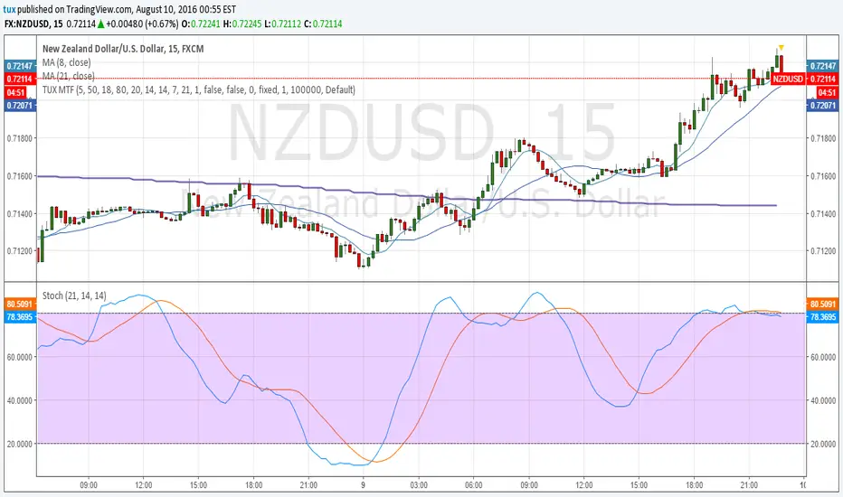
MULTIPLE TIME-FRAME STRATEGY(TREND, MOMENTUM, ENTRY) Hey everyone, this is one strategy that I have found profitable over time. It is a multiple time frame strategy that utilizes 3 time-frames. Highest time-frame is the trend, medium time-frame is the momentum and short time-frame is the entry point.
Long Term:
- If closed candle is above entry then we are looking for longs, otherwise we are looking for shorts
Medium Term:
- If Stoch SmoothK is above or below SmoothK and the momentum matches long term trend then we look for entries.
Short Term:
- If a moving average crossover(long)/crossunder(short) occurs then place a trade in the direction of the trend.
Close Trade:
- Trade is closed when the Medium term SmoothK Crosses under/above SmoothD.
You can mess with the settings to get the best Profit Factor / Percent Profit that matches your plan.
Best of luck!
Cerca negli script per "entry"
Reversal Entry on StdDev & ICT LevelsThis custom indicator combines Standard Deviation Channels with ICT Killzone session levels to identify high-probability reversal entries. It triggers long/short signals when:
Price extends beyond ±2 standard deviations (overbought/oversold conditions)
A reversal wick (e.g., pin bar or hammer) confirms exhaustion
Price bounces off a key session level (e.g., NYAM high or low)
The tool visually plots deviation bands and session ranges, helping traders identify smart entry points aligned with market structure and time-based liquidity zones. Suitable for scalpers and intraday traders using ICT concepts.

NFO Rolling Straddle with Entry ExitNFO Rolling Entry Exit based on combined premiums, use on Options chart as Underlying chart doesn't allow long history

Trend Entry Signal v2Used for entry signals. More efficient for scalp trades, at least 70% correct prediction, more efficent on stablecoins.

ETH 1-2-3 Rigor Strategy Entry & 2:1 Risk-Rewar- By: Labaxuria Descrição em Inglês (Copy & Paste):
This script is a technical analysis tool designed specifically for ETH/USDT on Daily (1D) and Weekly (1W) timeframes. It identifies the classic 1-2-3 reversal pattern to provide high-probability entry points with a strictly disciplined risk management approach.
Core Features:
C3 Trigger Identification: The indicator highlights the "Candle 3" (Confirmation Candle) where the breakout of "Point 2" occurs, validating the market structure shift.
Automated 2:1 Risk-Reward: Upon a BUY or SELL signal, the script automatically plots a Red Line (Stop Loss) at the recent pivot and a Green Line (Take Profit) at a fixed 2:1 ratio. This ensures that every win is twice the size of a potential loss.
Trend Filtering (Gray Line): It includes a 20-period Moving Average to ensure trades are aligned with the prevailing market momentum.
Compression Detection (White Candles): Identifies "Inside Bars" by coloring the candle body or borders white. This warns the trader of price compression and potential volatility buildup before a breakout.
How to Use:
BUY + C3: Enter long when the price closes above Point 2, ideally while trading above the gray 20-SMA.
SELL + C3: Enter short when the price closes below Point 2, ideally while trading below the gray 20-SMA.
Exit Strategy: Follow the plotted levels strictly. Exit at the red line to protect capital or at the green line to book profits.

The Strat: 3-2D Setup Label + Entry, Target & AlertsThis is an indicator that identifies the 3-2D setup based on TheStrat & will alert you if you have this on the chart. Once the 3-2D setup happens this will give you the entry, target and price labels. You can change the font size, label colors and add optional alerts.

Sniper Entry AU - AYUSHThis indicator combines EMA 9, EMA 15, and VWAP to identify trend direction and intraday strength. EMA 9 and EMA 15 show short-term momentum and crossover signals, while VWAP acts as an institutional reference point for fair value. Together, they help traders spot trend continuation, pullbacks, and high-quality entry zones during intraday sessions.


Renko 2-block entry, 1-block exit (signals EVERY block)Renko 2-block entry, 1-block exit (signals EVERY block)

CM_MACD_Ult_MTF + Entry SignalsThis script is an enhanced and updated version of the classic CM_Ult_MacD_MTF originally created by ChrisMoody.
It preserves the full functionality, look, and behavior of the original multi-timeframe MACD, including:
Multi-timeframe MACD calculation
4-color histogram based on momentum direction
Optional MACD and Signal line display
Optional crossover dots
Color-changing MACD line on signal cross
Zero-line reference
This upgraded version adds entry signals based on MACD/Signal crossovers:
New Features Added
LONG @ price label when MACD crosses above Signal
SHORT @ price label when MACD crosses below Signal
Labels appear directly at the crossover point
Full support for Pine Script® v6, making it compatible with TradingView’s latest publishing requirements
Why this version?
The original script was written in an older Pine version and was no longer publishable.
This version keeps the full visual identity and logic of the classic MACD while adding modern compatibility and helpful trading signals.
Credits
Original concept and visual framework: ChrisMoody
Added features, Pine v6 migration, and enhancements: tgambinox

Positional Supertrend Strategy (1D Filter + 2H Entry)Positional Supertrend Strategy (1D Filter + 2H Entry)

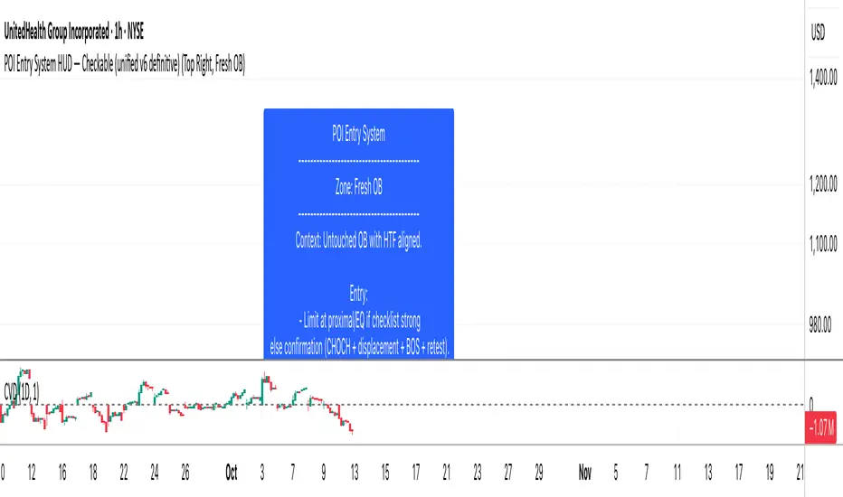
Order Block Smart Entry (v6)very useful indicator, analyze multiframes to identify the trend, then find out the valid order block and after analyzing lower time frame entry gives the singal.

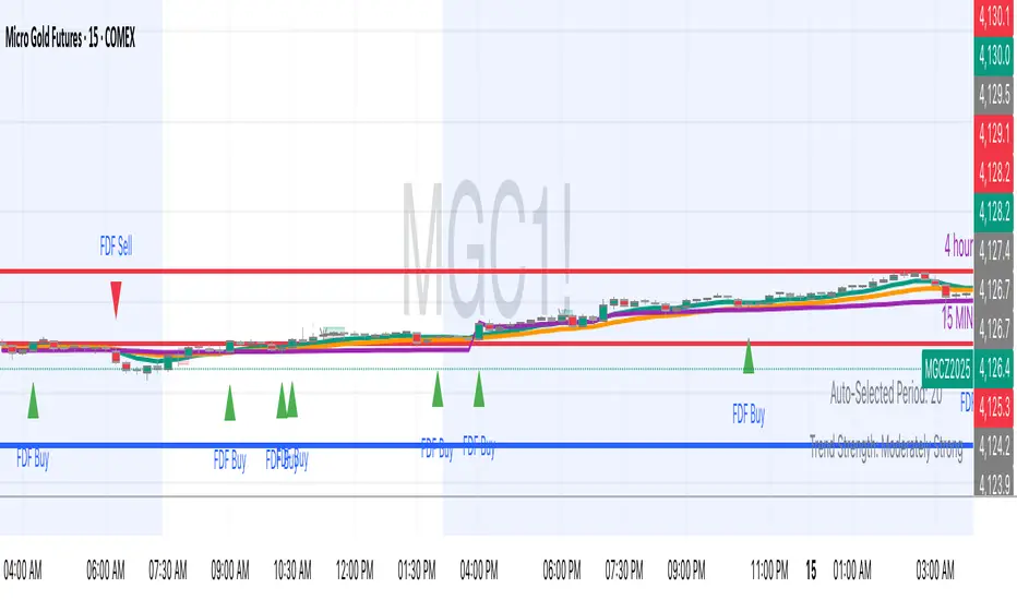
FDF — EMAs+VWAP with setup & entry (stable scale)the 9 and 21, vwap - and support an restianst, marking each entry when it pulling in our out to the 21. used 90% of the candle over the 21
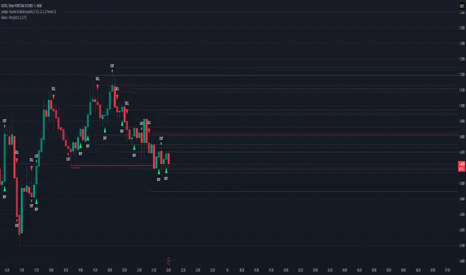
Magracia Entry-Exit 5 Min Time frame//------------------------------------------------------------------------------------------------------
// 🧭 Indicator Description
//------------------------------------------------------------------------------------------------------
// 📘 Overview:
// This indicator is a modified version of the LuxAlgo pattern logic designed to detect
// high-probability **RBD (Rally–Base–Drop)** and **DBR (Drop–Base–Rally)** reversal structures
// directly on the current candle. It automatically identifies potential BUY and SELL zones,
// plots corresponding trade signals, and dynamically calculates **Take Profit (TP)** and **Stop Loss (SL)** levels.
//
// The goal of this tool is to give clear, visually guided trade entries and exits that
// follow price structure and momentum changes without repainting historical data.
//
//------------------------------------------------------------------------------------------------------
// 🧩 How It Works:
// • **RBD (Rally–Base–Drop)** → Indicates a bearish reversal (SELL signal)
// • **DBR (Drop–Base–Rally)** → Indicates a bullish reversal (BUY signal)
// • Optional **RBR / DBD** continuation patterns can be toggled on for trend continuation setups.
// • When a signal is detected, the script automatically places:
// ▫ A BUY or SELL marker at the candle
// ▫ Dynamic TP (green dotted line) and SL (red dotted line) levels
// ▫ An EXIT marker when either TP or SL is reached
//
//------------------------------------------------------------------------------------------------------
// ⚙️ Inputs:
// • Enable or disable individual pattern types (RBD, RBR, DBD, DBR)
// • Toggle continuation patterns (RBR/DBD)
// • Customize Take Profit and Stop Loss percentages
// • Adjust rally/drop bar colors for easier pattern visualization
//
//------------------------------------------------------------------------------------------------------
// 🧠 Usage Tips:
// • Works best on volatile pairs and short–term timeframes (1m to 15m)
// • Can be combined with volume or trend filters for stronger confirmation
// • When used on higher timeframes (e.g., 4H+), increase TP/SL percentage range
//
//------------------------------------------------------------------------------------------------------
// ⚠️ Notes:
// • Signals are plotted **in real-time on the current candle** (not delayed).
// • This indicator is for visual and educational use only and does not guarantee profitability.
// • For optimal results, combine it with proper risk management and confirmation indicators.
//
//------------------------------------------------------------------------------------------------------
// © Gideon (CC BY-NC-SA 4.0 Licensed)
//------------------------------------------------------------------------------------------------------
ARGT Possible entry and exit points:This is just an observation, and not any type of financial advice.
]To identify key entry and exit points. In addition, this is based on YTD and yearly charts. This is a work in progress.

EMA + MACD Entry Signals (Jason Wang)EMA9、20、200 + MACD(12、26、9) Entry Signals ,严格的设置出入场条件
1.做多的k棒:
• EMA9 > EMA200
• EMA20 > EMA200
• EMA9 > EMA20
• MACD DIF > 0 且 DIF > DEM
• 入场信号:
• DIF 上穿 DEM
• 或 EMA9 上穿 EMA20
2.做空的k棒:
• EMA9 < EMA200
• EMA20 < EMA200
• EMA9 < EMA20
• MACD DIF < 0 且 DIF < DEM
• 入场信号:
• DIF 下穿 DEM
• 或 EMA9 下穿 EMA20

Multi Asset Position Size Calculator (Extended with Entry ModeMulti Asset Position Size Calculator (Extended with Entry Mode

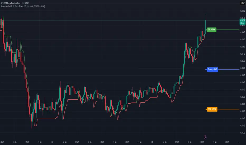
Supertrend with TP, Entry & DCAThis script is super trend plus, horizontal lines for Take Profit, Entry Price and DCA.
EMA Pullback Entry SignalsEMA Pullback Entry Signals is a tool designed to help traders identify trend continuation opportunities by detecting price pullbacks toward a slow EMA (Exponential Moving Average) during trending conditions.
This indicator combines moving average crossovers, price interaction with EMAs, and optional filtering to improve the timing and quality of trend entries.
Core Features:
Golden Cross / Death Cross Detection
Golden Cross: Fast EMA crossing above Slow EMA
Death Cross: Fast EMA crossing below Slow EMA
Optional X-shaped markers for crossover visualization
Pullback Signal on Slow EMA
Green triangle: Price crosses up through the slow EMA during a bullish trend
Red triangle: Price crosses down through the slow EMA during a bearish trend
Designed to capture continuation entries after a trend pullback
Optional Fast EMA Signals
Green arrow: Price crosses above fast EMA in a bull trend
Red arrow: Price crosses below fast EMA in a bear trend
Helps confirm minor retracements or short-term momentum shifts
Sideways Market Filter
Suppresses signals when the fast and slow EMAs are too close
Prevents entries during low-trend or choppy price action
Cooldown Timer
Enforces a minimum bar interval between signals to reduce overtrading
Helps avoid multiple entries from clustered signals
Custom Alerts
Alerts available for all signal types
Include ticker and timeframe in each alert message
Configurable Settings:
Fast and slow EMA lengths1
Toggle individual signal types (pullbacks, fast EMA crosses, crossovers)
Enable/disable cooldown logic and set bar duration
Sideways market detection sensitivity (EMA proximity threshold)
Primary Use Case
This script is most useful for trend-following traders seeking to enter pullbacks after a trend is established. When the price retraces to the slow EMA and then resumes in the trend direction, it can offer high-quality continuation setups. Works well across timeframes and markets.

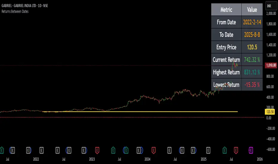
Returns Since Entry DateThis indicator shows the returns and max returns since entry date in a nice tabular format.
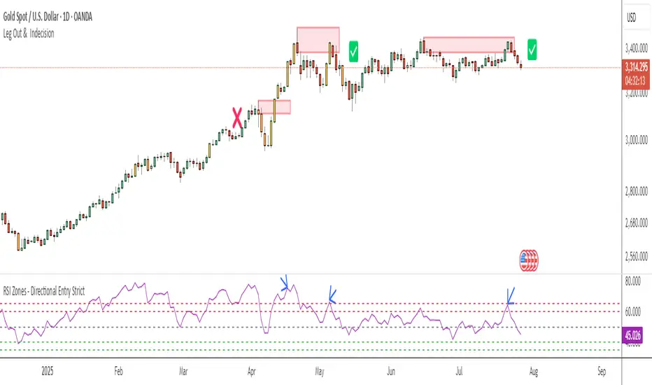
RSI Zones - Directional Entry Strict RSI Zones – Directional Entry Tool (Modified RSI)
This is a simple modification of the standard RSI indicator. I’ve added two custom horizontal lines at the 60–65 and 35–40 zones to help spot momentum shifts and potential reversal points.
60–65 zone: When RSI returns here from above 65, it often signals weakening bullish momentum — useful for spotting short opportunities.
35–40 zone: When RSI returns here from below 35, it can indicate momentum loss on the downside — good for potential long setups.
This version helps traders filter out weak signals and avoid chasing extreme moves.
It works best when combined with price action, structure, or divergence.
Only 2 lines were added to the default RSI for better zone awareness. Everything else remains unchanged.
Stop Order Entry with Filters and Line📌 名称: Stop Order Entry with Filters (挂单入场辅助工具)
🧠 作者: Kuixi Zhu
🛠️ 功能简介:
本指标用于识别高质量的 Bull/Bear bar,并在其上方(或下方)自动绘制挂单入场线,帮助你基于 Price Action 策略设置 **buy stop / sell stop** 挂单。
✅ 特性:
- Bull bar:收盘靠近 high,且 bar 波动大于平均(ABR) → 在 high+1tick 画绿线(buy stop)
- Bear bar:收盘靠近 low,且 bar 波动大于平均 → 在 low-1tick 画红线(sell stop)
- 支持自定义线条长度、ABR周期、强度过滤标准
🔍 核心逻辑:
- `(close - low) / (high - low)` 衡量收盘靠近 high 的程度
- `barRange > avg(barRange)` 控制有效波动性
- 使用 `line.new` 动态画出可视化入场价格
📊 应用场景:
- 趋势交易中的顺势挂单策略
- price action 高质量 bar 的识别辅助
- 多头突破、空头反转结构的自动提示
⚙️ 参数可调:
- 最低收盘位置比例(default: 0.9)
- 最小 bar 波动倍数(相对 ABR)
- 横线绘制长度(default: 5 bars)
---
