Persistence# Persistence
## What it does
Measures **price change persistence**, defined as the percentage of bars within a lookback window that closed higher than the prior close. A high value means the instrument has been closing up frequently, which can indicate durable momentum. This mirrors Stockbee’s idea: *select stocks with high price change persistence*, and then combine **momentum plus persistence**.
## Can be used for scanning in PineScreener
## Calculation
* `isUp` is true when `close > close `.
* `countUp` counts true instances over the last `len` bars.
* `pctUp = 100 * countUp / len`, bounded between 0 and 100.
* A 50% level is a natural baseline. Above 50% suggests more up closes than down closes in the window.
## Inputs
* **Lookback bars (`len`)**: default 252 for roughly one trading year on a daily chart. On weekly charts use something like 52, on monthly charts use 12.
## How to use
1. **Screen for persistence**
Sort a watchlist by the plotted value, higher is better. Many momentum traders start looking above 58 to 65 percent, then layer a trend filter.
2. **Combine with momentum**
Examples, pick tickers with:
* `pctUp > 60`, and price above a rising EMA50 or EMA100.
* `pctUp rising` and weekly ROC positive.
3. **Switch timeframe to change the horizon**
* Daily chart with `len = 252` approximates one year.
* Weekly chart with `len = 52` approximates one year.
* Monthly chart with `len = 12` approximates one year.
## TC2000 equivalence
Stockbee’s TC2000 expression:
```
CountTrue(c > c1, 252)
```
## Interpretation guide
* **70 to 90**: very strong persistence; often trend leaders, check for extensions and risk controls.
* **60 to 70**: constructive persistence; good hunting ground for swing setups that also pass momentum filters.
* **50**: neutral baseline; around random up vs down frequency.
* **Below 50**: persistent weakness; consider only for mean reversion or short strategies.
## Practical tips
* **Event effects**: ex-dividend gaps can reduce persistence on high yield names. Earnings gaps can swing the value sharply.
* **Survivorship bias**: when backtesting on curated lists, persistence can look cleaner than in live scans.
* **Liquidity**: thin names may show noisy persistence due to erratic prints.
## Reference to Stockbee
* “One way to select stocks for swing trading is to find those with high price change persistence.”
* “Persistence can be calculated on a daily, monthly, or weekly timeframe.”
* TC2000 function: `CountTrue(c > c1, 252)`
* Example noted in the tweet: CVNA had very high one-year price persistence at the time of that post.
* Takeaway: **look for momentum plus persistence**, not persistence alone.
Cerca negli script per "gaps"

Bitcoin cme gap indicators, BINANCE vs CME exchanges premium gap
# CME BTC Premium Indicator Documentation CME:BTC1!
## 1. Overview
Indicator Name: CME BTC Premium
Platform: TradingView (Pine Script v6)
Type: Premium / Gap Analysis
Purpose:
* Visualize the CME BTC futures premium/discount relative to Binance BTCUSDT spot price.
* Detect gap-up or gap-down events on the daily chart.
* Assess short-term market sentiment and potential volatility through price discrepancies.
## 2. Key Features
1. CME Premium Calculation
* Formula:
CME Premium(%) = ((CME Price - Binance Price) / Binance Price) X 100
* Positive premium: CME futures are higher than spot → Color: Blue
* Negative premium: CME futures are lower than spot → Color: Purple
2. Premium Visualization Options
* `Column` (default)
* `Line`
3. Daily Gap Detection (Daily Chart Only)
* Gap Up: CME open > previous high × 1.0001 (≥ 0.01%)
* Gap Down: CME open < previous low × 0.9999 (≤ 0.01%)
* Visualization:
* Bar Color:
* Gap Up → Yellow (semi-transparent)
* Gap Down → Blue (semi-transparent)
* Background Color:
* Gap Up → Yellow (semi-transparent)
* Gap Down → Blue (semi-transparent)
4. Label Display
* If `Show CME Label` is enabled, the last bar displays a premium percentage label.
* Label color matches premium color; text color: Black.
* Style: `style_label_upper_left`, Size: `small`.
## 3. User Inputs
| Option Name | Description | Type / Default |
| -------------- | ------------------------- | --------------------------------------- |
| Show CME Label | Display CME premium label | Boolean / true |
| CME Plot Type | CME premium chart style | String / Column (Options: Column, Line) |
## 4. Data Sources
| Data Item | Symbol | Description |
| ------------- | ---------------- | ----------------------------- |
| Binance Price | BINANCE\:BTCUSDT | Spot BTC price |
| CME Price | CME\:BTC1! | CME BTC futures closing price |
| CME Open | CME\:BTC1! | CME BTC futures open price |
| CME Low | CME\:BTC1! | CME BTC futures low price |
| CME High | CME\:BTC1! | CME BTC futures high price |
## 5. Chart Display
1. Premium Column/Line
* Displays the CME premium percentage in real-time.
* Color: Premium ≥ 0 → Blue, Premium < 0 → Purple
2. Zero Line
* Indicates CME futures are at parity with spot for quick visual reference.
3. Gap Highlight
* Applied only on daily charts.
* Gap-up or gap-down is highlighted using bar and background colors.
4. Label
* Shows the latest CME premium percentage for quick monitoring.
## 6. Use Cases
* Analyze spot-futures premium to gauge CME market sentiment.
* Identify short-term volatility and potential trend reversals through daily gaps.
* Combine premium and gap analysis to support altcoin trend analysis and position strategy.
## 7. Limitations
* This indicator does not provide investment advice or trading recommendations; it is for informational purposes only.
* Data delays, API restrictions, or exchange differences may result in calculation discrepancies.
* Gap detection is meaningful only on daily charts; other timeframes may not provide valid signals.

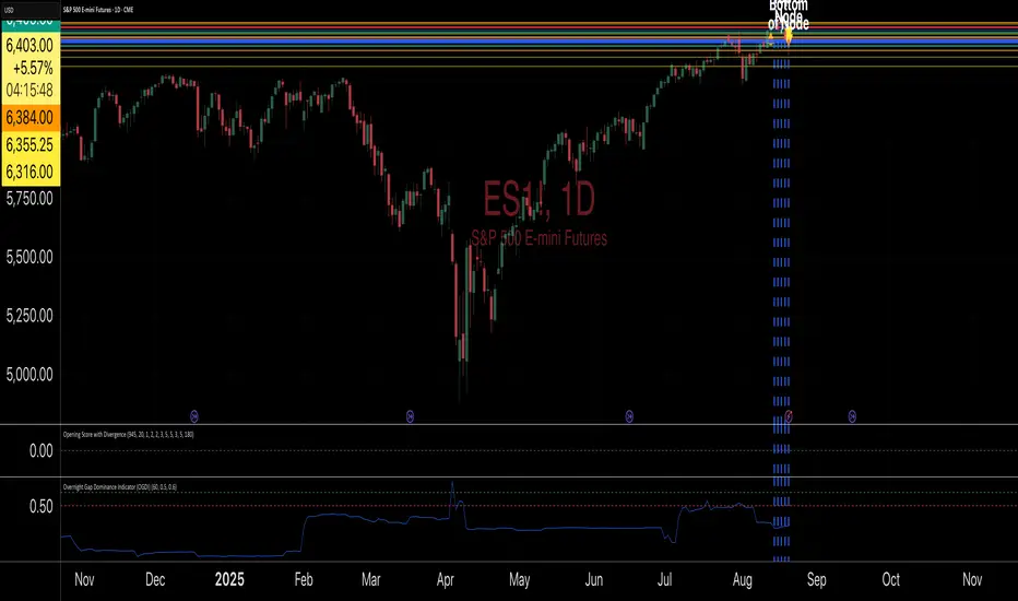
Overnight Gap Dominance Indicator (OGDI)The Overnight Gap Dominance Indicator (OGDI) measures the relative volatility of overnight price gaps versus intraday price movements for a given security, such as SPY or SPX. It uses a rolling standard deviation of absolute overnight percentage changes divided by the standard deviation of absolute intraday percentage changes over a customizable window. This helps traders identify periods where overnight gaps predominate, suggesting potential opportunities for strategies leveraging extended market moves.
Instructions
A
pply the indicator to your TradingView chart for the desired security (e.g., SPY or SPX).
Adjust the "Rolling Window" input to set the lookback period (default: 60 bars).
Modify the "1DTE Threshold" and "2DTE+ Threshold" inputs to tailor the levels at which you switch from 0DTE to 1DTE or multi-DTE strategies (default: 0.5 and 0.6).
Observe the OGDI line: values above the 1DTE threshold suggest favoring 1DTE strategies, while values above the 2DTE+ threshold indicate multi-DTE strategies may be more effective.
Use in conjunction with low VIX environments and uptrend legs for optimal results.
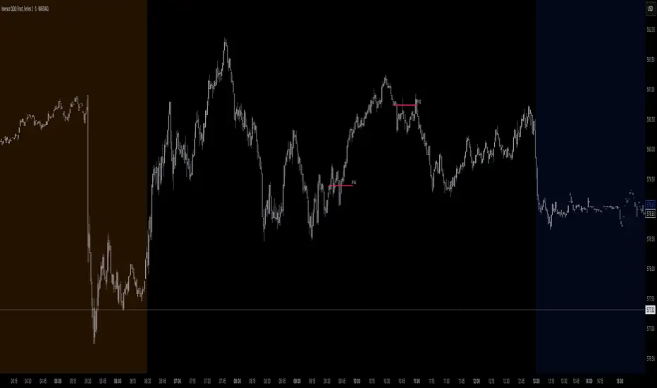
Trading Macro Windows by BW v2
Trading Macros by BW: Integrating ICT Concepts for Session Analysis
This indicator combines two key Inner Circle Trader (ICT) concepts—Change in State of Delivery (CISD) or Inverted Fair Value Gap (IFVG) signals with Macro Time Windows—to provide a unified tool for analyzing intraday price action, particularly during Pacific Time (PT) sessions. Rather than simply merging existing scripts, this integration creates a cohesive visual framework that highlights how macro consolidation periods interact with potential reversal or continuation signals like CISD or IFVG. By overlaying macro candle styling and borders on the chart alongside selectable signal lines, traders can better contextualize setups within ICT's macro narrative, where price often manipulates liquidity during these windows before displacing toward higher-timeframe objectives.
Core Components and How They Work Together:
Macro Time Windows (Inspired by ICT's Macro Periods):
ICT emphasizes "macro" as 30-minute windows (e.g., 06:45–07:15 PT, 07:45–08:15 PT, up to 11:45–12:15 PT) where price tends to consolidate, sweep liquidity, or form key structures like Fair Value Gaps (FVGs). These periods set the stage for the session's directional bias.
The indicator styles candles within these windows using a user-defined color for wicks, borders, and bodies (translucent for visibility). This visual emphasis helps traders focus on activity inside macros, where reversals or continuations often originate.
Borders are drawn as vertical lines at the start and end of each window (with a +5 minute buffer to capture related activity), using a dotted style by default. This creates a "study zone" that encapsulates macro events, allowing traders to assess if price is respecting or violating these zones in alignment with broader ICT models like the Power of 3 (AMD cycle).
Toggle: "Macro Candles Enabled" (default: true) – Turn off to disable styling and borders if focusing solely on signals.
CISD or IFVG Signals (Selectable Mode):
Mode Selection: Choose between "Change in the State of Delivery" (CISD) or "IFVG" (default: IFVG). Both detect shifts in market delivery during specific 30-minute slices (15–45 or 17–45 minutes past the hour in PT sessions).
CISD Mode: Based on ICT's definition of a sudden directional shift, this identifies aggressive displacements after sweeping recent highs/lows. It uses a rolling reference high/low over 6 bars, checks for sweeps (penetrating by at least 2 ticks in the last 2-3 bars), reclamation (closing beyond the reference with at least 50% body), and displacement (50% of prior range or an immediate FVG of 6+ ticks). Signals plot a horizontal line from the close, extending 24 bars right, labeled "CISD."
IFVG Mode: Focuses on Inverted Fair Value Gaps, where a bullish FVG (low > high by 13+ ticks) forms but is inverted (closed below) in the same slice, signaling bearish intent (or vice versa). This targets violations against opposing liquidity, often leading to raids on external ranges. Signals plot similarly, labeled "IFVG."
Shared Logic: Both modes enforce a 55-bar cooldown to prevent clustering, operate only during PT sessions (06:30–13:00), and use tick-based thresholds for precision across instruments. The integration with macros allows traders to see if signals occur within or at the edges of macro windows, enhancing confirmation—for example, a CISD inside a macro might indicate a manipulated reversal toward the session's true objective.
Toggle: "Signals Enabled" (default: true) – Turn off to hide all signal lines and labels, isolating the macro visualization.
How Components Interact:
Macro windows provide the "narrative context" (consolidation/manipulation), while CISD/IFVG signals detect the "delivery shift" (displacement). Together, they form a mashup that justifies publication: isolated signals can be noisy, but when filtered by macro periods, they align with ICT's session model. For instance, an IFVG inversion during a macro might confirm a liquidity sweep before targeting PD arrays or order blocks.
No external dependencies; all calculations are self-contained using Pine's built-in functions like ta.highest/lowest for references and time-based sessions for windows.
Usage Guidelines:
Apply to intraday charts (e.g., 1-5 min) or stocks during PT hours.
Look for confluence: A bull IFVG signal post-macro low sweep might target the next macro high or daily bias.
Customize colors/styles for signals (solid/dashed/dotted lines) and macros to suit your chart.
Backtest in replay mode to observe how macros frame signals—e.g., price often respects macro borders as S/R.
Limitations: Timezone-fixed to PT (America/Los_Angeles); signals are directional hints, not trade entries. Combine with ICT tools like order blocks or liquidity pools for full setups.
This script draws from community ICT implementations but refines them into a single, purpose-built tool for macro-driven trading, reducing chart clutter while emphasizing interconnected concepts. Feedback welcome!
The Barking Rat LiteMomentum & FVG Reversion Strategy
The Barking Rat Lite is a disciplined, short-term mean-reversion strategy that combines RSI momentum filtering, EMA bands, and Fair Value Gap (FVG) detection to identify short-term reversal points. Designed for practical use on volatile markets, it focuses on precise entries and ATR-based take profit management to balance opportunity and risk.
Core Concept
This strategy seeks potential reversals when short-term price action shows exhaustion outside an EMA band, confirmed by momentum and FVG signals:
EMA Bands:
Parameters used: A 20-period EMA (fast) and 100-period EMA (slow).
Why chosen:
- The 20 EMA is sensitive to short-term moves and reflects immediate momentum.
- The 100 EMA provides a slower, structural anchor.
When price trades outside both bands, it often signals overextension relative to both short-term and medium-term trends.
Application in strategy:
- Long entries are only considered when price dips below both EMAs, identifying potential undervaluation.
- Short entries are only considered when price rises above both EMAs, identifying potential overvaluation.
This dual-band filter avoids counter-trend signals that would occur if only a single EMA was used, making entries more selective..
Fair Value Gap Detection (FVG):
Parameters used: The script checks for dislocations using a 12-bar lookback (i.e. comparing current highs/lows with values 12 candles back).
Why chosen:
- A 12-bar displacement highlights significant inefficiencies in price structure while filtering out micro-gaps that appear every few bars in high-volatility markets.
- By aligning FVG signals with candle direction (bullish = close > open, bearish = close < open), the strategy avoids random gaps and instead targets ones that suggest exhaustion.
Application in strategy:
- Bullish FVGs form when earlier lows sit above current highs, hinting at downward over-extension.
- Bearish FVGs form when earlier highs sit below current lows, hinting at upward over-extension.
This gives the strategy a structural filter beyond simple oscillators, ensuring signals have price-dislocation context.
RSI Momentum Filter:
Parameters used: 14-period RSI with thresholds of 80 (overbought) and 20 (oversold).
Why chosen:
- RSI(14) is a widely recognized momentum measure that balances responsiveness with stability.
- The thresholds are intentionally extreme (80/20 vs. the more common 70/30), so the strategy only engages at genuine exhaustion points rather than frequent minor corrections.
Application in strategy:
- Longs trigger when RSI < 20, suggesting oversold exhaustion.
- Shorts trigger when RSI > 80, suggesting overbought exhaustion.
This ensures entries are not just technically valid but also backed by momentum extremes, raising conviction.
ATR-Based Take Profit:
Parameters used: 14-period ATR, with a default multiplier of 4.
Why chosen:
- ATR(14) reflects the prevailing volatility environment without reacting too much to outliers.
- A multiplier of 4 is a pragmatic compromise: wide enough to let trades breathe in volatile conditions, but tight enough to enforce disciplined exits before mean reversion fades.
Application in strategy:
- At entry, a fixed target is set = Entry Price ± (ATR × 4).
- This target scales automatically with volatility: narrower in calm periods, wider in explosive markets.
By avoiding discretionary exits, the system maintains rule-based discipline.
Visual Signals on Chart
Blue “▲” below candle: Potential long entry
Orange/Yellow “▼” above candle: Potential short entry
Green “✔️”: Trade closed at ATR take profit
Blue (20 EMA) & Orange (100 EMA) lines: Dynamic channel reference
⚙️Strategy report properties
Position size: 25% equity per trade
Initial capital: 10,000.00 USDT
Pyramiding: 10 entries per direction
Slippage: 2 ticks
Commission: 0.055% per side
Backtest timeframe: 1-minute
Backtest instrument: HYPEUSDT
Backtesting range: Jul 28, 2025 — Aug 17, 2025
Note on Sample Size:
You’ll notice the report displays fewer than the ideal 100 trades in the strategy report above. This is intentional. The goal of the script is to isolate high-quality, short-term reversal opportunities while filtering out low-conviction setups. This means that the Barking Rat Lite strategy is very selective, filtering out over 90% of market noise. The brief timeframe shown in the strategy report here illustrates its filtering logic over a short window — not its full capabilities. As a result, even on lower timeframes like the 1-minute chart, signals are deliberately sparse — each one must pass all criteria before triggering.
For a larger dataset:
Once the strategy is applied to your chart, users are encouraged to expand the lookback range or apply the strategy to other volatile pairs to view a full sample.
💡Why 25% Equity Per Trade?
While it's always best to size positions based on personal risk tolerance, we defaulted to 25% equity per trade in the backtesting data — and here’s why:
Backtests using this sizing show manageable drawdowns even under volatile periods.
The strategy generates a sizeable number of trades, reducing reliance on a single outcome.
Combined with conservative filters, the 25% setting offers a balance between aggression and control.
Users are strongly encouraged to customize this to suit their risk profile.
What makes Barking Rat Lite valuable
Combines multiple layers of confirmation: EMA bands + FVG + RSI
Adaptive to volatility: ATR-based exits scale with market conditions
Clear, actionable visuals: Easy to monitor and manage trades

Dual Volume Profiles: Session + Rolling (Range Delineation)Dual Volume Profiles: Session + Rolling (Range Delineation)
INTRO
This is a probability-centric take on volume profile. I treat the volume histogram as an empirical PDF over price, updated in real time, which makes multi-modality (multiple acceptance basins) explicit rather than assumed away. The immediate benefit is operational: if we can read the shape of the distribution, we can infer likely reversion levels (POC), acceptance boundaries (VAH/VAL), and low-friction corridors (LVNs).
My working hypothesis is that what traders often label “fat tails” or “power-law behavior” at short horizons is frequently a tail-conditioned view of a higher-level Gaussian regime. In other words, child distributions (shorter periodicities) sit within parent distributions (longer periodicities); when price operates in the parent’s tail, the child regime looks heavy-tailed without being fundamentally non-Gaussian. This is consistent with a hierarchical/mixture view and with the spirit of the central limit theorem—Gaussian structure emerges at aggregate scales, while local scales can look non-Gaussian due to nesting and conditioning.
This indicator operationalizes that view by plotting two nested empirical PDFs: a rolling (local) profile and a session-anchored profile. Their confluence makes ranges explicit and turns “regime” into something you can see. For additional nesting, run multiple instances with different lookbacks. When using the default settings combined with a separate daily VP, you effectively get three nested distributions (local → session → daily) on the chart.
This indicator plots two nested distributions side-by-side:
Rolling (Local) Profile — short-window, prorated histogram that “breathes” with price and maps the immediate auction.
Session Anchored Profile — cumulative distribution since the current session start (Premkt → RTH → AH anchoring), revealing the parent regime.
Use their confluence to identify range floors/ceilings, mean-reversion magnets, and low-volume “air pockets” for fast traverses.
What it shows
POC (dashed): central tendency / “magnet” (highest-volume bin).
VAH & VAL (solid): acceptance boundaries enclosing an exact Value Area % around each profile’s POC.
Volume histograms:
Rolling can auto-color by buy/sell dominance over the lookback (green = buying ≥ selling, red = selling > buying).
Session uses a fixed style (blue by default).
Session anchoring (exchange timezone):
Premarket → anchors at 00:00 (midnight).
RTH → anchors at 09:30.
After-hours → anchors at 16:00.
Session display span:
Session Max Span (bars) = 0 → draw from session start → now (anchored).
> 0 → draw a rolling window N bars back → now, while still measuring all volume since session start.
Why it’s useful
Think in terms of nested probability distributions: the rolling node is your local Gaussian; the session node is its parent.
VA↔VA overlap ≈ strong range boundary.
POC↔POC alignment ≈ reliable mean-reversion target.
LVNs (gaps) ≈ low-friction corridors—expect quick moves to the next node.
Quick start
Add to chart (great on 5–10s, 15–60s, 1–5m).
Start with: bins = 240, vaPct = 0.68, barsBack = 60.
Watch for:
First test & rejection at overlapping VALs/VAHs → fade back toward POC.
Acceptance beyond VA (several closes + growing outer-bin mass) → traverse to the next node.
Inputs (detailed)
General
Lookback Bars (Rolling)
Count of most-recent bars for the rolling/local histogram. Larger = smoother node that shifts slower; smaller = more reactive, “breathing” profile.
• Typical: 40–80 on 5–10s charts; 60–120 on 1–5m.
• If you increase this but keep Number of Bins fixed, each bin aggregates more volume (coarser bins).
Number of Bins
Vertical resolution (price buckets) for both rolling and session histograms. Higher = finer detail and crisper LVNs, but more line objects (closer to platform limits).
• Typical: 120–240 on 5–10s; 80–160 on 1–5m.
• If you hit performance or object limits, reduce this first.
Value Area %
Exact central coverage for VAH/VAL around POC. Computed empirically from the histogram (no Gaussian assumption): the algorithm expands from POC outward until the chosen % is enclosed.
• Common: 0.68 (≈“1σ-like”), 0.70 for slightly wider core.
• Smaller = tighter VA (more breakout flags). Larger = wider VA (more reversion bias).
Max Local Profile Width (px)
Horizontal length (in pixels) of the rolling bars/lines and its VA/POC overlays. Visual only (does not affect calculations).
Session Settings
RTH Start/End (exchange tz)
Defines the current session anchor (Premkt=00:00, RTH=your start, AH=your end). The session histogram always measures from the most recent session start and resets at each boundary.
Session Max Span (bars, 0 = full session)
Display window for session drawings (POC/VA/Histogram).
• 0 → draw from session start → now (anchored).
• > 0 → draw N bars back → now (rolling look), while still measuring all volume since session start.
This keeps the “parent” distribution measurable while letting the display track current action.
Local (Rolling) — Visibility
Show Local Profile Bars / POC / VAH & VAL
Toggle each overlay independently. If you approach object limits, disable bars first (POC/VA lines are lighter).
Local (Rolling) — Colors & Widths
Color by Buy/Sell Dominance
Fast uptick/downtick proxy over the rolling window (close vs open):
• Buying ≥ Selling → Bullish Color (default lime).
• Selling > Buying → Bearish Color (default red).
This color drives local bars, local POC, and local VA lines.
• Disable to use fixed Bars Color / POC Color / VA Lines Color.
Bars Transparency (0–100) — alpha for the local histogram (higher = lighter).
Bars Line Width (thickness) — draw thin-line profiles or chunky blocks.
POC Line Width / VA Lines Width — overlay thickness. POC is dashed, VAH/VAL solid by design.
Session — Visibility
Show Session Profile Bars / POC / VAH & VAL
Independent toggles for the session layer.
Session — Colors & Widths
Bars/POC/VA Colors & Line Widths
Fixed palette by design (default blue). These do not change with buy/sell dominance.
• Use transparency and width to make the parent profile prominent or subtle.
• Prefer minimal? Hide session bars; keep only session VA/POC.
Reading the signals (detailed playbook)
Core definitions
POC — highest-volume bin (fair price “magnet”).
VAH/VAL — upper/lower bounds enclosing your Value Area % around POC.
Node — contiguous block of high-volume bins (acceptance).
LVN — low-volume gap between nodes (low friction path).
Rejection vs Acceptance (practical rule)
Rejection at VA edge: 0–1 closes beyond VA and no persistent growth in outer bins.
Acceptance beyond VA: ≥3 closes beyond VA and outer-bin mass grows (e.g., added volume beyond the VA edge ≥ 5–10% of node volume over the last N bars). Treat acceptance as regime change.
Confluence scores (make boundary/target quality objective)
VA overlap strength (range boundary):
C_VA = 1 − |VA_edge_local − VA_edge_session| / ATR(n)
Values near 1.0 = tight overlap (stronger boundary).
Use: if C_VA ≥ 0.6–0.8, treat as high-quality fade zone.
POC alignment (magnet quality):
C_POC = 1 − |POC_local − POC_session| / ATR(n)
Higher C_POC = greater chance a rotation completes to that fair price.
(You can estimate these by eye.)
Setups
1) Range Fade at VA Confluence (mean reversion)
Context: Local VAL/VAH near Session VAL/VAH (tight overlap), clear node, local color not screaming trend (or flips to your side).
Entry: First test & rejection at the overlapped band (wick through ok; prefer close back inside).
Stop: A tick/pip beyond the wider of the two VA edges or beyond the nearest LVN, a small buffer zone can be used to judge whether price is truly rejecting a VAL/VAH or simply probing.
Targets: T1 node mid; T2 POC (size up when C_POC is high).
Flip: If acceptance (rule above) prints, flip bias or stand down.
2) LVN Traverse (continuation)
Context: Price exits VA and enters an LVN with acceptance and growing outer-bin volume.
Entry: Aggressive—first close into LVN; Conservative—retest of the VA edge from the far side (“kiss goodbye”).
Stop: Back inside the prior VA.
Targets: Next node’s VA edge or POC (edge = faster exits; POC = fuller rotations).
Note: Flatter VA edge (shallower curvature) tends to breach more easily.
3) POC→POC Magnet Trade (rotation completion)
Context: Local POC ≈ Session POC (high C_POC).
Entry: Fade a VA touch or pullback inside node, aiming toward the shared POC.
Stop: Past the opposite VA edge or LVN beyond.
Target: The shared POC; optional runner to opposite VA if the node is broad and time-of-day is supportive.
4) Failed Break (Reversion Snap-back)
Context: Push beyond VA fails acceptance (re-enters VA, outer-bin growth stalls/shrinks).
Entry: On the re-entry close, back toward POC.
Stop/Target: Stop just beyond the failed VA; target POC, then opposite VA if momentum persists.
How to read color & shape
Local color = most recent sentiment:
Green = buying ≥ selling; Red = selling > buying (over the rolling window). Treat as context, not a standalone signal. A green local node under a blue session VAH can still be a fade if the parent says “over-valued.”
Shape tells friction:
Fat nodes → rotation-friendly (fade edges).
Sharp LVN gaps → traversal-friendly (momentum continuation).
Time-of-day intuition
Right after session anchor (e.g., RTH 09:30): Session profile is young and moves quickly—treat confluence cautiously.
Mid-session: Cleanest behavior for rotations.
Close / news: Expect more traverses and POC migrations; tighten risk or switch playbooks.
Risk & execution guidance
Use tight, mechanical stops at/just beyond VA or LVN. If you need wide stops to survive noise, your entry is late or the node is unstable.
On micro-timeframes, account for fees & slippage—aim for targets paying ≥2–3× average cost.
If acceptance prints, don’t fight it—flip, reduce size, or stand aside.
Suggested presets
Scalp (5–10s): bins 120–240, barsBack 40–80, vaPct 0.68–0.70, local bars thin (small bar width).
Intraday (1–5m): bins 80–160, barsBack 60–120, vaPct 0.68–0.75, session bars more visible for parent context.
Performance & limits
Reuses line objects to stay under TradingView’s max_lines_count.
Very large bins × multiple overlays can still hit limits—use visibility toggles (hide bars first).
Session drawings use time-based coordinates to avoid “bar index too far” errors.
Known nuances
Rolling buy/sell dominance uses a simple uptick/downtick proxy (close vs open). It’s fast and practical, but it’s not a full tape classifier.
VA boundaries are computed from the empirical histogram—no Gaussian assumption.
This script does not calculate the full daily volume profile. Several other tools already provide that, including TradingView’s built-in Volume Profile indicators. Instead, this indicator focuses on pairing a rolling, short-term volume distribution with a session-wide distribution to make ranges more explicit. It is designed to supplement your use of standard or periodic volume profiles, not replace them. Think of it as a magnifying lens that helps you see where local structure aligns with the broader session.
How to trade it (TL;DR)
Fade overlapping VA bands on first rejection → target POC.
Continue through LVN on acceptance beyond VA → target next node’s VA/POC.
Respect acceptance: ≥3 closes beyond VA + growing outer-bin volume = regime change.
FAQ
Q: Why 68% Value Area?
A: It mirrors the “~1σ” idea, but we compute it exactly from empirical volume, not by assuming a normal distribution.
Q: Why are my profiles thin lines?
A: Increase Bars Line Width for chunkier blocks; reduce for fine, thin-line profiles.
Q: Session bars don’t reach session start—why?
A: Set Session Max Span (bars) = 0 for full anchoring; any positive value draws a rolling window while still measuring from session start.
Changelog (v1.0)
Dual profiles: Rolling + Session with independent POC/VA lines.
Session anchoring (Premkt/RTH/AH) with optional rolling display span.
Dynamic coloring for the rolling profile (buying vs selling).
Fully modular toggles + per-feature colors/widths.
Thin-line rendering via bar line width.

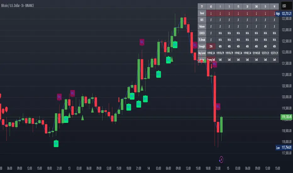
XAUUSD Strength Dashboard with VolumeXAUUSD Strength Dashboard with Volume Analysis
📌 Description
This advanced Pine Script indicator provides a multi-timeframe dashboard for XAUUSD (Gold vs. USD), combining price action analysis with volume confirmation to generate high-probability trading signals. It detects:
✅ Break of Structure (BOS)
✅ Fair Value Gaps (FVG)
✅ Change of Character (CHOCH)
✅ Trendline Breaks (9/21 SMA Crossover)
✅ Volume Spikes (Confirmation of Strength)
The dashboard displays strength scores (0-100%) and action recommendations (Strong Buy/Buy/Neutral/Sell/Strong Sell) across multiple timeframes, helping traders identify confluences for better trade decisions.
🎯 How It Works
1. Multi-Timeframe Analysis
Fetches data from 1m, 5m, 15m, 30m, 1h, 4h, Daily, and Weekly timeframes.
Compares trend direction, BOS, FVG, CHOCH, and volume spikes across all timeframes.
2. Volume-Confirmed Strength Score
The Strength Score (0-100%) is calculated using:
Trend Direction (25 points) → 9 SMA vs. 21 SMA
Break of Structure (20 points) → New highs/lows with momentum
Fair Value Gaps (10 points) → Imbalance zones
Change of Character (10 points) → Shift in market structure
Trendline Break (20 points) → SMA crossover confirmation
Volume Spike (15 points) → High volume confirms moves
Score Interpretation:
≥75% → Strong Buy (High confidence bullish move)
60-74% → Buy (Bullish but weaker confirmation)
40-59% → Neutral (No strong bias)
25-39% → Sell (Bearish but weaker confirmation)
≤25% → Strong Sell (High confidence bearish move)
3. Dashboard & Chart Markers
Dashboard Table: Shows Trend, BOS, Volume, CHOCH, TL Break, Strength %, Key Level, and Action for each timeframe.
Chart Markers:
🟢 Green Triangles → Bullish BOS
🔴 Red Triangles → Bearish BOS
🟢 Green Circles → Bullish CHOCH
🔴 Red Circles → Bearish CHOCH
📈 Green Arrows → Bullish Trendline Break
📉 Red Arrows → Bearish Trendline Break
"Vol↑" (Lime) → Bullish Volume Spike
"Vol↓" (Maroon) → Bearish Volume Spike
🚀 How to Use
1. Dashboard Interpretation
Higher Timeframes (D/W) → Show the dominant trend.
Lower Timeframes (1m-4h) → Help with entry timing.
Strength Score ≥75% or ≤25% → Look for high-confidence trades.
Volume Spikes → Confirm breakouts/reversals.
2. Trading Strategy
📈 Long (Buy) Setup:
Higher TFs (D/W/4h) show bullish trend (↑).
Current TF has BOS & Volume Spike.
Strength Score ≥60%.
Key Level (Low) holds as support.
📉 Short (Sell) Setup:
Higher TFs (D/W/4h) show bearish trend (↓).
Current TF has BOS & Volume Spike.
Strength Score ≤40%.
Key Level (High) holds as resistance.
3. Customization
Adjust Volume Spike Multiplier (Default: 1.5x) → Controls sensitivity to volume spikes.
Toggle Timeframes → Enable/disable higher/lower timeframes.
🔑 Key Benefits
✔ Multi-Timeframe Confluence → Avoids false signals.
✔ Volume Confirmation → Filters low-quality breakouts.
✔ Clear Strength Scoring → Removes emotional bias.
✔ Visual Chart Markers → Easy to spot key signals.
This indicator is ideal for gold traders who follow institutional order flow, market structure, and volume analysis to improve their trading decisions.
🎯 Best Used With:
Support/Resistance Levels
Fibonacci Retracements
Price Action Confirmation
🚀 Happy Trading! 🚀
ICT SMC Custom — BOS/MSS + OB + FVGWant me to fill that box? Here’s a ready‑to‑paste description for your publish screen:
⸻
ICT SMC Custom — BOS/MSS + OB + FVG (Crypto‑friendly)
A clean Smart Money Concepts tool that marks Break of Structure (BOS), Market Structure Shift (MSS), Order Blocks (OB), and Fair Value Gaps (FVG) with bold, easy‑to‑see visuals. Built for crypto but works on any market and timeframe.
What it does
• BOS & MSS detection with optional body/wick logic
• Order Blocks: auto‑draws the last opposite candle before a BOS, keeps only the most recent N, and fades when mitigated
• FVGs: 3‑candle gaps with a minimum size filter and a cap on how many to keep
• HTF Swings (optional): plots higher‑timeframe pivot highs/lows for top‑down context
• Alerts for BOS/MSS and FVG formation
Inputs
• Swing pivot length (default 3): sensitivity for structure pivots
• Use candle bodies for breaks: close vs level (on) or wicks (off)
• Show BOS/MSS labels, Show FVG, Show Order Blocks
• Min FVG size (ticks) and Max boxes to keep for FVG/OB
• OB uses candle body: body range vs full wick range
• Show higher timeframe swings + HTF timeframe
• Bullish/Bearish colors
How it works
• BOS triggers when price breaks the last opposite swing.
• MSS flags when the break flips the prior bias.
• OB is the most recent opposite candle prior to BOS; it’s marked and later greyed out once price closes through it (mitigation).
• FVG is detected when candle 1’s high < candle 3’s low (bear) or candle 1’s low > candle 3’s high (bull).
Alerts included
• BOS Up / BOS Down
• MSS Up / MSS Down
• FVG Up / FVG Down
Tips
• Start on 15m/1h for crypto, pivot length 3–5.
• Turn Use candle bodies ON for stricter confirmations, OFF for more signals.
• If boxes look cluttered, lower “Max boxes to keep.”
Note: This is a visual/educational tool, not financial advice. Always confirm with your own plan and risk management.

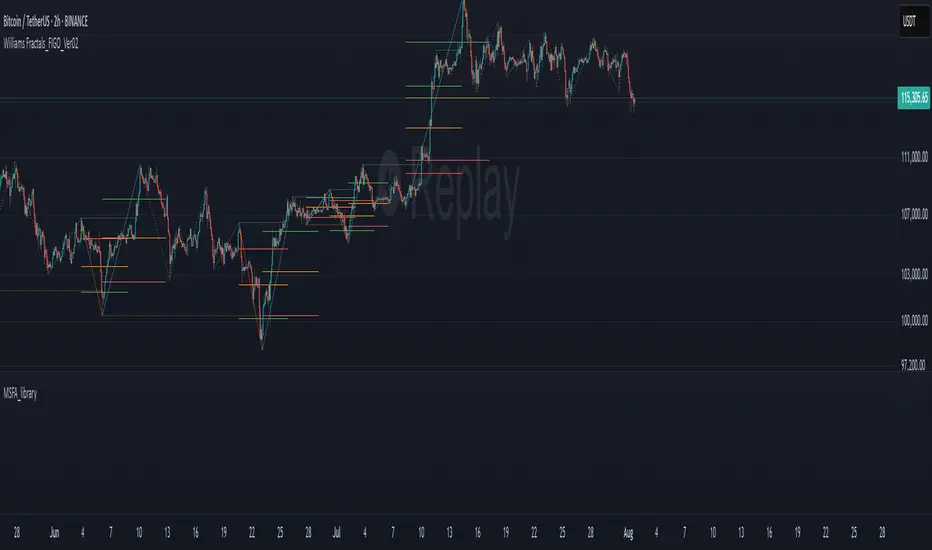
MSFA_LibraryLibrary "MSFA_library"
TODO: add library description here
getDecimals()
Calculates how many decimals are on the quote price of the current market
Returns: The current decimal places on the market quote price
getPipSize(multiplier)
Calculates the pip size of the current market
Parameters:
multiplier (int) : The mintick point multiplier (1 by default, 10 for FX/Crypto/CFD but can be used to override when certain markets require)
Returns: The pip size for the current market
truncate(number, decimalPlaces)
Truncates (cuts) excess decimal places
Parameters:
number (float) : The number to truncate
decimalPlaces (simple float) : (default=2) The number of decimal places to truncate to
Returns: The given number truncated to the given decimalPlaces
toWhole(number)
Converts pips into whole numbers
Parameters:
number (float) : The pip number to convert into a whole number
Returns: The converted number
toPips(number)
Converts whole numbers back into pips
Parameters:
number (float) : The whole number to convert into pips
Returns: The converted number
getPctChange(value1, value2, lookback)
Gets the percentage change between 2 float values over a given lookback period
Parameters:
value1 (float) : The first value to reference
value2 (float) : The second value to reference
lookback (int) : The lookback period to analyze
Returns: The percent change over the two values and lookback period
random(minRange, maxRange)
Wichmann–Hill Pseudo-Random Number Generator
Parameters:
minRange (float) : The smallest possible number (default: 0)
maxRange (float) : The largest possible number (default: 1)
Returns: A random number between minRange and maxRange
bullFib(priceLow, priceHigh, fibRatio)
Calculates a bullish fibonacci value
Parameters:
priceLow (float) : The lowest price point
priceHigh (float) : The highest price point
fibRatio (float) : The fibonacci % ratio to calculate
Returns: The fibonacci value of the given ratio between the two price points
bearFib(priceLow, priceHigh, fibRatio)
Calculates a bearish fibonacci value
Parameters:
priceLow (float) : The lowest price point
priceHigh (float) : The highest price point
fibRatio (float) : The fibonacci % ratio to calculate
Returns: The fibonacci value of the given ratio between the two price points
getMA(length, maType)
Gets a Moving Average based on type (! MUST BE CALLED ON EVERY TICK TO BE ACCURATE, don't place in scopes)
Parameters:
length (simple int) : The MA period
maType (string) : The type of MA
Returns: A moving average with the given parameters
barsAboveMA(lookback, ma)
Counts how many candles are above the MA
Parameters:
lookback (int) : The lookback period to look back over
ma (float) : The moving average to check
Returns: The bar count of how many recent bars are above the MA
barsBelowMA(lookback, ma)
Counts how many candles are below the MA
Parameters:
lookback (int) : The lookback period to look back over
ma (float) : The moving average to reference
Returns: The bar count of how many recent bars are below the EMA
barsCrossedMA(lookback, ma)
Counts how many times the EMA was crossed recently (based on closing prices)
Parameters:
lookback (int) : The lookback period to look back over
ma (float) : The moving average to reference
Returns: The bar count of how many times price recently crossed the EMA (based on closing prices)
getPullbackBarCount(lookback, direction)
Counts how many green & red bars have printed recently (ie. pullback count)
Parameters:
lookback (int) : The lookback period to look back over
direction (int) : The color of the bar to count (1 = Green, -1 = Red)
Returns: The bar count of how many candles have retraced over the given lookback & direction
getBodySize()
Gets the current candle's body size (in POINTS, divide by 10 to get pips)
Returns: The current candle's body size in POINTS
getTopWickSize()
Gets the current candle's top wick size (in POINTS, divide by 10 to get pips)
Returns: The current candle's top wick size in POINTS
getBottomWickSize()
Gets the current candle's bottom wick size (in POINTS, divide by 10 to get pips)
Returns: The current candle's bottom wick size in POINTS
getBodyPercent()
Gets the current candle's body size as a percentage of its entire size including its wicks
Returns: The current candle's body size percentage
isHammer(fib, colorMatch)
Checks if the current bar is a hammer candle based on the given parameters
Parameters:
fib (float) : (default=0.382) The fib to base candle body on
colorMatch (bool) : (default=false) Does the candle need to be green? (true/false)
Returns: A boolean - true if the current bar matches the requirements of a hammer candle
isStar(fib, colorMatch)
Checks if the current bar is a shooting star candle based on the given parameters
Parameters:
fib (float) : (default=0.382) The fib to base candle body on
colorMatch (bool) : (default=false) Does the candle need to be red? (true/false)
Returns: A boolean - true if the current bar matches the requirements of a shooting star candle
isDoji(wickSize, bodySize)
Checks if the current bar is a doji candle based on the given parameters
Parameters:
wickSize (float) : (default=2) The maximum top wick size compared to the bottom (and vice versa)
bodySize (float) : (default=0.05) The maximum body size as a percentage compared to the entire candle size
Returns: A boolean - true if the current bar matches the requirements of a doji candle
isBullishEC(allowance, rejectionWickSize, engulfWick)
Checks if the current bar is a bullish engulfing candle
Parameters:
allowance (float) : (default=0) How many POINTS to allow the open to be off by (useful for markets with micro gaps)
rejectionWickSize (float) : (default=disabled) The maximum rejection wick size compared to the body as a percentage
engulfWick (bool) : (default=false) Does the engulfing candle require the wick to be engulfed as well?
Returns: A boolean - true if the current bar matches the requirements of a bullish engulfing candle
isBearishEC(allowance, rejectionWickSize, engulfWick)
Checks if the current bar is a bearish engulfing candle
Parameters:
allowance (float) : (default=0) How many POINTS to allow the open to be off by (useful for markets with micro gaps)
rejectionWickSize (float) : (default=disabled) The maximum rejection wick size compared to the body as a percentage
engulfWick (bool) : (default=false) Does the engulfing candle require the wick to be engulfed as well?
Returns: A boolean - true if the current bar matches the requirements of a bearish engulfing candle
isInsideBar()
Detects inside bars
Returns: Returns true if the current bar is an inside bar
isOutsideBar()
Detects outside bars
Returns: Returns true if the current bar is an outside bar
barInSession(sess, useFilter)
Determines if the current price bar falls inside the specified session
Parameters:
sess (simple string) : The session to check
useFilter (bool) : (default=true) Whether or not to actually use this filter
Returns: A boolean - true if the current bar falls within the given time session
barOutSession(sess, useFilter)
Determines if the current price bar falls outside the specified session
Parameters:
sess (simple string) : The session to check
useFilter (bool) : (default=true) Whether or not to actually use this filter
Returns: A boolean - true if the current bar falls outside the given time session
dateFilter(startTime, endTime)
Determines if this bar's time falls within date filter range
Parameters:
startTime (int) : The UNIX date timestamp to begin searching from
endTime (int) : the UNIX date timestamp to stop searching from
Returns: A boolean - true if the current bar falls within the given dates
dayFilter(monday, tuesday, wednesday, thursday, friday, saturday, sunday)
Checks if the current bar's day is in the list of given days to analyze
Parameters:
monday (bool) : Should the script analyze this day? (true/false)
tuesday (bool) : Should the script analyze this day? (true/false)
wednesday (bool) : Should the script analyze this day? (true/false)
thursday (bool) : Should the script analyze this day? (true/false)
friday (bool) : Should the script analyze this day? (true/false)
saturday (bool) : Should the script analyze this day? (true/false)
sunday (bool) : Should the script analyze this day? (true/false)
Returns: A boolean - true if the current bar's day is one of the given days
atrFilter(atrValue, maxSize)
Parameters:
atrValue (float)
maxSize (float)
tradeCount()
Calculate total trade count
Returns: Total closed trade count
isLong()
Check if we're currently in a long trade
Returns: True if our position size is positive
isShort()
Check if we're currently in a short trade
Returns: True if our position size is negative
isFlat()
Check if we're currentlyflat
Returns: True if our position size is zero
wonTrade()
Check if this bar falls after a winning trade
Returns: True if we just won a trade
lostTrade()
Check if this bar falls after a losing trade
Returns: True if we just lost a trade
maxDrawdownRealized()
Gets the max drawdown based on closed trades (ie. realized P&L). The strategy tester displays max drawdown as open P&L (unrealized).
Returns: The max drawdown based on closed trades (ie. realized P&L). The strategy tester displays max drawdown as open P&L (unrealized).
totalPipReturn()
Gets the total amount of pips won/lost (as a whole number)
Returns: Total amount of pips won/lost (as a whole number)
longWinCount()
Count how many winning long trades we've had
Returns: Long win count
shortWinCount()
Count how many winning short trades we've had
Returns: Short win count
longLossCount()
Count how many losing long trades we've had
Returns: Long loss count
shortLossCount()
Count how many losing short trades we've had
Returns: Short loss count
breakEvenCount(allowanceTicks)
Count how many break-even trades we've had
Parameters:
allowanceTicks (float) : Optional - how many ticks to allow between entry & exit price (default 0)
Returns: Break-even count
longCount()
Count how many long trades we've taken
Returns: Long trade count
shortCount()
Count how many short trades we've taken
Returns: Short trade count
longWinPercent()
Calculate win rate of long trades
Returns: Long win rate (0-100)
shortWinPercent()
Calculate win rate of short trades
Returns: Short win rate (0-100)
breakEvenPercent(allowanceTicks)
Calculate break even rate of all trades
Parameters:
allowanceTicks (float) : Optional - how many ticks to allow between entry & exit price (default 0)
Returns: Break-even win rate (0-100)
averageRR()
Calculate average risk:reward
Returns: Average winning trade divided by average losing trade
unitsToLots(units)
(Forex) Convert the given unit count to lots (multiples of 100,000)
Parameters:
units (float) : The units to convert into lots
Returns: Units converted to nearest lot size (as float)
skipTradeMonteCarlo(chance, debug)
Checks to see if trade should be skipped to emulate rudimentary Monte Carlo simulation
Parameters:
chance (float) : The chance to skip a trade (0-1 or 0-100, function will normalize to 0-1)
debug (bool) : Whether or not to display a label informing of the trade skip
Returns: True if the trade is skipped, false if it's not skipped (idea being to include this function in entry condition validation checks)
fillCell(tableID, column, row, title, value, bgcolor, txtcolor, tooltip)
This updates the given table's cell with the given values
Parameters:
tableID (table) : The table ID to update
column (int) : The column to update
row (int) : The row to update
title (string) : The title of this cell
value (string) : The value of this cell
bgcolor (color) : The background color of this cell
txtcolor (color) : The text color of this cell
tooltip (string)
Returns: Nothing.
Fair Value MSThis indicator introduces rigid rules to familiar concepts to better capture and visualize Market Structure and Areas of Support and Resistance in a way that is both rule-based and reactive to market movements.
Typical "Market Structure" or "Zig-Zag" methods determine swing points based on fixed thresholds (length or percentage). While this does provide rigid structure, the results may be lagging or confusing due to the timing, since it is fixed to static parameters.
I believe the concept of Fair Value Gaps can solve this problem.
As you will notice, there are no length settings in this indicator.
> FVG Market Structure
Fair Value Gaps are a well known concept used to indicate directional intent, forming when price moves aggressively in one direction, leaving behind an imbalance between buyers and sellers. While the term FVG was popularized by ICT, the underlying concept predates them, known historically as imbalances, inefficiencies, or liquidity voids in institutional trading.
Note: For simplicity, in this indicator they'll be called FVGs.
By reading into this, we are able to clearly and rigidly define market structure simply by "looking" at the chart, using objective price events rather than subjective interpretation, or lengths.
By using FVGs to determine structure direction, the length, and speed of identification lies entirely on the market. If an FVG Down occurs immediately after a New Higher High forms, it is reasonable to assume there was a seller at that point, so the script would indicate a New Swing High.
The script is NOT stuck, waiting for a % retrace, or # bars to pass to identify it as such.
Sometimes the market is in a steady trend in a single direction and no FVGs form; therefore, no structure forms. -> Why would we try to impose structure on a clear trend?
Ultimately, the FVG Structure Method uses real reactions from the market to determine Market structure, and is not fixed to specific parameters.
As with other market structure indicators, "Market Structure Breaks" are still identifiable when price moves outside the most recent swing points.
These are helpful to indicate larger direction. In the following section you will see how these help us determine when we should start the search for an "Area of Interest (AOI)".
> Areas of Interest (AOIs)
"Area of Interest (AOI)" is a generalized term, and could refer to many types of zones you might recognize under different names. While the AOIs in this indicator are specialized in their own way, I have chosen to simply use the term "Area of Interest" because it’s more important to understand how they behave and why they exist than to focus on what they’re called.
The goal of an AOI is to point out reasonable areas where buyers or sellers may be staging, as is typical with support and resistance.
In order to reasonably identify these areas, we look for cause and effect relationships. When considering these relationships, it's easier to understand the placement of the points to define each zone.
(Buyer Examples)
Cause: Strong Buyers step in at Swing Low
Effect: Fair Value Gap Forms
Cause: Sustained Buying Pressure
Effect: Market Structure Breaks
In this example, The zone is drawn from the Swing Low, to the Bottom of the FVG closest to the swing point.
In theory, the participation at the swing point was strong and aggressive enough to create the FVG imbalance. Which then found acceptance and continued into a Market Structure Break. So with these AOIs, we are trying to locate the aggressive Buyers or Sellers which were positioned BEFORE the FVG.
These Zones are intended to act as areas to look for reactions from market participants, to judge where price may be going. When revisiting these zones, we look for a reaction or a break, to further provide us information to if the buyers or sellers are still there.
As seen in the screenshot above, The information we gain is not from the creation of these zones, but from the behavior we witness when these zones are revisited.
Technical Note: In this indicator, Market Structure Breaks are only considered when price closes outside the recent swing points. Wicks are not considered as confirmation, therefore are not used to detect structural breaks.
Inside each AOI you can optionally display a readout of the volume which accumulated during the time starting at the swing point and going until the closing bar of the FVG.
Note: We are counting volume until the closing bar of the FVG since the FVG is a 3 bar formation, and aggressive volume is required throughout to create the imbalance.
There are multiple FVGs that typically occur in a single direction, but we do not look to every single one to be indicative of structure, only the first FVG in the opposite direction of the previous direction (which is determined by previous FVGs)
You will probably notice, the AOIs do not form from the closest swing or FVG to the break, this is because we are targeting larger directional changes to draw these AOIs from.
Since they do not always happen perfectly every time, the AOI formation waits for an FVG to occur AND a Market structure break to happen. One without the other will result in no Zone displaying.
> Reflection Lines
While they may seem slightly redundant, Reflection Lines serve as reminders of previous support and resistance pivots. They are drawn at the same Pivots where and AOI is formed, and extend beyond the mitigation of the AOI.
These lines are often points of price to look for "Support Flips", a re-test pattern where price trades through previous support (or resistance) then returns to it and rejects, continuing into a larger move or trend.
Their namesake is based on the behavior of price, "reflecting" at these levels.
The Reflection lines are simple and change color based on price's location.
If price is above, we would typically look to a reflection line in with support in mind.
As a basic filter, these lines use an average price to determine their color, this way they will not change their color as frequently in choppy situations.
> Session Start/End Lines
For analysis purposes and trade review, it is helpful to analyze with context.
For that reason, I have implemented start and end session lines into the indicator, these are helpful when reviewing historical charts to not provide additional context.
By default, they are set to the NYSE Session, but can be changed to fit any needs.
These lines are not advanced, and simply draw a line as the chart passes the start and end of the sessions. It's very likely that you may need to adjust the session for your specific needs.
Note: The Timezone can be adjusted within the code if needed. By Default, the indicator uses "America/New_York" Timezone.
> Conclusion
If you’ve ever felt like your structure tools were confusing or lagging, drawing zones too late, or zones that simply don't make sense, this should feel like a breath of fresh air.
By removing arbitrary length settings and instead using FVGs to define structure and as a basis for AOIs, you're getting a more accurate look at what price is doing and where it's reacting from.
This indicator is rule-based, reactive, and aims to keep things logical without fluff or false confidence.
Enjoy!

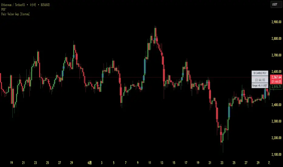
Fair Value Gap [Custom]📌 FVG Indicator – Smart Money Concepts Tool
This script is based on Smart Money Concepts (SMC) and automatically detects and marks Fair Value Gaps (FVG) on the chart, helping traders identify unbalanced price areas left behind by institutional moves.
🧠 What is an FVG?
An FVG (Fair Value Gap) is the price gap formed when the market moves rapidly, leaving behind a candle range where no trading occurred — typically between Candle 1’s high and Candle 3’s low (in a three-candle pattern). These gaps often signal imbalance, created during structural breaks or liquidity grabs, and may act as retrace zones or entry points.
🛠 Features:
✅ Automatically detects and highlights FVG zones (high-low range)
✅ Differentiates between open (unfilled) and closed (filled) FVGs
✅ Adjustable timeframe settings (works best on 1H–4H charts)
✅ Option to toggle display of filled FVGs
✅ Great for identifying pullback entries, continuation zones, or reversal setups
💡 Recommended Use:
After BOS/CHoCH, watch for price to return to the FVG for entry
Combine with Order Blocks and liquidity zones for higher accuracy
Best used as part of an ICT or SMC-based trading system
Dynamic Gap Probability ToolDynamic Gap Probability Tool measures the percentage gap between price and a chosen moving average, then analyzes your chart history to estimate the likelihood of the next candle moving up or down. It dynamically adjusts its sample size to ensure statistical robustness while focusing on the exact deviation level.
Originality and Value:
• Combines gap-based analysis with dynamic sample aggregation to balance precision and reliability.
• Automatically extends the sample when exact matches are scarce, avoiding misleading signals on rare extreme moves.
• Provides real “next-candle” probabilities based on historical occurrences rather than fixed thresholds or untested heuristics.
• Adds value by giving traders an evidence-based edge: you see how similar past deviations actually played out.
How It Works:
1. Calculate gap = (close – moving average) / moving average * 100.
2. Round the absolute gap to nearest percent (X%).
3. Count historical bars where gap ≥ X% above or ≤ –X% below.
4. If exact X% count is below the minimum occurrences threshold, include gaps at X+1%, X+2%, etc., until threshold is reached.
5. Compute “next-candle” green vs. red probabilities from the aggregated sample.
6. Display current gap, sample size, green probability, and red probability in a table.
Inputs:
• Moving Average Type (SMA, EMA, WMA, VWMA, HMA, SMMA, TMA)
• Moving Average Period (default 200)
• Minimum Occurrences Threshold (default 50)
• Table position and styling options
Examples:
• If price is 3% above the 200-period SMA and 120 occurrences ≥3% are found, with 84 green next candles (70%) and 36 red (30%), the script displays “3% | 120 | 70% green | 30% red.”
• If price is 8% below the SMA but only 20 exact matches exist, the script will include 9% and 10% gaps until it reaches 50 samples, then calculate probabilities from that broader set.
Why It’s Useful:
• Mean-reversion traders see green-probability signals at extreme overbought or oversold levels.
• Trend-followers identify continuation likelihood when red probability is high.
• Risk managers gauge reliability by inspecting sample size before acting on any signal.
Limitations:
• Historical probabilities do not guarantee future performance.
• Results depend on timeframe and symbol, backtest with your data before trading.
• Use realistic slippage and commission when overlaying on strategy scripts.

Normalized Open InterestNormalized Open Interest (nOI) — Indicator Overview
What it does
Normalized Open Interest (nOI) transforms raw futures open-interest data into a 0-to-100 oscillator, so you can see at a glance whether participation is unusually high or low—similar in spirit to an RSI but applied to open interest. The script positions today’s OI inside a rolling high–low range and paints it with contextual colours.
Core logic
Data source – Loads the built-in “_OI” symbol that TradingView provides for the current market.
Rolling range – Looks back a user-defined number of bars (default 500) to find the highest and lowest OI in that window.
Normalization – Calculates
nOI = (OI – lowest) / (highest – lowest) × 100
so 0 equals the minimum of the window and 100 equals the maximum.
Visual cues – Plots the oscillator plus fixed horizontal levels at 70 % and 30 % (or your own numbers). The line turns teal above the upper level, red below the lower, and neutral grey in between.
User inputs
Window Length (bars) – How many candles the indicator scans for the high–low range; larger numbers smooth the curve, smaller numbers make it more reactive.
Upper Threshold (%) – Default 70. Anything above this marks potentially crowded or overheated interest.
Lower Threshold (%) – Default 30. Anything below this marks low or capitulating interest.
Practical uses
Spot extremes – Values above the upper line can warn that the long side is crowded; values below the lower line suggest disinterest or short-side crowding.
Confirm breakouts – A price breakout backed by a sharp rise in nOI signals genuine engagement.
Look for divergences – If price makes a new high but nOI does not, participation might be fading.
Combine with volume or RSI – Layer nOI with other studies to filter false signals.
Tips
On intraday charts for non-crypto symbols the script automatically fetches daily OI data to avoid gaps.
Adjust the thresholds to 80/20 or 60/40 to fit your market and risk preferences.
Alerts, shading, or additional signal logic can be added easily because the oscillator is already normalised.

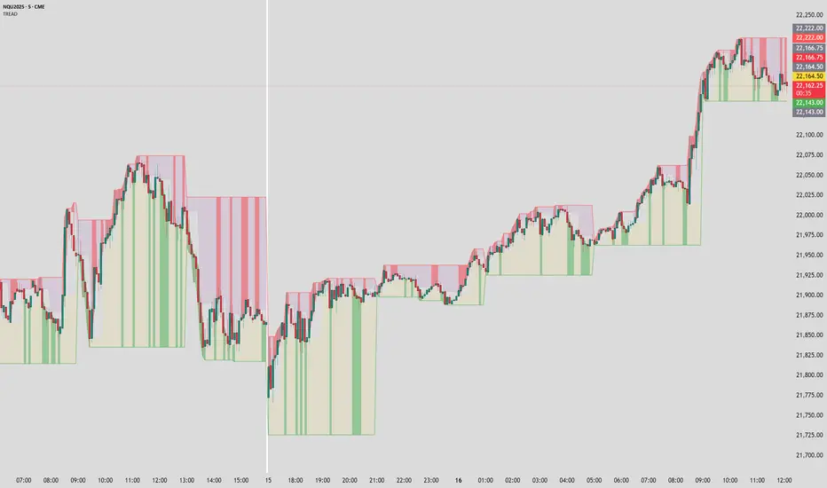
Timeframe Resistance Evaluation And Detection - CoffeeKillerTREAD - Timeframe Resistance Evaluation And Detection Guide
🔔 Important Technical Limitation 🔔
**This indicator does NOT fetch true higher timeframe data.** Instead, it simulates higher timeframe levels by aggregating data from your current chart timeframe. This means:
- Results will vary depending on what chart timeframe you're viewing
- Levels may not match actual higher timeframe candle highs/lows
- You might miss important wicks or gaps that occurred between chart timeframe bars
- **Always verify levels against actual higher timeframe charts before trading**
Welcome traders! This guide will walk you through the TREAD (Timeframe Resistance Evaluation And Detection) indicator, a multi-timeframe analysis tool developed by CoffeeKiller that identifies support and resistance confluence across different time periods.(I am 50+ year old trader and always thought I was bad a teaching and explaining so you get a AI guide. I personally use this on the 5 minute chart with the default settings, but to each there own and if you can improve the trend detection methods please DM me. I would like to see the code. Thanks)
Core Components
1. Dual Timeframe Level Tracking
- Short Timeframe Levels: Tracks opening price extremes within shorter periods
- Long Timeframe Levels: Tracks actual high/low extremes within longer periods
- Dynamic Reset Mechanism: Levels reset at the start of each new timeframe period
- Momentum Detection: Identifies when levels change mid-period, indicating active price movement
2. Visual Zone System
- High Zones: Areas between long timeframe highs and short timeframe highs
- Low Zones: Areas between long timeframe lows and short timeframe lows
- Fill Coloring: Dynamic colors based on whether levels are static or actively changing
- Momentum Highlighting: Special colors when levels break during active periods
3. Customizable Display Options
- Multiple Plot Styles: Line, circles, or cross markers
- Flexible Timeframe Selection: Wide range of short and long timeframe combinations
- Color Customization: Separate colors for each level type and momentum state
- Toggle Controls: Show/hide different elements based on trading preference
Main Features
Timeframe Settings
- Short Timeframe Options: 15m, 30m, 1h, 2h, 4h
- Long Timeframe Options: 1h, 2h, 4h, 8h, 12h, 1D, 1W
- Recommended Combinations:
- Scalping: 15m/1h or 30m/2h
- Day Trading: 30m/4h or 1h/4h
- Swing Trading: 4h/1D or 1D/1W
Display Configuration
- Level Visibility: Toggle short/long timeframe levels independently
- Fill Zone Control: Enable/disable colored zones between levels
- Momentum Fills: Special highlighting for actively changing levels
- Line Customization: Width, style, and color options for all elements
Color System
- Short TF High: Default red for resistance levels
- Short TF Low: Default green for support levels
- Long TF High: Transparent red for broader resistance context
- Long TF Low: Transparent green for broader support context
- Momentum Colors: Brighter colors when levels are actively changing
Technical Implementation Details
How Level Tracking Works
The indicator uses a custom tracking function that:
1. Detects Timeframe Periods: Uses `time()` function to identify when new periods begin
2. Tracks Extremes: Monitors highest/lowest values within each period
3. Resets on New Periods: Clears tracking when timeframe periods change
4. Updates Mid-Period: Continues tracking if new extremes are reached
The Timeframe Limitation Explained
`pinescript
// What the indicator does:
short_tf_start = ta.change(time(short_timeframe)) != 0 // Detects 30m period start
= track_highest(open, short_tf_start) // BUT uses chart TF opens!
// What true multi-timeframe would be:
// short_tf_high = request.security(syminfo.tickerid, short_timeframe, high)
`
This means:
- On a 5m chart with 30m/4h settings: Tracks 5m bar opens during 30m and 4h windows
- On a 1m chart with same settings: Tracks 1m bar opens during 30m and 4h windows
- Results will be different between chart timeframes
- May miss important price action that occurred between your chart's bars
Visual Elements
1. Level Lines
- Short TF High: Upper resistance line from shorter timeframe analysis
- Short TF Low: Lower support line from shorter timeframe analysis
- Long TF High: Broader resistance context from longer timeframe
- Long TF Low: Broader support context from longer timeframe
2. Zone Fills
- High Zone: Area between long TF high and short TF high (potential resistance cluster)
- Low Zone: Area between long TF low and short TF low (potential support cluster)
- Regular Fill: Standard transparency when levels are static
- Momentum Fill: Enhanced visibility when levels are actively changing
3. Dynamic Coloring
- Static Periods: Normal colors when levels haven't changed recently
- Active Periods: Momentum colors when levels are being tested/broken
- Confluence Zones: Different intensities based on timeframe alignment
Trading Applications
1. Support/Resistance Trading
- Entry Points: Trade bounces from zone boundaries
- Confluence Areas: Focus on areas where short and long TF levels cluster
- Zone Breaks: Enter on confirmed breaks through entire zones
- Multiple Timeframe Confirmation: Stronger signals when both timeframes align
2. Range Trading
- Zone Boundaries: Use fill zones as range extremes
- Mean Reversion: Trade back toward opposite zone when price reaches extremes
- Breakout Preparation: Watch for momentum color changes indicating potential breakouts
- Risk Management: Place stops outside the opposite zone
3. Trend Following
- Direction Bias: Trade in direction of zone breaks
- Pullback Entries: Enter on pullbacks to broken zones (now support/resistance)
- Momentum Confirmation: Use momentum coloring to confirm trend strength
- Multiple Timeframe Alignment: Strongest trends when both timeframes agree
4. Scalping Applications
- Quick Bounces: Trade rapid moves between zone boundaries
- Momentum Signals: Enter when momentum colors appear
- Short-Term Targets: Use opposite zone as profit target
- Tight Stops: Place stops just outside current zone
Optimization Guide
1. Timeframe Selection
For Different Trading Styles:
- Scalping: 15m/1h - Quick levels, frequent updates
- Day Trading: 30m/4h - Balanced view, good for intraday moves
- Swing Trading: 4h/1D - Longer-term perspective, fewer false signals
- Position Trading: 1D/1W - Major structural levels
2. Chart Timeframe Considerations
**Important**: Your chart timeframe affects results
- Lower Chart TF: More granular level tracking, but may be noisy
- Higher Chart TF: Smoother levels, but may miss important price action
- Recommended: Use chart timeframe 2-4x smaller than short indicator timeframe
3. Display Settings
- Busy Charts: Disable fills, show only key levels
- Clean Analysis: Enable all fills and momentum coloring
- Multi-Monitor Setup: Use different color schemes for easy identification
- Mobile Trading: Increase line width for visibility
Best Practices
1. Level Verification
- Always Cross-Check: Verify levels against actual higher timeframe charts
- Multiple Timeframes: Check 2-3 different chart timeframes for consistency
- Price Action Confirmation: Wait for candlestick confirmation at levels
- Volume Analysis: Combine with volume for stronger confirmation
2. Risk Management
- Stop Placement: Use zones rather than exact prices for stops
- Position Sizing: Reduce size when zones are narrow (higher risk)
- Multiple Targets: Scale out at different zone boundaries
- False Break Protection: Allow for minor zone penetrations
3. Signal Quality Assessment
- Momentum Colors: Higher probability when momentum coloring appears
- Zone Width: Wider zones often provide stronger support/resistance
- Historical Testing: Backtest on your preferred timeframe combinations
- Market Conditions: Adjust sensitivity based on volatility
Advanced Features
1. Momentum Detection System
The indicator tracks when levels change mid-period:
`pinescript
short_high_changed = short_high != short_high and not short_tf_start
`
This identifies:
- Active level testing
- Potential breakout situations
- Increased market volatility
- Trend acceleration points
2. Dynamic Color System
Complex conditional logic determines fill colors:
- Static Zones: Regular transparency for stable levels
- Active Zones: Enhanced colors for changing levels
- Mixed States: Different combinations based on user preferences
- Custom Overrides: User can prioritize certain color schemes
3. Zone Interaction Analysis
- Convergence: When short and long TF levels approach each other
- Divergence: When timeframes show conflicting levels
- Alignment: When both timeframes agree on direction
- Transition: When one timeframe changes while other remains static
Common Issues and Solutions
1. Inconsistent Levels
Problem: Levels look different on various chart timeframes
Solution: Always verify against actual higher timeframe charts
2. Missing Price Action
Problem: Important wicks or gaps not reflected in levels
Solution: Use chart timeframe closer to indicator's short timeframe setting
3. Too Many Signals
Problem: Excessive level changes and momentum alerts
Solution: Increase timeframe settings or reduce chart timeframe granularity
4. Lagging Signals
Problem: Levels seem to update too slowly
Solution: Decrease chart timeframe or use more sensitive timeframe combinations
Recommended Setups
Conservative Approach
- Timeframes: 4h/1D
- Chart: 1h
- Display: Show fills only, no momentum coloring
- Use: Swing trading, position management
Aggressive Approach
- Timeframes: 15m/1h
- Chart: 5m
- Display: All features enabled, momentum highlighting
- Use: Scalping, quick reversal trades
Balanced Approach
- Timeframes: 30m/4h
- Chart: 15m
- Display: Selective fills, momentum on key levels
- Use: Day trading, multi-session analysis
Final Notes
**Remember**: This indicator provides a synthetic view of multi-timeframe levels, not true higher timeframe data. While useful for identifying potential confluence areas, always verify important levels by checking actual higher timeframe charts.
**Best Results When**:
- Combined with actual multi-timeframe analysis
- Used for confluence confirmation rather than primary signals
- Applied with proper risk management
- Verified against price action and volume
**DISCLAIMER**: This indicator and its signals are intended solely for educational and informational purposes. The timeframe limitation means results may not reflect true higher timeframe levels. Always conduct your own analysis and verify levels independently before making trading decisions. Trading involves significant risk of loss.
Path of Least ResistancePath of Least Resistance (PLR)
Concept Overview
The Path of Least Resistance indicator identifies key zones on your chart that act like "muddy" or "sticky" areas where price tends to get bogged down, creating choppy and unpredictable price action. Between these zones lie the "empty spaces" - clear paths where price can move freely with momentum and direction.
The Analogy: Muddy Fields vs Open Roads
Think of your chart like a landscape:
🟫 ZONES (Muddy/Sticky Areas)
Fair Value Gaps (FVGs) from higher timeframes
Pivot wick zones from higher timeframe pivots
Areas where price gets "stuck" and churns
Like walking through thick mud - slow, choppy, unpredictable movement
Price action becomes erratic and difficult to trade
🟢 EMPTY SPACES (Open Roads)
The clear areas between zones
Where price can move freely with momentum
Like driving on an open highway - smooth, directional movement
The "Path of Least Resistance" for price movement
Trading Philosophy
AVOID Trading Within Zones:
Price action is typically choppy and unpredictable
Higher probability of false signals and whipsaws
Like trying to drive through mud - you'll get stuck
TRADE Through the Empty Spaces:
Look for moves that travel between zones
Price tends to move with momentum and direction
Higher probability setups with cleaner price action
Like taking the highway instead of back roads
Zone Types Detected
Fair Value Gaps (FVGs)
Imbalances from higher timeframe candles
Areas where price "owes" a return visit
Often act as magnets, creating choppy price action
Pivot Wick Zones
Upper and lower wicks from higher timeframe pivots
Rejection areas where price previously struggled
Often create resistance/support that leads to choppy movement
Color Coding System
The zones dynamically change color based on current price position:
🔴 RED ZONES : Price is below the zone (bearish context)
🟢 GREEN ZONES : Price is above the zone (bullish context)
🔘 GRAY ZONES : Price is within the zone (neutral/choppy area)
The "Mum Trades" Strategy
The best trades - what we call "Mum trades" (trades so obvious even your mum could spot them) - happen in the empty spaces between zones:
✅ High Probability Characteristics:
Clear directional movement between zones
Less noise and false signals
Higher momentum and follow-through
Cleaner technical patterns
❌ Avoid These Areas:
Trading within the muddy zones
Expecting clean moves through sticky areas
Fighting against the natural flow of price
Key Features
Auto Timeframe Detection : Automatically selects appropriate higher timeframe
Dynamic Zone Management : Overlapping zones are automatically cleaned up
Real-time Alerts : Get notified when price enters/exits zones
Visual Clarity : Clean zone display with extending boundaries
How to Use
Identify the Zones : Let the indicator mark the muddy areas
Find the Paths : Look for clear spaces between zones
Plan Your Trades : Target moves that travel through empty space
Avoid the Mud : Stay away from trading within the zones
Follow the Flow : Trade with the path of least resistance
Remember
Price, like water, always seeks the path of least resistance. By identifying where that path is clear (empty spaces) versus where it's obstructed (zones), you can align your trading with the natural flow of the market rather than fighting against it.
The goal is simple: Trade the highways, avoid the mud.

Weekend Background Highlighter (UTC+12)## Weekend Background Highlighter (UTC+12)
### Description
This indicator automatically highlights weekend periods on your TradingView charts specifically for the UTC+12 timezone (New Zealand Standard Time). Perfect for traders who need to visualize market closures and weekend gaps in the New Zealand/Pacific time zone, regardless of their exchange's native timezone or chart settings.
### Key Features
- **Fixed UTC+12 Timezone**: Hardcoded to always show weekends according to UTC+12, independent of exchange or chart timezone settings
- **Customizable Appearance**: Adjust background color and opacity to match your chart theme
- **Optional Weekend Labels**: Mark the beginning of each weekend period with customizable labels
- **Debug Mode**: View real-time timezone calculations to verify correct weekend detection
- **Lightweight**: Minimal performance impact with efficient calculations
### Use Cases
- **Forex Traders**: Identify weekend gaps and Monday openings in NZD pairs
- **Cryptocurrency Traders**: Visualize weekend trading patterns in the Pacific timezone
- **Multi-Market Traders**: Maintain consistent weekend awareness across different exchanges
- **Risk Management**: Clearly see when markets are closed for position management
### Settings
- **Weekend Background Color**: Choose any color for the weekend highlight
- **Opacity**: Control transparency (0-100%) to maintain chart visibility
- **Show Weekend Labels**: Toggle labels marking weekend start
- **Debug Info**: Display timezone calculations for verification
### How It Works
The indicator calculates the current UTC time and adds 12 hours to determine the UTC+12 time. It then checks if the resulting day falls on Saturday or Sunday, highlighting these periods on your chart. This ensures weekends are always displayed according to New Zealand time, regardless of your broker's timezone or your local settings.
### Notes
- Weekends begin at 00:00 Saturday UTC+12 (12:00 Friday UTC)
- Weekends end at 00:00 Monday UTC+12 (12:00 Sunday UTC)
- Works on all timeframes and markets
- Compatible with Pine Script v6
### Tags
weekend, background, timezone, UTC+12, New Zealand, highlight, trading sessions, forex, crypto, time zones, market hours, pacific time
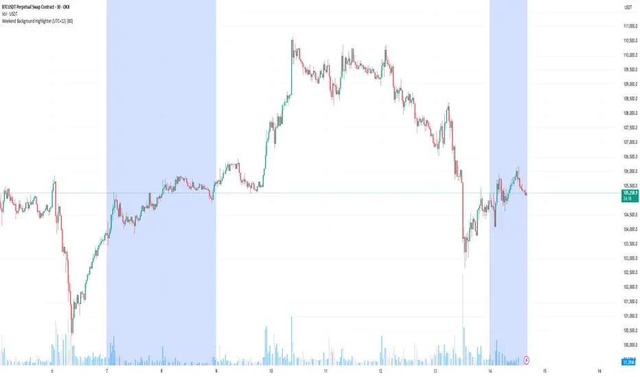
Disguised Candles by The School of Dalal StreetDisguised Candles corrects one of the subtle visual distortions present in normal candlestick charts — the mismatch between the close of one candle and the open of the next.
On many instruments (especially at day/session breaks), the next candle’s open often jumps due to price gaps or data feed behavior. This can make reading the flow of price action harder than necessary.
Disguised Candles fixes this by plotting synthetic candles where the open of each candle is forced to match the close of the previous one — creating a visually continuous flow of price.
Real candles are made fully transparent, so only the "corrected" candles are visible.
This allows traders to:
Visualize price flow as a smooth path
Better spot true directional shifts and trends
Avoid distractions caused by technical gaps that are not meaningful to their strategy
🚀 Pure visual clarity. No noise from false opens.
How it works:
The open of each synthetic candle = close of previous real candle
High, Low, Close remain unchanged
Colors are based on Close vs Corrected Open
Real chart candles are hidden under a transparent overlay
Use this as a clean canvas for trend analysis or as a foundation for building new visual systems.
FvgCalculations█ OVERVIEW
This library provides the core calculation engine for identifying Fair Value Gaps (FVGs) across different timeframes and for processing their interaction with price. It includes functions to detect FVGs on both the current chart and higher timeframes, as well as to check for their full or partial mitigation.
█ CONCEPTS
The library's primary functions revolve around the concept of Fair Value Gaps and their lifecycle.
Fair Value Gap (FVG) Identification
An FVG, or imbalance, represents a price range where buying or selling pressure was significant enough to cause a rapid price movement, leaving an "inefficiency" in the market. This library identifies FVGs based on three-bar patterns:
Bullish FVG: Forms when the low of the current bar (bar 3) is higher than the high of the bar two periods prior (bar 1). The FVG is the space between the high of bar 1 and the low of bar 3.
Bearish FVG: Forms when the high of the current bar (bar 3) is lower than the low of the bar two periods prior (bar 1). The FVG is the space between the low of bar 1 and the high of bar 3.
The library provides distinct functions for detecting FVGs on the current (Low Timeframe - LTF) and specified higher timeframes (Medium Timeframe - MTF / High Timeframe - HTF).
FVG Mitigation
Mitigation refers to price revisiting an FVG.
Full Mitigation: An FVG is considered fully mitigated when price completely closes the gap. For a bullish FVG, this occurs if the current low price moves below or touches the FVG's bottom. For a bearish FVG, it occurs if the current high price moves above or touches the FVG's top.
Partial Mitigation (Entry/Fill): An FVG is partially mitigated when price enters the FVG's range but does not fully close it. The library tracks the extent of this fill. For a bullish FVG, if the current low price enters the FVG from above, that low becomes the new effective top of the remaining FVG. For a bearish FVG, if the current high price enters the FVG from below, that high becomes the new effective bottom of the remaining FVG.
FVG Interaction
This refers to any instance where the current bar's price range (high to low) touches or crosses into the currently unfilled portion of an active (visible and not fully mitigated) FVG.
Multi-Timeframe Data Acquisition
To detect FVGs on higher timeframes, specific historical bar data (high, low, and time of bars at indices and relative to the higher timeframe's last completed bar) is required. The requestMultiTFBarData function is designed to fetch this data efficiently.
█ CALCULATIONS AND USE
The functions in this library are typically used in a sequence to manage FVGs:
1. Data Retrieval (for MTF/HTF FVGs):
Call requestMultiTFBarData() with the desired higher timeframe string (e.g., "60", "D").
This returns a tuple of htfHigh1, htfLow1, htfTime1, htfHigh3, htfLow3, htfTime3.
2. FVG Detection:
For LTF FVGs: Call detectFvg() on each confirmed bar. It uses high , low, low , and high along with barstate.isconfirmed.
For MTF/HTF FVGs: Call detectMultiTFFvg() using the data obtained from requestMultiTFBarData().
Both detection functions return an fvgObject (defined in FvgTypes) if an FVG is found, otherwise na. They also can classify FVGs as "Large Volume" (LV) if classifyLV is true and the FVG size (top - bottom) relative to the tfAtr (Average True Range of the respective timeframe) meets the lvAtrMultiplier.
3. FVG State Updates (on each new bar for existing FVGs):
First, check for overall price interaction using fvgInteractionCheck(). This function determines if the current bar's high/low has touched or entered the FVG's currentTop or currentBottom.
If interaction occurs and the FVG is not already mitigated:
Call checkMitigation() to determine if the FVG has been fully mitigated by the current bar's currentHigh and currentLow. If true, the FVG's isMitigated status is updated.
If not fully mitigated, call checkPartialMitigation() to see if the price has further entered the FVG. This function returns the newLevel to which the FVG has been filled (e.g., currentLow for a bullish FVG, currentHigh for bearish). This newLevel is then used to update the FVG's currentTop or currentBottom.
The calling script (e.g., fvgMain.c) is responsible for storing and managing the array of fvgObject instances and passing them to these update functions.
█ NOTES
Bar State for LTF Detection: The detectFvg() function relies on barstate.isconfirmed to ensure FVG detection is based on closed bars, preventing FVGs from being detected prematurely on the currently forming bar.
Higher Timeframe Data (lookahead): The requestMultiTFBarData() function uses lookahead = barmerge.lookahead_on. This means it can access historical data from the higher timeframe that corresponds to the current bar on the chart, even if the higher timeframe bar has not officially closed. This is standard for multi-timeframe analysis aiming to plot historical HTF data accurately on a lower timeframe chart.
Parameter Typing: Functions like detectMultiTFFvg and detectFvg infer the type for boolean (classifyLV) and numeric (lvAtrMultiplier) parameters passed from the main script, while explicitly typed series parameters (like htfHigh1, currentAtr) expect series data.
fvgObject Dependency: The FVG detection functions return fvgObject instances, and fvgInteractionCheck takes an fvgObject as a parameter. This UDT is defined in the FvgTypes library, making it a dependency for using FvgCalculations.
ATR for LV Classification: The tfAtr (for MTF/HTF) and currentAtr (for LTF) parameters are expected to be the Average True Range values for the respective timeframes. These are used, if classifyLV is enabled, to determine if an FVG's size qualifies it as a "Large Volume" FVG based on the lvAtrMultiplier.
MTF/HTF FVG Appearance Timing: When displaying FVGs from a higher timeframe (MTF/HTF) on a lower timeframe (LTF) chart, users might observe that the most recent MTF/HTF FVG appears one LTF bar later compared to its appearance on a native MTF/HTF chart. This is an expected behavior due to the detection mechanism in `detectMultiTFFvg`. This function uses historical bar data from the MTF/HTF (specifically, data equivalent to `HTF_bar ` and `HTF_bar `) to identify an FVG. Therefore, all three bars forming the FVG on the MTF/HTF must be fully closed and have shifted into these historical index positions relative to the `request.security` call from the LTF chart before the FVG can be detected and displayed on the LTF. This ensures that the MTF/HTF FVG is identified based on confirmed, closed bars from the higher timeframe.
█ EXPORTED FUNCTIONS
requestMultiTFBarData(timeframe)
Requests historical bar data for specific previous bars from a specified higher timeframe.
It fetches H , L , T (for the bar before last) and H , L , T (for the bar three periods prior)
from the requested timeframe.
This is typically used to identify FVG patterns on MTF/HTF.
Parameters:
timeframe (simple string) : The higher timeframe to request data from (e.g., "60" for 1-hour, "D" for Daily).
Returns: A tuple containing: .
- htfHigh1 (series float): High of the bar at index 1 (one bar before the last completed bar on timeframe).
- htfLow1 (series float): Low of the bar at index 1.
- htfTime1 (series int) : Time of the bar at index 1.
- htfHigh3 (series float): High of the bar at index 3 (three bars before the last completed bar on timeframe).
- htfLow3 (series float): Low of the bar at index 3.
- htfTime3 (series int) : Time of the bar at index 3.
detectMultiTFFvg(htfHigh1, htfLow1, htfTime1, htfHigh3, htfLow3, htfTime3, tfAtr, classifyLV, lvAtrMultiplier, tfType)
Detects a Fair Value Gap (FVG) on a higher timeframe (MTF/HTF) using pre-fetched bar data.
Parameters:
htfHigh1 (float) : High of the first relevant bar (typically high ) from the higher timeframe.
htfLow1 (float) : Low of the first relevant bar (typically low ) from the higher timeframe.
htfTime1 (int) : Time of the first relevant bar (typically time ) from the higher timeframe.
htfHigh3 (float) : High of the third relevant bar (typically high ) from the higher timeframe.
htfLow3 (float) : Low of the third relevant bar (typically low ) from the higher timeframe.
htfTime3 (int) : Time of the third relevant bar (typically time ) from the higher timeframe.
tfAtr (float) : ATR value for the higher timeframe, used for Large Volume (LV) FVG classification.
classifyLV (bool) : If true, FVGs will be assessed to see if they qualify as Large Volume.
lvAtrMultiplier (float) : The ATR multiplier used to define if an FVG is Large Volume.
tfType (series tfType enum from no1x/FvgTypes/1) : The timeframe type (e.g., types.tfType.MTF, types.tfType.HTF) of the FVG being detected.
Returns: An fvgObject instance if an FVG is detected, otherwise na.
detectFvg(classifyLV, lvAtrMultiplier, currentAtr)
Detects a Fair Value Gap (FVG) on the current (LTF - Low Timeframe) chart.
Parameters:
classifyLV (bool) : If true, FVGs will be assessed to see if they qualify as Large Volume.
lvAtrMultiplier (float) : The ATR multiplier used to define if an FVG is Large Volume.
currentAtr (float) : ATR value for the current timeframe, used for LV FVG classification.
Returns: An fvgObject instance if an FVG is detected, otherwise na.
checkMitigation(isBullish, fvgTop, fvgBottom, currentHigh, currentLow)
Checks if an FVG has been fully mitigated by the current bar's price action.
Parameters:
isBullish (bool) : True if the FVG being checked is bullish, false if bearish.
fvgTop (float) : The top price level of the FVG.
fvgBottom (float) : The bottom price level of the FVG.
currentHigh (float) : The high price of the current bar.
currentLow (float) : The low price of the current bar.
Returns: True if the FVG is considered fully mitigated, false otherwise.
checkPartialMitigation(isBullish, currentBoxTop, currentBoxBottom, currentHigh, currentLow)
Checks for partial mitigation of an FVG by the current bar's price action.
It determines if the price has entered the FVG and returns the new fill level.
Parameters:
isBullish (bool) : True if the FVG being checked is bullish, false if bearish.
currentBoxTop (float) : The current top of the FVG box (this might have been adjusted by previous partial fills).
currentBoxBottom (float) : The current bottom of the FVG box (similarly, might be adjusted).
currentHigh (float) : The high price of the current bar.
currentLow (float) : The low price of the current bar.
Returns: The new price level to which the FVG has been filled (e.g., currentLow for a bullish FVG).
Returns na if no new partial fill occurred on this bar.
fvgInteractionCheck(fvg, highVal, lowVal)
Checks if the current bar's price interacts with the given FVG.
Interaction means the price touches or crosses into the FVG's
current (possibly partially filled) range.
Parameters:
fvg (fvgObject type from no1x/FvgTypes/1) : The FVG object to check.
Its isMitigated, isVisible, isBullish, currentTop, and currentBottom fields are used.
highVal (float) : The high price of the current bar.
lowVal (float) : The low price of the current bar.
Returns: True if price interacts with the FVG, false otherwise.

Tangent Extrapolation ForecastTangent Extrapolation Forecast
This indicator visually projects price direction by drawing a smoothed sequence of tangent lines based on recent price movements. For each bar in a user-defined lookback window, it calculates the slope over a smoothing period and extends the projected price forward. The resulting polyline forecast connect the endpoints of the extrapolations, and is color-coded to reflect directional changes: green for upward moves, red for downward, and gray for flat segments. This tool can assist traders in visualizing short-term momentum and potential trend continuity without introducing artificial future gaps.
Inputs:
Bars to Use: Number of historical bars used in the forecast.
Slope Smoothing Window: The number of bars used to calculate slope for projection.
Source: Price input for calculations (default is close).
This indicator does not generate buy/sell signals. It is intended as a visual aid to support discretionary analysis.

FVG (Nephew sam remake)Hello i am making my own FVG script inspired by Nephew Sam as his fvg code is not open source. My goal is to replicate his Script and then add in alerts and more functions. Thus, i spent few days trying to code. There is bugs such as lower time frame not showing higher time frame FVG.
This script automatically detects and visualizes Fair Value Gaps (FVGs) — imbalances between demand and supply — across multiple timeframes (15-minute, 1-hour, and 4-hour).
15m chart shows:
15m FVGs (green/red boxes)
1H FVGs (lime/maroon)
4H FVGs (faded green/red with borders) (Bugged For now i only see 1H appearing)
1H chart shows:
1H FVGs
4H FVGs
4H chart shows:
4H FVGs only
There is the function to auto close FVG when a future candle fully disrespected it.
You're welcome to:
🔧 Customize the appearance: adjust box colors, transparency, border style
🧪 Add alerts: e.g., when price enters or fills a gap
📅 Expand to Daily/Weekly: just copy the logic and plug in "D" or "W" as new layers
📈 Build confluence logic: combine this with order blocks, liquidity zones, or ICT concepts
🧠 Experiment with entry signals: e.g., candle confirmation on return to FVG
🚀 Improve performance: if you find a lighter way to track gaps, feel free to optimize!
FVG Candle HighlighterThis indicator highlights only the true Fair Value Gap (FVG) creator candle — the middle candle in a 3-bar FVG formation — with zero clutter.
🔹 Bullish FVG: Candle is colored if price gaps above the high two bars back
🔹 Bearish FVG: Candle is colored if price gaps below the low two bars back
✨ No boxes. No zones. Just pure, visual price-action accuracy.
🔧 Powered by Pine Script v6
🧠 Based on institutional-style FVG logic
🎯 Ideal for Smart Money / ICT / Order Block strategies

UT Bot + Cooldown + Visual FVGSynopsis – UT Bot + Cooldown + Visual FVG
This TradingView script combines:
✅ UT Bot Reversal Signals
Based on ATR and volatility logic
BUY when trend flips from bearish to bullish
SELL when trend flips from bullish to bearish
✅ Cooldown Filter
Limits signals to 1 per X bars (default 30)
Prevents overtrading during choppy price action
✅ Optional FVG Markers (Fair Value Gaps)
Visually shows bullish or bearish imbalances (3-bar gaps)
Does not affect signal generation — only for confluence
🔍 Ideal for traders who want clean, time-filtered signals with visual price-action context. Suitable for futures, crypto, or forex on intraday charts.

Balanced Price Range | Flux Charts💎 GENERAL OVERVIEW
Introducing our new Balanced Price Range (BPR) indicator! A Balanced Price Range is a trading concept used by price action traders. It is detected by finding overlapping area between two contrary Fair Value Gaps (FVGs). These areas can be used as entry points during market pullbacks. For more information about the process, please check the "HOW DOES IT WORK ?" section.
Balanced Price Range Features :
Balanced Price Range Detection : Identifies areas where bullish and bearish FVGs overlap, suggesting a zone of price equilibrium.
Customizable FVG & BPR Detection : You can fine-tune FVG detection and sensitivity for BPR detection to your liking.
Retest Labels : Bullish & Bearish retest labels will be rendered for BPRs.
Alerts : You can set alerts for Bullish & Bearish BPR detection and their retests.
🚩 UNIQUENESS
This indicator doesn't just detect standard FVGs but specifically looks for areas where bullish and bearish IFVGs (Invalidated Fair Value Gaps) overlap, defining a Balanced Price Range. It also actively manages and updates identified BPR zones, removing them when they are invalidated or remain untouched for a specified period. It highlights and alerts users to retests of established BPR zones, signaling potential trading opportunities. Users can tailor the appearance of the BPR zones and retest markers, as well as configure specific alerts for new BPR formations and retests.
📌 HOW DOES IT WORK ?
A Fair Value Gap generally occur when there is an imbalance in the market. They can be detected by specific formations within the chart. The indicator first detects bullish & bearish FVG zones according to their formations on chart. Then, they are dynamically tracked and flagged as invalidated if the price crosses them, turning them into IFVGs. When a FVG & IFVG of the same type overlaps, the indicator combines them into a single BPR of corresponding type. The detected BPR is updated as new data comes in, and renders retests labels as they occur. A bullish BPR can be used to find long trade entry opportunities, while a bearish BPR can be used to find short trade entry opportunities. Retests can also indicate potential movements in the corresponding direction of the BPR. Users can set-up alerts for BPR detection & BPR retests and will get notified as they occur.
⚙️ SETTINGS
Show Historic Zones: If enabled, invalidated or expired BPR zones will remain visible on the chart.
Balanced Price Range:
FVG Detection Method: Determines the criteria for the bar types forming the initial FVG.
Same: All three bars forming the FVG must be of the same type (all bullish or all bearish).
Mixed: The bar types must vary (a mix of bullish and bearish bars).
All: Bar types can vary or be the same.
FVG Invalidation Method: Determines which part of the candle (wick or close) invalidates the initial FVG.
BPR Invalidation Method: Determines which part of the candle (wick or close) invalidates the Balanced Price Range.
Sensitivity: Adjusts the sensitivity of FVG detection. Higher values may identify fewer, larger BPRs, while lower values may detect more, smaller BPRs.
Labels: Toggles the display of text labels on the identified zones.
Retests: Enables or disables the detection and visualization of BPR retests.