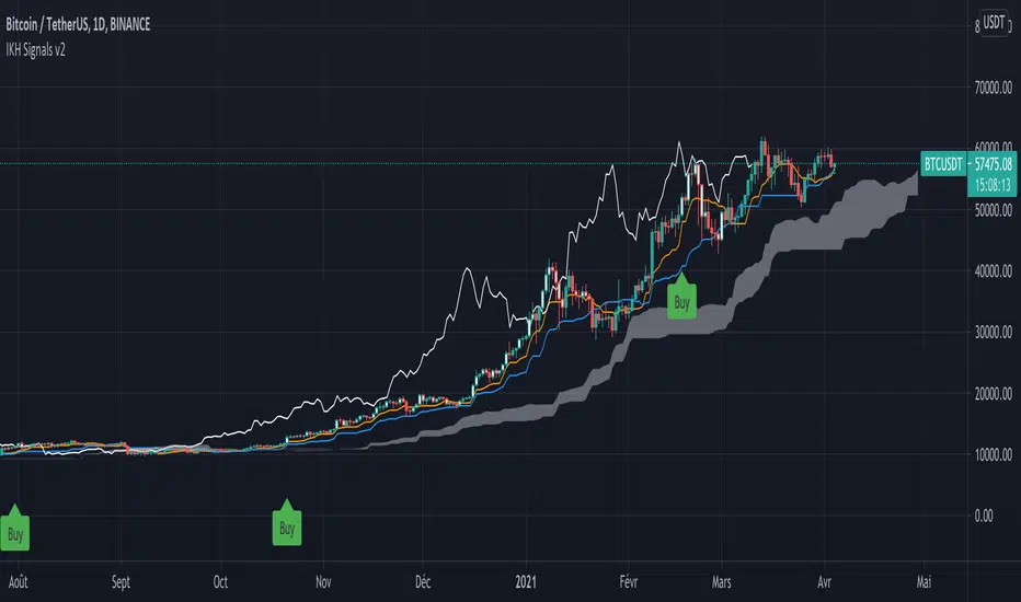
IKH Signals v2Hi,
I'm happy to release this new update after few weeks working.
Fixes
Fix kumo break-out of Chiku span and close price
Fix buy trigger and strong buy trigger
Improvement
Signals take now the kumo thickness and kumo angle
Signals does not trigger on doji candles
Multi time frame validation is now available
I hope this fixes and new features will improve the signals for you too.
Let me know if you find strange behavior or possible improvments.
Cerca negli script per "ichimoku"
【Super Bollinger】The market consists of three phases: an uptrend phase, a downtrend phase, and a range-bound phase.Furthermore, if we include a trend phase and a correction phase, the market has five phases. In other words, the market is classified into the “five phases” as below:
1) Uptrend market (trend phase, upward bias)
2) Downtrend market (trend phase, downward bias)
3) Upward correction phase (correction phase, upward bias)
4) Downward correction phase (correction phase, downward bias)
5) Range-bound phase, sideways (correction phase, basically not biased)
For your judgment of the above market trends, Super Bollinger is extremely useful and effective. And Super Bollinger has advantage in judging market price level.
そもそも、相場は、5つの局面に分けることができます。
すなわち、
1)上昇トレンド局面(上昇バイアス)
2)下降トレンド局面(下降バイアス)
3)調整の反騰局面(上昇バイアス)
4)調整の反落局面(下降バイアス)
5)レンジ局面(バイアスなし)
そして、スーパーボリンジャー、これら5つの局面の判断を下す際にきわめて有効なツールです。また、とりわけ、価格分析に優れたチャートです。
With regard to Chikou Span,this span gives very useful information about (1) the direction of the market (being in an upward bias by buying pressure or in a downward bias by selling pressure) , (2) the timing of buying on the dip or selling on the rally, (3) the market’s temporal rhythm etc..
遅行スパンに関しては、基本的に、
(1)相場の方向性(買い優勢か売り優勢か)
(2)押し目買いや戻り売りのタイミング
(3)相場の時間的リズム
等々に関して実に有効な情報を与えてくれます。
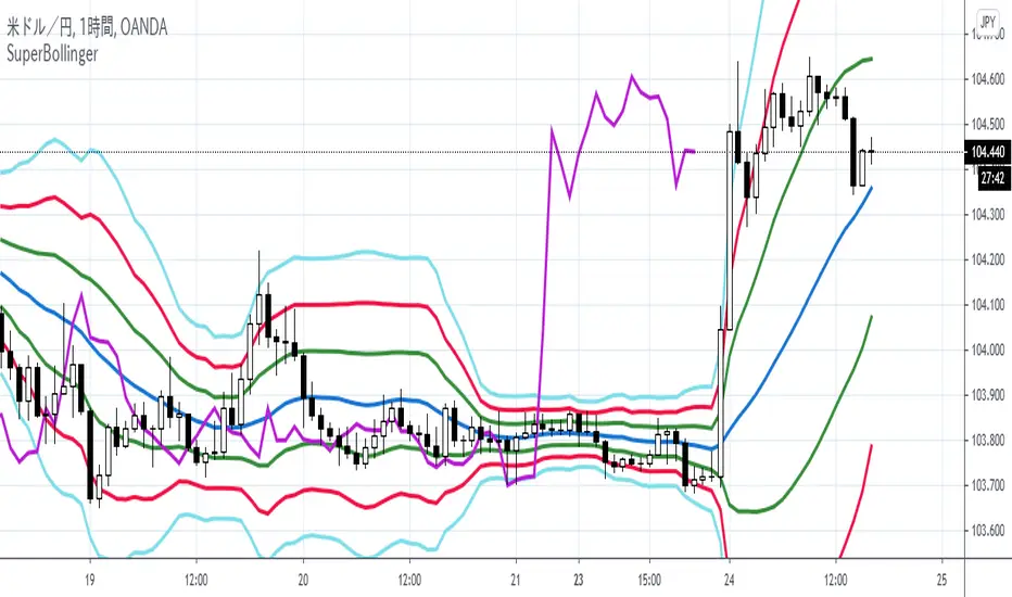
【SpanModel】The Span Model is a very unique chart which shows us especially when to buy and when to sell. And the Span Model has advantage in judging the trade timing.
スパンモデルとは、いつ買うか、いつ売るかを教えてくれるとてもユニークなチャートです。とりわけ、トレードのタイミングを判断する上で優れています。
The Span Model is composed of only three lines (spans).
They are the Blue Span, the Red Span and the Chikou Span.
And a major characteristic of the Span Model is the signals (Span Model Signals) of the two types explained below:
1) Buy signal
The buy signal is lit when the Blue Span sits above, and the Red Span sits below.
2) Sell signal
The sell signal is lit when the Red Span sits above, and the Blue Span sits below.
スパンモデルには、構成要素(3つのスパン)として、青色スパン、赤色スパン、そして、遅行スパンがあります。
スパンモデルの大きな特長として、シグナル(スパンモデルシグナル)があります。そして、2種類のシグナルがあります。
1)買いシグナル
青色スパンが上方、赤色スパンが下方に位置するときに点灯します。
2)売りシグナル
赤色スパンが上方、青色スパンが下方に位置するときに点灯します。

InariN CloudSInariN CloudS (INCS) is my custom model of InariN.
I usually use INCS in 300 ticks (other software) and 5 minutes charts for day trading.
Please read script "InariN simple" for basic usage.
I share background and fundamental ideas of day trading and INCS here.
I start with the practical conclusion and then explain INCS.
Maybe you'll notice that most indicators are unnecessary at the end of this text.
Anyway I compile fundamental ideas that I wanted to know as a beginner.
(I'll update to finish this text, please wait for some time.)
///Premise of trading///
Market's purpose...facilitating trading
Trader's purpose...making money
Market is stronger than trader and trader need adjust to market.
However trader have controllable side.
Market's control...Trend, Volatility
Trader's control...Money management, Making Risk:Reward, Choosing and exercising trading strategy
///Simple rule (Conclusion)///
I made simple rule "Just Do It Now" to check essential ideas on every trade.
Traders can use thousands of indicators but only use three choices "Buy, Sell and No trade".
If you have bad result, you had better suspect not your indicators but your three choices at first.
(This is one of the best advice I have ever heard by N jijii.)

yashi guys
this indicator contain two lines :
the conversion line shifted 17 bar and base line shifted 26 bar
with this indicator u can found where the komo switched and found some potential reversal pivot point
enjoy : Ahmad

Sto RSI and kijun-sen line to determine and follow the trend This script uses 25-75 treshold of stochastic RSI with the help of kijun-sen as confirmation, to find entry points to any trend either newly developed or an established one. I just realized it on the 1 hour SPX chart. Sure it can be used on other symbols. Crossing above/below 25/75 line of sto RSI is considered as buy/sell signal. Signals are evaluated whether price be above/below kijun-sen line. If a sell signal below kijun-sen is generated it is a continuation signal for downtrend, otherwise it is a countertrend signal (maybe a signal for a new downtrend). A countertrend signal must be evaluated carefully and only accepted in the right side of kijun-sen. e.g entering a sell signal generated above kijun-sen should be accepted only below the kijun-sen, vice-versa.

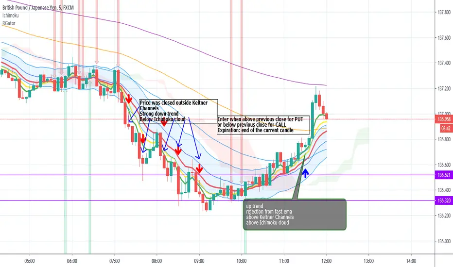
Rainbow Gator - EMAs strategy for Binary OptionThis is an EMAs indicator for Binary Option or Scalping Alert designed for lower Time Frame Trend (2-5minutes).
Although you will find it a useful tool for higher time frames as well.
The Alerts are generated when the fast EMA cross over/under other slower EMAs, you then have the chance to wait for the pullback during the new trend then enter for trend momentum (follow the trend).
Beware when the trend is close to EMA200.
You must draw your SRT (Support-Resistance-Trendline) before looking for setups.
Good luck.
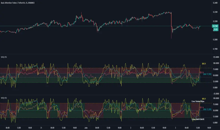
Williams %R + RSI + EMA - [Silver-Wong]
Williams %R + EMA + RSI
Un seul indicateur avec :
- William %R
- RSI
- EMA
- Une ligne médiane
- Les étiquettes des indicateurs
Odin's Kraken (TK Cross Strategy)A simple, yet profitable, trend following system based on 1 hour TK Crosses and ADX.
Works best on ETH/BTC, but is also profitable on other large-cap altcoin BTC pairs (ADA/BTC, EOS/BTC, and TRX/BTC ).
I'm still just getting started in the algo trading world, but if you have any questions I am more than happy to answer them in the comment section here or on Twitter (@pascaltmn).
Cheers.


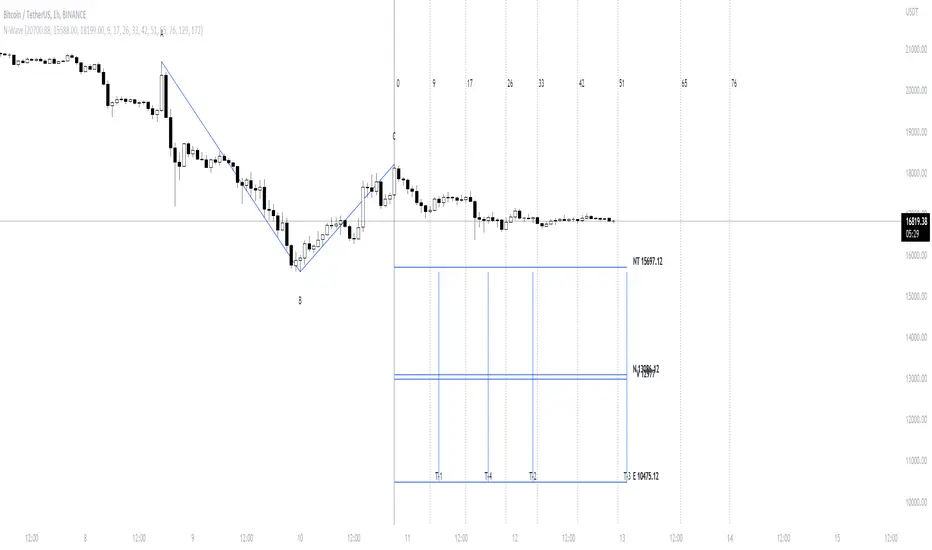
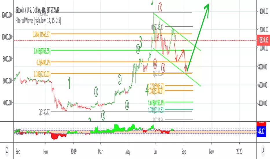
Filtered Waves [NXT2017] #Linda Raschke #basics on Arthur MerrilHI BIG PLAYERS,
this script I wrote for an enquiry of a tradingview-user. It should represent the Filtered Waves idea from Arthur Merril and used by Linda Raschke.
It's similar like a visualization of Elliott Waves.
On YouTube title "MTA UK Chapter Presentation with Linda Raschke" between 34-36 minutes Linda Raschke shows the rules for her Filterd Waves.
Any questions? Ask me!
King regards
NXT2017
========
TO MY PERSON
I'm the second winner of the official German Forex Trading Competition in 2018.
Look here to the ranks:
deutsche-trading-meisterschaften.de
I speak german, english and russian.
My strength in trading are Wolfe Wave pattern.
Bollinger bands/Lagging span crossHello my dear ambitious traders
I'm working hard this week to publish some great indicators this week and open sourced. Hope you'll enjoy, learn and use them.
This will be my greatest reward but comments showing appreciation are also very welcomed (actually likes too) :)
For today, I'll share a simple indicator but it's coming along with some insightful knowledge ^^
Anyway, I'm not here to ask you to this but to share a very cool indicator I made a few months ago and wanted to share for FREE with the community today
The indicator is related to this educational post : What-a-Bollinger-Bands-Lagging-span-cross-can-tell-us/
This trading technique was invented by Robbytrade, a famous french trader twitter.com
I wanted to have those visual signals on the chart so I coded it.
The advantage of being a developer is that you can litteraly code what you miss and get your life better in the process. The one that will find a way to code a new form of money will be rich... wait.... that guy is called Satoshi Nakamoto...
That's all for me today my friends
PS
Trying to update the Trade Manager shared yesterday with some cool features. More to come in the upcoming days
Enjoy
Dave

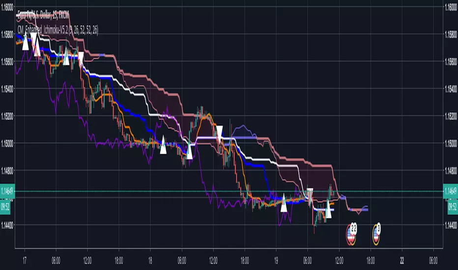
[astropark] Power Tools Overlay//******************************************************************************
// Power Tools Overlay
// Inner Version 1.2.1 13/12/2018
// Developer: iDelphi
// Developer: astropark (Ichimoku Cloud), SMA EMA & Cross tools
//------------------------------------------------------------------------------
// 21/11/2018 Added EMA SMA WMA
// 21/11/2018 Added SMA-EMA EMA-WMA WMA-SMA (Thanks to mariobros1 for the idea of the Simultaneous MA)
// 21/11/2018 Added Bollinger Bands
// 21/11/2018 Added Ichimoku Cloud (Thanks to astropark for all the code of the Ichimoku Cloud)
// 23/11/2018 Show all the indicator as default
// 23/11/2018 Added a cross when single Moving Averages crossing (Thanks to astropark for the idea)
// 24/11/2018 Descriptions Fix
// 24/11/2018 Added Option to enable/disable all Moving Averages
// 10/12/2018 Added EMAs and Crosses
// 13/12/2018 indicator number fixes
//******************************************************************************

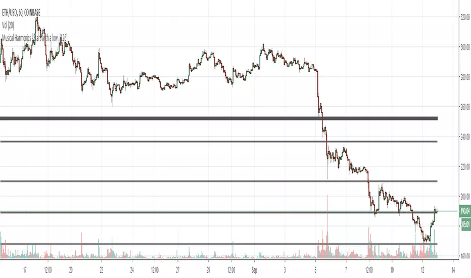
Musical Harmonics - Start with a low.Octaves double from one octave to another, so start with octaves beginning with the number one, for example:
1 doubled is 2, 2 doubled is 4, 4 double is 8 and then we go on to this sequence:
1,2,4,8,16,32,64,126,256,512,1024,2048,etc,etc
Find one of the numbers near a range, so for example on this chart Ethereum was trading at 190.31. That price is in between the octaves of 126 and 256. The number I use as the low for the indicator is 126.
Working on updating with labels and such

2xIchimoku Cloud + 4xEMA + Williams FractalCopy+Pasted/edited the code from :
Moku
www.tradingview.com
EMA
www.tradingview.com
Fractal
www.tradingview.com


vdub Atlasvdub Atlas, Multiple strategy combined indicator
ichmoku,
inside bollinger bands,
Multiple ma's,
Strength indicator MA's
Hull ma,
vdub binaryPro,
Session background colours.
Switch out any indicator you don't want.

Vortex Trend Matrix [JOAT]Vortex Trend Matrix - Multi-Factor Trend Confluence System
Introduction and Purpose
Vortex Trend Matrix is an open-source overlay indicator that combines Ichimoku-style equilibrium analysis with the Vortex Indicator to create a comprehensive trend confluence system. The core problem this indicator solves is that single trend indicators often give conflicting signals. Price might be above a moving average but momentum might be weakening.
This indicator addresses that by combining five different trend factors into a single composite score, making it easy to identify when multiple factors align for high-probability trend trades.
Why These Components Work Together
Each component measures trend from a different perspective:
1. Cloud Position - Price above/below the equilibrium cloud indicates overall trend bias. The cloud acts as dynamic support/resistance.
2. TK Relationship - Conversion line vs Base line (like Tenkan/Kijun in Ichimoku). Conversion above Base = bullish momentum.
3. Lagging Span - Current price compared to price N bars ago. Confirms whether current move has follow-through.
4. Vortex Indicator - VI+ vs VI- measures directional movement strength. Provides momentum confirmation.
5. Base Direction - Whether the base line is rising or falling. Indicates medium-term trend direction.
How the Trend Score Works
float trendScore = 0.0
// Cloud position (+2/-2)
trendScore += aboveCloud ? 2.0 : belowCloud ? -2.0 : 0.0
// TK relationship (+1/-1)
trendScore += conversionLine > baseLine ? 1.0 : conversionLine < baseLine ? -1.0 : 0.0
// Lagging span (+1/-1)
trendScore += laggingBull ? 1.0 : laggingBear ? -1.0 : 0.0
// Vortex (+1.5/-1.5)
trendScore += vortexBull ? 1.5 : vortexBear ? -1.5 : 0.0
// Base direction (+0.5/-0.5)
trendScore += baseDirection * 0.5
Score ranges from approximately -6 to +6:
- +4 or higher = STRONG BULL
- +2 to +4 = BULL
- -2 to +2 = NEUTRAL
- -4 to -2 = BEAR
- -4 or lower = STRONG BEAR
Signal Types
TK Cross Up/Down - Conversion line crosses Base line (momentum shift)
Base Direction Change - Base line changes direction (medium-term shift)
Strong Bull/Bear Trend - Score reaches +4/-4 (high confluence)
Dashboard Information
Trend - Overall status with composite score
Cloud - Price position (ABOVE/BELOW/INSIDE)
TK Cross - Conversion vs Base relationship
Lagging - Lagging span bias
Vortex - VI+/VI- relationship
VI+/VI- - Individual vortex values
How to Use This Indicator
For Trend Following:
1. Enter long when trend score reaches +4 or higher (STRONG BULL)
2. Enter short when trend score reaches -4 or lower (STRONG BEAR)
3. Use cloud as dynamic support/resistance for entries
For Momentum Timing:
1. Watch for TK Cross signals for entry timing
2. Base direction changes indicate medium-term shifts
3. Vortex confirmation adds conviction
For Risk Management:
1. Exit when trend score drops to neutral
2. Use cloud edges as stop-loss references
3. Reduce position when score weakens
Input Parameters
Conversion Period (9) - Fast equilibrium line
Base Period (26) - Slow equilibrium line
Lead Span Period (52) - Cloud projection period
Displacement (26) - Cloud and lagging span offset
Vortex Period (14) - Period for vortex calculation
VI+ Strength (1.10) - Threshold for strong bullish vortex
VI- Strength (0.90) - Threshold for strong bearish vortex
Timeframe Recommendations
4H-Daily: Best for equilibrium-based analysis
1H: Good for intraday trend following
Lower timeframes may require adjusted periods
Limitations
Equilibrium calculations have inherent lag
Cloud displacement means signals are delayed
Works best in trending markets
May whipsaw in ranging conditions
Open-Source and Disclaimer
This script is published as open-source under the Mozilla Public License 2.0 for educational purposes.
This indicator does not constitute financial advice. Trend analysis does not guarantee profitable trades. Always use proper risk management.
- Made with passion by officialjackofalltrades
