HTF Trend FilterTrend filter based on higher timeframe candles. Can be used as entry filters.
Checks if last 3 higher timeframe candles are in fully ascending order or fully descending order. Additionally you can also check if close price is above min of last two highs or below max of last two lows.
Lime and Orange candles imply partial trend in higher timeframe. (only last 3 candles align)
Green and Red candles imply complete trend. (last 3 candles align along with current close price).
Just an experiment. Can be further improved,
Cerca negli script per "order"

Pyramiding Entries On Early Trends (by Coinrule)Pyramiding the entries in a trading strategy may be risky but at the same time very profitable with a proper risk management approach. This strategy seeks to spot early signs of uptrends and increase the position's size while the right conditions persist.
Each trade comes with its stop-loss and take-profit to enforce a proportional risk/reward profile.
The strategy uses a mix of Moving Average based setups to define the buy-signal.
The Moving Average (200) is above the Moving Average (100), which prevents from buying when the uptrend is already in its late stages
The Moving Average (9) is above the Moving Average (100), indicating that the coin is not in a downtrend.
The price crossing above the Moving Average (9) confirms the potential upside used to fire the buy order.
Each entry comes with a stop-loss and a take-profit in a ratio of 1-to-1. After over 400 backtests, we opted for a 3% TP and 3% SL, which provides the best results.
The strategy is optimized on a 1-hour time frame.
The Advantages of this strategy are:
It offers the possibility of adjusting the size of the position proportionally to the confidence in the possibilities that an uptrend will eventually form.
Low drawdowns. On average, the percentage of trades in profit is above 60%, and the stop-loss equal to the take-profit reduces the overall risk.
This strategy returned good returns both with trading pairs with Fiat/stable coins and with BTC. Considering the mixed trends that cryptocurrencies experienced during 2020 vs BTC, this strengthens the strategy's reliability.
The strategy assumes each order to trade 20% of the available capital and pyramids the entries up to 7 times.
A trading fee of 0.1% is taken into account. The fee is aligned to the base fee applied on Binance, which is the largest cryptocurrency exchange.

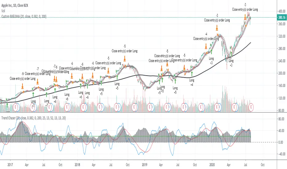
ADX_TSI_Bol Band Trend ChaserThe idea of this script is to be a low risk strategy on trending stocks (or any other trending market), aiming to achieve minimal draw down (e.g. at time of writing AAPL only had ~1.36% draw down, FB ~1.93% draw down and the SPY was 0.80% draw down and all remained profitable).
Testing proved it shouldn't be used in choppy stocks and best period was on daily charts. The back test filter goes back until 2010 so you can obtain 10 years of data.
The strategy utilizes the 200 Moving Average, a Custom Bollinger Band, a TSI with 52 period weighted moving average and ADX strength.
Although back test dates are set to 2010 - 2020, all other filters (moving average, ADX, TSI , Bollinger Band) are not locked so they can be user amended if desired. However the current settings have been tested with manual trading for quite some time to get this combination correct.
Buy signal is given when trading above the 200 moving average + 5 candles have closed above the upper custom Bollinger + the TSI is positive + ADX is above 20.
As back testing proved that this traded better only in tends then some Sell/Short conditions have been removed from the script and this only takes Long orders.
Only requires 2 additional lines of code to add shorting order and then remove the "buy" condition and this could be used for a downward trending stock instead.
Close for either long or short trades is signaled once the TSI crosses in the opposite direction indicating change in trend strength.
Further optimization could be achieved by adding a stop loss, which I may do in the future.
NOTE: This only shows the lower indicators however for visualization you can use my script "CUSTOM BOLLINGER WITH SMA", which is the upper indicators in this strategy.
This is my first attempt at coding a strategy so I'm happy to receive any feedback or hints on how this could be written better from any experienced coders!
NASDAQ:AAPL AMEX:SPY
MMP Indicator 4-step WeeklyFading levels using martingale (limit orders, rebate venue) with no stop-loss orders, long the wings at the end of Support and Resist levels from prior week Friday right before the close. Re-hedge the order book units when there is a breakout.

inwCoin Specific Buy/Sell Price Alert for AutoviewJust simple script to act as conditional stop loss
Problem : Traditional Market Stop or Limit Stop, you have to set it with specific price and wait for the price to drop/pump to your stop then it will trigger. But sometime ( so many times ) the price will leave a very long wick up or down to hunt the stoploss that already set in the exchanges.. then it turn back to the opposite side after stop our position from existent!!
Thank to Autoview, with this simple script, you can setup your "stop level" without put "stop market" in the order.
Just stop when price close below or above specific level in the script, then you can just setup alert to fire the TP/Stop order to exchange via autoview after alert fire.
Example;
You need to stop loss / TP your position when price "close below 9500" in daily BTC chart
- Just set "sell price" to 9500
- and set "Cross down" option
When daily chart close below 9500, the script will trigger alert for you to catch and send to any exchange via Autoview.
Note;
1) When setting alert in tradingview, make sure to use..
- Crossing Down + 0.8 in alert trigger condition
- Set to "Once per bar" ( If you set "once per bar close", it will fire alert in next 2nd candle! )
2) You need to subscribe to autoview to use the bot. And it's not for everyone. Just do your own research before using! ( try to test with small amount of money first! )
Cheers!

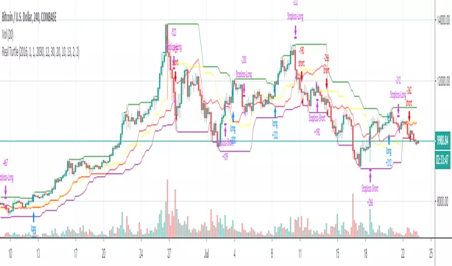
Real TurtleThere are a few different attempts at the turtle strategy on here, but none that I have seen thus far correctly follow the strategy as I know it. This version uses a stop order to trail out of the position by moving the stop order to match the exit channel or stoploss as the N*2( ema of True Range * 2). This version of turtle strategy also uses stop orders for entry on either side in order to enter at optimal time. The ability to specify a backtest period was borrowed from another script, I grabbed it so long ago I no longer remember from whom i borrowed it, if it was yours I will credit you if you PM me.
This version unlike others also allows you to specify a risk % so you only risk that percentage of your equity in a trade, as calculated from your stoploss.
Disclaimer: I have published several scripts in the past when i was first learning pinescript and they are all horrible please ignore those. I would delete them, but TV doesn't allow you to delete.
Alert BatchesThis script lets you separate alerts into batches, and trigger each batch in either sequential order or (pseudo)random order. You can also specify the number of batches being used.
This is helpful when you have alerts to be triggered on every candle, but the number of alerts causes API errors if they are all executed at once.

Glory Hole with SMA + ADX - StrategyHere you get a script with the rules for "Glory Hole"-Strategy from Linda Raschke.
In Addition, I choose the SMA - not the EMA for this script.
MY RECOMMONDATION:
If you get a trade Signal, then set an sell- oder buy-order on the high or low. If the next bar doesn't touch into the trade, then delete your order.
Have fun and good look.

SPY Master v1.0This is a simple swing trading algorithm that uses a fast RSI-EMA to trigger buy/cover signals and a slow RSI-EMA to trigger sell/short signals for SPY, an xchange-traded fund for the S&P 500.
The idea behind this strategy follows the premise that most profitable momentum trades usually occur during periods when price is trending up or down. Periods of flat price actions are usually where most unprofitable trades occur. Because we cannot predict exactly when trending periods will occur, the algorithm basically bets money on all trade opportunities during all market conditions. Despite an accuracy rate of only 40%, the algorithm's asymmetric risk/reward profile allows the average winner to be 2x the average loser. The end result is a positive (profitable) net payout.
TRADING RULES:
Buy/Cover = EMA3(RSI2) cross> 50
Sell/Short = EMA5(RSI2) cross< 50
BACKTEST SETTINGS:
- Period = March 2011 - Present
- Initial capital = $10,000
- Dividends excluded
- Trading costs excluded
PERFORMANCE COMPARISON:
There are 657 trades, which means 1,314 orders. Assuming each order costs $2 (what I pay for at Interactive Brokers), total trading costs should be $2,628.
-SPY (buy & hold) = 132.73 ---> 193.22 = +45.57% (dividends excluded)
-SPY Master v1.0 = $12,649 - $2,628 = $10,021 = +100.21%
DISCLAIMER: None of my ideas and posts are investment advice. Past performance is not an indication of future results. This strategy was constructed with the benefit of hindsight and its future performance cannot be guaranteed.

Ghost BookGhost Book is an indicator that visualizes the distribution of bid and ask amount — the activity of buyers and sellers — in the form of a synthetic order book.
While a real order book shows active limit orders, Ghost Book displays the most recent n ticks (controlled by the input Max rows count in book).
For each tick, the indicator shows:
Price
Amount
Total trade value
Trade side (buyer or seller)
Relative weight of the tick by its amount
The center row displays the current closing price as a reference point between buyers and sellers.
Note: This indicator uses tick-level data. If your TradingView subscription level does not include tick data, the indicator will not function correctly.

Ravi AlgoBot📌 Indicator Description (Publish Notes)
Indicator Name:
EoR / EoS Entry & SL/Target Manager (Put=Red, Call=Green)
Purpose:
यह indicator उन traders के लिए बनाया गया है जो अपनी manual levels (EoR, EoR+1 for Put, और EoS, EoS-1 for Call) को chart पर plot करना चाहते हैं और उनके आधार पर Entry, Stop Loss और Target manage करना चाहते हैं।
How it works:
आप manual prices (EoR, EoR+1, EoS, EoS-1) input fields में डालेंगे।
Put levels (EoR, EoR+1) लाल रंग में दिखेंगे।
Call levels (EoS, EoS-1) हरे रंग में दिखेंगे।
हर price पर chart पर horizontal line + label बनेगा।
आप अपने Stop Loss और Target prices भी manual डाल सकते हैं (Call और Put दोनों के लिए अलग-अलग)।
जब भी price किसी entry/SL/Target level को touch करेगा:
Chart पर signal shape बनेगा (triangle)
एक alertcondition trigger होगा।
आप TradingView में Alerts create करके इन alerts को webhook URL से connect कर सकते हैं।
Example: जब EoR Put level touch हो → webhook के ज़रिए broker/bot में auto order लग जाएगा।
SL और Target levels भी इसी तरह alerts से manage होंगे।
Use Case:
Manual level-based intraday या positional trading
Automated trading setup (via TradingView alerts → Webhook → Broker API)
Put/Call entry, target, SL को clearly visualize और monitor करना
Disclaimer:
यह indicator trading automation tool नहीं है। Actual buy/sell orders Pine Script से नहीं लग सकते। Order execution केवल TradingView Alerts और external webhook के integration से ही possible है। कृपया पहले paper-trade और test करें।

Volume Profile + Pivot Levels [ChartPrime]⯁ OVERVIEW
Volume Profile + Pivot Levels combines a rolling volume profile with price pivots to surface the most meaningful levels in your selected lookback window. It builds a left-side profile from traded volume, highlights the session’s Point of Control (PoC) , and then filters pivot highs/lows so only those aligned with significant profile volume are promoted to chart levels. Each promoted level extends forward until price retests it—so your chart stays focused on levels that actually matter.
⯁ KEY FEATURES
Rolling Volume Profile (Period & Resolution)
Calculates a profile over the last Period bars (default 200). The profile is discretized into Volume Profile Resolution bins (default 50) between the highest high and lowest low inside the window. Each bin accumulates traded volume and is drawn as a smooth left-side polyline for compact, lightweight rendering.
HL = array.new()
// collect highs/lows over 'start' bars to define profile range
for i = 0 to start - 1
HL.push(high ), HL.push(low )
H = HL.max(), L = HL.min()
bin_size = (H - L) / bins
// accumulate per-bin volume
for i = 0 to bins - 1
for j = 0 to start - 1
if close >= (L + bin_sizei) - bin_size and close < (L + bin_size*(i+1)) + bin_size
Bins += volume
Delta-Aware Coloring
The script tracks up-minus-down volume across all period to compute a net Delta . The profile, PoC line, and PoC label adopt a teal tone when net positive, and maroon when net negative—an immediate read on buyer/seller dominance inside the window.
Point of Control (PoC) + Volume Label
Automatically marks the highest-volume bin as the PoC . A horizontal PoC line extends to the last bar, and a label shows the absolute volume at the PoC. Toggle visibility via PoC input.
Pivot Detection with Volume Filter
Identifies raw pivots using Length (default 10) on both sides of the bar. Each candidate pivot is then validated against the profile: only pivots that land within their bin and meet or exceed the Filter % threshold (percentage of PoC volume) are promoted to chart levels. This removes weak, low-participation pivots.
// pivot promotion when volume% >= pivotFilter
if abs(mid - p.value) <= bin_size and volPercent >= pivotFilter
// draw labeled pivot level
line.new(p.index - pivotLength, p.value, p.index + pivotLength, p.value, width = 2)
Forward-Extending, Self-Stopping Levels
Promoted pivot levels extend forward as dotted rays. As soon as price intersects a level (high/low straddles it), that level stops extending—so your chart doesn’t clutter with stale zones.
Concise Level Labels (Volume + %)
Each promoted pivot prints a compact label at the pivot bar with its bin’s absolute volume and percentage of PoC volume (ordering flips for highs vs. lows for quick read).
Lightweight Visuals
The volume profile is rendered as a smooth polyline rather than dozens of boxes, keeping charts responsive even at higher resolutions.
⯁ SETTINGS
Volume Profile → Period : Lookback window used to compute the profile (max 500).
Volume Profile → Resolution : Number of bins; higher = finer structure.
Volume Profile → PoC : Toggle PoC line and volume label.
Pivots → Display : Show/hide volume-validated pivot levels.
Pivots → Length : Pivot detection left/right bars.
Pivots → Filter % 0–100 : Minimum bin strength (as % of PoC) required to promote a pivot level.
⯁ USAGE
Read PoC direction/color for a quick net-flow bias within your window.
Prioritize promoted pivot levels —they’re backed by meaningful participation.
Watch for first retests of promoted levels; the line will stop extending once tested.
Adjust Period / Resolution to match your timeframe (scalps → higher resolution, shorter period; swings → lower resolution, longer period).
Tighten or loosen Filter % to control how selective the level promotion is.
⯁ WHY IT’S UNIQUE
Instead of plotting every pivot or every profile bar, this tool cross-checks pivots against the profile’s internal volume weighting . You only see levels where price structure and liquidity overlap—clean, data-driven levels that self-retire after interaction, so you can focus on what the market actually defends.

Volume Spikes + Daily VWAP SD BandsVolume Spikes + Daily VWAP SD Bands
This indicator combines volume spike detection to help traders identify potential absorption zones with daily VWAP and standard deviation bands , key price levels, continuation opportunities, and possible institutional bias.
Features:
Volume Spike Detection
Highlights candles with unusually high volume relative to a configurable SMA.
Optional filters:
Local highs/lows only (Only Use Valid Highs & Lows)
Candle shapes: Hammer / Shooter only
Candle color match: bullish spikes on green, bearish on red
Plots small circles above/below bars for bullish and bearish volume spikes.
Alerts available for both bullish and bearish spikes.
Interpretation: Volume spikes at local highs/lows can indicate absorption, where one side absorbs aggressive buying/selling pressure.
Daily VWAP
Calculates volume-weighted average price (VWAP) for the current day.
Optionally shows previous day’s VWAP for reference.
Plot lines are customizable with optional circles on lines for visual clarity.
Labels on the last bar show exact VWAP values.
Institutional Bias Insight: Price above both current and previous VWAPs may indicate bullish positioning; price below both VWAPs may indicate bearish positioning. Many professional traders consider this a clue to institutional bias, but it’s not guaranteed. Always confirm with volume, delta, or orderflow analysis.
Standard Deviation Bands
Optional x1 and x2 SD bands around the daily VWAP.
Visual fill between bands shows price volatility zones.
Can be used to identify potential support/resistance or absorption zones.
Use Case: Price bounces off first SD band may indicate continuation signals, especially when volume spikes occur at those levels.
Customizable Visuals
Colors for bullish and bearish volume spikes
VWAP and SD band colors and thickness
Optional circles and filled bands for better readability
Alerts
Bullish / Bearish Volume Spikes
Supports TradingView alert system for automated notifications
Advanced Use Cases:
Combine with Cumulative Delta or Orderflow tools to confirm true absorption zones.
Identify high-volume rejection candles signaling possible trend continuation.
Use VWAP positioning relative to price to assess potential institutional bias, keeping in mind it is probabilistic, not guaranteed.
Visualize intraday VWAP levels and volatility with SD bands for better trade timing.
Settings: Fully customizable, including volume multiplier, SMA length, session filter, candle shape, color options, and VWAP/SD display preferences.

Bracket PreviewThe Bracket Preview indicator allows the user to set their intended bracket order distance (distance, in ticks, to take-profit and stop-loss) from the current live price so that a preview is generated and updated in real-time as price moves. This gives the trader a quick reference of where the bracket orders would be placed if a position were entered at that specific moment in time. This can be helpful by making it more obvious to the trader before a trade is placed exactly where these levels would be in relation to previous price action or if it would be better to wait for price to move to a more favorable level or accept a different Risk-Reward (RR) from this specific trade.
• “If I entered a long position now, would my target be in front of or beyond a recent consolidation area where it is likely to run into resistance and potentially reverse before hitting my take-profit?”
• “Would this bracket order place my stop-loss above or below a previous pivot or would I need to move it after entering the trade and potentially increase the risk on this trade to have it in a more logical level?”
• “If price is in a range and I enter now, would my stop be in the middle of the range while my target is outside the top of the range? Maybe I should wait for price to move to an area where my target would be inside but near the top of the range while my stop loss is below the range so that I’m not taking unnecessary risk or being forced to take an unfavorable RR.”

True Close – Institutional Trading Sessions (Zeiierman)█ Overview
True Close – Institutional Trading Sessions (Zeiierman) is a professional-grade session mapping tool designed to help traders align with how institutions perceive the market’s true close. Unlike the textbook “daily close” used by retail traders, institutional desks often anchor their risk management, execution benchmarks, and exposure metrics to the first hour of the next session.
This indicator visualizes that logic directly on your chart — drawing session boxes, true close levels, and time-aligned labels across Sydney, Tokyo, London, and New York. It highlights the first hour of each session, projects the institutional closing price, and builds a live dashboard that tells you which sessions are active, which are in the critical opening phase, and what levels matter most right now.
More than just a visual tool, this indicator embeds institutional rhythm directly into your workflow — giving you a window into where big players finalize yesterday’s business, rebalance exposure, and execute delayed orders. It’s not just about painting sessions on your chart — it’s about adopting the mindset of those who truly move the market. Institutions don’t settle risk at the bell; they complete it in the next session. This tool lets you see that transition in real time, giving you an edge that goes beyond candles and indicators.
█ How It Works
⚪ Session Detection Engine
Each session is identified by its own time block (e.g., 09:00–17:30 for London). Once a session opens:
A full-session box is drawn to track its range.
The first hour is highlighted separately.
Once the first hour completes, the true close line is plotted, representing the price institutions often treat as the "real" close of the prior day.
⚪ Institutional True Close Logic
The script captures the close of the first hour, not the end of the day.
This line becomes a static reference across your chart, letting you visualize how price interacts with that institutional anchor:
Rejections from it show where yesterday's flow is respected.
Breaks through it may indicate that today's flows are rewriting the narrative.
⚪ Dynamic Dashboard Table
A live table appears in the corner of your screen, showing:
Each session's active status
Whether we’re inside the first hour
The current “true close” price if available
Each cell comes with advanced tooltips giving institutional context, flow dynamics, and market microstructure insights — from rebalancing spillovers to VWAP/TWAP lag effects.
█ How to Use
⚪ Use the First-Hour Line as Your Institutional Anchor
Treat it like the price level that big funds care about. Watch how the price behaves around level. Fades, re-tests, or continuation moves often occur as the market finishes recapping yesterday’s leftover orders.
⚪ Structure Entries Around the Session Context
Are you inside the first hour? Expect more volatility, more decisive flow. After the first session hour, expect fading liquidity as the market slows down and awaits the next session to open.
█ Settings
UTC Offset – Select your preferred time zone; all sessions adjust accordingly.
Session Toggles – Enable/disable Sydney, Tokyo, London, or NY.
Box Display Options – Show/hide session background, first-hour fill, borders.
True Close Line Controls – Enable line, label, and customize width & color.
Execution Hour Labels – Optional toggle for first-hour label placement.
-----------------
Disclaimer
The content provided in my scripts, indicators, ideas, algorithms, and systems is for educational and informational purposes only. It does not constitute financial advice, investment recommendations, or a solicitation to buy or sell any financial instruments. I will not accept liability for any loss or damage, including without limitation any loss of profit, which may arise directly or indirectly from the use of or reliance on such information.
All investments involve risk, and the past performance of a security, industry, sector, market, financial product, trading strategy, backtest, or individual's trading does not guarantee future results or returns. Investors are fully responsible for any investment decisions they make. Such decisions should be based solely on an evaluation of their financial circumstances, investment objectives, risk tolerance, and liquidity needs.

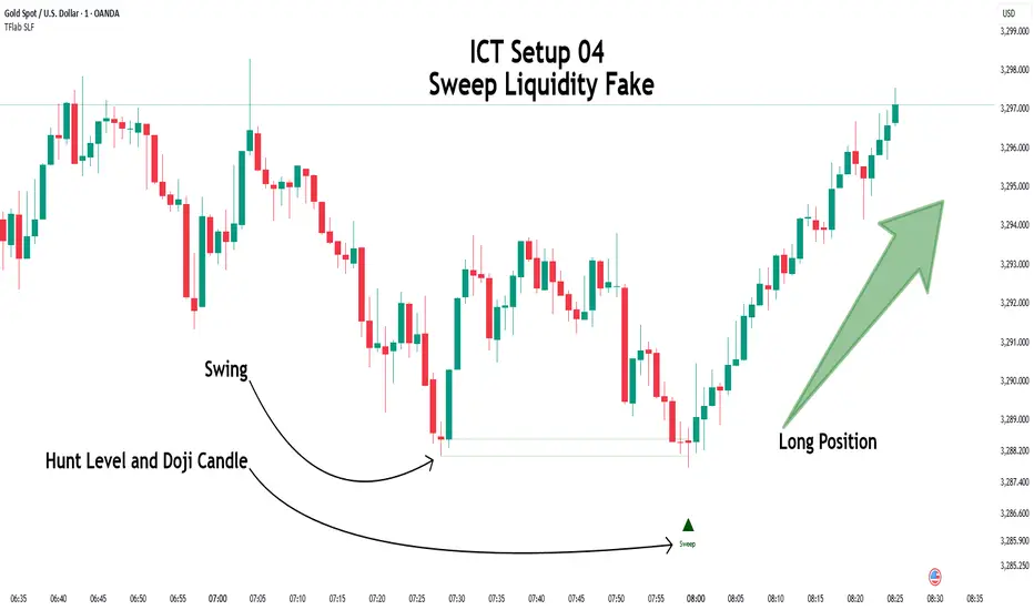
ICT Setup 04 [TradingFinder] SFP Sweep Liquidity Fake CHoCH/BOS🔵 Introduction
In smart money and ICT based trading, liquidity is never random. Some of the most meaningful market moves begin with a liquidity sweep where price intentionally hunts a previous swing high or swing low to trigger stop loss orders and absorb volume.
This manipulation is often followed by a sharp reversal from a reaction zone, creating ideal conditions for a high probability entry. This indicator is built to detect exactly that. It identifies a valid swing point and defines a reaction zone where price is likely to react.
For short setups, the zone lies between the swing high and the maximum of the candle’s open or close. For long setups, it’s drawn from the swing low to the minimum of the open or close.
When price returns to this zone and forms a qualified confirmation candle typically a doji or a small bodied candle that closes inside the zone while sweeping the liquidity this is a potential sign of reversal.
The candle must show both the sweep and the inability to hold above or below the key level, signaling a fake breakout or failed move. By combining elements of liquidity hunt, reaction zone rejection, and candle based entry confirmation, this tool highlights sniper entry points used by smart money to trap retail traders and reverse the trend. It helps filter out noise and enhances timing, making it ideal for trading in alignment with institutional order flow.
Long Position :
Short Position :
🔵 How to Use
This indicator is designed to highlight precise moments where price sweeps liquidity and reacts within a high probability reversal zone. By identifying clean swing highs and lows and defining a smart reaction zone around them, it filters out weak fakeouts and focuses only on setups with strong institutional footprints.
The tool works best when combined with market structure analysis and is suitable for both scalping and intraday trading. Below is a breakdown of how to interpret the signals for long and short positions based on the visual setups provided.
🟣 Long Setup
In a long setup, the indicator first detects a valid swing low where liquidity has likely accumulated below. A reaction zone is then drawn between the swing low and the minimum of the open or close of the swing candle.
When price returns to this zone, it must sweep the previous low and form a precise confirmation candle, such as a doji or a small bodied candle, that closes inside the zone. This candle must also reject the lower level, showing failure to continue downward.
As shown in the chart, once the liquidity grab is complete and the confirmation candle forms, a clean long signal is issued, indicating a potential bullish reversal backed by smart money behavior.
🟣 Short Setup
In a short setup, the indicator identifies a swing high where buy-side liquidity is resting. It then constructs a reaction zone between the high and the maximum of the open or close of the swing candle. Price must return to this zone, sweep the swing high, and form a bearish confirmation candle inside the zone.
A classic example is a doji or rejection candle that traps breakout buyers and fails to hold above the previous high. In the provided chart, the price aggressively hunts the liquidity above the swing high, but the close within the reaction zone signals exhaustion, prompting a short signal with high reversal probability.
These setups represent moments where price action, liquidity behavior, and candle structure align to offer strong entries. By focusing on clean sweeps and reactive confirmations, the indicator helps traders stay on the side of smart money and avoid common breakout traps.
🔵 Settings
🟣 Logical settings
Swing period : You can set the swing detection period.
Max Swing Back Method : It is in two modes "All" and "Custom". If it is in "All" mode, it will check all swings, and if it is in "Custom" mode, it will check the swings to the extent you determine.
Max Swing Back : You can set the number of swings that will go back for checking.
Maximum Distance Between Swing and Signal :The maximum number of candles allowed between the swing point and the potential signal. The default value is 50, ensuring that only recent and relevant price reactions are considered valid.
🟣 Display settings
Displaying or not displaying swings and setting the color of labels and lines.
🟣 Alert Settings
Alert SFP : Enables alerts for Swing Failure Pattern.
Message Frequency : Determines the frequency of alerts. Options include 'All' (every function call), 'Once Per Bar' (first call within the bar), and 'Once Per Bar Close' (final script execution of the real-time bar). Default is 'Once per Bar'.
Show Alert Time by Time Zone : Configures the time zone for alert messages. Default is 'UTC'.
🔵 Conclusion
This indicator is built for traders who rely on liquidity driven setups and smart money principles. By combining swing structure analysis with precision reaction zones and strict entry confirmation, it isolates the exact moments where price sweeps liquidity and fails to continue. These are high value points where institutional activity often reveals itself, and retail traps unfold.
Unlike generic breakout tools, this script focuses on quality over quantity by requiring both a sweep of a swing high or low and a confirmed rejection candle that closes inside a predefined zone. With customizable swing depth, proximity filters, visual highlights, and alert functions, it offers a complete framework for identifying and acting on fake breakouts with confidence. Whether you trade forex, crypto, or indices, this tool enhances your ability to align with true order flow and take entries where liquidity is most likely to shift.
Multi-Position DashMulti-Position Dash — Risk Dashboard for Forex, Stocks & Indices
Overview:
The Multi-Position Dash is a highly customizable trading dashboard designed to help active traders manage up to 8 simultaneous positions across Forex, Stocks, and Indices. Whether you're trading single entries, layering positions, using DCA (Dollar Cost Averaging), or running complex hedging setups, this tool provides essential, real-time risk and P&L insights—directly on your chart.
Key Features:
✔️ Supports Forex, Stocks, Indices — with automatic pip and contract conversions
✔️ Track up to 8 manual positions, each with customizable direction, lot size or contracts, entry price, Take Profit, and Stop Loss
✔️ Full GBP-based P&L and risk calculation, including automatic USD-to-GBP conversion for non-FX assets
✔️ Real-time display of:
Total potential Take Profit (GBP)
Total potential Stop Loss (GBP)
Risk % relative to account balance
Live P&L (GBP) based on current price
✔️ Breakeven price calculation, even across mixed-direction positions (DCA & hedging aware)
✔️ Visual breakeven line, live P&L arrows, and entry price markers
✔️ Shared Stop Loss option for all positions — perfect for DCA traders
✔️ Easy export strings for logging trades to external tools like spreadsheets
Ideal For:
✅ Forex traders using lot-based risk models
✅ Stock & Index traders wanting simplified contract-based position tracking
✅ Traders managing multiple active positions, with or without hedging
✅ Anyone needing at-a-glance P&L and risk monitoring, independent of broker platforms
Notes & Usage:
This is a manual tracking tool—you enter your positions, TP, SL levels, etc., and the dashboard calculates the rest. It does not place or manage live orders.
Supports both Long and Short positions.
All calculations are based on your inputs and market price—accuracy depends on maintaining your inputs properly.
Shared Stop Loss feature applies a single, unified stop across all active positions for simplified risk control in DCA setups.
GBP is used as the account currency—USD-to-GBP conversion is applied to stocks and indices as needed.
Disclaimer:
This tool is for educational and planning purposes only. It does not place or manage live trades, and is not a substitute for broker risk management tools. Always double-check your own position sizing and risk before placing live orders.

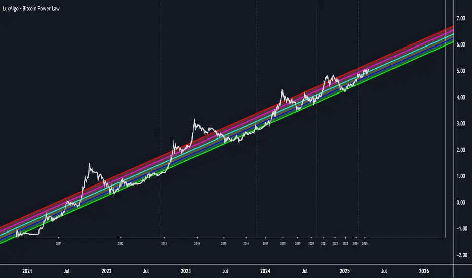
Bitcoin Power Law [LuxAlgo]The Bitcoin Power Law tool is a representation of Bitcoin prices first proposed by Giovanni Santostasi, Ph.D. It plots BTCUSD daily closes on a log10-log10 scale, and fits a linear regression channel to the data.
This channel helps traders visualise when the price is historically in a zone prone to tops or located within a discounted zone subject to future growth.
🔶 USAGE
Giovanni Santostasi, Ph.D. originated the Bitcoin Power-Law Theory; this implementation places it directly on a TradingView chart. The white line shows the daily closing price, while the cyan line is the best-fit regression.
A channel is constructed from the linear fit root mean squared error (RMSE), we can observe how price has repeatedly oscillated between each channel areas through every bull-bear cycle.
Excursions into the upper channel area can be followed by price surges and finishing on a top, whereas price touching the lower channel area coincides with a cycle low.
Users can change the channel areas multipliers, helping capture moves more precisely depending on the intended usage.
This tool only works on the daily BTCUSD chart. Ticker and timeframe must match exactly for the calculations to remain valid.
🔹 Linear Scale
Users can toggle on a linear scale for the time axis, in order to obtain a higher resolution of the price, (this will affect the linear regression channel fit, making it look poorer).
🔶 DETAILS
One of the advantages of the Power Law Theory proposed by Giovanni Santostasi is its ability to explain multiple behaviors of Bitcoin. We describe some key points below.
🔹 Power-Law Overview
A power law has the form y = A·xⁿ , and Bitcoin’s key variables follow this pattern across many orders of magnitude. Empirically, price rises roughly with t⁶, hash-rate with t¹² and the number of active addresses with t³.
When we plot these on log-log axes they appear as straight lines, revealing a scale-invariant system whose behaviour repeats proportionally as it grows.
🔹 Feedback-Loop Dynamics
Growth begins with new users, whose presence pushes the price higher via a Metcalfe-style square-law. A richer price pool funds more mining hardware; the Difficulty Adjustment immediately raises the hash-rate requirement, keeping profit margins razor-thin.
A higher hash rate secures the network, which in turn attracts the next wave of users. Because risk and Difficulty act as braking forces, user adoption advances as a power of three in time rather than an unchecked S-curve. This circular causality repeats without end, producing the familiar boom-and-bust cadence around the long-term power-law channel.
🔹 Scale Invariance & Predictions
Scale invariance means that enlarging the timeline in log-log space leaves the trajectory unchanged.
The same geometric proportions that described the first dollar of value can therefore extend to a projected million-dollar bitcoin, provided no catastrophic break occurs. Institutional ETF inflows supply fresh capital but do not bend the underlying slope; only a persistent deviation from the line would falsify the current model.
🔹 Implications
The theory assigns scarcity no direct role; iterative feedback and the Difficulty Adjustment are sufficient to govern Bitcoin’s expansion. Long-term valuation should focus on position within the power-law channel, while bubbles—sharp departures above trend that later revert—are expected punctuations of an otherwise steady climb.
Beyond about 2040, disruptive technological shifts could alter the parameters, but for the next order of magnitude the present slope remains the simplest, most robust guide.
Bitcoin behaves less like a traditional asset and more like a self-organising digital organism whose value, security, and adoption co-evolve according to immutable power-law rules.
🔶 SETTINGS
🔹 General
Start Calculation: Determine the start date used by the calculation, with any prior prices being ignored. (default - 15 Jul 2010)
Use Linear Scale for X-Axis: Convert the horizontal axis from log(time) to linear calendar time
🔹 Linear Regression
Show Regression Line: Enable/disable the central power-law trend line
Regression Line Color: Choose the colour of the regression line
Mult 1: Toggle line & fill, set multiplier (default +1), pick line colour and area fill colour
Mult 2: Toggle line & fill, set multiplier (default +0.5), pick line colour and area fill colour
Mult 3: Toggle line & fill, set multiplier (default -0.5), pick line colour and area fill colour
Mult 4: Toggle line & fill, set multiplier (default -1), pick line colour and area fill colour
🔹 Style
Price Line Color: Select the colour of the BTC price plot
Auto Color: Automatically choose the best contrast colour for the price line
Price Line Width: Set the thickness of the price line (1 – 5 px)
Show Halvings: Enable/disable dotted vertical lines at each Bitcoin halving
Halvings Color: Choose the colour of the halving lines
Why EMA Isn't What You Think It IsMany new traders adopt the Exponential Moving Average (EMA) believing it's simply a "better Simple Moving Average (SMA)". This common misconception leads to fundamental misunderstandings about how EMA works and when to use it.
EMA and SMA differ at their core. SMA use a window of finite number of data points, giving equal weight to each data point in the calculation period. This makes SMA a Finite Impulse Response (FIR) filter in signal processing terms. Remember that FIR means that "all that we need is the 'period' number of data points" to calculate the filter value. Anything beyond the given period is not relevant to FIR filters – much like how a security camera with 14-day storage automatically overwrites older footage, making last month's activity completely invisible regardless of how important it might have been.
EMA, however, is an Infinite Impulse Response (IIR) filter. It uses ALL historical data, with each past price having a diminishing - but never zero - influence on the calculated value. This creates an EMA response that extends infinitely into the past—not just for the last N periods. IIR filters cannot be precise if we give them only a 'period' number of data to work on - they will be off-target significantly due to lack of context, like trying to understand Game of Thrones by watching only the final season and wondering why everyone's so upset about that dragon lady going full pyromaniac.
If we only consider a number of data points equal to the EMA's period, we are capturing no more than 86.5% of the total weight of the EMA calculation. Relying on he period window alone (the warm-up period) will provide only 1 - (1 / e^2) weights, which is approximately 1−0.1353 = 0.8647 = 86.5%. That's like claiming you've read a book when you've skipped the first few chapters – technically, you got most of it, but you probably miss some crucial early context.
▶️ What is period in EMA used for?
What does a period parameter really mean for EMA? When we select a 15-period EMA, we're not selecting a window of 15 data points as with an SMA. Instead, we are using that number to calculate a decay factor (α) that determines how quickly older data loses influence in EMA result. Every trader knows EMA calculation: α = 1 / (1+period) – or at least every trader claims to know this while secretly checking the formula when they need it.
Thinking in terms of "period" seriously restricts EMA. The α parameter can be - should be! - any value between 0.0 and 1.0, offering infinite tuning possibilities of the indicator. When we limit ourselves to whole-number periods that we use in FIR indicators, we can only access a small subset of possible IIR calculations – it's like having access to the entire RGB color spectrum with 16.7 million possible colors but stubbornly sticking to the 8 basic crayons in a child's first art set because the coloring book only mentioned those by name.
For example:
Period 10 → alpha = 0.1818
Period 11 → alpha = 0.1667
What about wanting an alpha of 0.17, which might yield superior returns in your strategy that uses EMA? No whole-number period can provide this! Direct α parameterization offers more precision, much like how an analog tuner lets you find the perfect radio frequency while digital presets force you to choose only from predetermined stations, potentially missing the clearest signal sitting right between channels.
Sidenote: the choice of α = 1 / (1+period) is just a convention from 1970s, probably started by J. Welles Wilder, who popularized the use of the 14-day EMA. It was designed to create an approximate equivalence between EMA and SMA over the same number of periods, even thought SMA needs a period window (as it is FIR filter) and EMA doesn't. In reality, the decay factor α in EMA should be allowed any valye between 0.0 and 1.0, not just some discrete values derived from an integer-based period! Algorithmic systems should find the best α decay for EMA directly, allowing the system to fine-tune at will and not through conversion of integer period to float α decay – though this might put a few traditionalist traders into early retirement. Well, to prevent that, most traditionalist implementations of EMA only use period and no alpha at all. Heaven forbid we disturb people who print their charts on paper, draw trendlines with rulers, and insist the market "feels different" since computers do algotrading!
▶️ Calculating EMAs Efficiently
The standard textbook formula for EMA is:
EMA = CurrentPrice × alpha + PreviousEMA × (1 - alpha)
But did you know that a more efficient version exists, once you apply a tiny bit of high school algebra:
EMA = alpha × (CurrentPrice - PreviousEMA) + PreviousEMA
The first one requires three operations: 2 multiplications + 1 addition. The second one also requires three ops: 1 multiplication + 1 addition + 1 subtraction.
That's pathetic, you say? Not worth implementing? In most computational models, multiplications cost much more than additions/subtractions – much like how ordering dessert costs more than asking for a water refill at restaurants.
Relative CPU cost of float operations :
Addition/Subtraction: ~1 cycle
Multiplication: ~5 cycles (depending on precision and architecture)
Now you see the difference? 2 * 5 + 1 = 11 against 5 + 1 + 1 = 7. That is ≈ 36.36% efficiency gain just by swapping formulas around! And making your high school math teacher proud enough to finally put your test on the refrigerator.
▶️ The Warmup Problem: how to start the EMA sequence right
How do we calculate the first EMA value when there's no previous EMA available? Let's see some possible options used throughout the history:
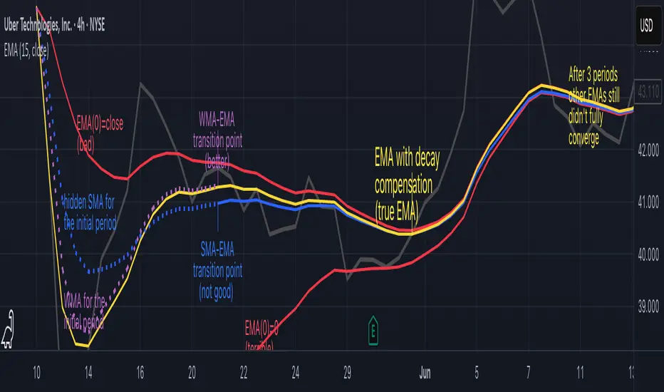
Start with zero : EMA(0) = 0. This creates stupidly large distortion until enough bars pass for the horrible effect to diminish – like starting a trading account with zero balance but backdating a year of missed trades, then watching your balance struggle to climb out of a phantom debt for months.
Start with first price : EMA(0) = first price. This is better than starting with zero, but still causes initial distortion that will be extra-bad if the first price is an outlier – like forming your entire opinion of a stock based solely on its IPO day price, then wondering why your model is tanking for weeks afterward.
Use SMA for warmup : This is the tradition from the pencil-and-paper era of technical analysis – when calculators were luxury items and "algorithmic trading" meant your broker had neat handwriting. We first calculate an SMA over the initial period, then kickstart the EMA with this average value. It's widely used due to tradition, not merit, creating a mathematical Frankenstein that uses an FIR filter (SMA) during the initial period before abruptly switching to an IIR filter (EMA). This methodology is so aesthetically offensive (abrupt kink on the transition from SMA to EMA) that charting platforms hide these early values entirely, pretending EMA simply doesn't exist until the warmup period passes – the technical analysis equivalent of sweeping dust under the rug.
Use WMA for warmup : This one was never popular because it is harder to calculate with a pencil - compared to using simple SMA for warmup. Weighted Moving Average provides a much better approximation of a starting value as its linear descending profile is much closer to the EMA's decay profile.
These methods all share one problem: they produce inaccurate initial values that traders often hide or discard, much like how hedge funds conveniently report awesome performance "since strategy inception" only after their disastrous first quarter has been surgically removed from the track record.
▶️ A Better Way to start EMA: Decaying compensation
Think of it this way: An ideal EMA uses an infinite history of prices, but we only have data starting from a specific point. This creates a problem - our EMA starts with an incorrect assumption that all previous prices were all zero, all close, or all average – like trying to write someone's biography but only having information about their life since last Tuesday.
But there is a better way. It requires more than high school math comprehension and is more computationally intensive, but is mathematically correct and numerically stable. This approach involves compensating calculated EMA values for the "phantom data" that would have existed before our first price point.
Here's how phantom data compensation works:
We start our normal EMA calculation:
EMA_today = EMA_yesterday + α × (Price_today - EMA_yesterday)
But we add a correction factor that adjusts for the missing history:
Correction = 1 at the start
Correction = Correction × (1-α) after each calculation
We then apply this correction:
True_EMA = Raw_EMA / (1-Correction)
This correction factor starts at 1 (full compensation effect) and gets exponentially smaller with each new price bar. After enough data points, the correction becomes so small (i.e., below 0.0000000001) that we can stop applying it as it is no longer relevant.
Let's see how this works in practice:
For the first price bar:
Raw_EMA = 0
Correction = 1
True_EMA = Price (since 0 ÷ (1-1) is undefined, we use the first price)
For the second price bar:
Raw_EMA = α × (Price_2 - 0) + 0 = α × Price_2
Correction = 1 × (1-α) = (1-α)
True_EMA = α × Price_2 ÷ (1-(1-α)) = Price_2
For the third price bar:
Raw_EMA updates using the standard formula
Correction = (1-α) × (1-α) = (1-α)²
True_EMA = Raw_EMA ÷ (1-(1-α)²)
With each new price, the correction factor shrinks exponentially. After about -log₁₀(1e-10)/log₁₀(1-α) bars, the correction becomes negligible, and our EMA calculation matches what we would get if we had infinite historical data.
This approach provides accurate EMA values from the very first calculation. There's no need to use SMA for warmup or discard early values before output converges - EMA is mathematically correct from first value, ready to party without the awkward warmup phase.
Here is Pine Script 6 implementation of EMA that can take alpha parameter directly (or period if desired), returns valid values from the start, is resilient to dirty input values, uses decaying compensator instead of SMA, and uses the least amount of computational cycles possible.
// Enhanced EMA function with proper initialization and efficient calculation
ema(series float source, simple int period=0, simple float alpha=0)=>
// Input validation - one of alpha or period must be provided
if alpha<=0 and period<=0
runtime.error("Alpha or period must be provided")
// Calculate alpha from period if alpha not directly specified
float a = alpha > 0 ? alpha : 2.0 / math.max(period, 1)
// Initialize variables for EMA calculation
var float ema = na // Stores raw EMA value
var float result = na // Stores final corrected EMA
var float e = 1.0 // Decay compensation factor
var bool warmup = true // Flag for warmup phase
if not na(source)
if na(ema)
// First value case - initialize EMA to zero
// (we'll correct this immediately with the compensation)
ema := 0
result := source
else
// Standard EMA calculation (optimized formula)
ema := a * (source - ema) + ema
if warmup
// During warmup phase, apply decay compensation
e *= (1-a) // Update decay factor
float c = 1.0 / (1.0 - e) // Calculate correction multiplier
result := c * ema // Apply correction
// Stop warmup phase when correction becomes negligible
if e <= 1e-10
warmup := false
else
// After warmup, EMA operates without correction
result := ema
result // Return the properly compensated EMA value
▶️ CONCLUSION
EMA isn't just a "better SMA"—it is a fundamentally different tool, like how a submarine differs from a sailboat – both float, but the similarities end there. EMA responds to inputs differently, weighs historical data differently, and requires different initialization techniques.
By understanding these differences, traders can make more informed decisions about when and how to use EMA in trading strategies. And as EMA is embedded in so many other complex and compound indicators and strategies, if system uses tainted and inferior EMA calculatiomn, it is doing a disservice to all derivative indicators too – like building a skyscraper on a foundation of Jell-O.
The next time you add an EMA to your chart, remember: you're not just looking at a "faster moving average." You're using an INFINITE IMPULSE RESPONSE filter that carries the echo of all previous price actions, properly weighted to help make better trading decisions.
EMA done right might significantly improve the quality of all signals, strategies, and trades that rely on EMA somewhere deep in its algorithmic bowels – proving once again that math skills are indeed useful after high school, no matter what your guidance counselor told you.
BONK/USD (1H) - $4k DCA + Dual Trailing + Date FilterThis strategy trades BONK/USD on the 1-hour chart, employing a Dollar-Cost Averaging (DCA) approach for long entries.
It initiates a Base Order when a faster Exponential Moving Average (EMA) crosses above a slower one (signaling a potential uptrend, default 9/21 EMA). If the price declines after entry, it can automatically place up to two additional Safety Orders at predetermined lower levels, calculated using either Average True Range (ATR) volatility or fixed percentage drops.
Exits are triggered by a trend reversal (EMA crossunder) or a dual trailing stop-loss mechanism, which includes both a standard trail and a tighter profit-locking trail activated after reaching a certain profit target.
The strategy includes user-configurable inputs for all key parameters (EMAs, order sizes, trailing stops, SO spacing) and an optional date filter to limit backtesting or execution to a specific period. It also generates alerts formatted for potential automation with platforms like 3Commas.

Pump & Dump Detector (sensitive)📊 Pump & Dump Detector — Volatility & Volume-Based Impulse Scanner
Description:
This indicator is designed to detect early and confirmed signs of high-impact market movements, such as pumps (sharp price increases) and dumps (sharp price drops). It intelligently combines multiple market signals to provide timely alerts of potential momentum spikes.
🔧 Components & Logic:
1. Price Change (%):
Compares the current closing price to the previous one. This is used as the main trigger for confirmed pump or dump detection.
2. Volume Spike:
Detects abnormal activity by comparing the current volume to the moving average over a user-defined period. If the current volume exceeds the average by a specified multiplier (default: 1.8x), a spike is detected.
3. Volatility Spike (High - Low):
Measures bar expansion. A sudden increase in bar range often indicates breakout conditions or liquidation events.
4. NATR (Normalized ATR):
Normalized Average True Range is calculated as (ATR / Close) * 100, making volatility comparable across all timeframes and instruments.
5. Min Volume Filter:
Filters out signals from low-liquidity coins to reduce false alerts and market noise.
🧠 Why It’s Useful:
This is not a mashup of random indicators, but a thoughtfully engineered system where each filter strengthens the signal validity.
It allows you to spot explosive moves before they fully unfold, making it ideal for:
Intraday scalping
Altcoin watchlists
Flash crash detection
Early reversal or breakout trades
🖥 How to Use:
Add the indicator to any crypto chart.
Enable alerts for:
🚨 Early Pump
💥 Confirmed Pump
🔻 Early Dump
🔥 Confirmed Dump
React to confirmed signals using your preferred strategy — breakout, fade, or continuation.
Use in combination with key levels, orderbook data, or trend filters for best results.
📌 Example Use Case:
On a 5-minute chart of a low-cap altcoin, the indicator may issue an early signal when:
Price increases by more than 2.5%
Volume is 2x the average
Bar range is significantly larger than the recent average
NATR is above its smoothed average × 1.2
🛡 Originality & Purpose:
This script was not built to simply combine popular indicators, but to serve a very specific use-case — detecting early-stage pumps and dumps.
By blending classic tools (like volume, ATR) with contextual filters, it becomes a true pattern-based predictive signal, not a repackaged overlay.
💬 Have ideas or suggestions? Leave a comment below — I’m always open to collaboration!

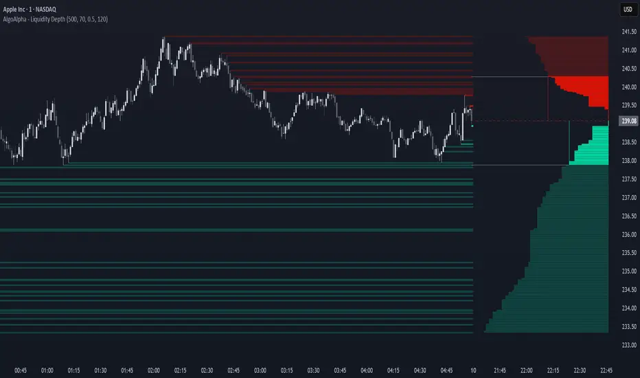
Liquidity Depth [AlgoAlpha]OVERVIEW
This script visualizes market liquidity by identifying key price levels where significant volume has transacted. It highlights zones of high buying and selling interest, helping traders understand where liquidity is accumulating and how price may respond to these areas. By dynamically tracking volume at highs and lows, the script builds a real-time liquidity profile, making it a powerful tool for identifying potential support and resistance levels.
CONCEPTS
Liquidity depth analysis helps traders determine how price interacts with supply and demand at different levels. The script processes historical volume data to distinguish between high-liquidity and low-liquidity zones. It assigns transparency levels to plotted lines , ensuring that more relevant liquidity areas stand out visually. The script adds a profile to show the depth of liquidity (derived from historical volume data) for levels above and below the current price
FEATURES
Liquidity Levels: Tracks liquidity levels based on volume concentration at price high and lows.
Volume-Based Transparency: More significant liquidity levels are displayed with higher visibility, showing their significance.
Interpolation: interpolates the bullish and bearish liquidity depth at a user defined range away from the price, helping in comparing the liquidity amounts between bullish and bearish.
Depth Profile: Allows traders to visualize depth of liquidity in a more quantitative and clearer way than the liquidity levels/list]
USAGE
This indicator is best used to track liquidity levels and potential price reaction areas. Traders can adjust the Liquidity Lookback setting to analyze past liquidity levels over different historical periods. The Profile Resolution setting controls the granularity of liquidity depth visualization, with higher values providing more detail. The script can be applied across different timeframes, from intraday scalping to swing trading analysis. The plotted liquidity zones provide traders with insights into where price may encounter strong support, resistance, or potential liquidity-driven reversals.
TrinityBar**TrinityBar Strategy Description**
The TrinityBar strategy is a price‐action based trading model that leverages Bill Williams’ bar thirds concept to generate entry signals and execute market orders automatically. Here’s how it works:
1. **Bar Thirds Calculation:**
The strategy calculates the range of both the current fully formed bar and the previous fully formed bar. It then divides each bar’s range into three equal parts (thirds).
- For the current bar, the lower third and upper third levels are computed.
- The same is done for the previous bar.
2. **Bar Type Classification:**
Each bar is classified into one of several types based on where its open and close fall relative to its thirds:
- **Bullish Patterns:**
- *1‑3 Bar:* Opens in the lower third and closes in the upper third.
- *2‑3 Bar:* Opens in the middle third and closes in the upper third.
- *3‑3 Bar:* Both open and close are in the upper third.
- **Bearish Patterns:**
- *3‑1 Bar:* Opens in the upper third and closes in the lower third.
- *2‑1 Bar:* Opens in the middle third and closes in the lower third.
- *1‑1 Bar:* Both open and close are in the lower third.
3. **Signal Generation:**
- **Bullish Signal:** A valid buy is generated when the previous bar exhibits any bullish pattern (1‑3, 2‑3, or 3‑3) and the current bar is either a 1‑3 or a 3‑3 bar.
- **Bearish Signal:** A valid sell is generated when the previous bar shows any bearish pattern (1‑1, 2‑1, or 3‑1) and the current bar is either a 1‑1 or a 3‑1 bar.
4. **Visual Alerts:**
When a valid signal is identified, the strategy plots a small triangle below the bar for a buy signal (labeled “B” in green) and a triangle above the bar for a sell signal (labeled “S” in red).
5. **Trade Execution:**
Once a signal is confirmed:
- If a bullish signal is generated, any short positions are closed, and if there is no existing long position, a market long order is entered.
- Conversely, if a bearish signal occurs, any long positions are closed, and a market short order is entered if not already in a short position.
This strategy is designed to capture significant price expansions by relying solely on price action and bar structure, without relying on lagging indicators. It provides a mechanical, systematic approach that removes emotional bias from trading decisions.