Gap Reversal Signal with Indicators🔍 Gap Reversal Signal with Indicators — 結合 KD、MACD、SAR 與背離分析的多功能指標
🔍 Gap Reversal Signal with Indicators — A Multi-Tool Signal Indicator Combining KD, MACD, SAR, and Divergence Analysis
中文說明:
本指標結合多種常用技術分析工具,包括 KD 隨機指標、MACD 動能交叉、SAR 趨勢方向、以及 MACD 背離偵測,用以辨識潛在的價格反轉區域。適用於日內交易與波段操作,支援各類市場,如加密貨幣、股票與外匯等。
English Description:
This indicator combines several popular technical tools: Stochastic KD, MACD momentum crossovers, SAR trend direction, and MACD divergence detection. It helps traders identify potential reversal areas and is ideal for both intraday and swing trading. Works well on crypto, stocks, and forex markets.
🧠 功能特點 | Key Features
✅ KD指標(慢速隨機指標)檢測超買超賣並提供%K與%D交叉訊號
✅ Stochastic KD (slow) to detect overbought/oversold zones and crossover signals
✅ MACD金叉/死叉與零軸突破捕捉趨勢轉變與動能反轉
✅ MACD Crossovers + Zero-Line Breaks to capture trend changes and momentum reversals
✅ SAR指標即時顯示多空方向
✅ Parabolic SAR for real-time trend direction indication
✅ MACD背離偵測協助辨識潛在反轉區域
✅ MACD Divergence Detection for identifying hidden trend reversals
✅ 圖形提示與標籤提示可視化呈現各類訊號
✅ Visual Alerts and Labels for easy and quick signal recognition
📈 支援市場 | Supported Markets
📊 台股 / 美股 / 外匯 / 加密貨幣
📊 Taiwan Stocks / US Stocks / Forex / Cryptocurrencies (e.g. BTC, ETH)
🔧 推薦用法 | Recommended Use
搭配缺口策略與支撐壓力位使用
Use with gap-trading strategies and support/resistance zones
用於盤整末期或趨勢反轉的提示
Helpful for end-of-consolidation signals or trend reversals
支援短線與波段交易風格
Suitable for scalping and swing trading styles
💡 把這個指標加入你的圖表,立即體驗多重技術分析所帶來的交易優勢!
💡 Add this indicator to your chart now and experience the power of multi-tool technical analysis!
Cerca negli script per "parabolic SAR"
00 Averaging Down Backtest Strategy by RPAlawyer v21FOR EDUCATIONAL PURPOSES ONLY! THE CODE IS NOT YET FULLY DEVELOPED, BUT IT CAN PROVIDE INTERESTING DATA AND INSIGHTS IN ITS CURRENT STATE.
This strategy is an 'averaging down' backtester strategy. The goal of averaging/doubling down is to buy more of an asset at a lower price to reduce your average entry price.
This backtester code proves why you shouldn't do averaging down, but the code can be developed (and will be developed) further, and there might be settings even in its current form that prove that averaging down can be done effectively.
Different averaging down strategies exist:
- Linear/Fixed Amount: buy $1000 every time price drops 5%
- Grid Trading: Placing orders at price levels, often with increasing size, like $1000 at -5%, $2000 at -10%
- Martingale: doubling the position size with each new entry
- Reverse Martingale: decreasing position size as price falls: $4000, then $2000, then $1000
- Percentage-Based: position size based on % of remaining capital, like 10% of available funds at each level
- Dynamic/Adaptive: larger entries during high volatility, smaller during low
- Logarithmic: position sizes increase logarithmically as price drops
Unlike the above average costing strategies, it applies averaging down (I use DCA as a synonym) at a very strong trend reversal. So not at a certain predetermined percentage negative PNL % but at a trend reversal signaled by an indicator - hence it most closely resembles a dynamically moving grid DCA strategy.
Both entering the trade and averaging down assume a strong trend. The signals for trend detection are provided by an indicator that I published under the name '00 Parabolic SAR Trend Following Signals by RPAlawyer', but any indicator that generates numeric signals of 1 and -1 for buy and sell signals can be used.
The indicator must be connected to the strategy: in the strategy settings under 'External Source' you need to select '00 Parabolic SAR Trend Following Signals by RPAlawyer: Connector'. From this point, the strategy detects when the indicator generates buy and sell signals.
The strategy considers a strong trend when a buy signal appears above a very conservative ATR band, or a sell signal below the ATR band. The conservative ATR is chosen to filter ranging markets. This very conservative ATR setting has a default multiplier of 8 and length of 40. The multiplier can be increased up to 10, but there will be very few buy and sell signals at that level and DCA requirements will be very high. Trade entry and DCA occur at these strong trends. In the settings, the 'ATR Filter' setting determines the entry condition (e.g., ATR Filter multiplier of 9), and the 'DCA ATR' determines when DCA will happen (e.g., DCA ATR multiplier of 6).
The DCA levels and DCA amounts are determined as follows:
The first DCA occurs below the DCA Base Deviation% level (see settings, default 3%) which acts as a threshold. The thick green line indicates the long position avg price, and the thin red line below the green line indicates the 3% DCA threshold for long positions. The thick red line indicates the short position avg price, and the thin red line above the thick red line indicates the short position 3% DCA threshold. DCA size multiplier defines the DCA amount invested.
If the loss exceeds 3% AND a buy signal arrives below the lower ATR band for longs, or a sell signal arrives above the upper ATR band for shorts, then the first DCA will be executed. So the first DCA won't happen at 3%, rather 3% is a threshold where the additional condition is that the price must close above or below the ATR band (let's say the first DCA occured at 8%) – this is why the code resembles a dynamic grid strategy, where the grid moves such that alongside the first 3% threshold, a strong trend must also appear for DCA. At this point, the thick green/red line moves because the avg price is modified as a result of the DCA, and the thin red line indicating the next DCA level also moves. The next DCA level is determined by the first DCA level, meaning modified avg price plus an additional +8% + (3% * the Step Scale Multiplier in the settings). This next DCA level will be indicated by the modified thin red line, and the price must break through this level and again break through the ATR band for the second DCA to occur.
Since all this wasn't complicated enough, and I was always obsessed by the idea that when we're sitting in an underwater position for days, doing DCA and waiting for the price to correct, we can actually enter a short position on the other side, on which we can realize profit (if the broker allows taking hedge positions, Binance allows this in Europe).
This opposite position in this strategy can open from the point AFTER THE FIRST DCA OF THE BASE POSITION OCCURS. This base position first DCA actually indicates that the price has already moved against us significantly so time to earn some money on the other side. Breaking through the ATR band is also a condition for entry here, so the hedge position entry is not automatic, and the condition for further DCA is breaking through the DCA Base Deviation (default 3%) and breaking through the ATR band. So for the 'hedge' or rather opposite position, the entry and further DCA conditions are the same as for the base position. The hedge position avg price is indicated by a thick black line and the Next Hedge DCA Level is indicated by a thin black line.
The TPs are indicated by green labels for base positions and red labels for hedge positions.
No SL built into the strategy at this point but you are free to do your coding.
Summary data can be found in the upper right corner.
The fantastic trend reversal indicator Machine learning: Lorentzian Classification by jdehorty can be used as an external indicator, choose 'backtest stream' for the external source. The ATR Band multiplicators need to be reduced to 5-6 when using Lorentz.
The code can be further developed in several aspects, and as I write this, I already have a few ideas 😊

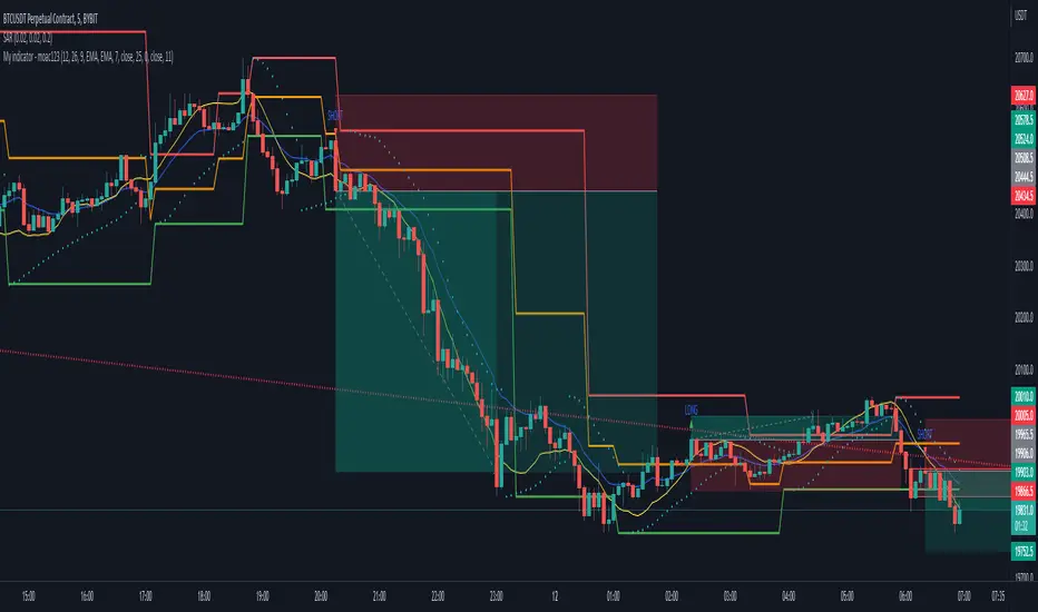
DIY Custom Strategy Builder [ZP] - v1DISCLAIMER:
This indicator as my first ever Tradingview indicator, has been developed for my personal trading analysis, consolidating various powerful indicators that I frequently use. A number of the embedded indicators within this tool are the creations of esteemed Pine Script developers from the TradingView community. In recognition of their contributions, the names of these developers will be prominently displayed alongside the respective indicator names. My selection of these indicators is rooted in my own experience and reflects those that have proven most effective for me. Please note that the past performance of any trading system or methodology is not necessarily indicative of future results. Always conduct your own research and due diligence before using any indicator or tool.
===========================================================================
Introducing the ultimate all-in-one DIY strategy builder indicator, With over 30+ famous indicators (some with custom configuration/settings) indicators included, you now have the power to mix and match to create your own custom strategy for shorter time or longer time frames depending on your trading style. Say goodbye to cluttered charts and manual/visual confirmation of multiple indicators and hello to endless possibilities with this indicator.
What it does
==================
This indicator basically help users to do 2 things:
1) Strategy Builder
With more than 30 indicators available, you can select any combination you prefer and the indicator will generate buy and sell signals accordingly. Alternative to the time-consuming process of manually confirming signals from multiple indicators! This indicator streamlines the process by automatically printing buy and sell signals based on your chosen combination of indicators. No more staring at the screen for hours on end, simply set up alerts and let the indicator do the work for you.
Available indicators that you can choose to build your strategy, are coded to seamlessly print the BUY and SELL signal upon confirmation of all selected indicators:
EMA Filter
2 EMA Cross
3 EMA Cross
Range Filter (Guikroth)
SuperTrend
Ichimoku Cloud
SuperIchi (LuxAlgo)
B-Xtrender (QuantTherapy)
Bull Bear Power Trend (Dreadblitz)
VWAP
BB Oscillator (Veryfid)
Trend Meter (Lij_MC)
Chandelier Exit (Everget)
CCI
Awesome Oscillator
DMI ( Adx )
Parabolic SAR
Waddah Attar Explosion (Shayankm)
Volatility Oscillator (Veryfid)
Damiani Volatility ( DV ) (RichardoSantos)
Stochastic
RSI
MACD
SSL Channel (ErwinBeckers)
Schaff Trend Cycle ( STC ) (LazyBear)
Chaikin Money Flow
Volume
Wolfpack Id (Darrellfischer1)
QQE Mod (Mihkhel00)
Hull Suite (Insilico)
Vortex Indicator
2) Overlay Indicators
Access the full potential of this indicator using the SWITCH BOARD section! Here, you have the ability to turn on and plot up to 14 of the included indicators on your chart. Simply select from the following options:
EMA
Support/Resistance (HeWhoMustNotBeNamed)
Supply/ Demand Zone ( SMC ) (Pmgjiv)
Parabolic SAR
Ichimoku Cloud
Superichi (LuxAlgo)
SuperTrend
Range Filter (Guikroth)
Average True Range (ATR)
VWAP
Schaff Trend Cycle ( STC ) (LazyBear)
PVSRA (TradersReality)
Liquidity Zone/Vector Candle Zone (TradersReality)
Market Sessions (Aurocks_AIF)
How it does it
==================
To explain how this indictor generate signal or does what it does, its best to put in points.
I have coded the strategy for each of the indicator, for some of the indicator you will see the option to choose strategy variation, these variants are either famous among the traders or its the ones I found more accurate based on my usage. By coding the strategy I will have the BUY and SELL signal generated by each indicator in the backend.
Next, the indicator will identify your selected LEADING INDICATOR and the CONFIRMATION INDICATOR(s).
On each candle close, the indicator will check if the selected LEADING INDICATOR generates signal (long or short).
Once the leading indicator generates the signal, then the indicator will scan each of the selected CONFIRMATION INDICATORS on candle close to check if any of the CONFIRMATION INDICATOR generated signal (long or short).
Until this point, all the process is happening in the backend, the indicator will print LONG or SHORT signal on the chart ONLY if LEADING INDICATOR and all the selected CONFIRMATION INDICATORS generates signal on candle close. example for long signal, the LEADING INDICATOR and all selected CONFIRMATION INDICATORS must print long signal.
The dashboard table will show your selected LEADING and CONFIRMATION INDICATORS and if LEADING or the CONFIRMATION INDICATORS have generated signal. Signal generated by LEADING and CONFIRMATION indicator whether long or short, is indicated by tick icon ✔. and if any of the selected CONFIRMATION or LEADING indicator does not generate signal on candle close, it will be indicated with cross symbol ✖.
how to use this indicator
==============================
Using the indicator is pretty simple, but it depends on your goal, whether you want to use it for overlaying the available indicators or using it to build your strategy or for both.
To use for Building your strategy: Select your LEADING INDICATOR, and then select your CONFIRMATION INDICATOR(s). if on candle close all the indicators generate signal, then this indicator will print SHORT or LONG signal on the chart for your entry. There are plenty of indicators you can use to build your strategy, some indicators are best for longer time frame setups while others are responsive indicators that are best for short time frame.
To use for overlaying the indicators: Open the setting of this indicator and scroll to the SWITCHBOARD section, from there you can select which indicator you want to plot on the chart.
For each of the listed indicators, you have the flexibility to customize the settings and configurations to suit your preferences. simply open indicator setting and scroll down, you will find configuration for each of the indicators used.
I will also release the Strategy Backtester for this indicator soon.

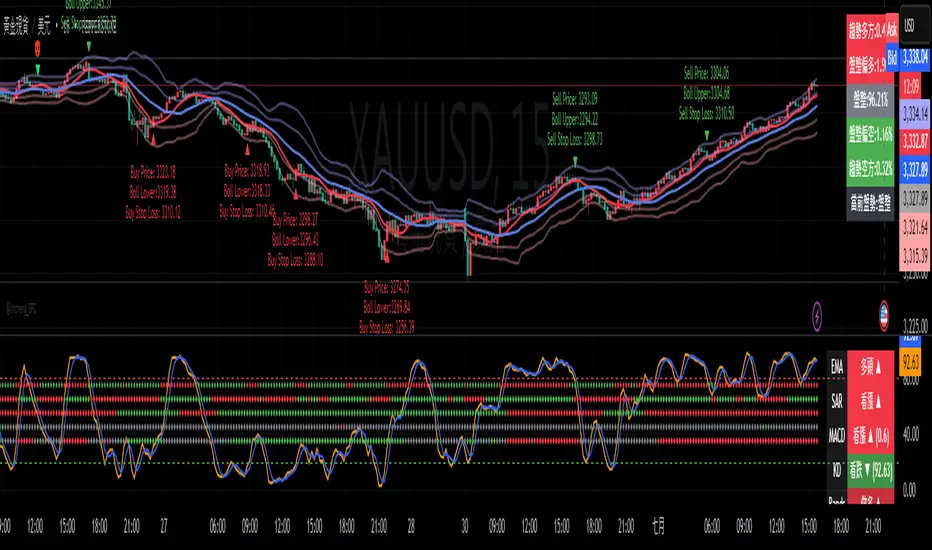
SumIndTarget:
The SumInd indicator combines Heiking Ashi, Sar Parabolic, Koncord, RSI, DMI, MACD and Bollinger Bands to give buy or sell signals or trends. This are called base indicators.
The goal is to have a clear and quick buy or sell suggestion and to avoid evaluating all or some of the named indicators, especially if they give contradictory signals among them. This speed and simplicity helps the trader to see several tickers in less time. It is intended for all markets and time periods where the above-mentioned indicators can be used.
How it works:
SumInd already has the importance or "weight" of each indicator named above configured, but they can be modified. You can set 0% for no use, or any other value based on the weight you want to give it, between 1% and 200% where 100% is the normal use, and increases or decreases based on importance.
Each base indicator can give signals to buy, sell or just "wait and see".
Each base indicator is checked for a buy signal, in which case its weight is added to the positive or green line, and if there is a sell signal, its weight is subtracted from the sell or red line. in case of indeterminacy or 'wait and see', nothing is added to any signal.
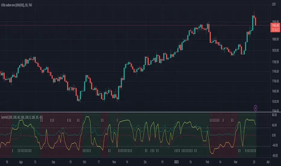
The yellow or total line is the sum of the buy or green signal plus the sell or red signal.
If the yellow or total line rises above the buy level, the background changes to green and an up arrow appears at the bottom of the chart indicating the buy suggestion, because most of the indicators you are interested in gave a buy signal.
If the yellow line or total falls below the sell level, the background changes to red and a downward arrow appears in the upper area of the chart indicating the sell suggestion, because most of the indicators you are interested in gave a sell signal.
The Buy and Sell level can be changed according to the security of the suggestion you need.
Areas without arrows or marks are considered "wait and see" areas, the previous trend in principle continues. They can be marked with the default background if desired from the SumInd settings.
Details and criterials:
Each of the following indicators can be turned on or off and assigned different weights of importances, by whether or not it shares the following criteria:
Heikin Ashi candles: add or subtract half an assigned weight if there is a buy or sell candle and the other half weight if there are two consecutive candles with the same signal.
RSI: Adds or subtracts the assigned weight if the ema is below or above the signal.
Parabolic Sar: Adds half a weight in transition to buy or sell and another half weight if there are two consecutive signals of the same trend.
Koncord: Add or subtract the weight if the current trend (mountain) grows or decreases respectively from the 4th previous time signal, and also the value (red line) is less than 35 or exceeds 65 respectively.
DMI: Adds or subtracts a quarter of the weight assigned by the DMI signal multiplied by the value of DMI, if the positive or negative signal exceeds the other negative or positive signal by 15% respectively.
Bollinger Bands: Add or subtract the weight if the previous third signal touches or falls out of the zone and keeps growing or decreasing respectively.
MACd: Add or subtract one third of the weight if the last 3 time signals are rising or falling, Add or subtract another third if the fast signal is above or below the slow signal, and Add or subtract the last third of the weight if it is rising with the negative fast signal, or falling with the positive fast signal.
Multi indicators tableThis is a comprehensive trading tool that presents an overview of the market in a tabular format. It consists of five distinct categories of trading indicators : Volatility, Trend, Momentum, Reversal, and Volume. Each category includes a series of indicators that are widely used in the trading communauty.
The Volatility category includes the Average True Range (ATR) and Bollinger Bands indicators. The Trend category comprises the Average Directional Index (ADX), four Exponential Moving Averages (EMAs), Aroon, Parabolic SAR, and the Supertrend. The Momentum category includes the Stochastic Relative Strength Index (StochRSI), Money Flow Index (MFI), Williams %R, Relative Strength Index (RSI), and Commodity Channel Index (CCI). The Reversal category includes Parabolic SAR, Moving Average Convergence Divergence (MACD), and PP Supertrend. Finally, the Volume category includes the Volume Exponential Moving Average (EMA) indicator.
The indicators states are easily readable, the indicator case is colored based on his actual state. A bullish color (green by default), a bearish color (red by default),
a very bullish color (dark green by default), a very bearish color (dark red by default) and a neutral color (gray by default) displayed when the indicator doesn't give us a clear signal. Some indicators do not have a very bullish or very bearish state. Concerning volatility indicators, the bullish color indicates high volatility, the bearish color indicates low volatility, and the neutral color indicates normal volatility.
Most of the indicators displayed in the table are customizable, and traders can choose to hide the categories they don't want to use. The Indicator provides a quick and easily readable view on the market and allows traders to reduce the number of indicators on their chart making it lighter and more readable.

[MT] Strategy Backtest Template| Initial Release | | EN |
An update of my old script, this script is designed so that it can be used as a template for all those traders who want to save time when programming their strategy and backtesting it, having functions already programmed that in normal development would take you more time to program, with this template you can simply add your favorite indicator and thus be able to take advantage of all the functions that this template has.
🔴Stop Loss and 🟢Take Profit:
No need to mention that it is a Stop Loss and a Take Profit, within these functions we find the options of: fixed percentage (%), fixed price ($), ATR, especially for Stop Loss we find the Pivot Points, in addition to this, the price range between the entry and the Stop Loss can be converted into a trailing stop loss, instead, especially for the Take Profit we have an option to choose a 1:X ratio that complements very well with the Pivot Points.
📈Heikin Ashi Based Entries:
Heikin Ashi entries are trades that are calculated based on Heikin Ashi candles but their price is executed to Japanese candles, thus avoiding false results that occur in Heikin candlestick charts, this making in certain cases better results in strategies that are executed with this option compared to Japanese candlesticks.
📊Dashboard:
A more visual and organized way to see the results and necessary data produced by our strategy, among them we can see the dates between which our operations are made regardless if you have activated some time filter, usual data such as Profit, Win Rate, Profit factor are also displayed in this panel, additionally data such as the total number of operations, how many were gains and how many losses, the average profit and loss for each operation and finally the maximum profits and losses followed, which are data that will be very useful to us when we elaborate our strategies.
Feel free to use this template to program your own strategies, if you find errors or want to request a new feature let me know in the comments or through my social networks found in my tradingview profile.
| Update 1.1 | | EN |
➕Additions: '
Time sessions filter and days of the week filter added to the time filter section.
Option to add leverage to the strategy.
5 Moving Averages, RSI, Stochastic RSI, ADX, and Parabolic Sar have been added as indicators for the strategy.
You can choose from the 6 available indicators the way to trade, entry alert or entry filter.
Added the option of ATR for Take Profit.
Ticker information and timeframe are now displayed on the dashboard.
Added display customization and color customization of indicator plots.
Added customization of display and color plots of trades displayed on chart.
📝Changes:
Now when activating the time filter it is optional to add a start or end date and time, being able to only add a start date or only an end date.
Operation plots have been changed from plot() to line creation with line.new().
Indicator plots can now be controlled from the "plots" section.
Acceptable and deniable range of profit, winrate and profit factor can now be chosen from the "plots" section to be displayed on the dashboard.
Aesthetic changes in the section separations within the settings section and within the code itself.
The function that made the indicators give inputs based on heikin ashi candles has been changed, see the code for more information.
⚙️Fixes:
Dashboard label now projects correctly on all timeframes including custom timeframes.
Removed unnecessary lines and variables to take up less code space.
All code in general has been optimized to avoid the use of variables, unnecessary lines and avoid unnecessary calculations, freeing up space to declare more variables and be able to use fewer lines of code.
| Lanzamiento Inicial | | ES |
Una actualización de mi antiguo script, este script está diseñado para que pueda ser usado como una plantilla para todos aquellos traders que quieran ahorrar tiempo al programar su estrategia y hacer un backtesting de ella, teniendo funciones ya programadas que en el desarrollo normal te tomaría más tiempo programar, con esta plantilla puedes simplemente agregar tu indicador favorito y así poder aprovechar todas las funciones que tiene esta plantilla.
🔴Stop Loss y 🟢Take Profit:
No hace falta mencionar que es un Stop Loss y un Take Profit, dentro de estas funciones encontramos las opciones de: porcentaje fijo (%), precio fijo ($), ATR, en especial para Stop Loss encontramos los Pivot Points, adicionalmente a esto, el rango de precio entre la entrada y el Stop Loss se puede convertir en un trailing stop loss, en cambio, especialmente para el Take Profit tenemos una opción para elegir un ratio 1:X que se complementa muy bien con los Pivot Points.
📈Entradas Basadas en Heikin Ashi:
Las entradas Heikin Ashi son operaciones que son calculados en base a las velas Heikin Ashi pero su precio esta ejecutado a velas japonesas, evitando así́ los falsos resultados que se producen en graficas de velas Heikin, esto haciendo que en ciertos casos se obtengan mejores resultados en las estrategias que son ejecutadas con esta opción en comparación con las velas japonesas.
📊Panel de Control:
Una manera más visual y organizada de ver los resultados y datos necesarios producidos por nuestra estrategia, entre ellos podemos ver las fechas entre las que se hacen nuestras operaciones independientemente si se tiene activado algún filtro de tiempo, datos usuales como el Profit, Win Rate, Profit factor también son mostrados en este panel, adicionalmente se agregaron datos como el número total de operaciones, cuantos fueron ganancias y cuantos perdidas, el promedio de ganancias y pérdidas por cada operación y por ultimo las máximas ganancias y pérdidas seguidas, que son datos que nos serán muy útiles al elaborar nuestras estrategias.
Siéntete libre de usar esta plantilla para programar tus propias estrategias, si encuentras errores o quieres solicitar una nueva función házmelo saber en los comentarios o a través de mis redes sociales que se encuentran en mi perfil de tradingview.
| Actualización 1.1 | | ES |
➕Añadidos:
Filtro de sesiones de tiempo y filtro de días de la semana agregados al apartado de filtro de tiempo.
Opción para agregar apalancamiento a la estrategia.
5 Moving Averages, RSI, Stochastic RSI, ADX, y Parabolic Sar se han agregado como indicadores para la estrategia.
Puedes escoger entre los 6 indicadores disponibles la forma de operar, alerta de entrada o filtro de entrada.
Añadido la opción de ATR para Take Profit.
La información del ticker y la temporalidad ahora se muestran en el dashboard.
Añadido personalización de visualización y color de los plots de indicadores.
Añadido personalización de visualización y color de los plots de operaciones mostradas en grafica.
📝Cambios:
Ahora al activar el filtro de tiempo es opcional añadir una fecha y hora de inicio o fin, pudiendo únicamente agregar una fecha de inicio o solamente una fecha de fin.
Los plots de operaciones han cambiados de plot() a creación de líneas con line.new().
Los plots de indicadores ahora se pueden controlar desde el apartado "plots".
Ahora se puede elegir el rango aceptable y negable de profit, winrate y profit factor desde el apartado "plots" para mostrarse en el dashboard.
Cambios estéticos en las separaciones de secciones dentro del apartado de configuraciones y dentro del propio código.
Se ha cambiado la función que hacía que los indicadores dieran entradas en base a velas heikin ashi, mire el código para más información.
⚙️Arreglos:
El dashboard label ahora se proyecta correctamente en todas las temporalidades incluyendo las temporalidades personalizadas.
Se han eliminado líneas y variables innecesarias para ocupar menos espacio en el código.
Se ha optimizado todo el código en general para evitar el uso de variables, líneas innecesarias y evitar los cálculos innecesarios, liberando espacio para declarar más variables y poder utilizar menos líneas de código.

MACD S/R signal indicatorI've based the script on my MACDs/r indicator.
I think it works better on higher timeframes, this is just an experiment, please feel free to modify it.
I have been testing it with parabolic SARS to know when to exit the trades.
Exit condition: if I'm in a log position and the price is below the last bearish parabolic SARS dot I exit the trade and the opposite for shorts
DISCLAIMER: Is just an experiment and I haven't test it with real money, be careful
Crypto High Potential StrategyBTCUSD -- 5 min
BUY POSITION
1 : The price is above the EMA
2 : The Parabolic SAR is green
3 : The RSI is above the 50 line
SELL POSITION
1 : The price is bellow the EMA
2 : The Parabolic SAR is red
3 : The rsi is below the 50 line

Nifty & BN 2 Candle Theory Back Testing and Alert Notification How To Initiate Long Trade-in Index Future/ Buy Call Options – 3 Min TF
▪ If The Index Futures Trades Above The VWAP, the Following Parameters are Checked For 2 Candle Theory on the long side
▪ RSI Trades Above 50 & Between 50-75/80
▪ Volume Of 2 Consecutive Bars Is Above 50 K for BN & 125 K For Nifty
▪ All the indicators (Parabolic SAR, Super Trend, VMA, VWAP) Below the Candles
▪ When the above conditions are met enter In 3rd Candle, With 1st Candle High As SL
How I Initiate Short Trade-In Index Future/ Buy Put Options – 3 Min TF
▪ If The Index Futures Trades Below The VWAP, the Following Parameters are Checked For 2 Candle Theory on the short side
▪ RSI Trades Below 40 & Between 40-25/20
▪ Volume Of 2 Consecutive Bars Is Above 50 K for BN & 125 K For Nifty
▪ All the Indicators (Parabolic SAR, Super Trend, VMA, VWAP) Above The Candles
▪ When the above conditions are met enter In 3rd Candle, With 1st Candle High As SL
The indicator checks the above and notifies to enter a long trade and short trade respectively. There is also volume cutoff and change in the volumes respectively, also non-trading times that can be set.

1 Indicator to rule them allThe best combination indicator consisting of 4 SMA's, 4 EMA's, Donchian Channels, Parabolic SAR, Bollinger Bands, Ichimoku Cloud, a trend strength highlight for the bollinger bands background according to the ADX, labels on the chart to draw in when the Directional Index plus and minus cross, and a background highlight for low and high volatility according to the Historical Volatility Percentile.
The Indicators and placed and group intentionally, with the SMA and EMA's next to the Donchian Channels to draw in areas of support and resistance, with the parabolic SAR afterwards for confirmation on entries and exits.
Next are the Bollinger Bands and the Ichimoku cloud, which when used in combination by an experienced trader allows one to see the trend and spot any developing opportunities at a glance. These can be used in combination with the ADX background in the bolls to point out when trends start and end.
The Directional Indexes crossing implies a equilibrium point has been reached between the buy and selling pressure. Finally the background highlight according to low and high periods of volatility does well to ensure you're entering into the best trades at the best times.
These indicators used together in combo with momentum oscillators will lead to a full and complete picture of the trend and the most likely places for future price to come, allowing a holistic view and confluence between different, noncollinear indicators to paint occam's razor onto the charts.
7 Moving Averages [Plus]Moving Averages are price based, lagging (or reactive) indicators that display the average price of a security over a set period of time. A Moving Average is a good way to gauge momentum as well as to confirm trends, and define areas of support and resistance. Essentially, Moving Averages smooth out the “noise” when trying to interpret charts. Noise is made up of fluctuations of both price and volume. Because a Moving Average is a lagging indicator and reacts to events that have already happened, it is not used as a predictive indicator but as an interpretive one for confirmations and analysis.
Bollinger Bands (BB) are a widely popular technical analysis instrument created by John Bollinger. The BB consist of a band of three lines which are plotted in relation to security prices. The line in the middle is usually a Simple Moving Average (SMA) set to a period of 20 days (the type of trend line and period can be changed by the trader; however a 20 day moving average is by far the most popular). The SMA then serves as a base for the Upper and Lower Bands which are used as a way to measure volatility by observing the relationship between the Bands and price. Typically the Upper and Lower Bands are set to two standard deviations away from the SMA (The Middle Line); however the number of standard deviations can also be adjusted by the trader.
This script shows 6 moving averages and Bollinger Bands.
Features:
- Standard MA inputs.
- MA type.
- MA period.
- MA source.
- MA resolution (time frame).
- MA Offset.
- Forecasting : forcasted prices are calculated using our MAType and MASource for the MAPeriod.
- Trail: Show only candles not included in the MA calculation.
The color of MA1 depends on the chosen strategy, by default this is the 3EMA strategy. You can also select "Pivot Point Supertrend" or "Ichimoku Trend"
Added "Parabolic Stop and Reverse (PSAR)" . The PSAR is a time and price technical analysis tool primarily used to identify points of potential stops and reverses. In fact, the SAR in Parabolic SAR stands for "Stop and Reverse". The indicator's calculations create a parabola which is located below price during a Bullish Trend and above Price during a Bearish Trend.
Added "Linear Regression Channel" which can be correctly plotted on logarithmic charts. A linear regression channel consists of a median line with 2 parallel lines, above and below it, at the same distance. Those lines can be seen as support and resistance. The median line is calculated based on linear regression of the closing prices but the source can also be set to open, high or low. The height of the channel is based on the deviation of price to the median line. Extrapolating the channel forward can help to provide a bias and to find trading opportunities.
[VJ]Phoenix Force of PSAR +MACD +RSIThis is a simple intraday strategy for working on Stocks or commodities based out on PSAR, MACD , RSI and chop index . You can modify the start time and end time based on your timezones. Session value should be from market start to the time you want to square-off
Important: The end time should be at least 2 minutes before the intraday square-off time set by your broker
Comment below if you get good returns
Strategy: Entry Exits using PSAR and momentum and trend using MACD and RSI. A chop index is used as filtering
Indicators used :
Parabolic SAR is a technical indicator that is used to determine the price direction of stocks and it also draws attention to the traders when the price is changing
PSAR helps you:
Identify when a certain price trend is going to change direction
Indicate the most effective level at which to enter into the trade
Indicate the most effective exit point for the trade
Moving average convergence divergence (MACD) is a trend-following momentum indicator that shows the relationship between two moving averages of a security's price. ... Traders may buy the security when the MACD crosses above its signal line and sell—or short—the security when the MACD crosses below the signal line
RSI is intended to chart the current and historical strength or weakness of a stock or market based on the closing prices of a recent trading period.
Buying/Selling
When trading with the parabolic SAR, you would buy a market when the dots move below the current asset price and are green in colour. Alternatively, you would sell a market when the dots move above the current asset price and are red in colour. We use MACD , RSI to ensure that a right trade is picked when PSAR gives an indication. CI is used to stay away from the range bound market as much as possible.
Usage & Best setting :
Choose a good volatile stock and a time frame - 5m.
MA length : 200
RSI threshold : 50
MACD: 12,26,9
There is stop loss and take profit that can be used to optimise your trade
The template also includes daily square off based on your time.

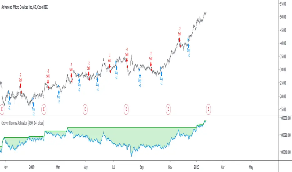
Grover Llorens Activator Strategy AnalysisThe Grover Llorens Activator is a trailing stop indicator deeply inspired by the parabolic SAR indicator, and aim to provide early exit points and reversal detection. The indicator was posted not so long ago, you can find it here :
Today a strategy using the indicator is proposed, and its profitability is analyzed on 3 different markets with the main time frame being 1 hour, remember that lower time frames involve lower absolute price changes, therefore we are way more affected by the spread, and we can require a larger position sizing depending on our investment target, trading higher time-frames is always a good practice and this is why 1 hour is selected. Based on the result we might make various conclusions regarding the indicator accuracy and might have ideas on future improvements of the indicator.
I'am not great when it comes to strategy design, i still hope to share correct and useful information in this post, let me know your thoughts on the post format and if i should make more of these.
Setup And Rules
The analysis is solely based on the indicator signals, money management isn't taken into account, this allow us to have an idea on the indicator robustness and resilience, particularly on extremely volatile markets and ones exhibiting a chaotic structure, altho it is normally good practice to close any position before a market closure in order to avoid any potential major gaps.
The settings used are 480 for length and 14 for mult, this create relatively mid term signals that are suited for a trend indicator such as the Grover Llorens Activator, unfortunately we can't infer the indicator optimal settings, thats how it is with any technical indicator anyway.
Here are the rules of our strategy :
long : closing price cross over the indicator
short : closing price cross under the indicator
We use constant position sizing, once a signal is triggered all the previous positions are closed.
Description Of The Statistics Used
Various statistics are presented in this post, here is a brief description of the main ones :
Percent Profitability (higher = better): Percentage of winning trades, that is : winning trades/total number of trades × 100
Maximum Drawdown (lower = better) : The highest difference between a peak and a valley in the balance, that is : peak - valley , in percentage : (peak - valley)/peak × 100
Profit Factor (higher = better) : Gross profit divided by gross loss, values under 1 represent gross losses superior to the gross profits
Remember that more volatility = more risk, since higher absolute price changes can logically cause larger losses.
EURUSD
The first market analyzed is the Forex market with the EURUSD major pair with a position sizing of 1000 units (1 micro lot). Since October EURUSD is not showing any particular strong trend but posses a discrete rising motion, fortunately cycles can be observed.
The equity was rising until two trades appeared causing a decline in the equity. Before October a bearish market could be observed.
We can see that the equity is rising, the trend still posses various retracements that affect our indicator, however we can see that the indicator totally nail the end of the trend, thats the power of converging toward the price.
In short :
$ 86.63 net profit
340 closed trades
37.65 % profitable (thats a lot of loosing trades)
1.19 profit factor
$ 76.67 max drawdown
Applying a spread would create negative results (in general the average spread is used), not a great start...
BTCUSD
The cryptocurrency market is relatively more volatile than others, which also mean potentially higher returns, we test the indicator using certainly the most traded cryptocurrency, BTCUSD. We will use a position sizing of 1 unit.
In the case of BTCUSD the strategy balance is relatively stationary around the initial capital, with of course high dispersion.
from september to december the market is bearish with various ranging periods, no apparent cycles can be observed, except maybe in the ranging period of october, this ranging period is followed by a non linear trend (relatively parabolic) that the indicator failed to capture in its integrity (this is a recurrent problem and it is starting to piss me off xD).
In short :
$ 2010.64 net profit (aka how i bet the crypto market)
395 closed trades
38.23 % profitable
1.036 profit factor
$ 5738.01 max drawdown (aka how i lost to the crypto market)
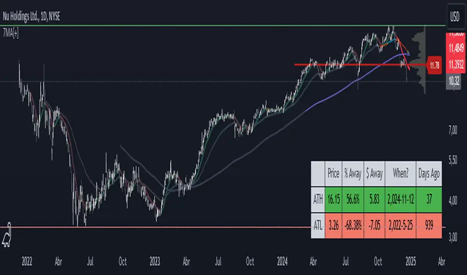
AMD
AMD stand for Advanced Micro Devices and is a company focused on the development of computer technology, i love the microprocessor market and i really like AMD who start this year in a pretty great way with a net bullish trend.
The performance of the indicator on AMD is decent (at last !) with the equity producing many new higher highs. The indicator performance still drop in the middle end of 2019 with a large equity drawdown of 17$ caused by the gap of august 8. Unfortunately AMD, like lot of well behaving stocks can only tells us that the indicator has good performances on heavily trending markets with no excess of noise or chaotic structures.
In short :
$ 17.86 net profit (Enough for a consistent lunch)
295 closed trades
36.27 % profitable
1.414 profit factor
$ 10.37 max drawdown.
Conclusion
A strategy using the recently proposed Grover Llorens activator has been presented. We can easily conclude that the indicator can't possibly generate long term returns under chaotic and volatile markets, and could even produce unnecessary trades in trending markets without much parasitic fluctuations such as noise and retracements (think about a simple linear trend) since the indicator converge toward the price and would therefore automatically cross over/under the trend, thus guaranteeing a false signal.
However we have seen its ability to provide accurate early reversal detection shine from time to time, thus over performing lagging indicators in this aspect, however the duration of price fluctuations isn't fixed at a certain period, the rate of convergence should be way faster during volatile fluctuations, of moderate speed during more cyclic fluctuations, and really slow with apparent long term trends, this could be achieved by making the indicator adaptive, but it won't really make it necessarily perform better.
That said i still believe that converging trend indicators are really interesting and aim to capture the non lasting behavior of price fluctuations, they shouldn't receive so much hate (think about the poor p-sar).
Thanks for reading !
Markov Chain [3D] | FractalystWhat exactly is a Markov Chain?
This indicator uses a Markov Chain model to analyze, quantify, and visualize the transitions between market regimes (Bull, Bear, Neutral) on your chart. It dynamically detects these regimes in real-time, calculates transition probabilities, and displays them as animated 3D spheres and arrows, giving traders intuitive insight into current and future market conditions.
How does a Markov Chain work, and how should I read this spheres-and-arrows diagram?
Think of three weather modes: Sunny, Rainy, Cloudy.
Each sphere is one mode. The loop on a sphere means “stay the same next step” (e.g., Sunny again tomorrow).
The arrows leaving a sphere show where things usually go next if they change (e.g., Sunny moving to Cloudy).
Some paths matter more than others. A more prominent loop means the current mode tends to persist. A more prominent outgoing arrow means a change to that destination is the usual next step.
Direction isn’t symmetric: moving Sunny→Cloudy can behave differently than Cloudy→Sunny.
Now relabel the spheres to markets: Bull, Bear, Neutral.
Spheres: market regimes (uptrend, downtrend, range).
Self‑loop: tendency for the current regime to continue on the next bar.
Arrows: the most common next regime if a switch happens.
How to read: Start at the sphere that matches current bar state. If the loop stands out, expect continuation. If one outgoing path stands out, that switch is the typical next step. Opposite directions can differ (Bear→Neutral doesn’t have to match Neutral→Bear).
What states and transitions are shown?
The three market states visualized are:
Bullish (Bull): Upward or strong-market regime.
Bearish (Bear): Downward or weak-market regime.
Neutral: Sideways or range-bound regime.
Bidirectional animated arrows and probability labels show how likely the market is to move from one regime to another (e.g., Bull → Bear or Neutral → Bull).
How does the regime detection system work?
You can use either built-in price returns (based on adaptive Z-score normalization) or supply three custom indicators (such as volume, oscillators, etc.).
Values are statistically normalized (Z-scored) over a configurable lookback period.
The normalized outputs are classified into Bull, Bear, or Neutral zones.
If using three indicators, their regime signals are averaged and smoothed for robustness.
How are transition probabilities calculated?
On every confirmed bar, the algorithm tracks the sequence of detected market states, then builds a rolling window of transitions.
The code maintains a transition count matrix for all regime pairs (e.g., Bull → Bear).
Transition probabilities are extracted for each possible state change using Laplace smoothing for numerical stability, and frequently updated in real-time.
What is unique about the visualization?
3D animated spheres represent each regime and change visually when active.
Animated, bidirectional arrows reveal transition probabilities and allow you to see both dominant and less likely regime flows.
Particles (moving dots) animate along the arrows, enhancing the perception of regime flow direction and speed.
All elements dynamically update with each new price bar, providing a live market map in an intuitive, engaging format.
Can I use custom indicators for regime classification?
Yes! Enable the "Custom Indicators" switch and select any three chart series as inputs. These will be normalized and combined (each with equal weight), broadening the regime classification beyond just price-based movement.
What does the “Lookback Period” control?
Lookback Period (default: 100) sets how much historical data builds the probability matrix. Shorter periods adapt faster to regime changes but may be noisier. Longer periods are more stable but slower to adapt.
How is this different from a Hidden Markov Model (HMM)?
It sets the window for both regime detection and probability calculations. Lower values make the system more reactive, but potentially noisier. Higher values smooth estimates and make the system more robust.
How is this Markov Chain different from a Hidden Markov Model (HMM)?
Markov Chain (as here): All market regimes (Bull, Bear, Neutral) are directly observable on the chart. The transition matrix is built from actual detected regimes, keeping the model simple and interpretable.
Hidden Markov Model: The actual regimes are unobservable ("hidden") and must be inferred from market output or indicator "emissions" using statistical learning algorithms. HMMs are more complex, can capture more subtle structure, but are harder to visualize and require additional machine learning steps for training.
A standard Markov Chain models transitions between observable states using a simple transition matrix, while a Hidden Markov Model assumes the true states are hidden (latent) and must be inferred from observable “emissions” like price or volume data. In practical terms, a Markov Chain is transparent and easier to implement and interpret; an HMM is more expressive but requires statistical inference to estimate hidden states from data.
Markov Chain: states are observable; you directly count or estimate transition probabilities between visible states. This makes it simpler, faster, and easier to validate and tune.
HMM: states are hidden; you only observe emissions generated by those latent states. Learning involves machine learning/statistical algorithms (commonly Baum–Welch/EM for training and Viterbi for decoding) to infer both the transition dynamics and the most likely hidden state sequence from data.
How does the indicator avoid “repainting” or look-ahead bias?
All regime changes and matrix updates happen only on confirmed (closed) bars, so no future data is leaked, ensuring reliable real-time operation.
Are there practical tuning tips?
Tune the Lookback Period for your asset/timeframe: shorter for fast markets, longer for stability.
Use custom indicators if your asset has unique regime drivers.
Watch for rapid changes in transition probabilities as early warning of a possible regime shift.
Who is this indicator for?
Quants and quantitative researchers exploring probabilistic market modeling, especially those interested in regime-switching dynamics and Markov models.
Programmers and system developers who need a probabilistic regime filter for systematic and algorithmic backtesting:
The Markov Chain indicator is ideally suited for programmatic integration via its bias output (1 = Bull, 0 = Neutral, -1 = Bear).
Although the visualization is engaging, the core output is designed for automated, rules-based workflows—not for discretionary/manual trading decisions.
Developers can connect the indicator’s output directly to their Pine Script logic (using input.source()), allowing rapid and robust backtesting of regime-based strategies.
It acts as a plug-and-play regime filter: simply plug the bias output into your entry/exit logic, and you have a scientifically robust, probabilistically-derived signal for filtering, timing, position sizing, or risk regimes.
The MC's output is intentionally "trinary" (1/0/-1), focusing on clear regime states for unambiguous decision-making in code. If you require nuanced, multi-probability or soft-label state vectors, consider expanding the indicator or stacking it with a probability-weighted logic layer in your scripting.
Because it avoids subjectivity, this approach is optimal for systematic quants, algo developers building backtested, repeatable strategies based on probabilistic regime analysis.
What's the mathematical foundation behind this?
The mathematical foundation behind this Markov Chain indicator—and probabilistic regime detection in finance—draws from two principal models: the (standard) Markov Chain and the Hidden Markov Model (HMM).
How to use this indicator programmatically?
The Markov Chain indicator automatically exports a bias value (+1 for Bullish, -1 for Bearish, 0 for Neutral) as a plot visible in the Data Window. This allows you to integrate its regime signal into your own scripts and strategies for backtesting, automation, or live trading.
Step-by-Step Integration with Pine Script (input.source)
Add the Markov Chain indicator to your chart.
This must be done first, since your custom script will "pull" the bias signal from the indicator's plot.
In your strategy, create an input using input.source()
Example:
//@version=5
strategy("MC Bias Strategy Example")
mcBias = input.source(close, "MC Bias Source")
After saving, go to your script’s settings. For the “MC Bias Source” input, select the plot/output of the Markov Chain indicator (typically its bias plot).
Use the bias in your trading logic
Example (long only on Bull, flat otherwise):
if mcBias == 1
strategy.entry("Long", strategy.long)
else
strategy.close("Long")
For more advanced workflows, combine mcBias with additional filters or trailing stops.
How does this work behind-the-scenes?
TradingView’s input.source() lets you use any plot from another indicator as a real-time, “live” data feed in your own script (source).
The selected bias signal is available to your Pine code as a variable, enabling logical decisions based on regime (trend-following, mean-reversion, etc.).
This enables powerful strategy modularity : decouple regime detection from entry/exit logic, allowing fast experimentation without rewriting core signal code.
Integrating 45+ Indicators with Your Markov Chain — How & Why
The Enhanced Custom Indicators Export script exports a massive suite of over 45 technical indicators—ranging from classic momentum (RSI, MACD, Stochastic, etc.) to trend, volume, volatility, and oscillator tools—all pre-calculated, centered/scaled, and available as plots.
// Enhanced Custom Indicators Export - 45 Technical Indicators
// Comprehensive technical analysis suite for advanced market regime detection
//@version=6
indicator('Enhanced Custom Indicators Export | Fractalyst', shorttitle='Enhanced CI Export', overlay=false, scale=scale.right, max_labels_count=500, max_lines_count=500)
// |----- Input Parameters -----| //
momentum_group = "Momentum Indicators"
trend_group = "Trend Indicators"
volume_group = "Volume Indicators"
volatility_group = "Volatility Indicators"
oscillator_group = "Oscillator Indicators"
display_group = "Display Settings"
// Common lengths
length_14 = input.int(14, "Standard Length (14)", minval=1, maxval=100, group=momentum_group)
length_20 = input.int(20, "Medium Length (20)", minval=1, maxval=200, group=trend_group)
length_50 = input.int(50, "Long Length (50)", minval=1, maxval=200, group=trend_group)
// Display options
show_table = input.bool(true, "Show Values Table", group=display_group)
table_size = input.string("Small", "Table Size", options= , group=display_group)
// |----- MOMENTUM INDICATORS (15 indicators) -----| //
// 1. RSI (Relative Strength Index)
rsi_14 = ta.rsi(close, length_14)
rsi_centered = rsi_14 - 50
// 2. Stochastic Oscillator
stoch_k = ta.stoch(close, high, low, length_14)
stoch_d = ta.sma(stoch_k, 3)
stoch_centered = stoch_k - 50
// 3. Williams %R
williams_r = ta.stoch(close, high, low, length_14) - 100
// 4. MACD (Moving Average Convergence Divergence)
= ta.macd(close, 12, 26, 9)
// 5. Momentum (Rate of Change)
momentum = ta.mom(close, length_14)
momentum_pct = (momentum / close ) * 100
// 6. Rate of Change (ROC)
roc = ta.roc(close, length_14)
// 7. Commodity Channel Index (CCI)
cci = ta.cci(close, length_20)
// 8. Money Flow Index (MFI)
mfi = ta.mfi(close, length_14)
mfi_centered = mfi - 50
// 9. Awesome Oscillator (AO)
ao = ta.sma(hl2, 5) - ta.sma(hl2, 34)
// 10. Accelerator Oscillator (AC)
ac = ao - ta.sma(ao, 5)
// 11. Chande Momentum Oscillator (CMO)
cmo = ta.cmo(close, length_14)
// 12. Detrended Price Oscillator (DPO)
dpo = close - ta.sma(close, length_20)
// 13. Price Oscillator (PPO)
ppo = ta.sma(close, 12) - ta.sma(close, 26)
ppo_pct = (ppo / ta.sma(close, 26)) * 100
// 14. TRIX
trix_ema1 = ta.ema(close, length_14)
trix_ema2 = ta.ema(trix_ema1, length_14)
trix_ema3 = ta.ema(trix_ema2, length_14)
trix = ta.roc(trix_ema3, 1) * 10000
// 15. Klinger Oscillator
klinger = ta.ema(volume * (high + low + close) / 3, 34) - ta.ema(volume * (high + low + close) / 3, 55)
// 16. Fisher Transform
fisher_hl2 = 0.5 * (hl2 - ta.lowest(hl2, 10)) / (ta.highest(hl2, 10) - ta.lowest(hl2, 10)) - 0.25
fisher = 0.5 * math.log((1 + fisher_hl2) / (1 - fisher_hl2))
// 17. Stochastic RSI
stoch_rsi = ta.stoch(rsi_14, rsi_14, rsi_14, length_14)
stoch_rsi_centered = stoch_rsi - 50
// 18. Relative Vigor Index (RVI)
rvi_num = ta.swma(close - open)
rvi_den = ta.swma(high - low)
rvi = rvi_den != 0 ? rvi_num / rvi_den : 0
// 19. Balance of Power (BOP)
bop = (close - open) / (high - low)
// |----- TREND INDICATORS (10 indicators) -----| //
// 20. Simple Moving Average Momentum
sma_20 = ta.sma(close, length_20)
sma_momentum = ((close - sma_20) / sma_20) * 100
// 21. Exponential Moving Average Momentum
ema_20 = ta.ema(close, length_20)
ema_momentum = ((close - ema_20) / ema_20) * 100
// 22. Parabolic SAR
sar = ta.sar(0.02, 0.02, 0.2)
sar_trend = close > sar ? 1 : -1
// 23. Linear Regression Slope
lr_slope = ta.linreg(close, length_20, 0) - ta.linreg(close, length_20, 1)
// 24. Moving Average Convergence (MAC)
mac = ta.sma(close, 10) - ta.sma(close, 30)
// 25. Trend Intensity Index (TII)
tii_sum = 0.0
for i = 1 to length_20
tii_sum += close > close ? 1 : 0
tii = (tii_sum / length_20) * 100
// 26. Ichimoku Cloud Components
ichimoku_tenkan = (ta.highest(high, 9) + ta.lowest(low, 9)) / 2
ichimoku_kijun = (ta.highest(high, 26) + ta.lowest(low, 26)) / 2
ichimoku_signal = ichimoku_tenkan > ichimoku_kijun ? 1 : -1
// 27. MESA Adaptive Moving Average (MAMA)
mama_alpha = 2.0 / (length_20 + 1)
mama = ta.ema(close, length_20)
mama_momentum = ((close - mama) / mama) * 100
// 28. Zero Lag Exponential Moving Average (ZLEMA)
zlema_lag = math.round((length_20 - 1) / 2)
zlema_data = close + (close - close )
zlema = ta.ema(zlema_data, length_20)
zlema_momentum = ((close - zlema) / zlema) * 100
// |----- VOLUME INDICATORS (6 indicators) -----| //
// 29. On-Balance Volume (OBV)
obv = ta.obv
// 30. Volume Rate of Change (VROC)
vroc = ta.roc(volume, length_14)
// 31. Price Volume Trend (PVT)
pvt = ta.pvt
// 32. Negative Volume Index (NVI)
nvi = 0.0
nvi := volume < volume ? nvi + ((close - close ) / close ) * nvi : nvi
// 33. Positive Volume Index (PVI)
pvi = 0.0
pvi := volume > volume ? pvi + ((close - close ) / close ) * pvi : pvi
// 34. Volume Oscillator
vol_osc = ta.sma(volume, 5) - ta.sma(volume, 10)
// 35. Ease of Movement (EOM)
eom_distance = high - low
eom_box_height = volume / 1000000
eom = eom_box_height != 0 ? eom_distance / eom_box_height : 0
eom_sma = ta.sma(eom, length_14)
// 36. Force Index
force_index = volume * (close - close )
force_index_sma = ta.sma(force_index, length_14)
// |----- VOLATILITY INDICATORS (10 indicators) -----| //
// 37. Average True Range (ATR)
atr = ta.atr(length_14)
atr_pct = (atr / close) * 100
// 38. Bollinger Bands Position
bb_basis = ta.sma(close, length_20)
bb_dev = 2.0 * ta.stdev(close, length_20)
bb_upper = bb_basis + bb_dev
bb_lower = bb_basis - bb_dev
bb_position = bb_dev != 0 ? (close - bb_basis) / bb_dev : 0
bb_width = bb_dev != 0 ? (bb_upper - bb_lower) / bb_basis * 100 : 0
// 39. Keltner Channels Position
kc_basis = ta.ema(close, length_20)
kc_range = ta.ema(ta.tr, length_20)
kc_upper = kc_basis + (2.0 * kc_range)
kc_lower = kc_basis - (2.0 * kc_range)
kc_position = kc_range != 0 ? (close - kc_basis) / kc_range : 0
// 40. Donchian Channels Position
dc_upper = ta.highest(high, length_20)
dc_lower = ta.lowest(low, length_20)
dc_basis = (dc_upper + dc_lower) / 2
dc_position = (dc_upper - dc_lower) != 0 ? (close - dc_basis) / (dc_upper - dc_lower) : 0
// 41. Standard Deviation
std_dev = ta.stdev(close, length_20)
std_dev_pct = (std_dev / close) * 100
// 42. Relative Volatility Index (RVI)
rvi_up = ta.stdev(close > close ? close : 0, length_14)
rvi_down = ta.stdev(close < close ? close : 0, length_14)
rvi_total = rvi_up + rvi_down
rvi_volatility = rvi_total != 0 ? (rvi_up / rvi_total) * 100 : 50
// 43. Historical Volatility
hv_returns = math.log(close / close )
hv = ta.stdev(hv_returns, length_20) * math.sqrt(252) * 100
// 44. Garman-Klass Volatility
gk_vol = math.log(high/low) * math.log(high/low) - (2*math.log(2)-1) * math.log(close/open) * math.log(close/open)
gk_volatility = math.sqrt(ta.sma(gk_vol, length_20)) * 100
// 45. Parkinson Volatility
park_vol = math.log(high/low) * math.log(high/low)
parkinson = math.sqrt(ta.sma(park_vol, length_20) / (4 * math.log(2))) * 100
// 46. Rogers-Satchell Volatility
rs_vol = math.log(high/close) * math.log(high/open) + math.log(low/close) * math.log(low/open)
rogers_satchell = math.sqrt(ta.sma(rs_vol, length_20)) * 100
// |----- OSCILLATOR INDICATORS (5 indicators) -----| //
// 47. Elder Ray Index
elder_bull = high - ta.ema(close, 13)
elder_bear = low - ta.ema(close, 13)
elder_power = elder_bull + elder_bear
// 48. Schaff Trend Cycle (STC)
stc_macd = ta.ema(close, 23) - ta.ema(close, 50)
stc_k = ta.stoch(stc_macd, stc_macd, stc_macd, 10)
stc_d = ta.ema(stc_k, 3)
stc = ta.stoch(stc_d, stc_d, stc_d, 10)
// 49. Coppock Curve
coppock_roc1 = ta.roc(close, 14)
coppock_roc2 = ta.roc(close, 11)
coppock = ta.wma(coppock_roc1 + coppock_roc2, 10)
// 50. Know Sure Thing (KST)
kst_roc1 = ta.roc(close, 10)
kst_roc2 = ta.roc(close, 15)
kst_roc3 = ta.roc(close, 20)
kst_roc4 = ta.roc(close, 30)
kst = ta.sma(kst_roc1, 10) + 2*ta.sma(kst_roc2, 10) + 3*ta.sma(kst_roc3, 10) + 4*ta.sma(kst_roc4, 15)
// 51. Percentage Price Oscillator (PPO)
ppo_line = ((ta.ema(close, 12) - ta.ema(close, 26)) / ta.ema(close, 26)) * 100
ppo_signal = ta.ema(ppo_line, 9)
ppo_histogram = ppo_line - ppo_signal
// |----- PLOT MAIN INDICATORS -----| //
// Plot key momentum indicators
plot(rsi_centered, title="01_RSI_Centered", color=color.purple, linewidth=1)
plot(stoch_centered, title="02_Stoch_Centered", color=color.blue, linewidth=1)
plot(williams_r, title="03_Williams_R", color=color.red, linewidth=1)
plot(macd_histogram, title="04_MACD_Histogram", color=color.orange, linewidth=1)
plot(cci, title="05_CCI", color=color.green, linewidth=1)
// Plot trend indicators
plot(sma_momentum, title="06_SMA_Momentum", color=color.navy, linewidth=1)
plot(ema_momentum, title="07_EMA_Momentum", color=color.maroon, linewidth=1)
plot(sar_trend, title="08_SAR_Trend", color=color.teal, linewidth=1)
plot(lr_slope, title="09_LR_Slope", color=color.lime, linewidth=1)
plot(mac, title="10_MAC", color=color.fuchsia, linewidth=1)
// Plot volatility indicators
plot(atr_pct, title="11_ATR_Pct", color=color.yellow, linewidth=1)
plot(bb_position, title="12_BB_Position", color=color.aqua, linewidth=1)
plot(kc_position, title="13_KC_Position", color=color.olive, linewidth=1)
plot(std_dev_pct, title="14_StdDev_Pct", color=color.silver, linewidth=1)
plot(bb_width, title="15_BB_Width", color=color.gray, linewidth=1)
// Plot volume indicators
plot(vroc, title="16_VROC", color=color.blue, linewidth=1)
plot(eom_sma, title="17_EOM", color=color.red, linewidth=1)
plot(vol_osc, title="18_Vol_Osc", color=color.green, linewidth=1)
plot(force_index_sma, title="19_Force_Index", color=color.orange, linewidth=1)
plot(obv, title="20_OBV", color=color.purple, linewidth=1)
// Plot additional oscillators
plot(ao, title="21_Awesome_Osc", color=color.navy, linewidth=1)
plot(cmo, title="22_CMO", color=color.maroon, linewidth=1)
plot(dpo, title="23_DPO", color=color.teal, linewidth=1)
plot(trix, title="24_TRIX", color=color.lime, linewidth=1)
plot(fisher, title="25_Fisher", color=color.fuchsia, linewidth=1)
// Plot more momentum indicators
plot(mfi_centered, title="26_MFI_Centered", color=color.yellow, linewidth=1)
plot(ac, title="27_AC", color=color.aqua, linewidth=1)
plot(ppo_pct, title="28_PPO_Pct", color=color.olive, linewidth=1)
plot(stoch_rsi_centered, title="29_StochRSI_Centered", color=color.silver, linewidth=1)
plot(klinger, title="30_Klinger", color=color.gray, linewidth=1)
// Plot trend continuation
plot(tii, title="31_TII", color=color.blue, linewidth=1)
plot(ichimoku_signal, title="32_Ichimoku_Signal", color=color.red, linewidth=1)
plot(mama_momentum, title="33_MAMA_Momentum", color=color.green, linewidth=1)
plot(zlema_momentum, title="34_ZLEMA_Momentum", color=color.orange, linewidth=1)
plot(bop, title="35_BOP", color=color.purple, linewidth=1)
// Plot volume continuation
plot(nvi, title="36_NVI", color=color.navy, linewidth=1)
plot(pvi, title="37_PVI", color=color.maroon, linewidth=1)
plot(momentum_pct, title="38_Momentum_Pct", color=color.teal, linewidth=1)
plot(roc, title="39_ROC", color=color.lime, linewidth=1)
plot(rvi, title="40_RVI", color=color.fuchsia, linewidth=1)
// Plot volatility continuation
plot(dc_position, title="41_DC_Position", color=color.yellow, linewidth=1)
plot(rvi_volatility, title="42_RVI_Volatility", color=color.aqua, linewidth=1)
plot(hv, title="43_Historical_Vol", color=color.olive, linewidth=1)
plot(gk_volatility, title="44_GK_Volatility", color=color.silver, linewidth=1)
plot(parkinson, title="45_Parkinson_Vol", color=color.gray, linewidth=1)
// Plot final oscillators
plot(rogers_satchell, title="46_RS_Volatility", color=color.blue, linewidth=1)
plot(elder_power, title="47_Elder_Power", color=color.red, linewidth=1)
plot(stc, title="48_STC", color=color.green, linewidth=1)
plot(coppock, title="49_Coppock", color=color.orange, linewidth=1)
plot(kst, title="50_KST", color=color.purple, linewidth=1)
// Plot final indicators
plot(ppo_histogram, title="51_PPO_Histogram", color=color.navy, linewidth=1)
plot(pvt, title="52_PVT", color=color.maroon, linewidth=1)
// |----- Reference Lines -----| //
hline(0, "Zero Line", color=color.gray, linestyle=hline.style_dashed, linewidth=1)
hline(50, "Midline", color=color.gray, linestyle=hline.style_dotted, linewidth=1)
hline(-50, "Lower Midline", color=color.gray, linestyle=hline.style_dotted, linewidth=1)
hline(25, "Upper Threshold", color=color.gray, linestyle=hline.style_dotted, linewidth=1)
hline(-25, "Lower Threshold", color=color.gray, linestyle=hline.style_dotted, linewidth=1)
// |----- Enhanced Information Table -----| //
if show_table and barstate.islast
table_position = position.top_right
table_text_size = table_size == "Tiny" ? size.tiny : table_size == "Small" ? size.small : size.normal
var table info_table = table.new(table_position, 3, 18, bgcolor=color.new(color.white, 85), border_width=1, border_color=color.gray)
// Headers
table.cell(info_table, 0, 0, 'Category', text_color=color.black, text_size=table_text_size, bgcolor=color.new(color.blue, 70))
table.cell(info_table, 1, 0, 'Indicator', text_color=color.black, text_size=table_text_size, bgcolor=color.new(color.blue, 70))
table.cell(info_table, 2, 0, 'Value', text_color=color.black, text_size=table_text_size, bgcolor=color.new(color.blue, 70))
// Key Momentum Indicators
table.cell(info_table, 0, 1, 'MOMENTUM', text_color=color.purple, text_size=table_text_size, bgcolor=color.new(color.purple, 90))
table.cell(info_table, 1, 1, 'RSI Centered', text_color=color.purple, text_size=table_text_size)
table.cell(info_table, 2, 1, str.tostring(rsi_centered, '0.00'), text_color=color.purple, text_size=table_text_size)
table.cell(info_table, 0, 2, '', text_color=color.blue, text_size=table_text_size)
table.cell(info_table, 1, 2, 'Stoch Centered', text_color=color.blue, text_size=table_text_size)
table.cell(info_table, 2, 2, str.tostring(stoch_centered, '0.00'), text_color=color.blue, text_size=table_text_size)
table.cell(info_table, 0, 3, '', text_color=color.red, text_size=table_text_size)
table.cell(info_table, 1, 3, 'Williams %R', text_color=color.red, text_size=table_text_size)
table.cell(info_table, 2, 3, str.tostring(williams_r, '0.00'), text_color=color.red, text_size=table_text_size)
table.cell(info_table, 0, 4, '', text_color=color.orange, text_size=table_text_size)
table.cell(info_table, 1, 4, 'MACD Histogram', text_color=color.orange, text_size=table_text_size)
table.cell(info_table, 2, 4, str.tostring(macd_histogram, '0.000'), text_color=color.orange, text_size=table_text_size)
table.cell(info_table, 0, 5, '', text_color=color.green, text_size=table_text_size)
table.cell(info_table, 1, 5, 'CCI', text_color=color.green, text_size=table_text_size)
table.cell(info_table, 2, 5, str.tostring(cci, '0.00'), text_color=color.green, text_size=table_text_size)
// Key Trend Indicators
table.cell(info_table, 0, 6, 'TREND', text_color=color.navy, text_size=table_text_size, bgcolor=color.new(color.navy, 90))
table.cell(info_table, 1, 6, 'SMA Momentum %', text_color=color.navy, text_size=table_text_size)
table.cell(info_table, 2, 6, str.tostring(sma_momentum, '0.00'), text_color=color.navy, text_size=table_text_size)
table.cell(info_table, 0, 7, '', text_color=color.maroon, text_size=table_text_size)
table.cell(info_table, 1, 7, 'EMA Momentum %', text_color=color.maroon, text_size=table_text_size)
table.cell(info_table, 2, 7, str.tostring(ema_momentum, '0.00'), text_color=color.maroon, text_size=table_text_size)
table.cell(info_table, 0, 8, '', text_color=color.teal, text_size=table_text_size)
table.cell(info_table, 1, 8, 'SAR Trend', text_color=color.teal, text_size=table_text_size)
table.cell(info_table, 2, 8, str.tostring(sar_trend, '0'), text_color=color.teal, text_size=table_text_size)
table.cell(info_table, 0, 9, '', text_color=color.lime, text_size=table_text_size)
table.cell(info_table, 1, 9, 'Linear Regression', text_color=color.lime, text_size=table_text_size)
table.cell(info_table, 2, 9, str.tostring(lr_slope, '0.000'), text_color=color.lime, text_size=table_text_size)
// Key Volatility Indicators
table.cell(info_table, 0, 10, 'VOLATILITY', text_color=color.yellow, text_size=table_text_size, bgcolor=color.new(color.yellow, 90))
table.cell(info_table, 1, 10, 'ATR %', text_color=color.yellow, text_size=table_text_size)
table.cell(info_table, 2, 10, str.tostring(atr_pct, '0.00'), text_color=color.yellow, text_size=table_text_size)
table.cell(info_table, 0, 11, '', text_color=color.aqua, text_size=table_text_size)
table.cell(info_table, 1, 11, 'BB Position', text_color=color.aqua, text_size=table_text_size)
table.cell(info_table, 2, 11, str.tostring(bb_position, '0.00'), text_color=color.aqua, text_size=table_text_size)
table.cell(info_table, 0, 12, '', text_color=color.olive, text_size=table_text_size)
table.cell(info_table, 1, 12, 'KC Position', text_color=color.olive, text_size=table_text_size)
table.cell(info_table, 2, 12, str.tostring(kc_position, '0.00'), text_color=color.olive, text_size=table_text_size)
// Key Volume Indicators
table.cell(info_table, 0, 13, 'VOLUME', text_color=color.blue, text_size=table_text_size, bgcolor=color.new(color.blue, 90))
table.cell(info_table, 1, 13, 'Volume ROC', text_color=color.blue, text_size=table_text_size)
table.cell(info_table, 2, 13, str.tostring(vroc, '0.00'), text_color=color.blue, text_size=table_text_size)
table.cell(info_table, 0, 14, '', text_color=color.red, text_size=table_text_size)
table.cell(info_table, 1, 14, 'EOM', text_color=color.red, text_size=table_text_size)
table.cell(info_table, 2, 14, str.tostring(eom_sma, '0.000'), text_color=color.red, text_size=table_text_size)
// Key Oscillators
table.cell(info_table, 0, 15, 'OSCILLATORS', text_color=color.purple, text_size=table_text_size, bgcolor=color.new(color.purple, 90))
table.cell(info_table, 1, 15, 'Awesome Osc', text_color=color.blue, text_size=table_text_size)
table.cell(info_table, 2, 15, str.tostring(ao, '0.000'), text_color=color.blue, text_size=table_text_size)
table.cell(info_table, 0, 16, '', text_color=color.red, text_size=table_text_size)
table.cell(info_table, 1, 16, 'Fisher Transform', text_color=color.red, text_size=table_text_size)
table.cell(info_table, 2, 16, str.tostring(fisher, '0.000'), text_color=color.red, text_size=table_text_size)
// Summary Statistics
table.cell(info_table, 0, 17, 'SUMMARY', text_color=color.black, text_size=table_text_size, bgcolor=color.new(color.gray, 70))
table.cell(info_table, 1, 17, 'Total Indicators: 52', text_color=color.black, text_size=table_text_size)
regime_color = rsi_centered > 10 ? color.green : rsi_centered < -10 ? color.red : color.gray
regime_text = rsi_centered > 10 ? "BULLISH" : rsi_centered < -10 ? "BEARISH" : "NEUTRAL"
table.cell(info_table, 2, 17, regime_text, text_color=regime_color, text_size=table_text_size)
This makes it the perfect “indicator backbone” for quantitative and systematic traders who want to prototype, combine, and test new regime detection models—especially in combination with the Markov Chain indicator.
How to use this script with the Markov Chain for research and backtesting:
Add the Enhanced Indicator Export to your chart.
Every calculated indicator is available as an individual data stream.
Connect the indicator(s) you want as custom input(s) to the Markov Chain’s “Custom Indicators” option.
In the Markov Chain indicator’s settings, turn ON the custom indicator mode.
For each of the three custom indicator inputs, select the exported plot from the Enhanced Export script—the menu lists all 45+ signals by name.
This creates a powerful, modular regime-detection engine where you can mix-and-match momentum, trend, volume, or custom combinations for advanced filtering.
Backtest regime logic directly.
Once you’ve connected your chosen indicators, the Markov Chain script performs regime detection (Bull/Neutral/Bear) based on your selected features—not just price returns.
The regime detection is robust, automatically normalized (using Z-score), and outputs bias (1, -1, 0) for plug-and-play integration.
Export the regime bias for programmatic use.
As described above, use input.source() in your Pine Script strategy or system and link the bias output.
You can now filter signals, control trade direction/size, or design pairs-trading that respect true, indicator-driven market regimes.
With this framework, you’re not limited to static or simplistic regime filters. You can rigorously define, test, and refine what “market regime” means for your strategies—using the technical features that matter most to you.
Optimize your signal generation by backtesting across a universe of meaningful indicator blends.
Enhance risk management with objective, real-time regime boundaries.
Accelerate your research: iterate quickly, swap indicator components, and see results with minimal code changes.
Automate multi-asset or pairs-trading by integrating regime context directly into strategy logic.
Add both scripts to your chart, connect your preferred features, and start investigating your best regime-based trades—entirely within the TradingView ecosystem.
References & Further Reading
Ang, A., & Bekaert, G. (2002). “Regime Switches in Interest Rates.” Journal of Business & Economic Statistics, 20(2), 163–182.
Hamilton, J. D. (1989). “A New Approach to the Economic Analysis of Nonstationary Time Series and the Business Cycle.” Econometrica, 57(2), 357–384.
Markov, A. A. (1906). "Extension of the Limit Theorems of Probability Theory to a Sum of Variables Connected in a Chain." The Notes of the Imperial Academy of Sciences of St. Petersburg.
Guidolin, M., & Timmermann, A. (2007). “Asset Allocation under Multivariate Regime Switching.” Journal of Economic Dynamics and Control, 31(11), 3503–3544.
Murphy, J. J. (1999). Technical Analysis of the Financial Markets. New York Institute of Finance.
Brock, W., Lakonishok, J., & LeBaron, B. (1992). “Simple Technical Trading Rules and the Stochastic Properties of Stock Returns.” Journal of Finance, 47(5), 1731–1764.
Zucchini, W., MacDonald, I. L., & Langrock, R. (2017). Hidden Markov Models for Time Series: An Introduction Using R (2nd ed.). Chapman and Hall/CRC.
On Quantitative Finance and Markov Models:
Lo, A. W., & Hasanhodzic, J. (2009). The Heretics of Finance: Conversations with Leading Practitioners of Technical Analysis. Bloomberg Press.
Patterson, S. (2016). The Man Who Solved the Market: How Jim Simons Launched the Quant Revolution. Penguin Press.
TradingView Pine Script Documentation: www.tradingview.com
TradingView Blog: “Use an Input From Another Indicator With Your Strategy” www.tradingview.com
GeeksforGeeks: “What is the Difference Between Markov Chains and Hidden Markov Models?” www.geeksforgeeks.org
What makes this indicator original and unique?
- On‑chart, real‑time Markov. The chain is drawn directly on your chart. You see the current regime, its tendency to stay (self‑loop), and the usual next step (arrows) as bars confirm.
- Source‑agnostic by design. The engine runs on any series you select via input.source() — price, your own oscillator, a composite score, anything you compute in the script.
- Automatic normalization + regime mapping. Different inputs live on different scales. The script standardizes your chosen source and maps it into clear regimes (e.g., Bull / Bear / Neutral) without you micromanaging thresholds each time.
- Rolling, bar‑by‑bar learning. Transition tendencies are computed from a rolling window of confirmed bars. What you see is exactly what the market did in that window.
- Fast experimentation. Switch the source, adjust the window, and the Markov view updates instantly. It’s a rapid way to test ideas and feel regime persistence/switch behavior.
Integrate your own signals (using input.source())
- In settings, choose the Source . This is powered by input.source() .
- Feed it price, an indicator you compute inside the script, or a custom composite series.
- The script will automatically normalize that series and process it through the Markov engine, mapping it to regimes and updating the on‑chart spheres/arrows in real time.
Credits:
Deep gratitude to @RicardoSantos for both the foundational Markov chain processing engine and inspiring open-source contributions, which made advanced probabilistic market modeling accessible to the TradingView community.
Special thanks to @Alien_Algorithms for the innovative and visually stunning 3D sphere logic that powers the indicator’s animated, regime-based visualization.
Disclaimer
This tool summarizes recent behavior. It is not financial advice and not a guarantee of future results.

tacLibrary "tac"
Customised techninal analysis functions
sar(start, inc, max)
returns parabolic sar with lagging value
Parameters:
start (float) : float: Start
inc (float) : float: Increment
max (float) : float: Maximum
Returns: Actual sar value and lagging sar value

Volatility System by Wilder [LucF]The Volatility System was created by J. Welles Wilder, Jr. It first appeared in his seminal masterpiece, "New Concepts in Technical Trading Systems" (1978). He describes the system on pp.23-26, in the chapter discussing the first presentation ever of the "Volatility Index", built using a novel way of calculating a value representing volatility that he named Average True Range (ATR). The latter stuck.
The system is a pure reversal system (it is always either long or short). One of its characteristics is that its stop strategy moves up and down during a trade, widening the gap from price when volatility (ATR) increases. Because of this, this strategy can suffer large drawdowns and is not for the faint of heart.
The strategy uses a length (n) to calculate an ATR. ATR(n) is then multiplied by a factor to calculate the Average Range Constant (ARC). The ARC is then added to the lowest close n bars back to form the high Stop and Reverse points (SAR), and subtracted from the highest close n bars back to calculate the low SAR. Reversals occur when price closes above the high SAR or below the low SAR.
The system is best suited to higher time frames: 12H and above. Its performance depends heavily on calibration of the length and ARC factor. Wilder proposes a length of 7 and a factor between 2.8 to 3.1. My summary tests at 12H, 1D and 3D on stocks and cryptos yield better results with values of approximately 9-10/1.8-2.5 for cryptos and 9-10/3.0-4.0 for stocks. Small changes in the values will sometimes yield large variations in results, which I don’t particularly like because it tends to imply fragility, whereas I’d expect more robustness from a system with such simple rules. Additionally, backtests at 1D on cryptos provide so little data that no solid conclusions can be drawn from them.
All in all, the system is not very useful in my opinion; I publish it more for completeness, since as far as I can tell, it did not exist on this platform before. I also publish it out of respect for Wilder’s work. His book laid the foundation for many of the building blocks used by system designers, even today. In less than a hundred pages he presented RSI, ATR, DMI, ADXR and the Parabolic SAR indicators, some of which have become built-in functions in programming languages. This is a colossal feat and has not been repeated. Wilder is a monument.
Some lesser-known facts about his book:
It sells for the exact same price it cost in 1978: 65$,
The book has always been published by Wilder himself,
The layout hasn’t changed in 40 years,
He sells >35K copies/year.
Gotta love the guy.
The strategy is shown here on BTC /USD with settings of 12/1.8 (the defaults are 9/1.8). It shows the system under its best light. Other markets will most not reproduce such results. Also, the drawdown is as scary as the results are impressive.
Features
The code is written as a strategy but can easily be converted to an indicator if you want to use the alerts it can produce. Instructions are in the code.
You can change the length and ARC factor.
You can choose to trade only long or short positions.
You can choose to display the SARs (the stops) in multiple ways.
You can show trigger markers.
A date range can be defined.
3 alerts: reversals (both long and short), longs, shorts. Remember that for the moment, strategies cannot generate alerts in TradingView, so the strategy must be converted to an indicator in order to make the alerts available.
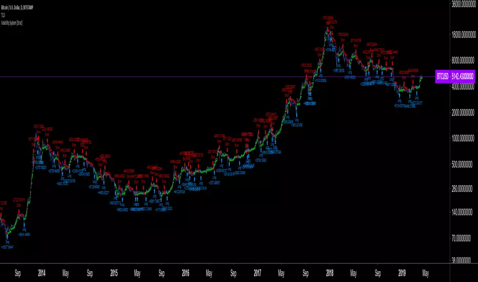
Multi-timeframe 24 moving averages + BB+SAR+Supertrend+VWAP █ OVERVIEW
The script allows to display up to 24 moving averages ("MA"'s) across 5 timeframes plus two bands (Bollinger Bands or Supertrend or Parabolic SAR or VWAP bands) each from its own timeframe.
The main difference of this script from many similar ones is the flexibility of its settings:
- Bulk enable/disable and/or change properties of several MAs at once.
- Save 3 of your frequently used templates as presets using CSV text configurations.
█ HOW TO USE
Some use examples:
In order to "show 31, 50, 200 EMAs and 20, 100, 200 SMAs for each of 1H, 4H, D, W, M timeframes using blue for short MA, yellow for mid MA and red for long MA" use the settings as shown on a screenshot below.
In order to "Show a band of chart timeframe MA's of lengths 5, 8, 13, 21, 34, 55, 100 and 200 plus some 1H, 4H, D and W MAs. Be able to quickly switch off the band of chart tf's MAs. For chart timeframe MA's only show labels for 21, 100 and 200 EMAs". You can set TF1 and TF2 to chart's TF and set you fib MAs there and configure fixed higher timeframe MAs using TF3, TF4 and TF5 (e.g. using 1H, D and W timeframes and using 1H 800 in place of 4H 200 MA). However, quicker way may be using CSV - the syntax is very simple and intuitive, see Preset 2 as it comes in the script. You can easily switch chart tf's band of MAs by toggling on/off your chart timeframe TF's (in our example, TF1 and TF2).
The settings are either obvious or explained in tooltips.
Note 1: When using group settings and CSV presets do not forget that individual setting affected will no have any effect. So, if some setting does not work, check whether it is overridden with some group setting or a CSV preset.
Note 2: Sometimes you can notice parts of MA's hanging in the air, not lasting up to the last bar. This is not a bug as explained on this screenshot:
█ FOR DEVELOPERS
The script is a use case of my CSVParser library, which in turn uses Autotable library, both of which I hope will be quite helpful. Autotable is so powerful and comprehensive that you will hardly ever wish to use normal table functions again for complex tables.
The indicator was inspired by Pablo Limonetti's url=https://www.tradingview.com/script/nFs56VUZ/]Multi Timeframe Moving Averages and Raging @RagingRocketBull's # Multi SMA EMA WMA HMA BB (5x8 MAs Bollinger Bands) MAX MTF - RRB
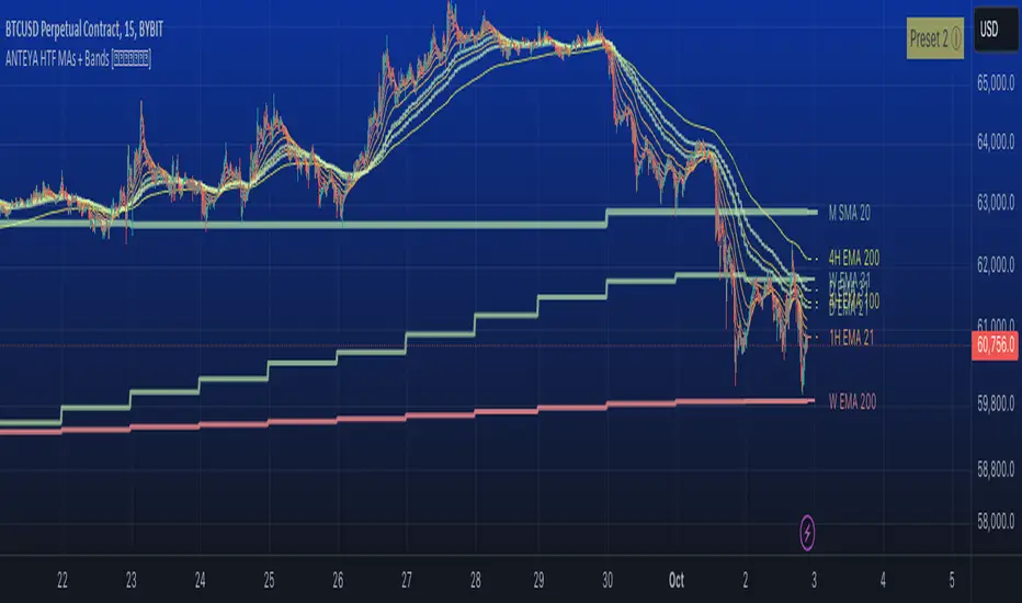
Vorse4**Vorse4 Indicator**
The Vorse4 Indicator is a technical analysis tool that combines Chaikin Oscillator, Intraday Momentum Index (IMI), MACD, and Parabolic SAR indicators. This indicator generates trading signals when all four indicators simultaneously provide buy or sell signals and visually presents these signals on the chart.
**How to Use:**
1. Buy signal: A buy signal is generated when there is a positive crossover in the Chaikin Oscillator, the IMI is above 50, the MACD line crosses the signal line upwards, and the price is above the Parabolic SAR. It is marked with a green arrow below the chart.
2. Sell signal: A sell signal is generated when there is a negative crossover in the Chaikin Oscillator, the IMI is below 50, the MACD line crosses the signal line downwards, and the price is below the Parabolic SAR. It is marked with a red arrow above the chart.
3. Turning zones: Areas with a high probability of transitioning from buy to sell or sell to buy are marked in yellow. These zones are determined by monitoring turning points in the Chaikin Oscillator, MACD, and Intraday Momentum Index.
**How to Apply:**
1. In your TradingView chart, go to the indicators menu and search for the "Vorse4" indicator.
2. Add the indicator to your chart. You will see green and red arrows indicating buy and sell signals, as well as yellow-colored areas representing turning zones on your chart.
3. Observe the buy and sell signals and trade according to your strategy. Analyze the performance of the indicator on historical data to evaluate the reliability of the signals.
**Note:** You can adjust the indicator parameters to balance the frequency and accuracy of buy and sell signals. Each strategy has a different risk-reward balance, so you can try different values to find the one that works best for you.
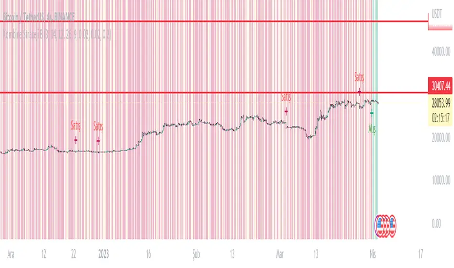
The Witcher [30MIN] - AlertsHello,
This is the Witcher Bot
This bot is got best performance at BTCUSDTPERP BINANCE FUTURES
this is bot for leverage 1x,
I tried focusing at highest % profitable trades, bot could be optimalised to even higher profit net.
TP: 1.1
SL: 8.2
Stop-loss unfortunelly have to be high to avoid bear/bull traps
The core of this strategy is trend strenght ( MONEY FLOW INDKES)
Strategy can only open position on strong price movment, to avoid wrong decision
Settings are set for highest profitable trades %
Bot using 10 indicators to trigger basic condtition for long and short :
1) ADX - Is one of the most powerful and accurate trend indicators. ADX measures how strong a trend is, and can give valuable information on whether there is a potential trading opportunity.
2) RSI - value helps strategy to stop trade in right time. When RSI is overbought strategy don't open new longs , also when RSI is oversold strategy don't open new shorts
3) TREND STRENGHT
4) JURIK MOVING AVERAGE - The Jurik Moving Average indicator is one of the surest ways to smoothen price curves within a minimum time lag. The indicator offers currency traders one of the best price filters during strong price moves. In this time, when bitcoin price action is so strong, this indicator is necessary.
5) SAR - The parabolic SAR is a technical indicator used to determine the price direction of an asset, as well as draw attention to when the price direction is changing. SAR supporting bot, to not open new trades when the trends are slowly changing
6) TREND INDICATOR
7) MOMENTUM - Indicator istechnical analysis tool used to determine the strength or weakness of a stock's price. Momentum measures the rate of the rise or fall of stock prices. Common momentum indicators include the relative strength index ( RSI ) and moving average convergence divergence ( MACD ).
8) OBV - On-balance volume (OBV) is a technical trading momentum indicator that uses volume flow to predict changes in stock price.
9) FAST MA - like previous ones this is for better view of trends, and correctly define the trends, also Speed_MA are using for predict the future price action.
10) RANGE FILTER - this indicator is for the better view of trends, define trends, that is important for every bull/bear traps which helps a lot becouse of the very variable trends.
I decided to add momentum indicator to strategy, to make a fast-reacting decision on lower timeframes at extremly price volatility
Also bot got additional EMA scalping option, which increase profit net but, in some situation, that could be risky.
For max security I recommend to turn off this option.
Commision are set at standard binancefutures VIP-0 = 0.04%
After converting strategy into study version, bot is ready for automation.
All the ploting color depends of adx value.
Strategy are not Repainting
For the source code I tried to keep as clean as I could
Enjoy

Cradle zone with BBand & SARHi All,
I have combined a number of indicators all into this 1 option.
It has the following:
> The Cradle zone represents a methodology to using the 10 and 20 EMA's at your selected time-frame.
Where the shading between the 10 and 20 EMA is green for an uptrend and red for a downtrend.
Default EMAs
10, 12, 20, and 50
> Those who are familiar using the Cradle method will find this option convenient.
> I have also added the Bollinger Band and Parabolic SAR as additional options to this item, to help give additional information by default.
Good luck with your trading strategy.
Please don't forget to give me a tick\like, as I would appreciate it.
Regards,
S.Sari /CryptoProspa

SMA/pivot/Bollinger/MACD/RSI en pantalla gráficoMulti-indicador con los indicadores que empleo más pero sin añadir ventanas abajo.
Contiene:
Cruce de 3 medias móviles
La idea es no tenerlas en pantalla, pero están dibujadas también. Yo las dejo ocultas salvo que las quiera mirar para algo.
Lo que presento en pantalla es la media lenta con verde si el cruce de las 3 marca alcista, amarillo si no está claro y rojo si marca bajista.
Pivot
Normalmente los tengo ocultos pero los muestro cuando me interesa. Están todos aunque aparezcan 2 seguidos.
Bandas de Bollinger
No dibujo la línea central porque empleo la media como tal.
Parabollic SAR
Lo empleo para dibujar las ondas de Elliott como postula Matías Menéndez Larre en el capítulo 11 de su libro "Las ondas de Elliott". Así que, aunque se puede mostrar, lo mantengo oculto y lo que muestro es dónde cambia (SAR cambio).
MACD
No está dibujado porque necesitaría sacarlo del gráfico.
Marco en la parte superior cuándo la señal sobrepasa al MACD hacia arriba o hacia abajo con un flecha indicando el sentido de esta señal.
RSI
Similar al MACD pero en la parte inferior.
Probablemente, programe otro indicador para visualizar en una ventanita MACD, RSI y volumen todo junto. El volumen en la principal hay veces que no te permite ver bien alguna sombra y los otros 2 te quitan mucho espacio para graficar si los tienes permanentemente en 2 ventanas separadas.
AVGO Advanced Day Trading Strategy📈 Overview
The AVGO Advanced Day Trading Strategy is a comprehensive, multi-timeframe trading system designed for active day traders seeking consistent performance with robust risk management. Originally optimized for AVGO (Broadcom), this strategy adapts well to other liquid stocks and can be customized for various trading styles.
🎯 Key Features
Multiple Entry Methods
EMA Crossover: Classic trend-following signals using fast (9) and medium (16) EMAs
MACD + RSI Confluence: Momentum-based entries combining MACD crossovers with RSI positioning
Price Momentum: Consecutive price action patterns with EMA and RSI confirmation
Hybrid System: Advanced multi-trigger approach combining all methodologies
Advanced Technical Arsenal
When enabled, the strategy analyzes 8+ additional indicators for confluence:
Volume Price Trend (VPT): Measures volume-weighted price momentum
On-Balance Volume (OBV): Tracks cumulative volume flow
Accumulation/Distribution Line: Identifies institutional money flow
Williams %R: Momentum oscillator for entry timing
Rate of Change Suite: Multi-timeframe momentum analysis (5, 14, 18 periods)
Commodity Channel Index (CCI): Cyclical turning points
Average Directional Index (ADX): Trend strength measurement
Parabolic SAR: Dynamic support/resistance levels
🛡️ Risk Management System
Position Sizing
Risk-based position sizing (default 1% per trade)
Maximum position limits (default 25% of equity)
Daily loss limits with automatic position closure
Multiple Profit Targets
Target 1: 1.5% gain (50% position exit)
Target 2: 2.5% gain (30% position exit)
Target 3: 3.6% gain (20% position exit)
Configurable exit percentages and target levels
Stop Loss Protection
ATR-based or percentage-based stop losses
Optional trailing stops
Dynamic stop adjustment based on market volatility
📊 Technical Specifications
Primary Indicators
EMAs: 9 (Fast), 16 (Medium), 50 (Long)
VWAP: Volume-weighted average price filter
RSI: 6-period momentum oscillator
MACD: 8/13/5 configuration for faster signals
Volume Confirmation
Volume filter requiring 1.6x average volume
19-period volume moving average baseline
Optional volume confirmation bypass
Market Structure Analysis
Bollinger Bands (20-period, 2.0 multiplier)
Squeeze detection for breakout opportunities
Fractal and pivot point analysis
⏰ Trading Hours & Filters
Time Management
Configurable trading hours (default: 9:30 AM - 3:30 PM EST)
Weekend and holiday filtering
Session-based trade management
Market Condition Filters
Trend alignment requirements
VWAP positioning filters
Volatility-based entry conditions
📱 Visual Features
Information Dashboard
Real-time display of:
Current entry method and signals
Bullish/bearish signal counts
RSI and MACD status
Trend direction and strength
Position status and P&L
Volume and time filter status
Chart Visualization
EMA plots with customizable colors
Entry signal markers
Target and stop level lines
Background color coding for trends
Optional Bollinger Bands and SAR display
🔔 Alert System
Entry Alerts
Customizable alerts for long and short entries
Method-specific alert messages
Signal confluence notifications
Advanced Alerts
Strong confluence threshold alerts
Custom alert messages with signal counts
Risk management alerts
⚙️ Customization Options
Strategy Parameters
Enable/disable long or short trades
Adjustable risk parameters
Multiple entry method selection
Advanced indicator on/off toggle
Visual Customization
Color schemes for all indicators
Dashboard position and size options
Show/hide various chart elements
Background color preferences
📋 Default Settings
Initial Capital: $100,000
Commission: 0.1%
Default Position Size: 10% of equity
Risk Per Trade: 1.0%
RSI Length: 6 periods
MACD: 8/13/5 configuration
Stop Loss: 1.1% or ATR-based
🎯 Best Use Cases
Day Trading: Designed for intraday opportunities
Swing Trading: Adaptable for longer-term positions
Momentum Trading: Excellent for trending markets
Risk-Conscious Trading: Built-in risk management protocols
⚠️ Important Notes
Paper Trading Recommended: Test thoroughly before live trading
Market Conditions: Performance varies with market volatility
Customization: Adjust parameters based on your risk tolerance
Educational Purpose: Use as a learning tool and customize for your needs
🏆 Performance Features
Detailed performance metrics
Trade-by-trade analysis capability
Customizable risk/reward ratios
Comprehensive backtesting support
This strategy is for educational purposes. Past performance does not guarantee future results. Always practice proper risk management and consider your financial situation before trading.
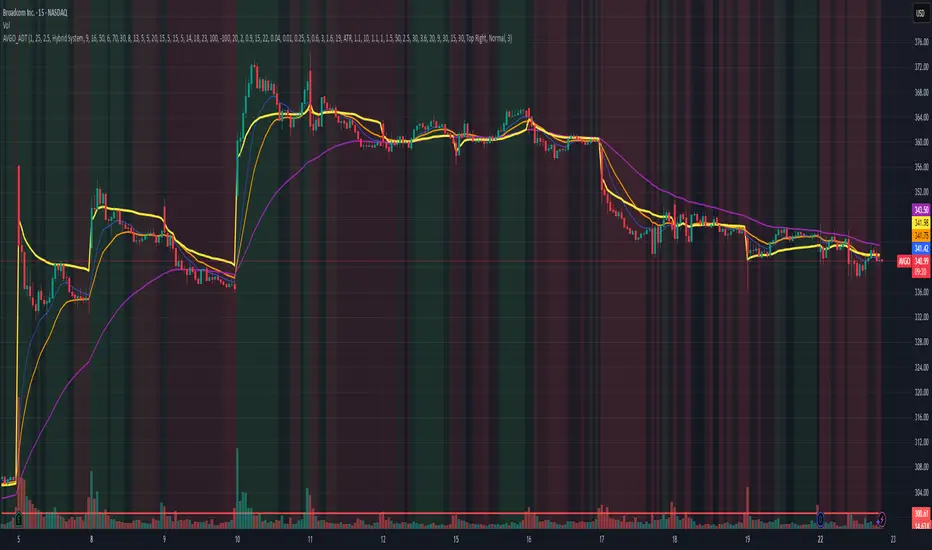
Dubic EMA StrategyThe Dubic EMA Strategy is a trend-following and volatility-aware strategy that combines dual EMA filters with intelligent range and noise detection to provide clean, actionable entries. It's designed to avoid choppy markets, enhance trade precision, and adapt to different market conditions.
✅ Key Features:
Dual EMA Filter: Enters long when price is above both EMA High & EMA Low, and short when below both.
Range Filter: Avoids entries during tight consolidations or sideways markets.
Volatility Filter: Prevents trading in low-ATR conditions.
Dynamic Risk Management:
ATR-based or fixed % Stop Loss and Take Profit.
Optional Parabolic SAR trailing stop.
One Trade per Trend: Prevents re-entry until trend direction changes.
Unbroken Range Visualization: Detects and displays consolidation zones that can lead to breakouts.
Alerts & Labels: Clean BUY/SELL signals with alerts and chart labels.
🧩 Customization Options:
Adjustable EMA length
Toggle between ATR or % based SL/TP
Volatility threshold
Range detection sensitivity
Enable/disable SAR trailing stop
This strategy works best on trending assets and timeframes with volatility (e.g., crypto, forex, indices). Suitable for both manual trading and automation.
🛠️ Built for clarity, control, and precision.
📈 Backtest, optimize, and deploy with confidence.
