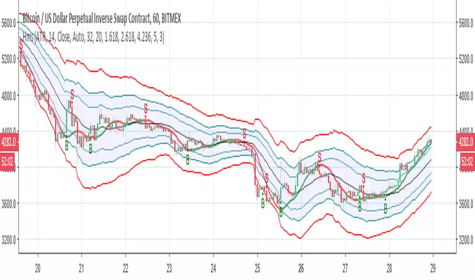
Hull modelius take profit and stop lossThis model has Hull moving average, fibs in form of Bollinger ,SMA and Modelius model with ATR for buy and sell power based on weis volume. Inside alerts for buy and sell. take profit and stop loss for both longs and shorts
so have fun
Cerca negli script per "profit"
Doji strategyThis is a simple strategy based on Doji star candlestick.
It places two orders: buy stop at doji star high or previous candle high and sell stop at doji star low or previous candle low.
Exit rules are with take profit and fixed stop loss or take profit and stop loss at doji min or max.
This strategy works very well with high time frames like Daily and Weekly because those are without noise in doji formation.
Each currency pair has its own optimal setting for TP and SL: it's up to user find the best ones.
I could implement SL based on ATR, maybe in next revision.
Please use comment section for any feedback.
Next improvement (only to whom is interested to this script and follows me): study with alerts on multiple tickers all at one. Leave a comment if you want to have access to study.

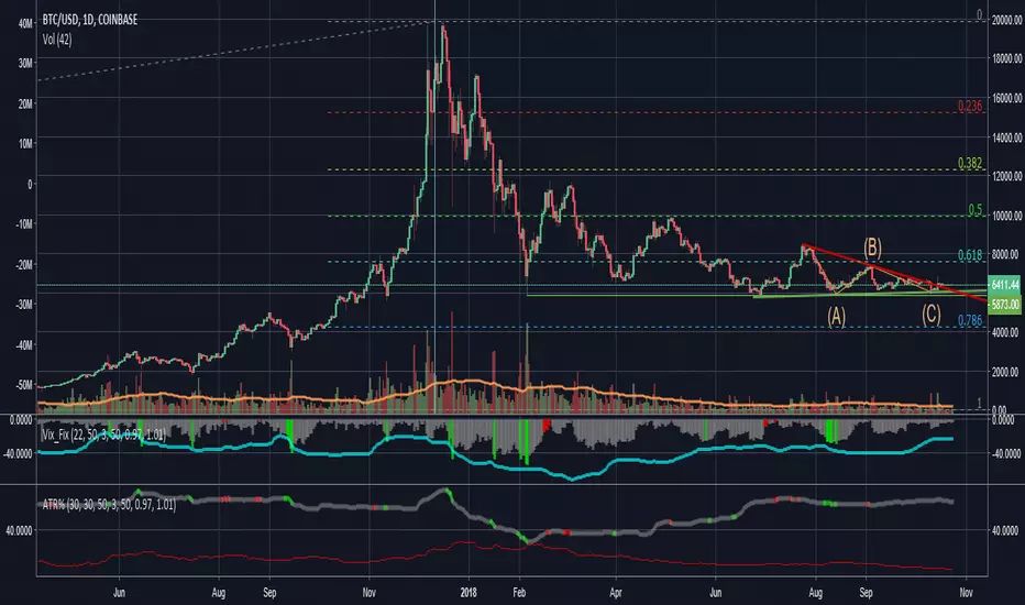
ATR and VIX For Profit Target and RSI LimitThe red line, based on ATR, should be used as a percentage gain goal. So I will set my profit targets based on this percentage.
The grey line is based on William's VIX and I use it to judge what RSI I should sell at.
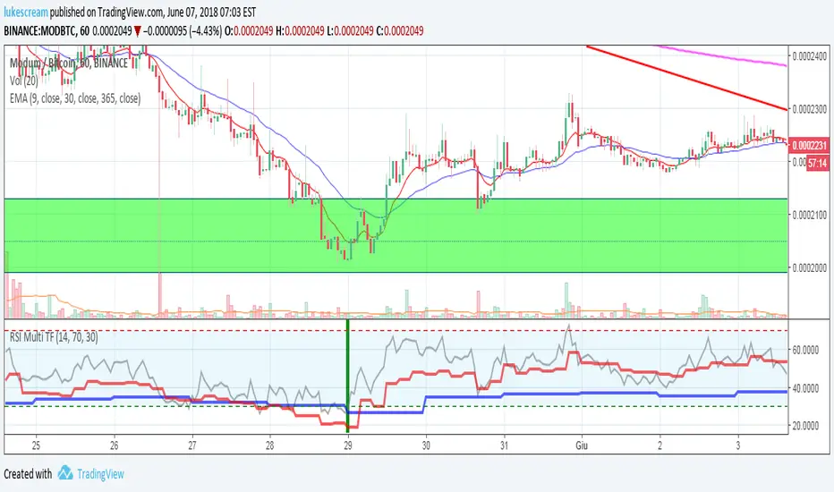
RSI Multi Time Frame - Spot Panic Sell Moments and profit!Union of three RSI indicators: 1h, 4h and daily. In order to show 1h RSI, you have to set it as active time frame on the chart.
Purpose: spot "triple oversold" moments, where all the three RSI are under the threshold, which is 30 by default but editable.
Target Market: Cryptocurrencies. Didn't try it on other ones, may work as well. Fits Crypto well as, by experience, I can tell it usually doesn't stay oversold for long.
When the market panics and triple oversold occurs, the spot is highlighted by a green vertical bar on the indicator.
The indicator highlights triple overbought conditions as well (usually indicating strong FOMO), but I usually don't use it as a signal.
I suggest to edit the oversold threshold in order to make it fit the coin you're studying, minimizing false positives.
Special thanks to Heavy91, a Discord user, for inspiring me in this indicator.
Any editing proposal is welcome!
I reposted this script, as the first time I wrote it in Italian. Sorry for that.

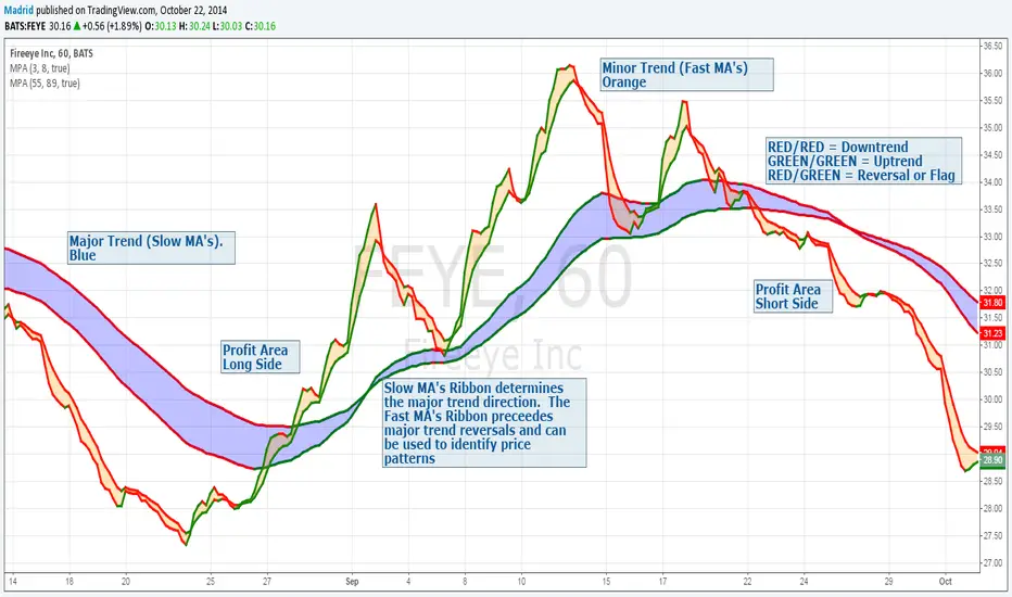
Madrid Profit AreaThis study displays a ribbon made of two moving averages identified by a filled Area. This provides visual aids to determine the trend direction and pivot points. The moving average will be Red if its value is decreasing, and green if it is increasing. When both MA's are the same color we have a trend direction. If those are different then we have a trend reversal and a pivot point.
If combined with another ribbon then it can be configured so we have a pair of slow MA's and another pair of fast MA's , this can visually determine if the price is in bull or bear territory following the basic rules:
1. Fast MA pair above the slow MA Pair = Bullish
2. Fast MA pair below the slow MA Pair = Bearish
3. If the fast MA crosses over the slow MA it is a Bullish reversal
4. If the fast MA crosses below the the slow MA, it is a Bearish reversal.
The use of the ribbons without the price bars or line reduces the noise inherent to the price
Opening Range Breakout with 2 Profit Targets.Opening Range Breakout with 2 Profit Targets.
Updated Indicator now works on all Symbols with Many Different Session Options.
***Known PineScript Issue…While the Opening Range is being Formed the lines only adjust for that individual bar. Just reset Indicator after Opening Range Completes.
***All Times are Based on New York Time
Session Options Forex U.S. Banks Open (8:00), Gold U.S. Open (8:20), Oil U.S. Open (9:00), U.S. Cash Session - Stocks (9:30), NY Forex Open (17:00) , Europe Open (02:00), or if you choose Setting 0 the Session Runs from 00:00 to 00:00 (Midnight to Midnight).
***Ability to use 60 minute Opening Range, 30 minute, 15 minute, and many other options.
***However you can manually change the times in the Inputs Tab to adjust for any session you prefer. This is useful for Day Light Savings Adjustments. Also the default times work if your charts are set to EST Time. If you use A different time zone in your settings you need to Adjust the times in the inputs tab.
Initially Opening Range High and Low plot as Yellow Lines. If Price Goes Above Opening Range then Line Turns Green. If Price Goes Below Opening Range Line Turns Red.
By default the First Profit Target is 1/2 the Width of the Opening Range and the 2nd Profit Target is 1 Times the Opening Range. However these are Adjustable in the Inputs Tab.
By Default the Opening Range Length is 1 Hour. However, you can Change the Opening Range Length to 15 min, 30 min, 2 hours etc. in the Inputs Tab.
Plots a 1 Above or Below Candle when 1st Profit Target is Achieved, and a 2 when 2nd Profit Target is Achieved.

ES/NQ Price Action Sync See when ES & NQ move in syncSee when ES & NQ move in sync — revealing real market momentum at a glance.”
⚖️ ES/NQ Price Action Sync
Discover when the market moves as one.
This indicator tracks when S&P 500 Futures (ES1!) and Nasdaq Futures (NQ1!) align in momentum — helping you spot broad-market confirmation or early divergence in real time.
🧠 Concept
The ES/NQ relationship often reveals the market’s underlying strength or hesitation. When both indices turn bullish or bearish together with meaningful movement, that’s a sign of true market alignment.
When they disagree — expect mixed momentum and possible reversals.
⚙️ Features
✅ Highlights new bullish and bearish syncs on chart
✅ Dynamic info table showing % change and direction for each index
✅ Optional triangle markers for clean visual cues
✅ Alert conditions for new sync events
✅ Adjustable lookback and minimum-move filters
💡 How to Use
Use this as a market-context tool, not a direct buy/sell signal.
When both indices sync, intraday trends often hold better; when they diverge, momentum may fade.
Combine it with your own system or higher-time-frame analysis for confirmation.
📊 Why Traders Love It
Simple idea — powerful insight.
This tool helps traders instantly see when “the market machine” is running in harmony… or pulling in opposite directions.
⚠️ Disclaimer:
This script is for educational and analytical purposes only.
It does not provide financial advice or trading signals. Always perform your own research before making trading decisions.

DIP BUYING by HAZEREAL BUY THE DIP - Educational Price Movement Indicator
This technical indicator is designed for educational purposes to help traders identify potential price reversal opportunities in equity markets, particularly focusing on NASDAQ-100 index tracking instruments and technology sector ETFs.
Key Features:
Monitors price movements relative to recent highs over customizable lookback periods
Identifies two distinct price decline thresholds: standard (5%+) and extreme (12.3%+)
Visual signals with triangular markers and background color zones
Real-time data table showing current metrics and status
Customizable alert system with webhook-ready JSON formatting
Clean overlay design that doesn't obstruct price action
How It Works:
The indicator tracks the highest price within a specified lookback period and calculates the percentage decline from that high. When price drops below the minimum threshold, it generates visual buy signals. The extreme threshold triggers enhanced alerts for more significant market movements.
Best Use Cases:
Educational analysis of market volatility patterns
Identifying potential support levels during market corrections
Studying historical price behavior around significant declines
Risk management and position sizing education
Important Note: This is a technical analysis tool for educational purposes only. All trading decisions should be based on comprehensive analysis and appropriate risk management. Past performance does not guarantee future results.

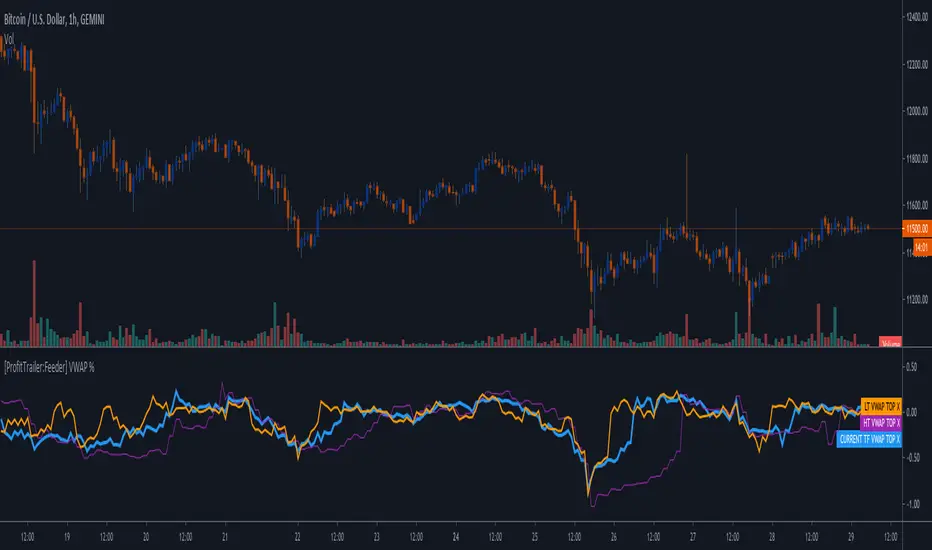
[ProfitTrailer:Feeder] VWAP %This script will help you create a strategy bases on VWAP % on BaseCoin & Top xx coin settings.
Enjoy & Like and follow if you like this kind of content.
[ProfitTrailer:Feeder] Market Trends Top X / BTCThis script will help you determine your MarketConditions Grouping for PtFeeder. You're able to input the specific top 10/20/xx pairs you want to use to fine-tune your groupings as well as specific BasePairs, there values will be automatically printed on the chart!
When measuring top coins trend, this is how many top coins to check by volume from the exchanges that you have configured PT Feeder for. For, the top 50 coins will be checked and their price change over the MeasureTimes property and the average change calculated. This average is used for the MaxTopCoinAverageChange property
If you like this kind of content, please 'like' and 'follow' and I'll continue publishing these kind of scripts!
Enjoy!

Profitable L 1800 Candle Highlight [Beta]
Certainly! Here's a user guide for the provided Pine Script code:
User Guide: 1800 Candle Highlight Indicator
Overview:
The "1800 Candle Highlight" indicator is designed to visually emphasize the 18:00 (6:00 PM) candle on the chart, providing clarity on its open and close prices, and highlighting its timeframe with a distinctive color.
Key Features:
Candle Highlighting: The indicator identifies the candle that opens at 18:00 and visually distinguishes it from other candles on the chart.
Open and Close Prices: The indicator plots the open and close prices of the 18:00 candle as step lines, making it easy to identify price movements during that timeframe.
Background Color: It colors the background within the 18:00 candle's timeframe with a transparent blue shade, providing further emphasis on that period.
Start Marker: A downward triangle shape marks the start of the 18:00 candle, aiding in identifying the beginning of the highlighted timeframe.
Usage:
Overlay: The indicator is designed to be overlaid on the price chart, allowing users to visualize the highlighted candle alongside price movements.
Interpretation: Traders can observe the open and close prices of the 18:00 candle relative to previous and subsequent candles, aiding in analysis and decision-making.
Timeframe Focus: The highlighted candle's timeframe can serve as a reference point for analyzing price action during specific hours, such as the end of a trading day.
Installation:
Access: Users can access the Pine Script editor within the TradingView platform to create a new indicator.
Copy and Paste: Copy the provided Pine Script code and paste it into the editor.
Save and Apply: Save the indicator and apply it to the desired chart, adjusting settings as needed.
Customization:
Color Scheme: Users can customize the colors used for highlighting, open/close prices, and background to suit their preferences and chart aesthetics.
Styling: Adjustments can be made to line styles, widths, and marker sizes to enhance visibility and clarity.
Compatibility:
The indicator is compatible with TradingView's Pine Script version 5 and can be applied to various financial instruments and timeframes supported by the platform.
Disclaimer:
The "1800 Candle Highlight" indicator is provided for informational purposes only and should not be considered as financial advice. Users are encouraged to conduct thorough analysis and consider multiple factors before making trading decisions.

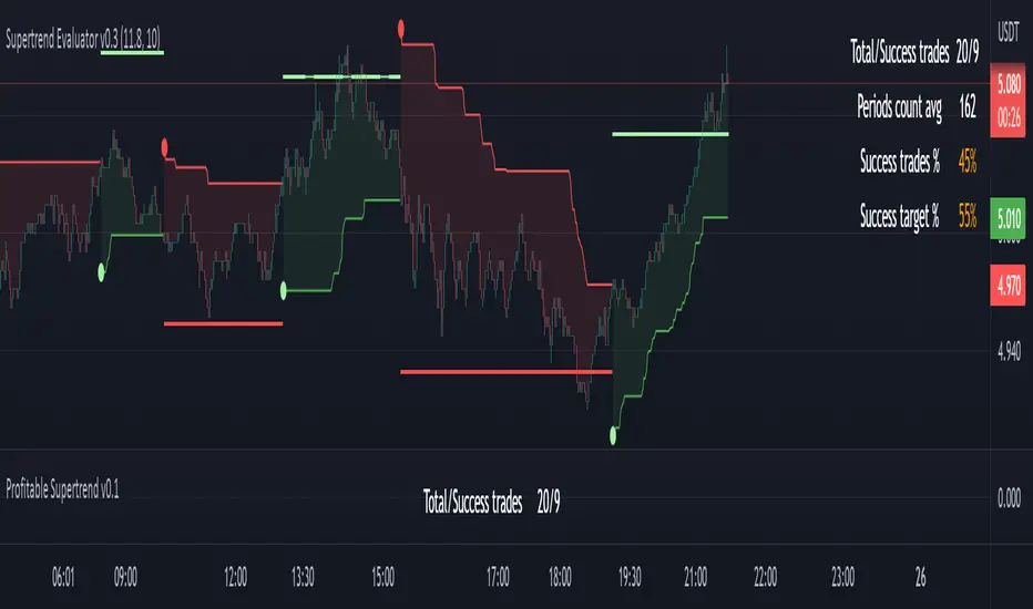
Profitable Supertrend v0.1 - AlphaThis a script to try detect the best combination of supertrend parameters in a space of time. Sadly the script is slow. Evaluate all possibilities params is hard for a pinescript and my knowledge too. In some cases, when you want evaluate many time could be the script fails for timeout. Perhaps with time I could enhance. For this problem of speed the calculate of combinatios it's not complete: In factor use a increment of 0.2 in each param (0.1, 0.3, 0.5 ...) in period the increment for each value is 3. The range for factor it's from 3.0 to 12.0. The range of period it's from 10 to 43
My knowledge don't let me go more far. Perhaps with time I can enhance the script.
PMax on RSI with Tillson T3Profit Maximizer Indicator on RSI with Tillson T3 Moving Average:
PMax uses ATR calculation inside, for this reason users couldn't manage to use PMax on RSI because RSI indicator doesn't have High and Low values in bars, but ATR needs that values. So I personally calculate RSI in a different way to have High and Low values of RSI wrt price bars.
IMPORTANT:
Because of the sudden movements and divergences on RSI, this indicator must firstly optimized for the charts before using. Optimization can be held by users for the meaningful parameters for each chart.
3 parameters are critical when optimizing:
First: Multiplier
Second: Tillson T3 Length
Third: T3 Volume Factor
Here are some information about Profit Maximizer:
PMax Indicator:
PMax Screener and Strategy:

PMax Explorer STRATEGY & SCREENERProfit Maximizer - PMax Explorer STRATEGY & SCREENER screens the BUY and SELL signals (trend reversals) for 20 user defined different tickers in Tradingview charts.
Simply input the name of the ticker in Tradingview that you want to screen.
Terminology explanation:
Confirmed Reversal: PMax reversal that happened in the last bar and cannot be repainted.
Potential Reversal: PMax reversal that might happen in the current bar but can also not happen depending upon the timeframe closing price.
Downtrend: Tickers that are currently in the sell zone
Uptrend: Tickers that are currently in the buy zone
Screener has also got a built in PMax indicator which users can confirm the reversals on graphs.
Screener explores the 20 tickers in current graph's time frame and also in desired parameters of the SuperTrend indicator.
Also you can optimize the parameters manually with the built in STRATEGY version.
PMax indicator :
Profit Maximizer - PMax is a brand new indicator developed by me.
It's a combination of two trailing stop loss indicators;
One is Anıl Özekşi's MOST (Moving Stop Loss) Indicator
and the other one is well known ATR based SuperTrend
Profit Maximizer - PMax tries to solve this problem. PMax combines the powerful sides of MOST (Moving Average Trend Changer) and SuperTrend (ATR price detection) in one indicator.
Backtest and optimization results of PMax are far better when compared to its ancestors MOST and SuperTrend. It reduces the number of false signals in sideways and give more reliable trade signals.
PMax is easy to determine the trend and can be used in any type of markets and instruments. It does not repaint.
The first parameter in the PMax indicator set by the three parameters is the period/length of ATR.
The second Parameter is the Multiplier of ATR which would be useful to set the value of distance from the built in Moving Average.
I personally think the most important parameter is the Moving Average Length and type.
PMax will be much sensitive to trend movements if Moving Average Length is smaller. And vice versa, will be less sensitive when it is longer.
As the period increases it will become less sensitive to little trends and price actions.
In this way, your choice of period, will be closely related to which of the sort of trends you are interested in.
We are under the effect of the uptrend in cases where the Moving Average is above PMax;
conversely under the influence of a downward trend, when the Moving Average is below PMax.
Built in Moving Average type defaultly set as EMA but users can choose from 8 different Moving Average types like:
SMA : Simple Moving Average
EMA : Exponential Movin Average
WMA : Weighted Moving Average
TMA : Triangular Moving Average
VAR : Variable Index Dynamic Moving Average aka VIDYA
WWMA : Welles Wilder's Moving Average
ZLEMA : Zero Lag Exponential Moving Average
TSF : True Strength Force
Tip: In sideways VAR would be a good choice
You can use PMax default alarms and Buy Sell signals like:
1-
BUY when Moving Average crosses above PMax
SELL when Moving Average crosses under PMax
2-
BUY when prices jumps over PMax line.
SELL when prices go under PMax line.

McGinley Dynamic debugged🔍 McGinley Dynamic Debugged (Adaptive Moving Average)
This indicator plots the McGinley Dynamic, a mathematically adaptive moving average designed to reduce lag and better track price action during both trends and consolidations.
✅ Key Features:
Adaptive smoothing: The McGinley Dynamic adjusts itself based on the speed of price changes.
Lag reduction: Compared to traditional moving averages like EMA or SMA, McGinley provides smoother yet responsive tracking.
Stability fix: This version includes a robust fix for rare recursive calculation issues, particularly on low-priced historical assets (e.g., Wipro pre-2000).
⚙️ What’s Different in This Debugged Version?
Implements manual clamping on the source / previous value ratio to prevent mathematical spikes that could cause flattening or distortion in the plotted line.
Ensures more stable behavior across all instruments and timeframes, especially those with historically low price points or volatile early data.
💡 Use Case:
Ideal for:
Trend confirmation
Entry filtering
Adaptive support/resistance visualization
Improving signal precision in low-volatility or high-noise environments
⚠️ Notes:
Works best when combined with volume filters or other trend indicators for validation.
This version is optimized for visual use—for signal generation, consider pairing it with additional logic or thresholds.

PROFIT INDICATORFirst let me tell you which indicators have been used in this script so that you have the confidence while taking the trade:
(a) Bollinger Band with 20 SMA Inside it - Currently it is off, you can turn it on from settings.
(b) HMA 33, I have added the option of using two HMA's simultaneously. You can use HMA, EMA, SMA as per your settings and it would be color trending.
(c) VWAP- you can turn it on from settings
(d) CPR- you can turn it on from settings
(e) EMA's 20, 50, 200. Currently off, you can turn it on from settings.
(d) SMA's 50 and 200. Currently off, yu can turn it on from settings, if you want to use 20 SMA you can use bollinger band basis that is 20 period SMA.
(f) Trend bar at bottom on the basis of 50 EMA.
(g) Half Trend
(h) Trend strength Detector
(d) EMA 50 high and low to show the pac channel. I am not using this however as per request I have added this. Currently, it is trun on and you can turn it off from settings.
(f) Auto Fib levels
Please use a stick note for few days and mention imp notes before taking trade to check if all the conditions are matching to take the trade.
Buy Condition:-
1. Bolling band should be widely open.
2. Check the support and resistance from CPR. Candle should close above support in green.
3. Check the trend bar at bottom, it should be green, if it is grey in colour dont enter in trade.
4. Candle should be closing above EMA 50 and its upto you if you need additional confirmation, you can use EMA 20, 50, 200 and SMA 50 and 200, this is optional.
5. You can use VWAP as support or resistance and you can turn it on from settings.
6. Trending HMA of 33 should be in green for buy.
7. Half trend Indicator should give buy signal.
8. Trend Strength Indicator for checking the strength of the trend, if the arrow is big upside, you can go for buy.
9. Exit from buy trade when it start showing very small arrow which means trend is about to change.
10.Exit buy trade at 61.8 Fib level
Sell Condition:-
1. Bolling band should be widely open.
2. Check the support and resistance from CPR. Candle should close below resistance in red.
3. Check the trend bar at bottom, it should be red, if it is grey in colour dont enter in trade.
4. Candle should be closing below EMA 50 and its upto you if you need additional confirmation, you can use EMA 20, 50, 200 and SMA 50 and 200, this is optional.
5. You can use VWAP as support or resistance and you can turn it on from settings.
6. Trending HMA of 33 should be in red for sell.
7. Half trend Indicator should give sell signal.
8. Trend Strength Indicator for checking the strength of the trend, if the arrow is big downside, you can go for sell.
9. Exit from sell trade when down arrows start showing very small in size which means trend is about to change.
10.Exit sell trade at 61.8 Fib level

PMax on Rsi w/T3 *Strategy*Profit Maximizer Indicator on RSI with Tillson T3 Moving Average:
PMax uses ATR calculation inside, for this reason users couldn't manage to use PMax on RSI because RSI indicator doesn't have High and Low values in bars, but ATR needs that values. So I personally calculate RSI in a different way to have High and Low values of RSI wrt price bars.
IMPORTANT:
Because of the sudden movements and divergences on RSI , this indicator must firstly optimized for the charts before using. Optimization can be held by users for the meaningful parameters for each chart.
3 parameters are critical when optimizing:
First: Multiplier
Second: Tillson T3 Length
Third: T3 Volume Factor
Says, Kıvanç Özbilgiç. Here's the strategy version for you to backtest & optimize properly.
Enjoy.

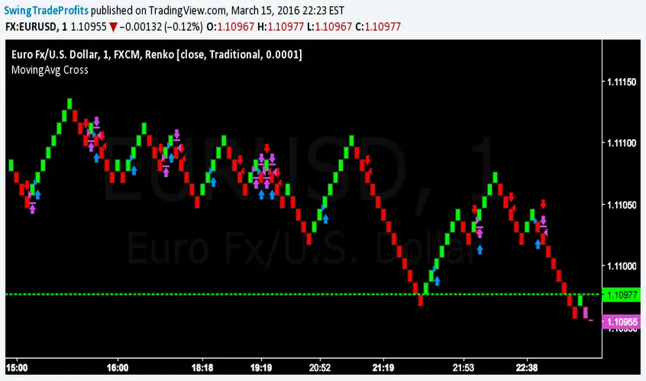
$EURUSD 1 Minute Chart StrategyYou must be using the renko chart with traditional settings with the block size set at .0001. This can be done by going to settings. Style at the bottom should be changed from ATR to traditional. The set the block size as .0001.
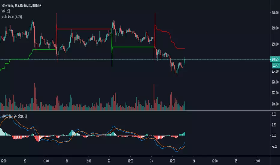
Profit target areaUpdate.
- you can specify count of bars used to detect reversal pattern
- you can specify count of bars used to determine lowest or highest price to place support or resistance
- area between lines is filled by green - ascending, red - descending trend
To trade:
- open position using stop command on S/R
- close position using limit command on retracement line
- close position when background colour indicates trend change
(erratum: last balloon on right should say "buy limit")

Retail Forex Sentiment Fear/Greed CurrencyPairsRetail Forex Sentiment Fear/Greed CurrencyPairs
Overview
The Retail Forex Sentiment Indicator provides sentiment data for major and cross currency pairs. This indicator displays retail trader positioning using retail brokers data, showing what percentage of retail traders are long or short on each forex pair.
Important: Indicator Split Notice
---------------------------------
Due to TradingView's limitation of 40 data requests per indicator, the original Retail Sentiment Indicator has been split into TWO separate indicators you will find on TradingView:
1. This indicator - Specialized for Forex currency pairs (30+ pairs)
[2. Retail Sentiment Indicator - Multi-Asset CFD & Fear/Greed Index - For indices, commodities, cryptocurrencies, and Fear/Greed indices
Please look at both indicators to access all available sentiment data.
Methodology and Scale Calculation
---------------------------------
This indicator operates on a **-50 to +50 scale** with zero representing perfect market equilibrium.
Scale Interpretation:
- **Zero (0)**: Market balance - exactly 50% of traders long, 50% short
- **Positive values**: Majority long (buying) pressure
- Example: If 63% of traders are long, the indicator shows +13 (63 - 50 = +13)
- **Negative values**: Majority short (selling) pressure
- Example: If 92% of traders are short, the indicator shows -42 (50 - 92 = -42)
Features
--------
- **Auto-Detection**: Automatically loads sentiment data based on the current chart symbol
- **Manual Selection**: Choose from 30+ supported currency pairs when auto-detection is unavailable
- **Visual Zones**: Clear greed/fear zones with color-coded backgrounds (green for fear zone, red for greed zone - contrarian colors)
- **Daily Updates**: Live sentiment data from retail CFD providers
Supported Currency Pairs
========================
Major Pairs
-----------
- EURUSD (most traded pair globally)
- GBPUSD (Cable)
USD Pairs
---------
- USDJPY, USDCHF, USDCAD
- USDPLN
PLN (Polish Zloty) Pairs
------------------------
- USDPLN, EURPLN, GBPPLN, CHFPLN
EUR Cross Pairs
---------------
- EURJPY, EURCHF, EURCAD, EURAUD, EURNZD, EURGBP
GBP Cross Pairs
---------------
- GBPJPY, GBPCHF, GBPCAD, GBPAUD, GBPNZD
AUD (Australian Dollar) Pairs
-----------------------------
- AUDUSD, AUDJPY, AUDCHF, AUDNZD, AUDCAD
NZD (New Zealand Dollar) Pairs
------------------------------
- NZDUSD, NZDJPY, NZDCHF, NZDCAD
CAD Cross Pairs
---------------
- CADJPY, CADCHF
CHF Cross Pairs
---------------
- CHFJPY
How to Use
----------
1. **Auto Mode** (Default): Enable "Auto-load Sentiment Data" checkbox to automatically display sentiment for the current chart's currency pair
2. **Manual Mode**: Disable auto-load and select from the dropdown menu for specific currency pairs
3. **Interpretation**:
- Values above 0 (green line) indicate retail traders are net long (greed/bullish sentiment)
- Values below 0 (red line) indicate retail traders are net short (fear/bearish sentiment)
- Extreme zones (+35 to +50 and -35 to -50) indicate strong positioning
Trading Strategy & Market Philosophy
====================================
Contrarian Trading Approach
---------------------------
The primary purpose of this indicator is based on the fundamental market principle that **the majority of retail forex traders are wrong most of the time**, and currency pairs typically move opposite to the positions held by the majority of retail participants.
Key Strategy Guidelines:
- **Contrarian Signal**: When the majority of retail traders are positioned on one side, consider opportunities in the opposite direction
- **Trend Exhaustion Signal**: When retail traders finally flip to trade WITH an established trend after being wrong for extended period, this often signals trend exhaustion
Interpretation Examples:
- High greed readings (majority long) -> Consider short opportunities
- High fear readings (majority short) -> Consider long opportunities
- Sudden sentiment flip during established trends -> Potential trend reversal signal
Forex-Specific Notes
====================
Currency Correlations
---------------------
When analyzing forex sentiment, consider that:
- USD pairs often move together (if retail is long EURUSD, they're often short USDJPY)
- Cross pairs can provide confirmation signals
- Comparing sentiment across related pairs can reveal broader positioning
Auto-Detection Support
----------------------
The indicator supports automatic detection of various broker ticker formats including:
- Standard pairs (EURUSD, GBPUSD, etc.)
- CME Futures symbols (6E, 6B, JY, etc.)
- Micro futures (M6E, M6B, MJY, etc.)
This functionality is powered by regex pattern matching. However, for some CME futures pairs—particularly those involving JPY, CAD, and CHF—auto-detection may not work properly. In such cases, disable the auto-load checkbox and manually select the ticker from the dropdown menu.
Technical Notes
---------------
- Built with PineScript v6
- Dynamic symbol detection with fallback options
- Optimized for performance with minimal resource usage
- Color-coded visualization with customizable zones
Data Sources
------------
This indicator uses curated sentiment data from retail CFD providers. Data is updated regularly and sourced from reputable financial data providers.
Data Infrastructure Status
--------------------------
Current Data Upload Process:
Please note that sentiment data uploads may occasionally experience minor interruptions. However, this should not pose significant issues as sentiment data typically changes gradually rather than rapidly.
Acknowledgments
---------------
We extend our gratitude to **TradingView** for enabling the use of custom data feeds based on GitHub repositories, making this comprehensive forex sentiment analysis possible.
Disclaimer
----------
This indicator is for educational and informational purposes only. Sentiment data should be used as part of a comprehensive trading strategy and not as the sole basis for trading decisions. Past performance does not guarantee future results. The contrarian approach described is a market theory and may not always produce profitable results. Forex trading involves significant risk of loss.
